The Lightweight Swin Transformer for Salinity Degree Classification in a Natural Saline Soil Environment

Abstract

Excessive salt in soil can significantly reduce crop yield and quality by hindering nutrient absorption. Accurate classification of soil salinization degree is very important for the development of effective management strategies. In this paper, we propose a novel deep learning-based method to identify the degree of soil salinization using a Swin Transformer model enhanced with token-based knowledge distillation. The Swin Transformer, as the backbone of the model, provides comprehensive contextual information and a larger receptive field, ensuring efficient feature extraction. By incorporating token-based distillation, we effectively reduce model size and inference time, overcoming the traditional challenges of large parameters in Transformer models. Our model achieves a classification accuracy of 96.3% on the saline soil datasets of three degrees categories, outperforming existing methods. Compared to the baseline model, the number of parameters is reduced by 80.8%, ensuring faster and more efficient salinity detection. This method not only enhances the accuracy of soil salinity classification but also offers a cost-effective solution, providing valuable data to guide agricultural practitioners in improving soil quality and optimizing land resource management.

1. Introduction

Saline soil usually occurs in arid or semi-arid regions [1]. Due to unreasonable irrigation systems, land degradation, and climate drought, a large amount of saline substances are accumulated in the soil [2]. Saline soils can damage the soil structure and prevent plants from absorbing water and nutrients, resulting in poor crop growth and reduced yields [3,4]. So, accurate identification of soil salinity is vital for intelligent field management and helps to provide decision support for the management and utilization of saline soils [5]. Current soil salinity monitoring primarily relies on manual electrical conductivity (EC) measurements and laboratory chemical analyses. Although the accuracy of these methods is high, the cost of equipment is high and depends on manpower, which makes it difficult to meet the large-scale dynamic monitoring needs of precision agriculture [6]. Consequently, developing automated, efficient, and accurate models for saline soil classification is essential. The integration of sensors and artificial intelligence (AI) into agriculture has significantly improved productivity, with machine learning (ML) and deep learning (DL) methods being widely adopted for soil classification and land use planning [7,8,9]. However, traditional ML methods struggle to capture high-level image features, have poor transferability, and are sensitive to outliers, leading to unstable results. DL methods, by contrast, offer better feature representation and robustness, making them suitable for automatic saline soil classification, although their application in this field is still limited.

DL has been extensively applied in agriculture, such as crop management [10], yield prediction [11], disease monitoring [12], weed detection [13,14], and water and land management [15]. Convolutional neural networks (CNNs) such as AlexNet, VGG16, ResNet50, and GoogLeNet have achieved high accuracy in crop-related tasks like corn and soybean leaf recognition [16,17]. To further improve classification accuracy, some studies employed image segmentation or feature enhancement techniques. For instance, Yan et al. used ETUnet to extract rice field features from UAV images and classify growth stages with 90% accuracy [18], while Hayıt et al. applied grayscale and color-scale depth features for CNN-based wheat disease classification [19]. Nevertheless, these methods are not end-to-end methods. Other studies enhanced performance through data augmentation and network fusion. Pual et al. combined VGG16 and VGG19 with data augmentation to classify tomato leaf diseases at 95% accuracy [20]. Kumar et al. used a bi-directional feature attention pyramid network for feature extraction to classify maize leaf diseases, achieving 94.87% classification accuracy [21]. C.K. et al. used a multilevel feature fusion network to extract image features. They combined it with ResNet50 and MFFN methods to classify tomato plant diseases with a maximum accuracy of 99.88% [22].

However, CNNs are inherently limited by local receptive fields, which constrain their ability to capture long-range spatial dependencies—an important requirement for soil salinity classification, given the spatial heterogeneity of saline areas and occlusion from vegetation such as Suaeda glauca. In this study, soil salinity was classified based on high-resolution RGB images taken by digital cameras. These images can directly and intuitively observe the key surface indicators of salinity, such as soil surface salt accumulation area and soil texture characteristics. In order to enable the model to effectively learn and identify salinity levels, the input image must have sufficient resolution and clarity to capture the subtle contrast between saline and non-saline areas. And the vision-based classification method requires the acquired image to minimize occlusion. Therefore, high-quality images are the basic prerequisite for the success of salinity classification methods.

Transformer models have shown excellent performance in these aspects and have been widely applied in various fields, such as remote sensing [23], industrial manufacturing [24], meteorology [25], medicine [26], and natural language processing [27]. Due to its outstanding performance, Transformer models can overcome these challenges in classifying salinity degrees by using the self-attention mechanism to capture long-distance dependencies. The Transformer model considers information from all input positions, regardless of the receptive field, which gives it an advantage in tasks that necessitate global information, such as salinity recognition. Moreover, in our task, the demand for inference time is higher. The computation of each position in the Transformer is independent and can be computed in parallel, which meets the requirement of efficient computation when processing data. Nonetheless, the Transformer model requires more computing resources than some lightweight models, resulting in a large amount of calculation and parameters.

In order to reduce the parameters while ensuring accuracy, this paper proposes a lightweight Swin Transformer–Knowledge Distillation (Swin-KD) model of soil salinity classification. In Swin-KD, the Swin Transformer model is used as the backbone to extract soil-rich characteristics. A knowledge distillation based on tokens is introduced into the backbone network to fully retain the ability to extract features and achieve the lightweight effect of the network. Therefore, we expect that this method will be feasible in accurately identifying different degrees of soil salinity. We hypothesize that a lightweight Transformer architecture enhanced with token-based knowledge distillation can achieve high-accuracy soil salinity classification while significantly reducing model complexity, making it suitable for real-time and large-scale agricultural monitoring. In summary, our contributions can be summarized as follows:

• We propose a lightweight Transformer model, Swin-KD, which integrates Swin Transformer with a token-based knowledge distillation framework to enhance classification accuracy while significantly reducing parameter count.
• A novel distillation strategy is introduced, where distillation tokens interact with class tokens via attention mechanisms, enabling effective knowledge transfer from the teacher model and improving both efficiency and performance.
• Experimental results on real-world saline soil datasets demonstrate that Swin-KD outperforms baseline models in both accuracy and inference speed, showing strong potential for practical applications in soil salinity monitoring.

2. Materials and Methods

2.1. Dataset Collection

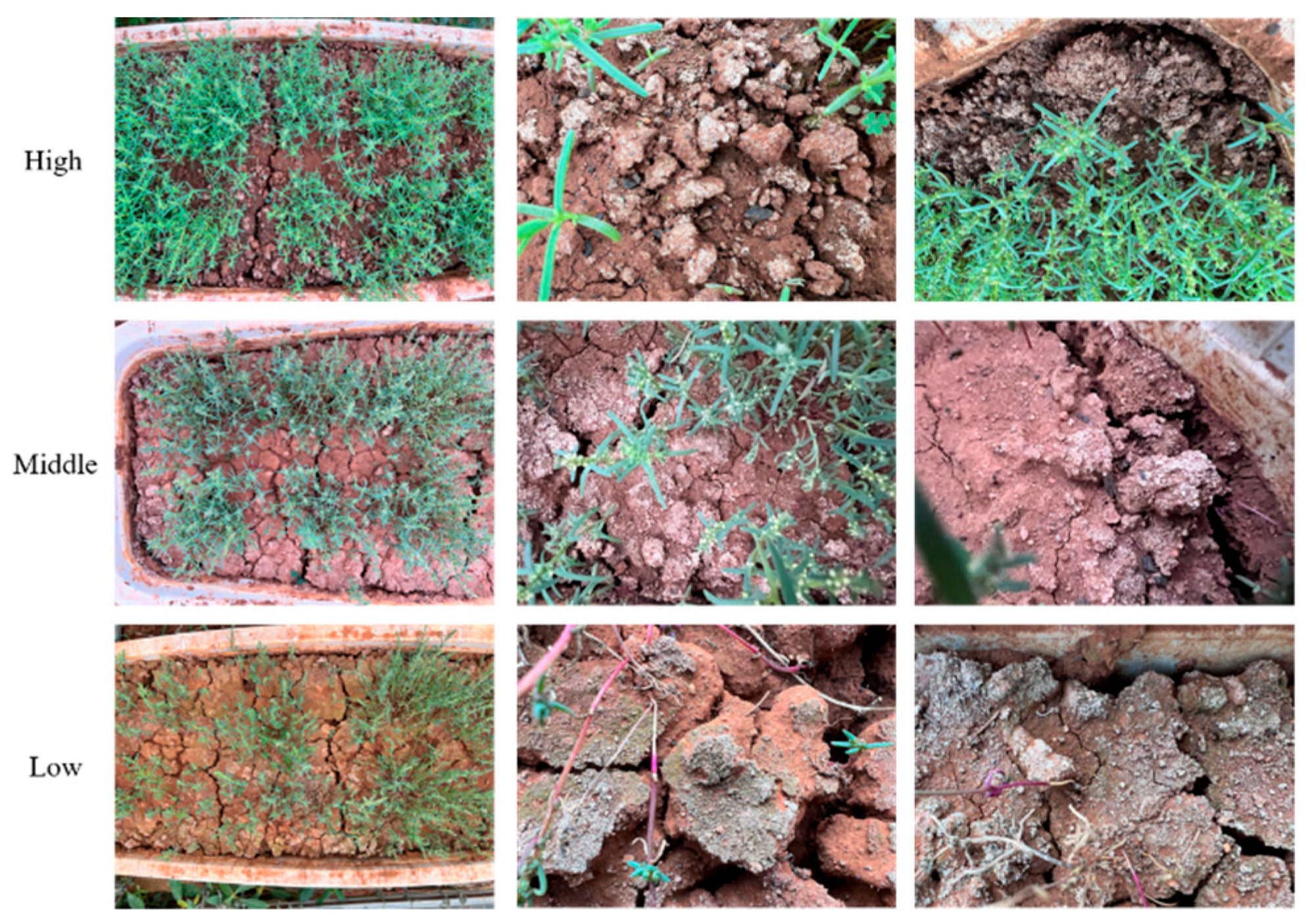
The dataset was collected from a controlled greenhouse experiment conducted at the Chenggong Campus of Kunming University of Science and Technology, Yunnan Province (102.856° E, 24.852° N). Twelve plastic pots (50 L each) were used, and each was filled with 45 kg of sieved soil. To improve drainage, a 1 mm stainless steel mesh was placed at the bottom of each pot, with 5 kg of quartz sand layered beneath it. Soil salinity was manipulated by establishing a gradient through the addition of analytically pure NaCl (purity ≥ 99.5%). The low-salinity group used untreated soil as a control, the medium-salinity group was amended with 90 g NaCl per pot, and the high-salinity group received 180 g NaCl per pot. All soil treatments were thoroughly mixed to ensure uniform salt distribution before loading into the containers. Suaeda glauca was planted in each pot, and four pots were allocated for each salinity treatment (Figure 1). Suaeda glauca is not essential in the classification model, but it simulates the inhomogeneity of the soil surface in real environments, as well as increasing the visual complexity of saline soils. Plants were watered with deionized water every 2–3 days to maintain field water holding capacity and to simulate salt retention effects. Additional NaCl was added after the initial treatment, and watering did not result in significant leaching due to the controlled basin design.

This paper uses camera images to construct a dataset containing 3450 high-resolution (1024 × 1024) soil salinization images, covering three categories of soil salinization images: ‘high’, ‘medium’, and ‘low’. Each category contained 1150 samples, captured from multiple angles and locations in each basin over the same two-month period to account for visual differences, with no adjustment for magnification. The specific information of the dataset is shown in

Table 1. Classification setting of datasets.

	Low	Middle	High	Total
train	850	850	850	2550
validation	200	200	200	600
test	100	100	100	300
total	1150	1150	1150	3450

, which divides the image of each degree of salinization into a training set, a validation set, and a test set. A total of 850 images (2550 in total) of each salinity category were used as the training set, 200 images (600 in total) were used as the validation set, and 100 images (300 in total) were used as the test set. In high-salinity soil, Suaeda glauca grows lusher, resulting in different shapes and sizes of bare soil. In medium-salinity soil, with the improvement of Suaeda glauca, it will become similar to low-salinity soil (original soil), which brings challenges to the collection and classification tasks of datasets. The example of datasets is shown in Figure 2.

In order to improve the generalization performance of the model, the data preprocessing process is a crucial and indispensable step in deep learning applications. This chapter optimizes the generalization ability of the model by integrating various technical means and methods. Specifically, the dynamic size normalization technique is used to map the input image resolution to 224 × 224 by a bilinear interpolation algorithm, and the random rotation technique (between −10 and 10 degrees) is applied to increase the diversity and richness of the data. Considering that the low salinity (original soil) is more similar to the medium salinity soil, in order to improve the classification accuracy, Gaussian blur technology is also used to reduce noise and improve image quality. Finally, the processed image is converted into a tensor and normalized to ensure the consistency and stability of the input dimension of the model. In addition, color conversion is performed, and parameters such as brightness, contrast, and saturation are adjusted to improve the expressiveness and separability of the image. These preprocessing steps enable the model to obtain more accurate, clearer, and valuable image data. We also use the same processed dataset for all the comparison models to ensure fairness and consistency, so as to better evaluate their performance differences.

2.2. Overall Architecture

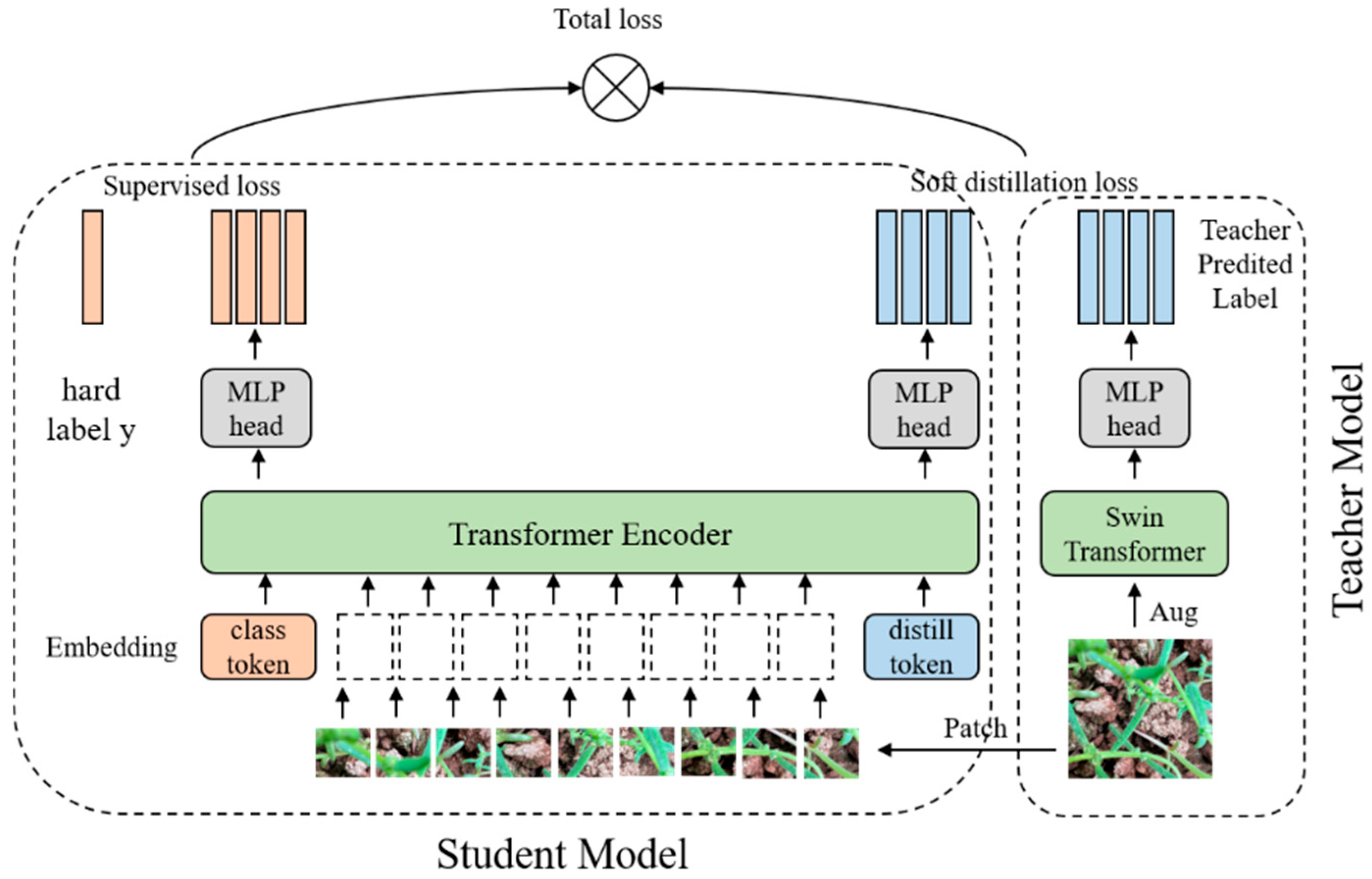
The overall structure of the model will be introduced in this section. The teacher model, designated as Net-T, and the student model, denoted as Net-S, were employed in this study. The teacher model uses the Swin Transformer model, and the student model uses a distillation method to train the dataset. Our improvement is mainly a knowledge distillation of the Swin Transformer model by adding a based-token distillation. Figure 3 shows the overall architecture of Swin-KD. The overall architecture involves training Net-T, followed by distilling its knowledge at a high temperature T to obtain Net-S. The training process of Net-T is straightforward, where the objective function of the high-temperature distillation involves weighting the distill loss (representing the soft target) and the student loss (representing the hard target) as follows: the distillation in this model uses Swin Transformer a teacher network to pass the inductive bias to the student model in a soft way, introducing the assumption of locality by distillation.

2.3. Teacher Model

Swin Transformer is a successful example of applying a sequential data processing approach from natural language processing (NLP) [28] analysis to the field of computer vision [29]. Figure 4 illustrates the overall architecture of the Swin Transformer. Swin Transformer is adopted in our framework as the base model due to its ability to capture both local and global spatial features through hierarchical window-based self-attention. In our implementation, the input image is divided into non-overlapping 4 × 4 patches, which are treated as tokens. These tokens are passed through a series of Swin Transformer blocks with alternating window-based (W-MSA) and shifted window-based (SW-MSA) multi-head self-attention mechanisms. Comparison of the computational volume of MSA and W-MSA:

$$\Omega \left(MSA\right)=4hw{C}^2+2{\left(hw\right)}^{2}C$$

(1)

$$\Omega \left(W\text{-}MSA\right)=4hw{C}^2+2M^{2}hwC$$

(2)

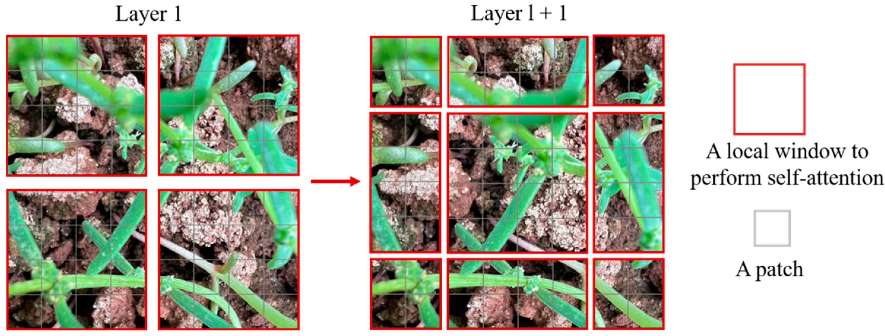
Although W-MSA reduces computational complexity, the non-overlapping windows lack information exchange, so the introduction of a shifted window partition serves to solve the problem of information exchange between disparate windows, which alternates directly between two Swin Transformer Blocks in consecutive Swin Transformer Blocks. This design allows for efficient feature extraction with reduced computational cost while preserving cross-window information exchange. We retain the original four-stage structure of Swin Transformer but later introduce a lightweight variant with knowledge distillation to reduce parameter size and improve inference speed, as described in Section 2.4.

2.3.1. Shifted Window in Teacher Model

Most relevant to our work is the Vision Transformer model [30] and its successors [31,32,33,34]. The groundbreaking work of Vision Transformer (ViT) utilizes the Transformer model architecture directly on non-overlapping medium-sized image blocks for image classification. ViT achieves a remarkable balance between speed and precision in this domain compared to traditional CNN approaches. However, it comes with drawbacks such as low-resolution feature maps and increased complexity due to image size. In contrast, the Swin Transformer exhibits linear complexity and focuses on local interactions. Through empirical observations, it has been found that the Swin Transformer architecture provides a superior trade-off between speed and precision in image classification tasks. The efficient and effective design of the Swin Transformer consistently delivers the highest accuracy across various classification tasks. In summary, Swin Transformer combines the advantages of the local receptive field and hierarchical feature extraction in convolutional neural networks while retaining the global context modeling ability in Transformer and reducing the secondary increase in ViT complexity. This makes the Swin Transformer a powerful visual model for various computer vision tasks.

Swin Transformer adopts a hierarchical architecture that partitions input images into non-overlapping windows and performs self-attention within each window. This window-based attention mechanism significantly reduces computational complexity while preserving local spatial features. To enable long-range dependency modeling, Swin Transformer introduces a shifted window approach, where adjacent layers alternate between standard window attention and shifted window attention, facilitating cross-window information exchange. Unlike ViT, which applies global attention at all layers, Swin Transformer achieves a balance between efficiency and representational power through localized attention and hierarchical feature fusion.

In our implementation, RGB images are first divided into 4 × 4 patches and linearly embedded into tokens. These tokens pass through four stages of Swin Transformer blocks, each responsible for extracting features at progressively coarser spatial resolutions. The sliding window mechanism, combined with multi-scale hierarchical design, enables effective modeling of both fine-grained salt textures and large-scale spatial salinity patterns, which are critical for accurate classification in complex field environments. The sliding window strategy is illustrated in Figure 5.

2.3.2. Self-Attention in the Teacher Model

With the rise in Transformer models, attention mechanisms have gained prominence in computer vision tasks such as classification and segmentation. Unlike traditional convolutional neural networks (CNNs), which rely on fixed local receptive fields and hierarchical layer-wise processing (e.g., ResNet [35]), attention-based models can directly model long-range dependencies across spatial locations. This enables more effective global context integration, which is particularly valuable for complex visual structures. To address the limitations of local feature interaction in CNNs [36], recent studies have introduced attention mechanisms into convolutional architectures, replacing some or all spatial convolutions to enhance contextual awareness and model interpretability [37].

However, attention mechanisms typically incur higher computational costs and memory usage compared to standard convolutions. Transformers, while offering improved accuracy, often suffer from increased inference latency due to memory-intensive operations [38]. To alleviate this, the Swin Transformer introduces a hierarchical structure with non-overlapping local windows and a shifted windowing scheme between layers. This design improves efficiency by reducing redundant computation, enabling better hardware utilization, and achieving a more favorable trade-off between accuracy and complexity. Swin Transformer’s balance of global modeling capacity and computational efficiency makes it a promising backbone for vision tasks that require both fine-grained detail and large-scale spatial reasoning.

2.4. Student Model

Deep learning has achieved remarkable progress in computer vision, speech recognition, and natural language processing. However, the high computational cost of state-of-the-art models remains a major barrier to deployment in resource-constrained environments such as mobile and embedded systems. Knowledge Distillation (KD), first proposed by Hinton et al. [39], offers an effective solution by transferring knowledge from a large, high-performing teacher model to a smaller student model. This allows the student to approximate the performance of the teacher while significantly reducing parameter count and inference cost [40].

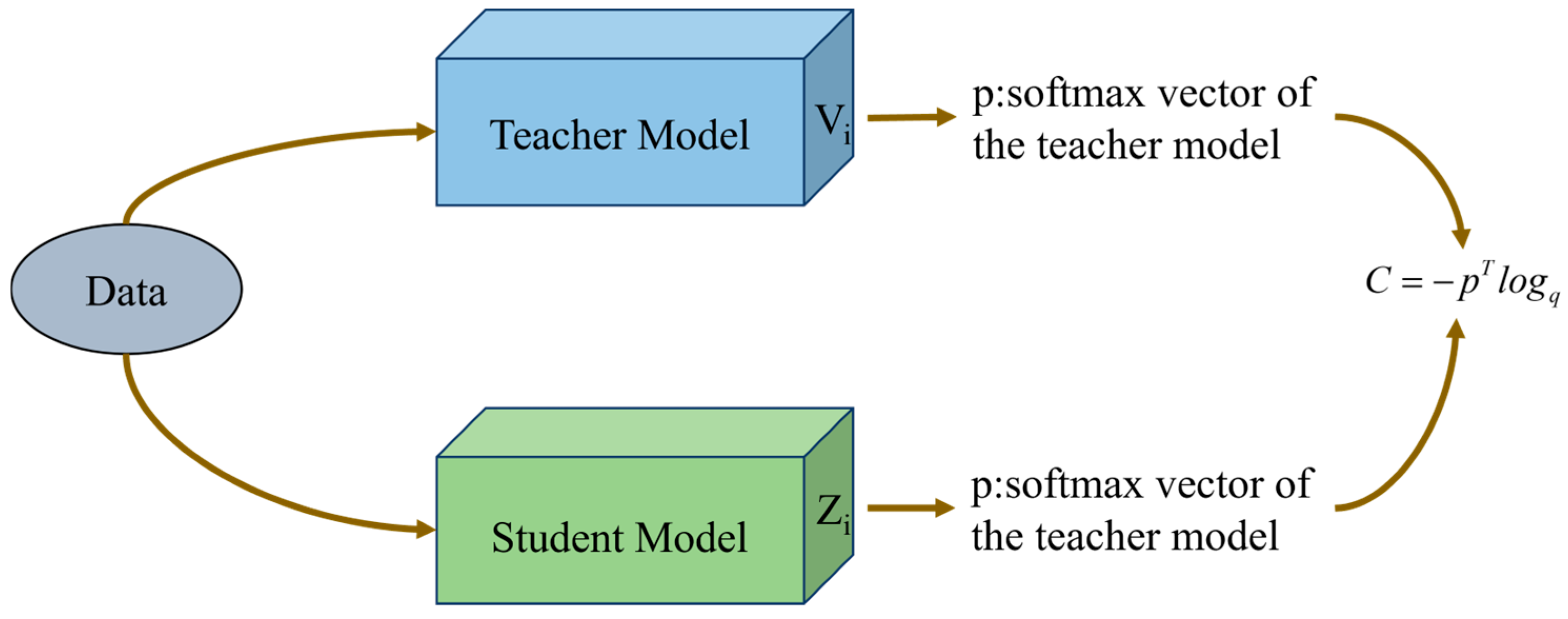
KD has since been widely applied in both vision and language tasks, enabling the development of lightweight yet accurate models. The technique typically involves training the student to match the softened output distributions (soft labels) of the teacher model, generated by applying a temperature-scaled softmax function [41]. This process allows the student to learn the relative confidence levels across classes, beyond what is available from hard ground-truth labels alone [42]. In practice, a hybrid loss function combining both soft and hard labels is used, encouraging the student to learn both the true targets and the teacher’s informative predictions, as shown in Figure 6. In this study, we leverage KD to compress the Swin Transformer by transferring its knowledge to a compact student model, Swin-KD, thereby maintaining high classification performance while improving inference speed and reducing computational demands.

Based-Token Distillation in the Student Model

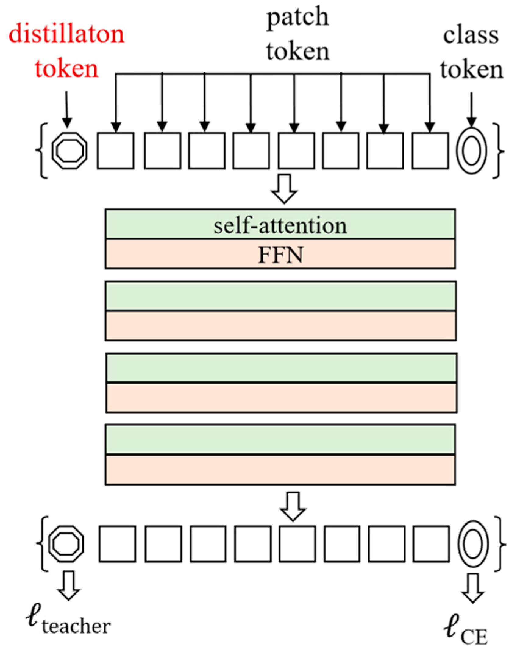
In this study, we adopt a token-based knowledge distillation strategy within a full Transformer architecture. Specifically, Swin Transformer is used as the teacher model due to its strong performance in classification tasks. The student model, Swin-KD, is trained to mimic the predictions of the teacher through the introduction of a Distillation Token alongside the standard Class Token. These tokens are jointly processed in the self-attention layers, where the Class Token is supervised by ground-truth labels, while the Distillation Token learns to match the soft predictions of the teacher model [43].

This dual-token design allows the student to simultaneously learn from hard targets and soft targets, enhancing its generalization ability. Compared to traditional training with hard labels alone, knowledge distillation enables the student model to capture the relative confidence distribution across all classes, which provides richer supervisory signals. Furthermore, since both tokens participate in attention-based interactions throughout the Transformer layers, the student can better align its internal representations with those of the teacher.

The use of token-based distillation not only simplifies the distillation process—without requiring additional attention, map matching, or feature alignment—but also ensures efficient training and strong performance under a compact model design. The overall loss function includes both cross-entropy loss and distillation loss, with the Distillation Token playing a central role in guiding the knowledge transfer.

Distillation loss: There are two types of distillation: soft distillation and hard distillation. Soft distillation minimizes the Kullback–Leibler loss of softmax for both teacher and student models. The soft distillation equation is shown in Formula (3).

$${\mathcal{l}}_{global}=\left(1-\lambda \right){\mathcal{l}}_{CE}\left(\psi \left(Z_{\mathrm{s}}\right),\mathrm{y}\right)+\lambda {\tau }^{2}KL\left(\psi \left(Z_{\mathrm{s}}/\tau \right),\psi \left({\mathrm{Z}}_{\mathrm{t}}/\tau \right)\right)$$

(3)

Equation (3) defines $Z_t$ as the logarithm of the teacher model and $Z_s$ as the logarithm of the student model. KL represents the Kullback–Leibler divergence and balances the loss between the Kullback–Leibler divergence (KL) and the loss of cross-entropy (LCE) of the ground truth label y. The softmax function is denoted as $\mathsf{\lambda }$, and the distillation temperature is denoted as $\tau$.

Introducing a distillation variant, the teacher’s hard decision is considered the true value label, where the function is applied to determine the teacher’s hard decision. The distillation of this hard label is represented as follows, with CE indicating cross entropy:

$${\mathcal{l}}_{\mathrm{global}}^{\mathrm{hardDistill}}={\displaystyle \frac{1}{2}}{\mathcal{l}}_{\mathrm{CE}}\left(\psi \left({\mathrm{Z}}_{\mathrm{s}}\right),\mathrm{y}\right)+{\displaystyle \frac{1}{2}}{\mathcal{l}}_{\mathrm{CE}}\left(\psi \left({\mathrm{Z}}_{\mathrm{s}}\right),{\mathrm{y}}_{\mathrm{t}}\right)$$

(4)

To facilitate effective knowledge transfer, we employ both soft and hard distillation strategies in training the student model. For soft distillation, we use the Kullback–Leibler divergence (KL Loss) between the softmax outputs of the teacher and student networks. For hard distillation, we compute cross-entropy loss (CE Loss) between the student output and the teacher’s predicted label. Additionally, label smoothing is applied to the ground-truth labels, assigning a probability of 1-ε to the correct class and distributing the remaining ε = 0.1 uniformly across the other classes, which helps improve generalization and regularize hard targets [44].

Our approach introduces a Distillation Token into the Transformer architecture, alongside the standard Class Token and patch embeddings (see Figure 7). This token follows the same attention-based interaction and propagation as the Class Token and is appended to the input sequence. While the Class Token is supervised using ground-truth labels, the Distillation Token is optimized against the teacher’s output, forming the basis of the distillation loss. This token-based design enables the student model to simultaneously learn from true labels and the softened predictions of the teacher, within a unified Transformer framework. Interestingly, we observe that the Distillation Token and Class Token evolve differently across layers. The average cosine similarity between their representations is initially low (0.06), indicating their distinct roles in early stages. However, this similarity progressively increases and reaches 0.93 in the final layer, suggesting successful integration of complementary supervision signals during training.

2.5. Evaluation Metrics

In this paper, the accuracy, precision, recall, and F1 score indicators commonly used in image classification algorithm research are used for evaluation. The above four indicators are all that the larger the value, the better the classification performance of the model. Accuracy refers to the ratio of the number of sample books correctly classified by the classifier to the total number of samples for a given test dataset, that is, the proportion of correct model judgment, which is the most intuitive indicator of model performance. Its calculation is shown in Formula (5):

$$Accuracy=(TP+TN)/(TP+TN+FP+FN)$$

(5)

The accuracy rate represents the actual proportion of positive samples in the samples judged as positive by the model. Its calculation is shown in Formula (6):

$$Precision=TP/(TP+FP)$$

(6)

The recall rate indicates the proportion of samples that are actually positive, judged by the model as positive samples, which is complementary to the accuracy rate. Its calculation is shown in Formula (7):

$$Recall=TP/(TP+FN)$$

(7)

Precision and recall are a pair of contradictory evaluation indicators. Usually, when the precision is high, the recall rate is often low. The F1 score index takes into account the accuracy and recall rate. Its calculation is shown in Formula (8):

$$F1score=2/(2TP+FP+FN)$$

(8)

In the field of deep learning, model parameters refer to the number of adjustable parameters, such as weights and biases, that need to be learned in deep neural networks. The number of model parameters is an important index to evaluate the size and complexity of the model, which is usually closely related to the capacity and generalization ability of the model. The size of the model parameters directly affects the storage requirements and computing requirements of the model. The larger the parameters are, the higher the complexity of the model is, and the stronger the expression ability of the model is in theory. However, it also leads to the need for more memory and computing resources in the training and reasoning process of the model, and over-fitting may occur, that is, the model performs well on the training set but performs poorly on the test set. Therefore, when designing deep learning models, researchers usually consider how to reduce the number of parameters of the model as much as possible while maintaining good performance, so as to improve the efficiency and versatility of the model, which requires a balance between the complexity and generalization ability of the model.

3. Results

3.1. Implementation Details

This experiment was run under the Unbantu 22.04.2 LTS operating system using the PyTorch 1.9.0 and CUDA 1.1.0 frameworks. The hyperparameter setting is crucial for achieving good performance in model training. The initial learning rate is set to 1 × 10⁻⁵ (i.e., 0.00001), and it decreases exponentially after 20 rounds of training until the minimum learning rate of 1 × 10⁻⁹ is reached. The weight_decay is set to 1 × 10⁻⁴ and the random seed is set to 42. In addition, after many experiments and reference-related research, the AdamW [45] optimizer was finally used to train the model. The data for each round of training (batch _ size) is 64, and the entire model is trained for 40 rounds. Finally, the alpha was set to 0.5 for distillation, and the distillation temperature was set to 1 after the experiment. By setting these hyperparameters, the model can be trained quickly, stably, and efficiently, so as to obtain better classification results.

To ensure a fair and unbiased evaluation, the dataset was strictly partitioned into three mutually exclusive subsets: training, validation, and test sets. The training set was used to optimize model parameters through learning, while the validation set served to monitor performance during training and guide hyperparameter tuning. The test set was reserved exclusively for final performance evaluation after all training and tuning procedures were completed. This setup avoids data leakage and ensures that the reported results reflect the model’s true generalization ability.

3.2. Image Classification on the Saline Soil Dataset

To evaluate the classification performance, we compared Swin-KD with several mainstream models, including Swin Transformer, ResNet152, and VGG16 [46] using accuracy, F1-score, recall, loss, and parameter count as key metrics. As shown in Figure 8, the accuracy of Swin-KD, Swin Transformer, ResNet152, and VGG16 on the verification set was 96.3%, 96%, 95.5%, and 95.3%, respectively. Among the compared models, VGG16 exhibited the lowest accuracy (95.3%) and the most pronounced training fluctuations, indicating its limited ability to capture subtle visual distinctions between low- and medium-salinity areas. ResNet152 converged rapidly and performed stably (95.5%) due to its deep residual architecture, which effectively models salinity gradients, especially in high-salinity zones. Swin Transformer achieved higher accuracy (96.0%) with better convergence, benefiting from its hierarchical self-attention mechanism that captures local spatial context. The proposed Swin-KD model achieved the highest accuracy (96.3%) and demonstrated remarkable stability throughout training. By integrating token-based knowledge distillation, it effectively enhances feature extraction while reducing parameters. This is particularly advantageous in complex salinity scenarios characterized by spatial fragmentation and vegetative occlusion. Moreover, Swin-KD maintained accuracy above 90% after only 15 epochs, indicating both training efficiency and strong generalization. Overall, Swin-KD outperforms baseline models in both precision and robustness, making it well-suited for real-world soil salinity classification tasks.

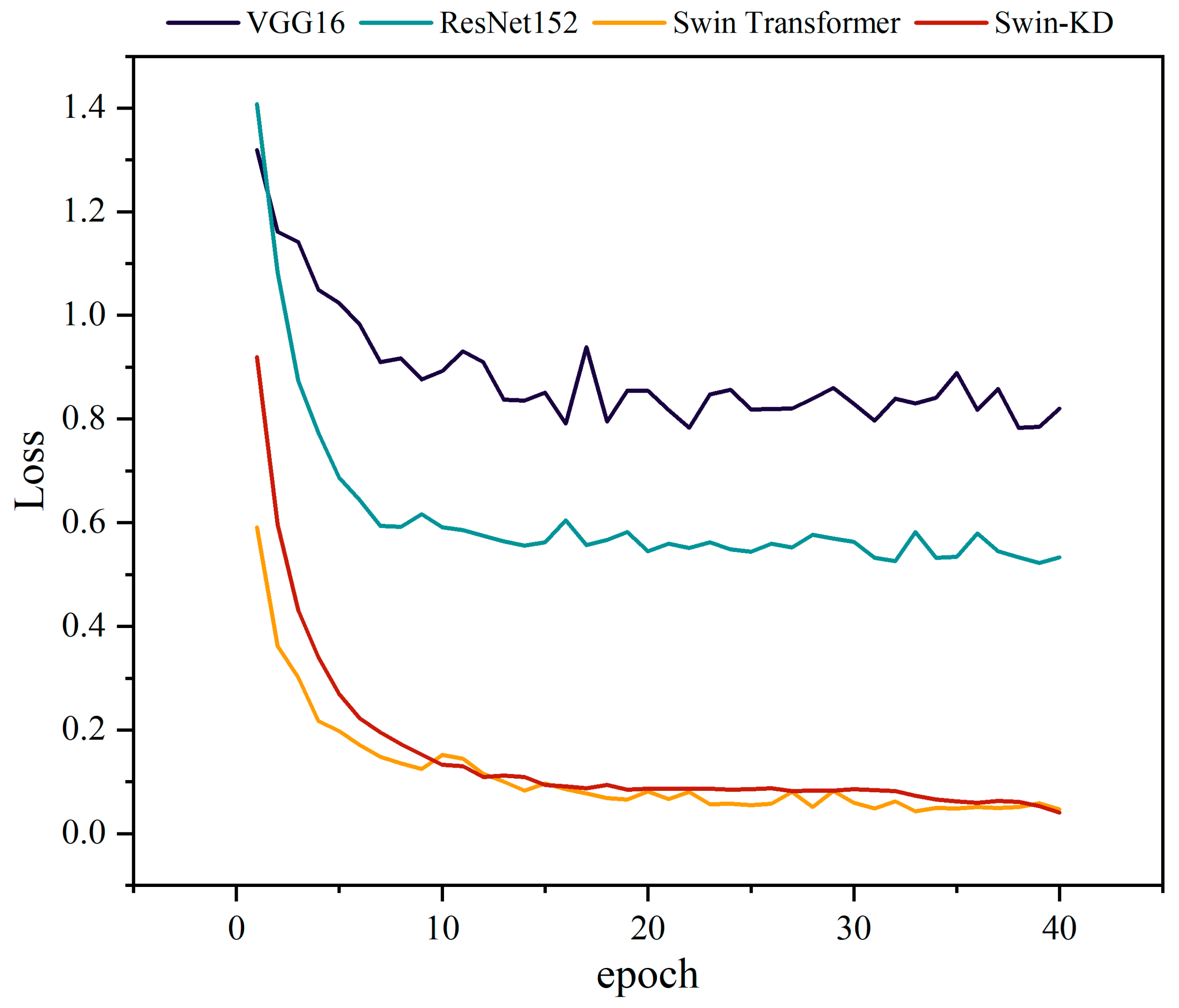
Based on the changes in loss values over 40 training epochs (Figure 9), the models exhibited varying levels of convergence and optimization ability. The ResNet152 model demonstrated a rapid initial decline in loss, stabilizing below 0.6 after 10 epochs and fluctuating between 0.5 and 0.6 thereafter. This plateau suggests limitations in modeling small or edge saline regions due to their fixed receptive field. In contrast, VGG16 exhibited the slowest convergence, with loss values remaining around 0.8 throughout training. Its sequential convolution layers struggle to capture low-contrast differences between salt and soil background, leading to insufficient spatial sensitivity and slower learning progression. In comparison, both Swin Transformer and Swin-KD achieved significantly lower loss values—dropping below 0.2 within the first five epochs and ultimately reaching values under 0.05. Swin Transformer displayed rapid early decline with minor fluctuations, attributed to its hierarchical self-attention mechanism, which effectively captures multi-scale spatial patterns and relationships through local and shifted windows. The Swin-KD model further improved stability, showing a sharp initial decline followed by a smooth, fluctuation-free downward trend, reflecting superior optimization capacity. This consistent loss reduction highlights Swin-KD’s robust adaptability to complex training data. Overall, Swin-KD outperformed the other models in convergence speed, optimization efficiency, and training stability, underscoring its suitability for precise salinity classification under challenging visual conditions.

Table 2. Performance test results of models.

Models	Recall (%)			F1_Score (%)			Precision (%)			Accuracy (%)	Params (M)
	Low	Middle	High	Low	Middle	High	Low	Middle	High
AlexNet	94.97	83.33	86.30	96.92	82.44	85.52	98.95	81.57	84.75	88.24	61.12
DensenNet	100.00	93.01	88.58	98.27	90.81	91.94	96.60	88.71	95.56	93.70	14.16
ResNet152	100.00	87.63	95.89	99.25	91.06	93.54	98.51	94.76	91.30	94.70	58.15
Efficiennet	99.49	85.48	94.06	98.75	89.32	91.35	98.01	93.52	88.79	93.21	145.00
InceptionV3	99.49	87.09	89.04	98.75	87.09	89.65	98.01	87.09	90.27	91.88	24.36
VGG16	100.00	88.17	91.78	98.27	89.86	91.78	96.60	91.62	91.78	93.37	117.51
VGG19	98.49	87.09	92.23	98.49	88.28	91.19	98.49	89.50	90.17	92.71	139.59
MobileNetV3	98.49	88.09	89.04	98.25	88.09	89.15	98.01	88.09	89.27	91.68	5.40
EfficientFormer	99.49	88.14	95.89	99.04	91.06	93.43	98.61	94.86	91.10	94.60	13.80
Vision Transformer	92.49	5.31	16.27	50.45	5.38	14.95	34.68	5.45	13.82	38.63	85.80
Swin Transformer	100.00	94.52	96.70	96.12	96.10	96.10	98.52	95.71	95.31	96.00	27.50
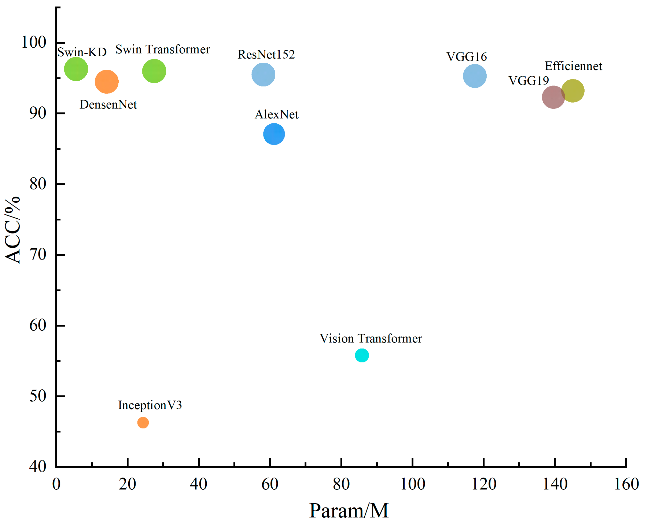
Swin-KD	100.00	94.06	96.93	99.44	95.43	96.61	98.89	96.00	96.31	96.30	5.53

compares the proposed Swin-KD model with other backbone networks, including Transformer-based and ConvNet-based architectures, using evaluation metrics such as recall, precision, F1 score, overall accuracy, and parameter count. While most models showed good performance across multiple metrics, notable differences were observed in class-wise recognition. Many models struggled to classify moderately saline soils, with recall rates often falling below 90 percent, indicating a higher misclassification rate in this category. In contrast, AlexNet performed well in low-salinity soil classification, achieving high precision, but its overall robustness was limited. Both Swin Transformer and Swin-KD demonstrated strong and consistent performance across all salinity levels. Swin Transformer achieved a precision of 95 percent, while Swin-KD further improved to 96.3 percent. In terms of F1 score, Swin-KD showed a slight drop of 0.67 percent compared to Swin Transformer on moderate salinity samples but remained competitive overall. DensenNet, ResNet152, VGG16, and VGG19 also delivered high recognition accuracy. Swin-KD achieved the highest classification accuracy of 96.3 percent while maintaining the lowest parameter count at 5.53 million. In comparison, InceptionV3 had 24.36 million parameters, and EfficientNet, VGG16, VGG19, and Vision Transformer models all had relatively larger sizes. Figure 10 illustrates that Swin-KD achieves a favorable trade-off between model complexity and performance. The combination of lightweight design and accurate classification highlights the advantages of introducing knowledge distillation into the Swin Transformer architecture.

Table 3. Confidence interval of the model.

Model	Acc (%)	Confidence Interval (95%)
AlexNet	88.24	(0.8182, 0.9466)
DensenNet	93.70	(0.8897, 0.9843)
ResNet152	94.70	(0.9044, 0.9896)
Efficiennet	93.21	(0.8831, 0.9811)
InceptionV3	91.88	(0.8642, 0.9734)
VGG16	93.37	(0.8856, 0.9818)
VGG19	92.71	(0.8768, 0.9774)
MobileNetV3	91.68	(0.8627, 0.9709)
EfficientFormer	94.60	(0.9017, 0.9903)
Vision Transformer	38.63	(0.2915, 0.4811)
Swin Transformer	96.00	(0.9215, 0.9985)
Swin-KD	96.30	(0.9262, 0.9998)

shows the classification accuracy and 95% confidence intervals for different models. Swin-KD achieves the highest accuracy (96.30%) with a narrow and high confidence interval (0.9262–0.9998), indicating both strong performance and high statistical reliability. Swin Transformer ranks second (96.00%), confirming the strength of transformer-based architectures in saline soil classification. EfficientFormer and ResNet152 also perform well (>94%), showing a good balance between depth and generalization. In contrast, traditional CNNs like AlexNet and MobileNetV3 exhibit lower accuracy and wider intervals, suggesting limited robustness. Notably, Vision Transformer shows poor performance (38.63%), with a low and wide confidence interval, likely due to its lack of inductive bias and insufficient adaptation to small-scale datasets. Overall, Swin-KD demonstrates not only superior accuracy but also more stable performance across test samples.

In saline soil classification, inference efficiency is crucial for real-time monitoring. As shown in

Table 4. Inference time off per hundred images for different models (s).

Model	Test1	Test2	Test3	Test4	Test5	Average
AlexNet	12.16	11.07	12.34	12.36	11.23	11.832
DensenNet	11.88	11.61	11.89	11.83	11.66	11.774
ResNet152	12.33	11.20	12.24	12.32	11.12	11.842
Efficiennet	12.25	11.05	12.36	11.93	10.98	12.742
InceptionV3	12.51	11.30	12.36	12.46	11.27	11.980
VGG16	13.13	11.87	13.40	13.26	12.05	12.742
VGG19	13.07	12.01	13.44	13.27	11.84	12.726
Vision Transformer	13.02	11.77	12.91	13.07	11.71	12.496
Swin Transformer	12.52	11.22	12.60	12.21	11.28	11.966
Swin-KD	12.11	10.90	11.97	12.19	10.75	11.584

, Swin-KD achieves the fastest inference time (11.584 s per 100 images), benefiting from its lightweight architecture guided by knowledge distillation. By inheriting spatial priors from the teacher model, Swin-KD can accurately focus on salt-affected regions using fewer layers. Its local attention mechanism further concentrates computation on relevant patches, while reusing feature templates reduces redundant operations. In contrast, ResNet152 and DenseNet, though structurally robust, lack adaptation to salinity-specific patterns, resulting in slower inference. VGG16 performs worst due to its large fully connected layers and inability to leverage spatial regularity. Overall, Swin-KD demonstrates a superior speed–accuracy tradeoff, supporting its suitability for field deployment.

In order to prove the generalization performance of the algorithm, we have performed experiments on the public dataset ImageNet-1K.

Table 5. Comparison of Acc and Param metrics for different classification models on ImageNet-1K.

Model	Acc (%)	Param (M)
AlexNet	57.2	61.0
DensenNet	74.9	8.0
ResNet152	76.2	60.2
EfficientNet	77.1	5.0
InceptionV3	77.9	23.8
VGG16	71.3	138.4
VGG19	71.6	143.7
MobileNetV3	75.2	5.4
EfficientFormer	81.0	13.8
Vision Transformer	77.9	86.5
Swin Transformer	81.3	27.5
Swin-KD	81.8	5.53

compares the classification accuracy (Acc) and model complexity (measured by parameter count) of various architectures on the ImageNet-1K dataset. In order to prove the generalization performance of the algorithm, we have conducted experiments on the public dataset ImageNet-1K. Table 5 compares the classification accuracy (Acc) and model complexity (measured by parameter count) of various architectures on the ImageNet-1K dataset. Traditional CNN models, such as VGG16 and VGG19, show relatively low accuracies of 71.3% and 71.6%, respectively, despite having very large parameter sizes of 138.4M and 143.7M. This indicates inefficiency in representation. In contrast, lightweight architectures like EfficientNet and MobileNetV3 achieve higher accuracies of 77.1% and 75.2%, respectively, with significantly fewer parameters of 5.0M and 5.4M, reflecting better parameter efficiency. Transformer-based models also show strong performance, with the Swin Transformer reaching 81.3% accuracy with 27.5M parameters. Notably, the proposed Swin-KD model achieves the highest accuracy of 81.8% with only 5.53M parameters, outperforming both the Swin Transformer and other lightweight models. This highlights the effectiveness of knowledge distillation in enhancing performance while maintaining a low computational cost, making Swin-KD highly suitable for resource-constrained deployment scenarios without sacrificing accuracy.

3.3. Results Visualization

Figure 11 presents the confusion matrices of four models on the test set, revealing not only performance differences but also structural limitations in handling varying degrees of soil salinity. All models achieved perfect classification on low-salinity (original) soil, indicating strong discrimination of non-salinized regions. However, classification accuracy dropped for medium- and high-salinity soils, exposing each model’s weaknesses. ResNet152 misclassified 17 high-salinity samples as medium-salinity, reflecting its limited ability to capture spatial transitions due to its fixed receptive field and lack of fine-grained edge sensitivity. VGG16, though slightly better, showed misclassifications likely caused by sensitivity to lighting artifacts and specular reflection, highlighting its limited robustness in complex imaging conditions. The Swin Transformer improved classification through multi-scale attention but still misjudged boundary zones, suggesting insufficient local continuity modeling despite global attention. Swin-KD achieved the highest accuracy, reducing misclassifications to only four high-salinity samples, and demonstrated better handling of ambiguous regions. However, its reliance on distilled knowledge raises questions about its adaptability to unseen data distributions. These results suggest that while transformer-based models outperform CNNs in salinity classification, challenges remain in boundary detection, scale sensitivity, and real-world generalizability.

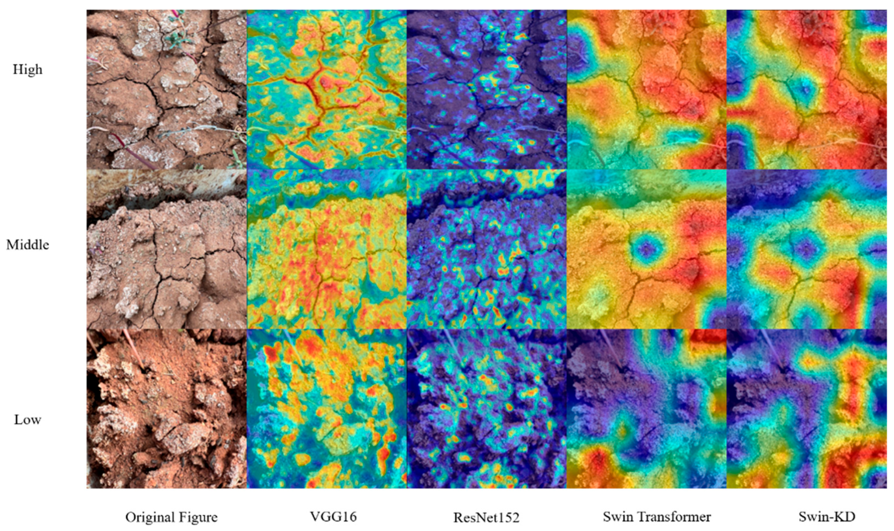
Class activation mapping (CAM) was used to critically assess how different models attend to salient features in saline soil images (Figure 12). VGG16 exhibited scattered and misaligned activations, often focusing on background noise due to pooling-induced loss of spatial detail. ResNet152 showed improved localization but struggled with small-scale salt patches, likely due to its fixed convolutional kernel size. Swin Transformer better captured concentrated salt areas through self-attention but showed weak responses near saline boundaries, suggesting limited local continuity modeling. Swin-KD, enhanced by knowledge distillation, focused more accurately on ecologically relevant features such as gullies and salt crusts, and effectively suppressed irrelevant reflectance artifacts. However, its reliance on teacher priors may reduce generalizability in unseen environments. Overall, while attention-based models improve spatial interpretability, challenges remain in boundary detection, noise robustness, and ecological transferability.

In summary, the Swin-KD model can improve the classification accuracy of soil salinity, significantly improve the model size, and better meet practical production needs regarding classification efficiency and generalization performance. The Swin-KD model has significantly fewer parameters than others, with just 5.3 M. Considering model accuracy, our proposed model also outperforms other models slightly, achieving a 96.3% accuracy. From the class activation mapping diagram, our proposed model focuses more on soil gullies and salinization of the soil surface. Therefore, our model is generally superior in classifying and identifying the degree of soil salinization.

4. Discussion

Although the proposed model achieves strong performance on our saline soil classification task, there are still aspects that warrant further improvement. One concern is the potential risk of representation over-smoothing, which may occur due to the limited number of stacked layers. As the model deepens, token representations—including those of additional tokens—tend to become increasingly similar, potentially weakening discriminative capacity. While increasing the hidden dimensionality could mitigate this issue, it comes at the cost of significantly larger parameter sizes. A more efficient alternative would be to diversify the attention mechanism, such as introducing linear transformations before and after the SoftMax operation in the attention heads to enhance inter-token variability and improve information flow.

In addition to architectural considerations, the dataset design also imposes limitations on generalization. The effectiveness of machine learning models for soil salinity classification heavily depends on the quality and size of the image dataset used for training. Research has shown that deep learning models, such as convolutional neural networks (CNNs), require large datasets to perform well in image classification tasks [35]. In this study, the dataset of 3450 images (1150 images per salinity group) is relatively large compared to some earlier studies, which used smaller datasets of around 1000 images for similar tasks [42]. While this dataset size appears sufficient for training robust models, it is important to recognize that the inclusion of additional factors, such as variations in soil types or plant species, could enhance the model’s generalizability and accuracy. However, the current dataset has not been validated under diverse environmental conditions, limiting its generalizability. All images were collected during daylight hours, and the model has not been tested under artificial lighting or nighttime scenarios. Furthermore, robustness against noise, occlusion, and lighting variation has not yet been evaluated, despite the model’s strong performance in terms of accuracy, precision, recall, and F1-score. Although different subsets of images were used in training, validation, and testing, all images came from the same set of 12 soil pots, which limits the diversity of the dataset. A larger, independently sourced image dataset from different batches or fields would help address potential overfitting issues and improve the model’s generalization across different environments. Future work should focus on expanding the dataset to include diverse environmental conditions and additional factors, ensuring a more comprehensive evaluation of the model’s robustness.

Another important consideration is the ecological realism of the experimental setup. Although the use of NaCl-treated potted soil offers a controlled method for simulating salinity, it does not fully capture the complexity of naturally saline soils, which often feature heterogeneous structures and diverse ionic compositions. This simplification may limit the model’s applicability in large-scale or field-level deployments. Furthermore, the current classification scheme—dividing salinity into three levels (low, medium, high)—aligns with commonly used agricultural thresholds, such as those recommended by the FAO. While this categorization ensures computational efficiency and supports rapid assessment applications, future studies can explore finer-grained classifications (e.g., 5–7 levels) by leveraging more diverse and extensive datasets. To improve ecological validity and practical applicability, subsequent research should also incorporate naturally salinized soils from different geographic regions and evaluate the model’s robustness in real-world field conditions.

Traditional methods for assessing soil salinity often rely on physical soil samples and laboratory analysis, such as measuring the electrical conductivity (EC) or ion concentration. These methods, while accurate, can be time-consuming, labor-intensive, and may not provide real-time or large-scale data [47]. In contrast, the approach used in this study, based on image-based analysis of the soil–plant system, offers a non-invasive and rapid way to assess soil salinity. By leveraging the visual characteristics of the soil surface and plant growth under varying salinity conditions, this approach allows for continuous monitoring of soil salinity without disturbing the soil or plants. Remote sensing technologies, such as satellite or UAV-based imagery, have also been employed for soil salinity assessment [48]. These methods provide spatially distributed data, which is crucial for large-scale assessments. However, they often struggle with resolution limitations, particularly in areas with fine-scale variations in salinity. The camera-based method used here provides a higher level of detail with images captured at much finer spatial scales, enhancing the ability to detect subtle salinity-induced changes in soil surface texture and plant growth.

5. Conclusions

In this study, we propose a lightweight classification model, Swin-KD, based on the Swin Transformer architecture with token-based knowledge distillation. The model effectively reduces the parameter count from 27.5M to 5.53M while improving classification accuracy from 96.0% to 96.3% on the saline soil dataset. These results demonstrate that the proposed distillation strategy enhances both efficiency and performance, making the model more suitable for resource-constrained environments and real-time agricultural monitoring. By enabling faster and more accurate identification of soil salinity levels, the Swin-KD model contributes to the development of intelligent, data-driven approaches for precision agriculture.

References

1. Wang, J.; Ding, J.; Yu, D.; Ma, X.; Zhang, Z.; Ge, X.; Teng, D.; Li, X.; Liang, J.; Lizaga, I.; et al. Capability of Sentinel-2 MSI Data for Monitoring and Mapping of Soil Salinity in Dry and Wet Seasons in the Ebinur Lake Region, Xinjiang, China. Geoderma 2019, 353, 172–187. [Google Scholar] [CrossRef]
2. Li, J.; Gao, Y.; Zhang, X.; Tian, P.; Li, J.; Tian, Y. Comprehensive Comparison of Different Saline Water Irrigation Strategies for Tomato Production: Soil Properties, Plant Growth, Fruit Yield and Fruit Quality. Agric. Water Manag. 2019, 213, 521–533. [Google Scholar] [CrossRef]
3. Chen, H.; Tao, L.; Shi, J.; Han, X.; Cheng, X. Exogenous Salicylic Acid Signal Reveals an Osmotic Regulatory Role in Priming the Seed Germination of Leymus Chinensis under Salt-Alkali Stress. Environ. Exp. Bot. 2021, 188, 104498. [Google Scholar] [CrossRef]
4. Zhang, K.; Chang, L.; Li, G.; Li, Y. Advances and Future Research in Ecological Stoichiometry under Saline-Alkali Stress. Environ. Sci. Pollut. R. 2023, 30, 5475–5486. [Google Scholar] [CrossRef] [PubMed]
5. Bannari, A.; El-Battay, A.; Bannari, R.; Rhinane, H. Sentinel-MSI VNIR and SWIR Bands Sensitivity Analysis for Soil Salinity Discrimination in an Arid Landscape. Remote Sens. 2018, 10, 855. [Google Scholar] [CrossRef]
6. Zhang, Z.; Li, X.; Ren, J.; Zhou, S. Study on the Drying Process and the Influencing Factors of Desiccation Cracking of Cohesive Soda Saline-Alkali Soil in the Songnen Plain, China. Agriculture 2023, 13, 1153. [Google Scholar] [CrossRef]
7. Escorcia-Gutierrez, J.; Gamarra, M.; Soto-Diaz, R.; Pérez, M.; Madera, N.; Mansour, R.F. Intelligent Agricultural Modelling of Soil Nutrients and pH Classification Using Ensemble Deep Learning Techniques. Agriculture 2022, 12, 977. [Google Scholar] [CrossRef]
8. Padmapriya, J.; Sasilatha, T. Deep Learning Based Multi-Labelled Soil Classification and Empirical Estimation toward Sustainable Agriculture. Eng. Appl. Artif. Intell. 2023, 119, 105690. [Google Scholar] [CrossRef]
9. Lanjewar, M.G.; Gurav, O.L. Convolutional Neural Networks Based Classifications of Soil Images. Multimed. Tools Appl. 2022, 81, 10313–10336. [Google Scholar] [CrossRef]
10. Ferrer-Ferrer, M.; Ruiz-Hidalgo, J.; Gregorio, E.; Vilaplana, V.; Morros, J.R.; Gené-Mola, J. Simultaneous Fruit Detection and Size Estimation Using Multitask Deep Neural Networks. Biosyst. Eng. 2023, 233, 63–75. [Google Scholar] [CrossRef]
11. Mia, S.; Tanabe, R.; Habibi, L.N.; Hashimoto, N.; Homma, K.; Maki, M.; Matsui, T.; Tanaka, T.S.T. Multimodal Deep Learning for Rice Yield Prediction Using UAV-Based Multispectral Imagery and Weather Data. Remote Sens. 2023, 15, 2511. [Google Scholar] [CrossRef]
12. Lu, J.; Tan, L.; Jiang, H. Review on Convolutional Neural Network (CNN) Applied to Plant Leaf Disease Classification. Agriculture 2021, 11, 707. [Google Scholar] [CrossRef]
13. Hasan, A.S.M.M.; Sohel, F.; Diepeveen, D.; Laga, H.; Jones, M.G.K. A Survey of Deep Learning Techniques for Weed Detection from Images. Comput. Electron. Agric. 2021, 184, 106067. [Google Scholar] [CrossRef]
14. Moazzam, S.I.; Nawaz, T.; Qureshi, W.S.; Khan, U.S.; Tiwana, M.I. A W-Shaped Convolutional Network for Robust Crop and Weed Classification in Agriculture. Precis. Agric. 2023, 24, 2002–2018. [Google Scholar] [CrossRef]
15. Farrell, M.; Leizica, E.; Gili, A.; Noellemeyer, E. Identification of Management Zones with Different Potential Moisture Availability for Sustainable Intensification of Dryland Agriculture. Precis. Agric. 2023, 24, 1116–1131. [Google Scholar] [CrossRef]
16. De Castro Pereira, R.; Hirose, E.; Ferreira De Carvalho, O.L.; Da Costa, R.M.; Borges, D.L. Detection and Classification of Whiteflies and Development Stages on Soybean Leaves Images Using an Improved Deep Learning Strategy. Comput. Electron. Agric. 2022, 199, 107132. [Google Scholar] [CrossRef]
17. Waheed, A.; Goyal, M.; Gupta, D.; Khanna, A.; Hassanien, A.E.; Pandey, H.M. An Optimized Dense Convolutional Neural Network Model for Disease Recognition and Classification in Corn Leaf. Comput. Electron. Agric. 2020, 175, 105456. [Google Scholar] [CrossRef]
18. Yan, C.; Li, Z.; Zhang, Z.; Sun, Y.; Wang, Y.; Xin, Q. High-Resolution Mapping of Paddy Rice Fields from Unmanned Airborne Vehicle Images Using Enhanced-TransUnet. Comput. Electron. Agric. 2023, 210, 107867. [Google Scholar] [CrossRef]
19. Hayıt, T.; Erbay, H.; Varçın, F.; Hayıt, F.; Akci, N. The Classification of Wheat Yellow Rust Disease Based on a Combination of Textural and Deep Features. Multimed. Tools Appl. 2023, 82, 47405–47423. [Google Scholar] [CrossRef]
20. Paul, S.G.; Biswas, A.A.; Saha, A.; Zulfiker, S.; Ritu, N.A.; Zahan, I.; Rahman, M.; Islam, M.A. A Real-Time Application-Based Convolutional Neural Network Approach for Tomato Leaf Disease Classification. Array 2023, 19, 100313. [Google Scholar] [CrossRef]
21. Kumar, V.S.; Jaganathan, M.; Viswanathan, A.; Umamaheswari, M.; Vignesh, J. Rice Leaf Disease Detection Based on Bidirectional Feature Attention Pyramid Network with YOLO v5 Model. Environ. Res. Commun. 2023, 5, 065014. [Google Scholar] [CrossRef]
22. Sunil, C.K.; Jaidhar, C.D.; Patil, N. Tomato Plant Disease Classification Using Multilevel Feature Fusion with Adaptive Channel Spatial and Pixel Attention Mechanism. Expert Syst. Appl. 2023, 228, 120381. [Google Scholar] [CrossRef]
23. Gao, L.; Liu, H.; Yang, M.; Chen, L.; Wan, Y.; Xiao, Z.; Qian, Y. STransFuse: Fusing Swin Transformer and Convolutional Neural Network for Remote Sensing Image Semantic Segmentation. IEEE J. Sel. Top. Appl. Earth Obs. Remote Sens. 2021, 14, 10990–11003. [Google Scholar] [CrossRef]
24. Gao, L.; Zhang, J.; Yang, C.; Zhou, Y. Cas-VSwin Transformer: A Variant Swin Transformer for Surface-Defect Detection. Comput. Ind. 2022, 140, 103689. [Google Scholar] [CrossRef]
25. Wang, Z.; Zhao, J.; Zhang, R.; Li, Z.; Lin, Q.; Wang, X. UATNet: U-Shape Attention-Based Transformer Net for Meteorological Satellite Cloud Recognition. Remote Sens. 2021, 14, 104. [Google Scholar] [CrossRef]
26. Mazuz, E.; Shtar, G.; Kutsky, N.; Rokach, L.; Shapira, B. Pretrained Transformer Models for Predicting the Withdrawal of Drugs from the Market. Bioinformatics 2023, 39, btad519. [Google Scholar] [CrossRef] [PubMed]
27. Ji, Z.; Lee, N.; Frieske, R.; Yu, T.; Su, D.; Xu, Y.; Ishii, E.; Bang, Y.J.; Madotto, A.; Fung, P. Survey of Hallucination in Natural Language Generation. ACM Comput. Surv. 2023, 55, 248. [Google Scholar] [CrossRef]
28. Devlin, J.; Chang, M.W.; Lee, K.; Toutanova, K. BERT: Pre-Training of Deep Bidirectional Transformers for Language Understanding. arXiv 2019, arXiv:1810.04805. [Google Scholar] [CrossRef]
29. Liu, Z.; Lin, Y.; Cao, Y.; Hu, H.; Wei, Y.; Zhang, Z.; Lin, S.; Guo, B. Swin Transformer: Hierarchical Vision Transformer Using Shifted Windows. In Proceedings of the 2021 IEEE/CVF International Conference on Computer Vision (ICCV), Montreal, QC, Canada, 10–17 October 2021; pp. 9992–10002. [Google Scholar]
30. Dosovitskiy, A.; Beyer, L.; Kolesnikov, A.; Weissenborn, D.; Zhai, X.; Unterthiner, T.; Dehghani, M.; Minderer, M.; Heigold, G.; Gelly, S.; et al. An Image Is Worth 16x16 Words: Transformers for Image Recognition at Scale. arXiv 2021, arXiv:2010.11929. [Google Scholar] [CrossRef]
31. Wang, W.; Xie, E.; Li, X.; Fan, D.-P.; Song, K.; Liang, D.; Lu, T.; Luo, P.; Shao, L. Pyramid Vision Transformer: A Versatile Backbone for Dense Prediction without Convolutions. arXiv 2021, arXiv:2102.12122. [Google Scholar] [CrossRef]
32. Han, K.; Xiao, A.; Wu, E.; Guo, J.; Xu, C.; Wang, Y. Transformer in Transformer. arXiv 2021, arXiv:2103.00112. [Google Scholar] [PubMed]
33. Yuan, L.; Chen, Y.; Wang, T.; Yu, W.; Shi, Y.; Jiang, Z.; Tay, F.E.; Feng, J.; Yan, S. Tokens-to-Token ViT: Training Vision Transformers from Scratch on ImageNet. arXiv 2021, arXiv:2101.11986. [Google Scholar]
34. Chu, X.; Tian, Z.; Zhang, B.; Wang, X.; Shen, C. Conditional Positional Encodings for Vision Transformers. arXiv 2023, arXiv:2102.10882. [Google Scholar] [CrossRef]
35. He, K.; Zhang, X.; Ren, S.; Sun, J. Deep Residual Learning for Image Recognition. In Proceedings of the 2016 IEEE Conference on Computer Vision and Pattern Recognition (CVPR), Las Vegas, NV, USA, 27–30 June 2016; pp. 770–778. [Google Scholar]
36. Ramachandran, P.; Parmar, N.; Vaswani, A.; Bello, I.; Levskaya, A.; Shlens, J. Stand-Alone Self-Attention in Vision Models. arXiv 2019, arXiv:1906.05909. [Google Scholar]
37. Zhao, H.; Jia, J.; Koltun, V. Exploring Self-Attention for Image Recognition. arXiv 2020, arXiv:2004.13621. [Google Scholar] [CrossRef]
38. Hu, H.; Zhang, Z.; Xie, Z.; Lin, S. Local Relation Networks for Image Recognition. arXiv 2019, arXiv:1904.11491. [Google Scholar] [CrossRef]
39. Hinton, G.; Vinyals, O.; Dean, J. Distilling the Knowledge in a Neural Network. arXiv 2015, arXiv:1503.02531. [Google Scholar] [CrossRef]
40. Romero, A.; Ballas, N.; Kahou, S.E.; Chassang, A.; Gatta, C.; Bengio, Y. FitNets: Hints for Thin Deep Nets. arXiv 2015, arXiv:1412.6550. [Google Scholar] [CrossRef]
41. Yuan, L.; Tay, F.E.H.; Li, G.; Wang, T.; Feng, J. Revisiting Knowledge Distillation via Label Smoothing Regularization. arXiv 2021, arXiv:1909.11723. [Google Scholar] [CrossRef]
42. Wei, L.; Xiao, A.; Xie, L.; Chen, X.; Zhang, X.; Tian, Q. Circumventing Outliers of AutoAugment with Knowledge Distillation. arXiv 2020, arXiv:2003.11342. [Google Scholar] [CrossRef]
43. Abnar, S.; Dehghani, M.; Zuidema, W. Transferring Inductive Biases through Knowledge Distillation. arXiv 2020, arXiv:2006.00555. [Google Scholar] [CrossRef]
44. Szegedy, C.; Vanhoucke, V.; Ioffe, S.; Shlens, J.; Wojna, Z. Rethinking the Inception Architecture for Computer Vision. In Proceedings of the 2016 IEEE Conference on Computer Vision and Pattern Recognition (CVPR), Las Vegas, NV, USA, 27–30 June 2016; pp. 2818–2826. [Google Scholar]
45. Kingma, D.P.; Ba, J. Adam: A Method for Stochastic Optimization. arXiv 2017, arXiv:1412.6980. [Google Scholar] [CrossRef]
46. Simonyan, K.; Zisserman, A. Very Deep Convolutional Networks for Large-Scale Image Recognition. arXiv 2015, arXiv:1409.1556. [Google Scholar] [CrossRef]
47. Bañón, S.; Álvarez, S.; Bañón, D.; Ortuño, M.F.; Sánchez-Blanco, M.J. Assessment of Soil Salinity Indexes Using Electrical Conductivity Sensors. Sci. Hortic. 2021, 285, 110171. [Google Scholar] [CrossRef]
48. Gad, M.M.E.-S.; Mohamed, M.H.A.; Mohamed, M.R. Soil Salinity Mapping Using Remote Sensing and GIS. Geomatica 2021, 75, 1–15. [Google Scholar] [CrossRef]
Figure 1. Planting seepweed in low-, medium-, and high-saline soil.
Agronomy 15 01958 g001
Figure 2. Example of datasets.
Agronomy 15 01958 g002
Figure 3. The overall architecture of Swin-KD.
Agronomy 15 01958 g003
Figure 4. The overall architecture of Swin Transformer.
Agronomy 15 01958 g004
Figure 5. Sliding window in Swin Transformer.
Agronomy 15 01958 g005
Figure 6. Teacher–Student knowledge distillation structure.
Agronomy 15 01958 g006
Figure 7. Attention-based distillation structure.
Agronomy 15 01958 g007
Figure 8. Comparison of accuracy for different classification models.
Agronomy 15 01958 g008
Figure 9. Comparison of loss for different classification models.
Agronomy 15 01958 g009
Figure 10. Comparison of the accuracy and parameters across different models.
Agronomy 15 01958 g010
Figure 11. Confusion matrix of different classification models.
Agronomy 15 01958 g011
Figure 12. Class activation mapping.
Agronomy 15 01958 g012