Article

Analysis of Temporal and Spatial Variations in Cropland Water-Use Efficiency and Influencing Factors in Xinjiang Based on the XGBoost–SHAP Model

1
College of Water Resources and Civil Engineering, Xinjiang Agricultural University, Urumqi 830052, China
2
Xinjiang Key Laboratory of Water Conservancy Engineering Safety and Water Disaster Prevention, Urumqi 830052, China
*
Author to whom correspondence should be addressed.
These authors contributed equally to this work.
Agronomy 2025, 15(8), 1902; https://doi.org/10.3390/agronomy15081902 (registering DOI)
Submission received: 18 June 2025 / Revised: 1 August 2025 / Accepted: 5 August 2025 / Published: 7 August 2025
(This article belongs to the Section Precision and Digital Agriculture)

Abstract

In arid regions with limited water resources, improving cropland water-use efficiency (WUEc) is crucial for maintaining crop production. This study aims to investigate how changes in meteorological and vegetation factors affect WUEc in drylands and to identify its primary drivers, which are essential for understanding how cropland ecosystems respond to complex environmental changes. Using remote sensing data, we analyzed the spatiotemporal patterns of WUEc in Xinjiang from 2002 to 2022 by applying STL decomposition, Sen’s slope combined with the Mann–Kendall test, and an XGBoost–SHAP model, quantifying its key controlling factors. The results indicate that from 2002 to 2022, WUEc in Xinjiang showed an overall declining trend. Prior to 2007, WUEc increased at 0.05 gC·m−1·m−2·a−1, after which it fluctuated downward at −0.01 gC·m−1·m−2·a−1. Intra-annual peaks consistently occurred in May and during September–October. Spatially, WUEc exhibited significant heterogeneity, increasing from south to north, with 53.26% of the region showing declines. Temperature (T) and leaf area index (LAI) emerged as the primary meteorological and vegetation drivers, respectively, influencing WUEc change in 45.7% and 17.6% of the area. Both variables were negatively correlated with WUEc, with negative correlations covering 60% of the region for T and 83% for LAI. These findings provide scientific guidance for optimizing crop structure and water-resource management strategies in arid regions.

1. Introduction

Agriculture, as the world’s largest water consumer, accounts for 69% of global water withdrawals. In arid regions with typical irrigated farming systems, cropland irrigation alone consumes more than 80% of total agricultural water, with persistently low water-use efficiency becoming the primary constraint on agricultural production [1,2]. Water-use efficiency (WUE) is typically defined as the ratio of gross primary productivity (GPP) to evapotranspiration (ET) [3,4,5], serving as a key parameter that reflects the integrated effects of water, energy, and carbon cycles on ecosystem processes [6]. It is essential for understanding the coupling of ecosystems and carbohydrates and for addressing climate change. Cropland water-use efficiency (WUEc) is a specific application of WUE in agriculture, focusing on the efficiency of water use in croplands within particular environments [7]. To date, extensive scholarly attention has been paid to WUE studies in grasslands and forests, while research on WUEc in arid regions remains relatively limited [8,9,10]. In the context of expanding agricultural scale and intensifying water supply conflicts, a comprehensive investigation of the spatiotemporal patterns of WUEc and its driving factors in arid regions is critical for the rational allocation of farmland water and soil resources, improving irrigation efficiency, reducing water consumption per unit yield, and ensuring both agricultural and ecological security [11,12,13].
Furthermore, in the context of escalating global water scarcity and generally low WUE, it is increasingly urgent to identify the key factors driving the spatiotemporal variability of WUE and their relative contributions. The exploration of the spatiotemporal patterns of WUE and its primary influencing factors has attracted widespread attention from researchers [14,15,16,17]. Empirical studies show that WUE dynamics are primarily governed by meteorological factors temperature (T), precipitation (Pre), and vapor pressure deficit (VPD) and the vegetation parameters leaf area index (LAI) [18,19,20]. Moreover, human activities directly affect ecosystem WUE by altering the composition and cover of vegetation involved in transpiration and photosynthesis, as reflected by the normalized difference vegetation index (NDVI) and the enhanced vegetation index (EVI) [21]. In arid and semi-arid regions, a global consensus has yet to be reached on the dominant factors influencing crop WUE. For example, Sun et al. [22] utilized the LPJ-vegetation and soil moisture joint assimilation (LPJ-VSJA) product along with multiple and partial correlation analyses to investigate the primary factors regulating carbon–water flux dynamics across different spatial scales in Asia’s semi-arid regions. Their results indicate that vegetation type contributed more substantially to WUE’s spatial heterogeneity than climatic variables. Likewise, Hu et al. [23] developed annual WUE time-series data by integrating FLUXNET eddy covariance data with the GLASS remote sensing product. Their analysis using structural equation modeling and partial correlation reveals that VPD is the most critical climatic factor constraining WUE improvement in global drylands. Notably, conflicting results have also been reported within the same arid region. In the Shiyang River Basin, northwest China, Yu et al. conducted continuous field observations of water and carbon fluxes across four crop rotation cycles, finding a negative correlation between temperature and WUE [24]. Conversely, Tian et al. used MODIS remote sensing data and partial correlation analysis to report a positive temperature–WUE relationship in the same region [25]. These discrepancies underscore the complexity of WUE dynamics and the urgent need for further investigation into both the influencing factors and the methodologies used to identify WUE drivers across diverse arid regions.
As both domestic and international scholars deepen their research on water-use efficiency (WUE), a growing range of methods for exploring its influencing factors continues to emerge. Most existing studies have utilized methods such as simple linear regression, the Mann–Kendall method [26,27,28], and the coefficient of variation to examine the temporal and spatial variations of WUE. However, these methods do not account for the effects of the seasonal and residual terms of WUE on the trend of its changes. Seasonal trend decomposition using LOESS (STL) applies robust locally weighted regression as a smoothing method and decomposes time-series data into three components: the seasonal, trend, and residual terms. These terms help mitigate the impact of seasonal and residual terms on the trend component [29,30]. Moreover, the predominant methods used to attribute WUE influencing factors include multiple linear regression, Pearson correlation analysis, least squares methods, and stepwise regression analysis [31,32,33]. However, these traditional linear methods struggle to capture the nonlinear relationships between WUEc and its influencing factors and overlook the coupling effects between these factors. Machine learning methods can more accurately address the nonlinear relationships between influencing factors. Furthermore, this study integrates the results from the machine learning model with ArcGIS software (version 10.8.2) to present the model’s outcomes in a spatial format, thereby better reflecting the potential relationship between WUEc and its influencing factors [34,35,36]. Therefore, this study employed the STL decomposition method to analyze the temporal trend of WUEc and used machine learning methods to quantitatively assess the contributions of meteorological and vegetation factors to WUEc.
Over the past five decades, global drought has intensified: 27.9% of the land surface has become significantly drier, the area classified as arid has expanded by approximately 10 million km2, four billion people now face at least one month of water shortage each year, and annual global freshwater deficits are projected to exceed 3200 km3 by 2050 [37]. However, within research on typical irrigated regions heavily dependent on irrigation water, large-scale assessments of WUEc integrating remote sensing models and machine learning techniques remain scarce, and the roles of meteorological and vegetation factors in driving WUEc dynamics have received limited attention. To address this gap, the present study uses Xinjiang—a paradigmatic irrigated agricultural region—as a case study to systematically characterize the spatiotemporal evolution of WUEc and quantify its primary drivers. Quantitative evaluation of long-term WUEc changes is essential for improving water-use efficiency in Xinjiang’s irrigated agriculture and for achieving water-saving, high-yield, and high-efficiency production [38,39].
In summary, this study employs STL decomposition, XGBoost–SHAP machine learning models, and other methods to systematically investigate the dynamic changes in WUEc in Xinjiang under environmental changes and identify its key driving factors. The goal is to clarify how environmental factors influence the water–carbon cycle in a typical irrigated agricultural region. The study is structured into four parts: (1) analyzing the spatiotemporal variation characteristics of WUEc in Xinjiang from 2002 to 2022; (2) exploring the sustainability and future evolutionary trends of WUEc in Xinjiang during the same period; (3) clarifying the response relationships between WUEc and both meteorological and vegetation factors in Xinjiang from 2002 to 2022, along with the main driving factors; and (4) investigating the nonlinear relationships between WUEc and meteorological and vegetation factors in Xinjiang. This study provides a scientific foundation for the efficient allocation of agricultural water and soil resources in the region.

2. Materials and Methods

2.1. Overview of the Study Area

Xinjiang is located in northwestern China, with geographic coordinates ranging from 73°40′ to 96°23′ east longitude and from 34°25′ to 49°10′ north latitude (Figure 1a). Xinjiang covers an area of approximately 1.6 × 10⁶ km2, with its topography following a distribution pattern of “three mountains and two basins [40,41].” From south to north, the three mountain ranges are the Kunlun Mountain Range, the Tien Shan Mountain Range, and the Altai Mountain Range, while the two basins are the Tarim Basin in the south and the Junggar Basin in the north (Figure 1b). Xinjiang has a continental arid and semi-arid climate, characterized by scarce precipitation and high evaporation [42]. The area of cropland in Xinjiang is 803.6 km2, with the cropping structure including cotton, wheat, and rice, making it a key cotton production base in China [43] (Figure 1c). Runoff and groundwater are the primary water resources for agricultural irrigation in Xinjiang. However, the over-exploitation of groundwater has led to the destruction of local ecological and hydrological environments, resulting in ecological degradation (land salinization, desertification) and vegetation degradation [44].

2.2. Data Sources and Preprocessing

(1)
Land-use data
The land-use data were sourced from the annual China Land Cover Dataset (CLCD) provided by Wuhan University, with an annual time frame and a spatial resolution of 30 m. This study selected 21 periods of data from 2002 to 2022, with the dataset classifying land-use types into nine categories: cropland, forest, shrub, grassland, water bodies, snow and ice, barren land, impervious surfaces, and wetland. The study retained only pixels that were consistently classified as cropland and whose land-cover type remained unchanged from 2002 to 2022; all other pixels were excluded. Yearly cropland areas in Xinjiang were extracted using the select-by-attribute function in ArcGIS, with 1000 m resampling performed using the nearest-neighbor method (Table 1).
(2)
Vegetation data
The vegetation data include GPP, ET, NDVI, EVI, and LAI, all derived from the Moderate Resolution Imaging Spectroradiometer (MODIS) instruments developed by the United States National Aeronautics and Space Administration (NASA). The relevant product numbers are: MODIS MYD17A2H, MODIS MOD16A2, MODIS MOD13C1, MODIS MOD13A1, and MODIS MOD13A1. The temporal resolution of GPP and ET data is 1 month, while the temporal resolution of the remaining data is 1 year. These data were downloaded from the Google Earth Engine (GEE) platform (https://earthengine.google.com/ accessed on 1 December 2024) with a time series spanning from 2002 to 2022. Vegetation data were extracted using a mask derived from the CLCD data for Xinjiang’s cropland region, yielding vegetation data for this area from 2002 to 2022. These data were then resampled to 1000 m using the nearest-neighbor method (Table 1).
(3)
Meteorological data
The meteorological data include temperature (T), precipitation (Pre), and vapor pressure deficit (VPD). Temperature (T) and precipitation (Pre) data are sourced from the National Earth System Science Data Center (http://www.geodata.cn/ accessed on 7 December 2024), with a spatial resolution of 1 km and a temporal resolution of 1 year. VPD data are from the TerraClimate reanalysis dataset (https://www.climatologylab.org/terraclimate.html/ accessed on 9 December 2024), with a spatial resolution of 1 km and a temporal resolution of 1 year, and were downloaded from the GEE platform. The meteorological data were extracted using a mask derived from the Xinjiang cropland region’s CLCD data to obtain the meteorological data for the Xinjiang cropland region from 2002 to 2022 (Table 1).

2.3. Data Analysis

(1)
WUEc Definition
The definition of WUEc for this paper is as follows:
W U E c = G P P c E T c
where GPPc is in gC·m−2; ETc is in mm; and WUEc is in gC·mm−1·m−2.
(2)
Temporal Correlation Analysis
Seasonal and trend decomposition using LOESS (STL) is a time-series decomposition method that uses robust locally weighted scatterplot smoothing (LOESS) as its smoothing technique [45]. It decomposes the series into trend, seasonal, and residual components using LOESS and is one of the most commonly employed methods for time-series decomposition. WUEc data are time-series data with stochastic characteristics, typically characterized by trend, seasonality, and residual components. In this study, the WUEc time-series data for Xinjiang from 2002 to 2022 are decomposed using STL into three components: seasonal, trend, and residual. The trend component of WUEc is then analyzed to better capture its nonlinear behavior. The STL method can be expressed as follows:
Xt(j) = Tt(j) + St(j) + Rt(j)
where Xt is the value of raw WUEc at moment t; Tt is the value of trend term at moment t; St is the value of seasonal term at moment t; Rt is the value of residual term at moment t, t = 1, 2, …, N.
(3)
Analysis of Spatial Trends
The Sen + MK method is a commonly used approach for analyzing trends in spatial data, particularly in time-series data. The Sen slope method is used to estimate the magnitude of the trend, while the Mann–Kendall test is employed to assess the statistical significance of this trend [46,47]. In this study, the Sen method is used to analyze the trend of WUEc, and the Mann–Kendall method is employed to test the significance of this trend and its associated factors. The formula for the Sen method is as follows:
β = Median S j S i j i , j > i
where Si, Sj represent the data corresponding to the ith and jth years of WUEc in the years 2002–2022; the result of the trend degree β > 0 reflects an increasing trend of WUEc, while β < 0 is a decreasing trend. The MK test was calculated by the formula:
Z = S 1 V a r S , S > 0 0 , S = 0 S + 1 V a r S , S < 0
S = i = 1 n 1 j = i + 1 n sgn x j x i
sgn x j x i = 1 , x j > x i 0 , x j = x i 1 , x j < x i
V a r S = n n 1 2 n + 5 18
where Z is the standardized test statistic; S is the test statistic; xi and xj are the data corresponding to years i and j; n is the length of the time-series data (n = 21 in this study).
In this study, the significant levels of α = 0.05 and α = 0.10 were selected for the significance test, and the values of Z1−α/2 were ±1.96 and ±2.58, respectively. Combining the values of β and Z, the trend of the change was categorized into five categories: significant increase, increase, no change, decrease, and significant decrease.
(4)
Sustainability Analysis
The Hurst exponent is an analytical method based on the rescaled range (R/S) of long-term, non-periodic series, and it quantifies the likelihood that a series will maintain its historical trend. The exponent ranges between 0 and 1. When 0 < H < 0.5, H = 0.5, and 0.5 < H < 1, the series exhibits anti-persistence (future changes tend to reverse past trends), randomness (future changes are independent of past trends), and persistence (future changes continue past trends), respectively. The closer H is to 1, the stronger the persistence of the series; the closer it is to 0, the stronger the anti-persistence [48,49]. In this study, the Hurst index is calculated using the R/S analytical method to predict the future evolutionary trend of WUEc in Xinjiang. The calculation formula is as follows:
R τ S τ = ( c τ ) H
R τ = max 1 t τ X t , τ min 1 t τ X t , τ
S τ = 1 τ t = 1 τ W U E c t W U E c τ ¯ 2 1 2 τ = 1 , 2 , , n
X t , τ = t = 1 τ W U E c t W U E c τ ¯ ( 1 t τ )
W U E c τ ¯ = 1 τ t = 1 τ W U E c t τ = 1 , 2 , , n
where H is the Hurst index and c is a constant.
(5)
Stability Analysis
The coefficient of variation (CV) is a statistical parameter used to measure the degree of variation in variables over time. It objectively reflects the degree of difference in the spatial values of WUEc data in Xinjiang, serving as a means of evaluating the stability of WUEc [50]. The calculation formula is as follows:
C V = σ μ
where σ and μ are the standard deviation and mean of WUEc in Xinjiang from 2002 to 2022, respectively; the larger the CV, the greater the data fluctuation.
(6)
Visualizing Machine Learning Models (XGBoost–SHAP)
The XGBoost model constructs multiple decision trees sequentially and combines them into a strong classifier. By aggregating the prediction results of samples passing through each decision tree, the final predictions are obtained. The XGBoost model processes data more efficiently than other machine learning models, such as the random forest and support vector machine, and also achieves higher accuracy in predicting the final results [51,52,53]. The coefficient of determination (R2), root mean square error (RMSE), and mean absolute error (MAE) are used as evaluation metrics for the model. The optimal objective function (Obj) formula for generating the decision tree by training the model with the selected WUEc influencing factors is as follows:
O b j = 1 2 j = 1 T G j 2 H j + λ + γ T
where G j = i I j g i is the sum of all samples g i belonging to the jth leaf node and g i is the first order derivative of the loss function; H i = i I j h i + λ is the sum of all samples h i belonging to the jth leaf node and h i is the second order derivative of the loss function; T is the number of leaf nodes; and λ & γ are the hyperparameters.
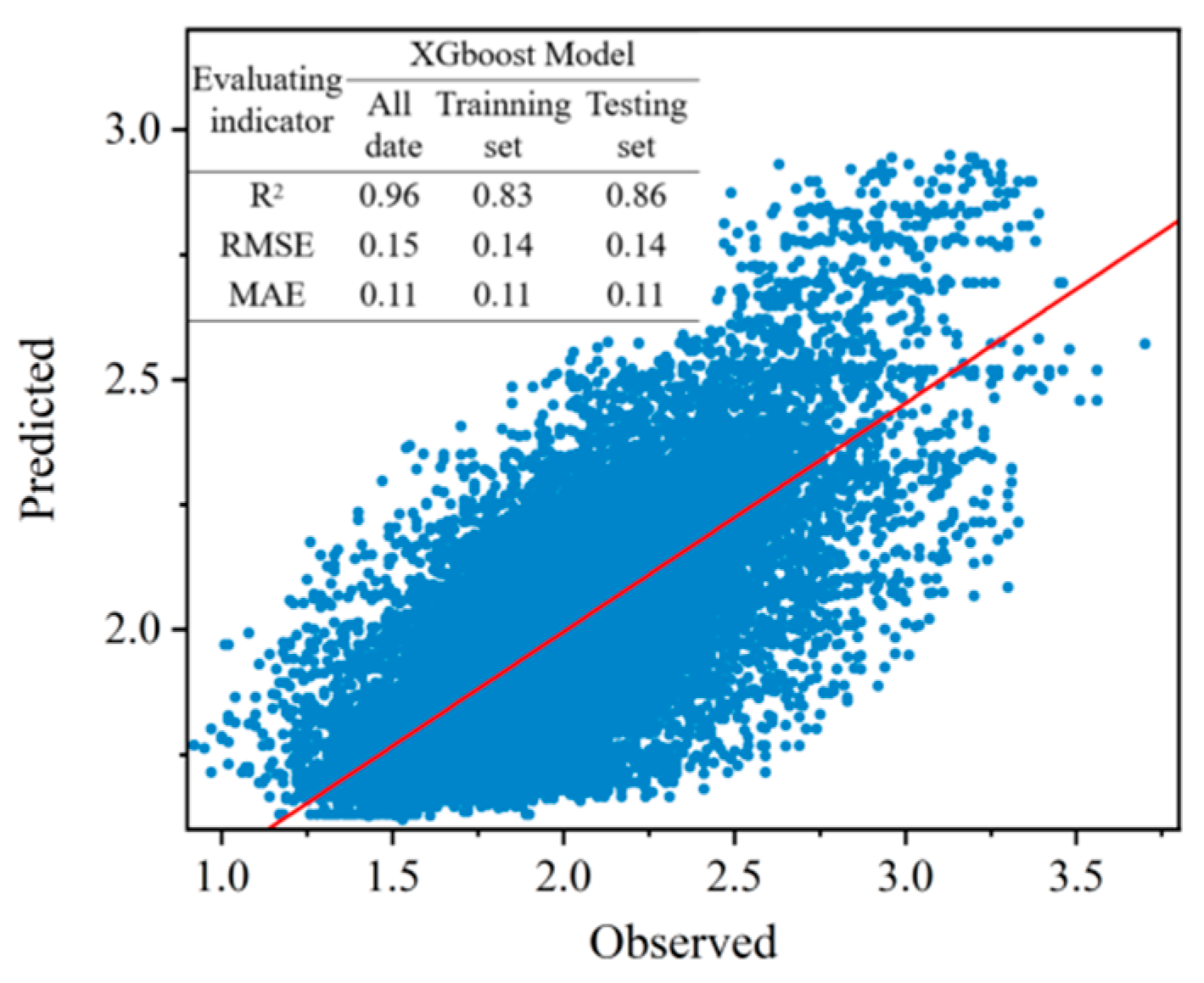
An XGBoost machine learning model was developed using Python (version 3.1.2); 80% of the data were used for training, and 20% for testing. Spatial 10-fold cross-validation was used to tune the model parameters. The final full-sample MAE was 0.11, RMSE was 0.15, and R2 was 0.96. The key parameters were set as follows: 60 decision trees, a tree depth of 5, and a learning rate of 0.03. The evaluation results are shown in Figure 2.
SHAP is an additive feature attribution method based on the Shapley value principle from game theory, commonly used to explain complex models. It quantifies the importance of each influencing factor and converts it into the corresponding SHAP value [54]. The formula for calculating the SHAP value is as follows:
S H A P ( f , x , S ) = T S T ! ( n T ) ! n ! f ( x ) f ( x S / T )
S H A P ( f , x , S / i ) = f ( x ) S H A P ( f , x , S )
where f is the predictive function of the model; x is the observed feature vector; S is the set of all features; n is the number of features; and xs/t is the observed values of all features except T.
(7)
Analysis of Dominant Factors
The factor importance index (fi) is defined as the mean of the absolute SHAP values for each factor across all valid locations within the study area. This index quantifies the aggregate influence of each factor on the variation in WUEc. The equation is as follows:
f i = m e a n k ( 1 , 2 , , n ) ( S H A P i , k ( f , x , S ) )
where i denotes the ith influencing factor and n denotes the number of all valid samples in the study area.
The primary driver ( p r i m ) is defined as the influencing factor with the largest absolute SHAP value among all influencing factors at each point within the study area. The equation is as follows:
p r i m = max i 1 , 2 , , M ( S H A P i ( f , x , S ) )
where M is the number of input features for a single sample.

3. Results

3.1. Characterization of Spatial and Temporal Variations of WUEc

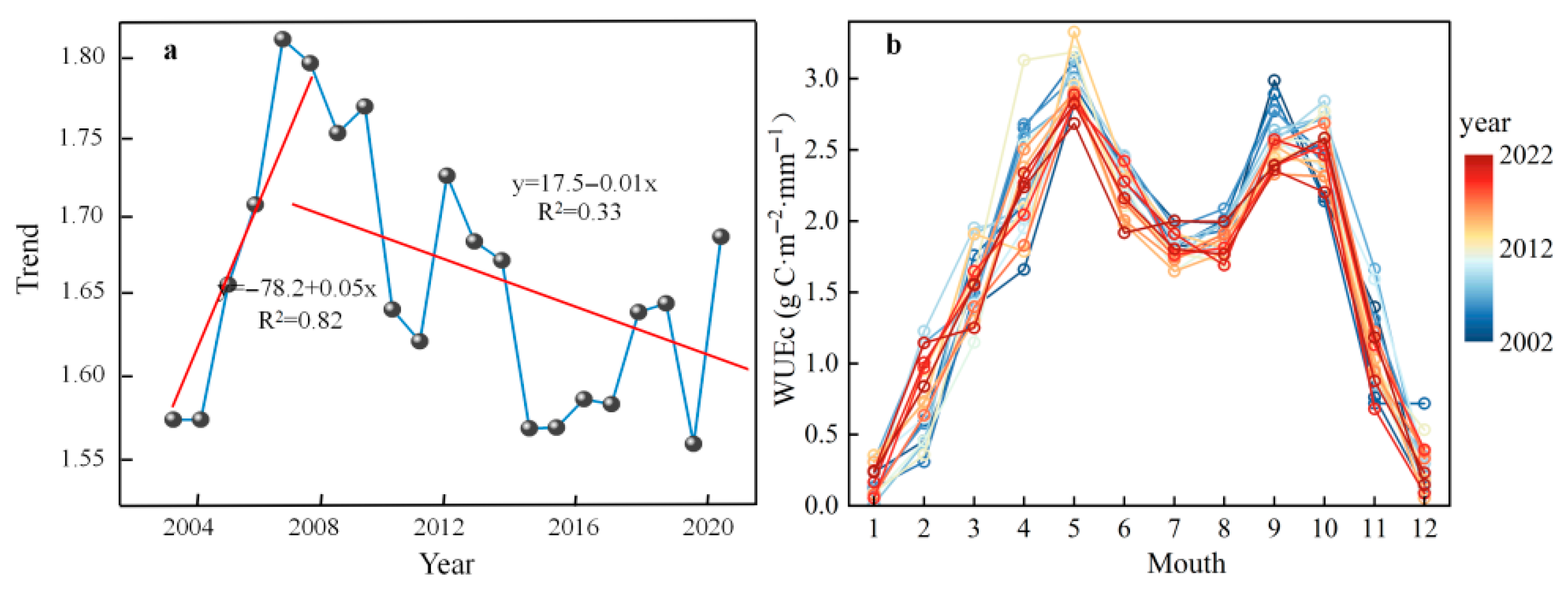
Analyzing the interannual trend, Xinjiang’s WUEc showed an increasing trend from 2002 to 2007, followed by a decreasing trend from 2008 to 2022 (Figure 3a). From 2002 to 2007, Xinjiang’s WUEc increased by an average of 0.05 gC·mm−1·m−2 per year, with a total increase of 0.3 gC·mm−1·m−2. From 2008 to 2022, Xinjiang’s WUEc decreased by an average of 0.01 gC·mm−1·m−2 per year, with a total decrease of 0.15 gC·mm−1·m−2.
Intra-annual variation analysis shows that Xinjiang’s WUEc exhibits a distinct bimodal pattern, with peaks in May and September or October (multiyear mean values consistently exceeding 2.5 gC·mm−1·m−2). Xinjiang’s WUEc was lower in winter and early spring, generally below 0.5 gC·mm−1·m−2. Over time, Xinjiang’s WUEc not only showed an overall decrease during the growing season (April–October), but also saw the maximum WUEc shift from September to October (Figure 3b).
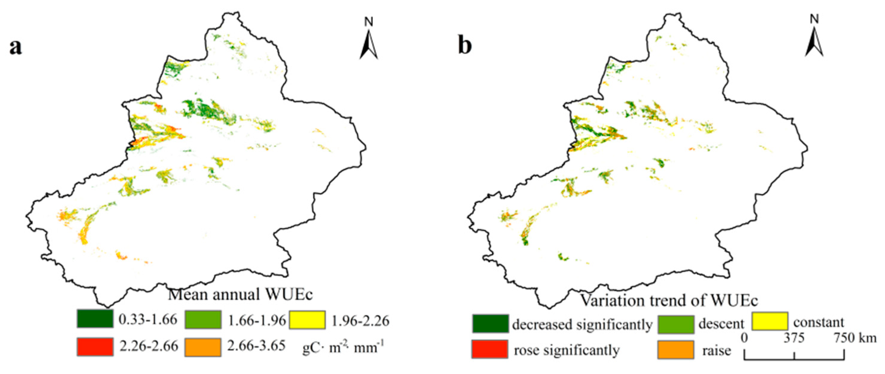
The average WUEc value in Xinjiang from 2002 to 2022 was 2.02 gC·mm−1·m−2, exhibiting an overall distribution pattern with higher values in the southwest and lower values in the northeast (Figure 4a). Specifically, Kashi and Hetian have higher WUEc (with values concentrated between 1.96 and 2.26 gC·mm−1·m−2), while Changji and Karamay have lower WUEc (with values concentrated between 0.33 and 1.66 gC·mm−1·m−2). The overall WUEc in Xinjiang exhibited a decreasing trend. Specifically, 52.26% of the region showed a decreasing trend, covering most of the study area. A significant decreasing trend was observed in 20.81% of the region, mainly in the northern part of Yili and Kelamayi. In contrast, 19.86% of the region exhibited an increasing trend, mainly in the southern part of Aksu, Yili Prefecture, and Kashi. Only 3.7% of the region showed a significant increasing trend in WUEc, primarily in Kashi (Figure 4b). The overall trend of WUEc in Xinjiang from 2002 to 2022 was a decrease, indicating a decline in the efficiency of the carbon and water cycle in cropland during this period.

3.2. Sustainability and Stability Analysis of WUEc

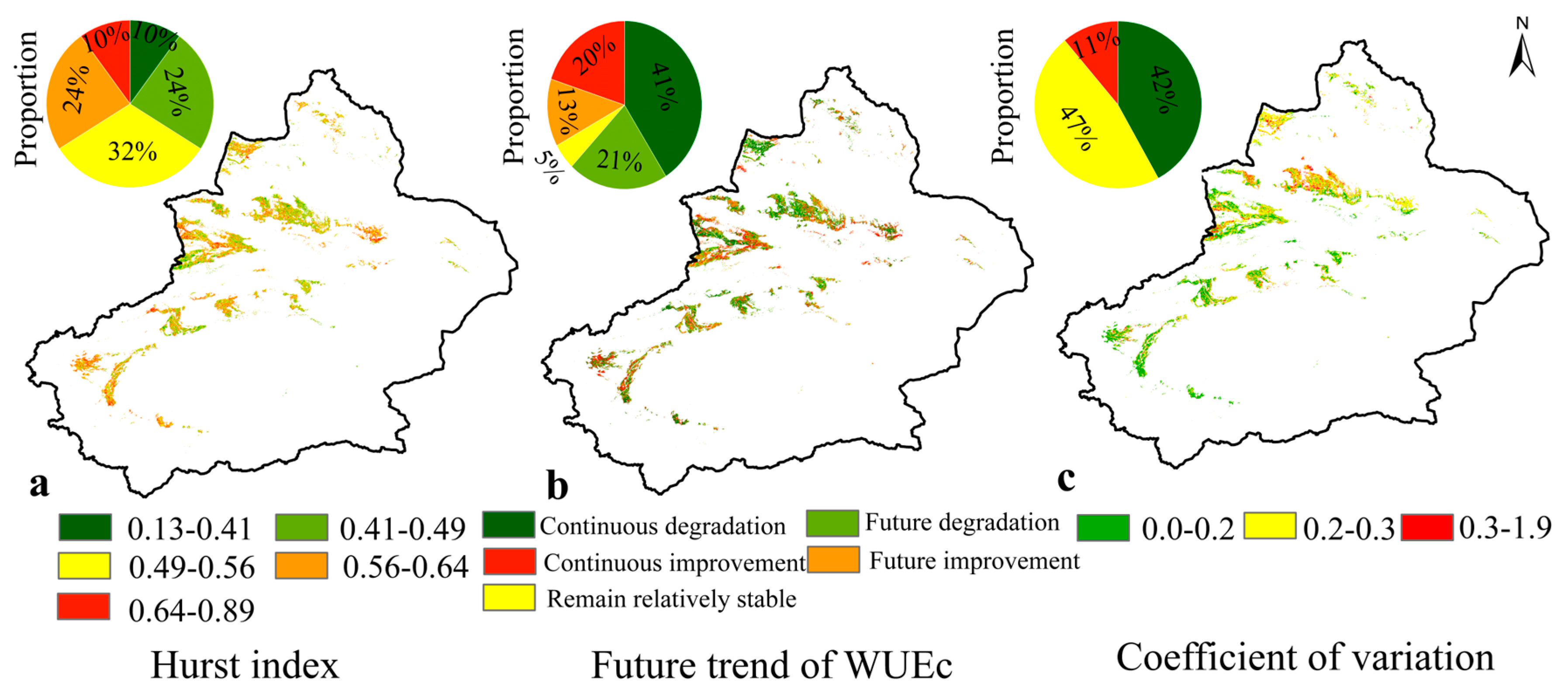
From 2002 to 2022, the Hurst index of WUEc in Xinjiang fluctuated between 0.13 and 0.89, with a mean value of 0.52. Of these, regions with a Hurst index greater than 0.5 accounted for 71% of the study area and were predominantly characterized by anti-persistence (Figure 5a). To further analyze the future trend of WUEc in Xinjiang, the results from the Mann–Kendall trend analysis were combined with the Hurst analysis outcomes to forecast future WUEc changes, with all change categories being mutually exclusive. In the future, Xinjiang’s WUEc is predominantly characterized by a decreasing trend (62.4% of the region). Within this, areas experiencing a persistent decline account for 41.1% of the study area, primarily located in Karamay and Tacheng; regions expected to experience future decline account for 21.3%, primarily in Aksu, Bazhou, and central Yili; regions with an increasing trend are concentrated in Yili and Changji, making up 32.3% of the region. Meanwhile, regions with a stable and unchanging trend account for only 5.3% of the region (Figure 5b). The mean CV of WUEc in Xinjiang is 0.23, indicating low variability and high stability. In terms of distribution, the CV gradually increases from north to south. Specifically, 41.9% of the CV values fall within the range of 0 to 0.2, primarily concentrated in the southern part of the study area (e.g., Aksu, Hetian, and Tacheng). Meanwhile, 46.9% fall within the range of 0.2 to 0.3, mostly in central Yili, Changji, and northern Tacheng. Only 11.2% of the areas have higher CV values (ranging from 0.3 to 1.9), mainly located in the central part of the study area, where human activities are more frequent, such as in Urumqi, Turpan, and Karamay (Figure 5c).

3.3. Attribution Analysis of WUEc Changes in Xinjiang

3.3.1. The Response of WUEc Variation to Climate and Vegetation Factors

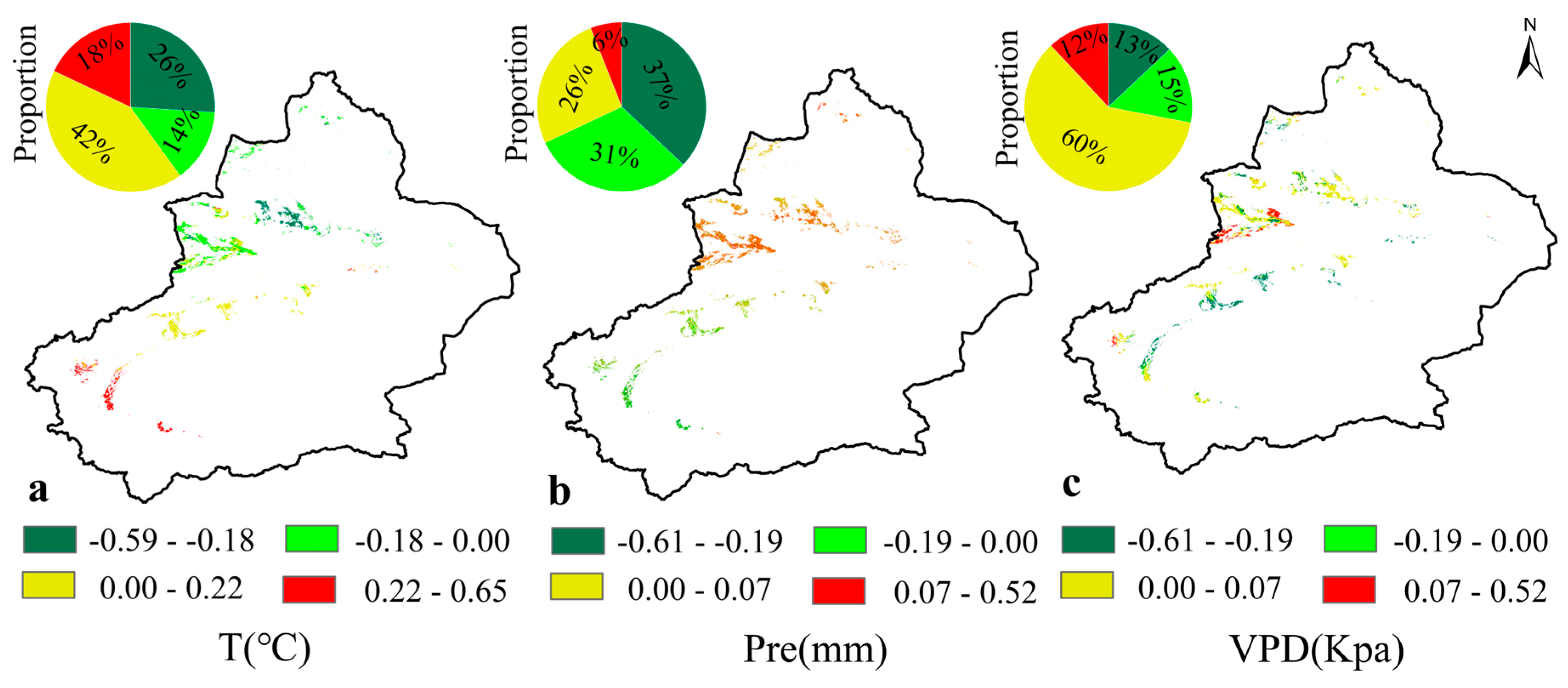
The overall negative correlation between T and WUEc in Xinjiang is observed in 60% of the region, with the spatial distribution of SHAP values showing a decreasing trend from south to north (Figure 6a). Kashi and Kezhou have higher SHAP values, ranging from 0.22 to 0.65 gC·mm−1·m−2, covering 26% of the region. Urumqi and Changji, on the other hand, exhibit lower SHAP values, ranging from −0.59 to −0.18 gC·mm−1·m−2, covering 18% of the region. Pre showed a positive correlation with WUEc in Xinjiang overall (68% of positively correlated regions), and the SHAP values displayed a spatial upward trend from south to north, which contrasts with the spatial distribution of SHAP values for T and WUEc (Figure 6b). In Kashi and Hetian, Pre was negatively correlated with WUEc, with SHAP values ranging from −0.61 to −0.19 gC·mm−1·m−2, accounting for 18% of the region. The higher SHAP values for Pre and WUEc were concentrated in northern Yili and Bozhou, with SHAP values ranging from 0.07 to 0.52 gC·mm−1·m−2, covering 37% of the region. The SHAP values for VPD and WUEc were more evenly distributed and showed weak correlation overall in the study area. Sixty percent of the area exhibited smaller SHAP values (−0.15 to 0.00 gC·mm−1·m−2), while the areas with higher SHAP values were mainly concentrated in Yili (Figure 6c).
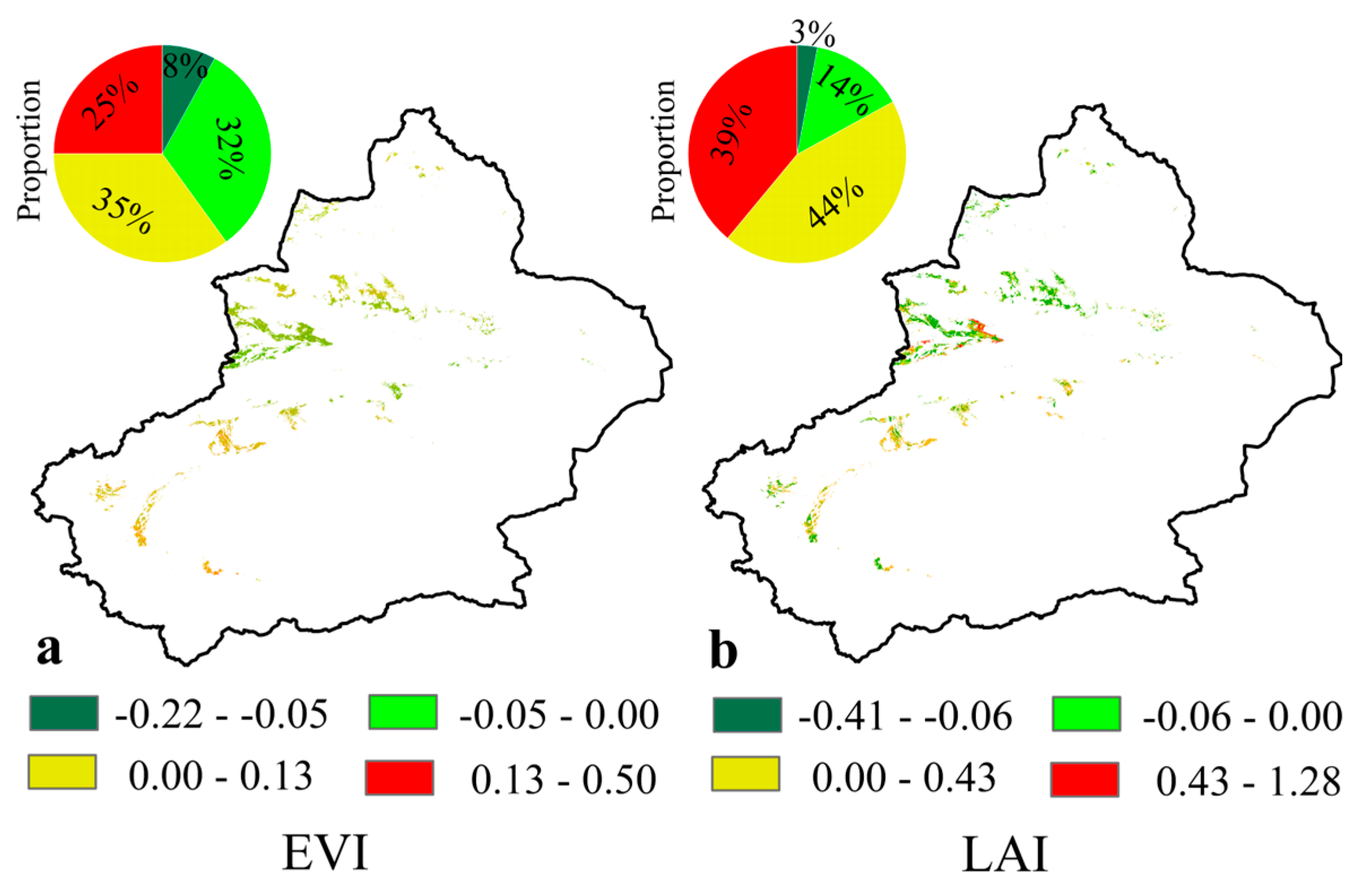
The correlation between EVI and WUEc in Xinjiang was weak, whereas LAI exhibited a relatively strong negative correlation with WUEc. Specifically, the SHAP values of EVI and WUEc are relatively evenly distributed across the study area, with generally smaller values. Areas with SHAP values ranging from −0.05 to 0.13 gC·mm−1·m−2 account for 67% of the region. The SHAP values for LAI and WUEc exhibit a decreasing trend from south to north. The areas with lower SHAP values (−0.42 to −0.06 gC·mm−1·m−2) are mainly concentrated in Bozhou, Changji, and most parts of Yili, accounting for 39% of the region. Meanwhile, areas with higher SHAP values (0.43 to 1.28 gC·mm−1·m−2) account for only 3% and are primarily located in a small portion of the eastern part of Yili (Figure 7).

3.3.2. Analysis of Dominant Factors in WUEc Changes

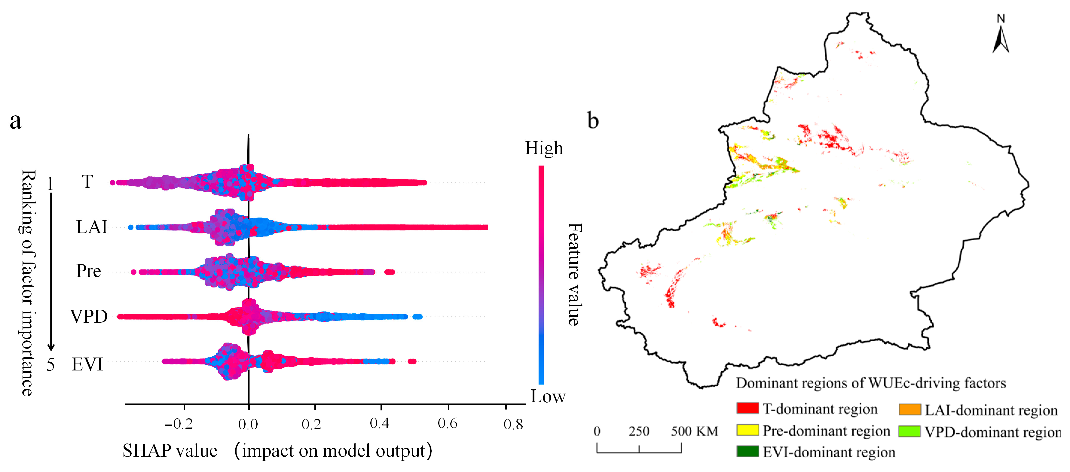
Based on the SHAP values of meteorological and vegetation factors influencing WUEc in Xinjiang, we created a ranked map showing each factor’s contribution to WUEc and a spatial distribution map of its dominant regions (Figure 8). The importance index and the percentage of each factor’s dominant region are also summarized in Table 2. The results show that T is the primary factor influencing the change in WUEc in Xinjiang, with an importance index of 0.15 gC·mm−1·m−2, much higher than that of the other influencing factors. T is the dominant factor driving changes in WUEc across 45.7% of the study area, primarily concentrated in Hetian, Aksu, Changji, Urumqi, and Kelamayi. LAI ranks second in the importance of all influencing factors, with an importance index of 0.1 gC·mm−1·m−2 for WUEc in Xinjiang. Its dominant influencing area is concentrated in the northern regions of Aksu and Yili, covering 17.6% of the study area. The importance index of Pre on WUEc in Xinjiang is 0.09 gC·mm−1·m−2, with its dominant area accounting for 17.4% of the study area, primarily in the southern part of Aksu and the northern part of Yili. The importance index of VPD was slightly smaller than that of precipitation, at 0.08 gC·mm−1·m−2. It is the dominant factor driving changes in WUEc across 14.7% of the study area, mainly concentrated in the southern region of Yili. The effect of EVI on WUEc in Xinjiang was not significant, with an importance index of 0.05 gC·mm−1·m−2. It was the dominant factor driving changes in WUEc in only 4.3% of the cropland areas in Xinjiang.

3.4. Nonlinear Relationships and Effective Thresholds of Influencing Factors on WUEc

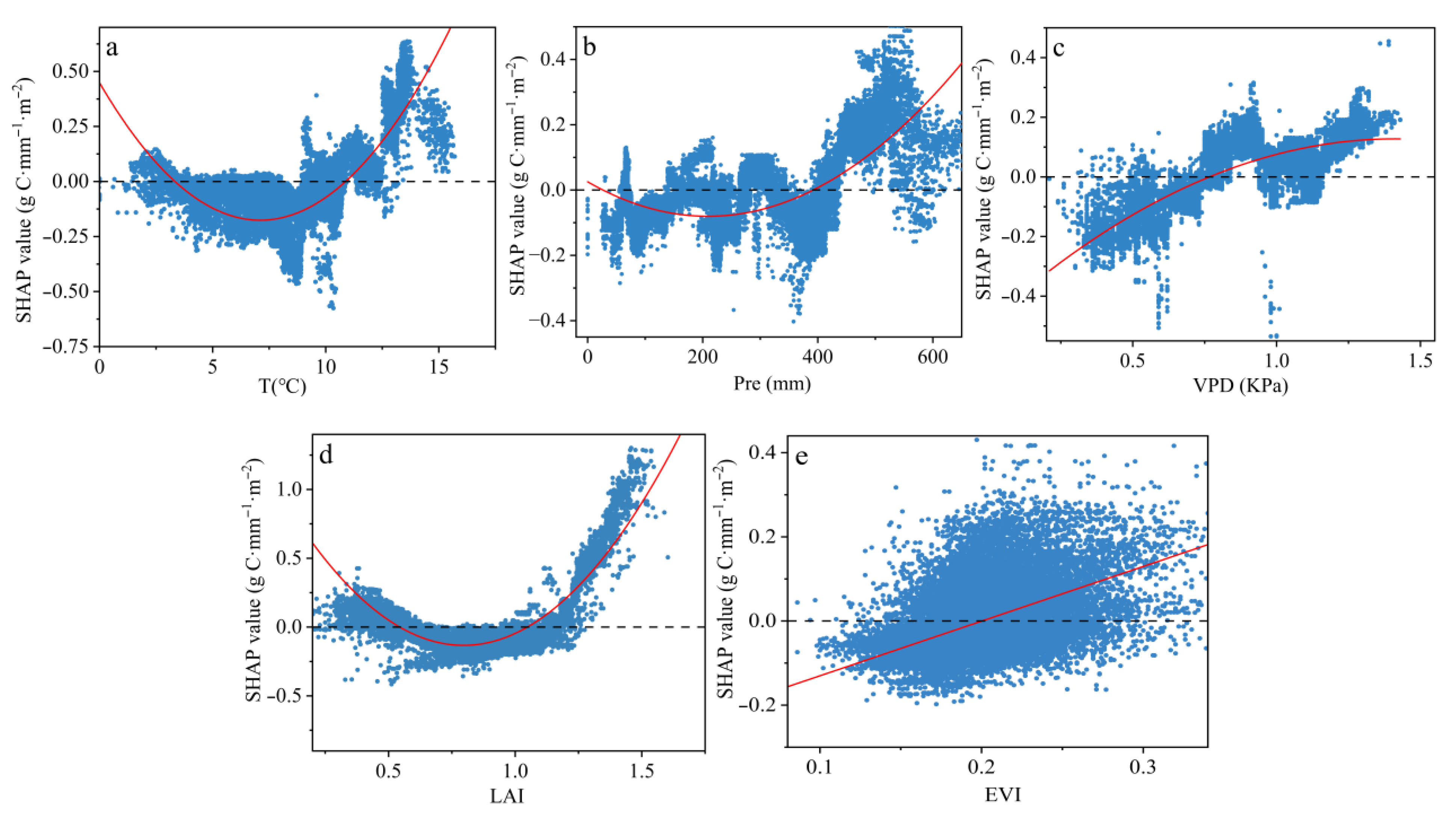
Although the previous section identified the primary drivers of WUEc, understanding their nonlinear responses is crucial for accurately predicting how WUEc will behave under varying conditions. To quantify the contribution patterns of each driver, we created dependence scatter plots (Figure 9).
Overall, temperature, VPD, and LAI are negatively correlated with WUEc, while precipitation is positively correlated with it. Each of these relationships exhibits distinct thresholds. No clear correlation is found between EVI and WUEc. Specifically, when the temperature is below 8 °C, WUEc shows a negative correlation with temperature. Between 8 °C and 14 °C, the SHAP values for temperature increase steadily, resulting in a rise in WUEc with increasing temperature. Once the temperature exceeds 14 °C, the rate of WUEc increase begins to slow (Figure 9a). For precipitation, when rainfall is below 300 mm, WUEc increases with increasing rainfall. Between 300 mm and 400 mm, WUEc generally declines. When rainfall exceeds 400 mm, the positive correlation between WUEc and precipitation becomes significantly stronger (Figure 9b). A clear threshold for VPD appears at 0.75 kPa: below this value, WUEc is negatively correlated with VPD, whereas above it, the correlation becomes positive. LAI exhibits thresholds at approximately 0.5 and 1.25 (Figure 9c). When LAI is below 0.5 or above 1.25, it is primarily positively correlated with WUEc. Within the range of 0.5 to 1.25, WUEc tends to decline as LAI increases (Figure 9d). For EVI, the positive and negative SHAP values are nearly balanced across Xinjiang, indicating no significant correlation with WUEc (Figure 9e).

4. Discussion

4.1. Attribution Analysis of the Spatiotemporal Variations in WUEc in Xinjiang

This study demonstrates that crop water-use efficiency (WUEc) in Xinjiang exhibited an overall declining trend from 2002 to 2022, with a marked inflection point in 2007—rising before 2007 and decreasing thereafter. This pattern is consistent with previous findings; however, the underlying causes remain under debate. For example, Gao et al. [55] applied the CASA model to estimate NPP and actual ET, and analyzed the spatiotemporal variations in WUE across Xinjiang from 1990 to 2020, identifying key driving forces of WUE changes. Their results indicate that precipitation and evapotranspiration were the primary contributors to the decline in WUE across the region. In contrast, Yahefujiang et al. utilized MODIS data to explore the dominant factors influencing WUE in Central Asia (including Xinjiang) from 2001 to 2020, and found that interannual variation in WUE was mainly driven by GPP, with WUE dynamics closely mirroring those of GPP [56]. Considering the climatic changes and agricultural policy shifts in Xinjiang during 2002–2022, these discrepancies may be attributed to the following reasons: before 2007, a warmer and wetter climate, combined with policies such as the “grain-to-cotton” transition and land consolidation, led to a 35% increase in cotton planting area in southern Xinjiang, thereby enhancing WUEc. After 2007, rising temperatures, decreasing precipitation, expansion of low-productivity saline–alkali lands, and diminished water availability jointly contributed to a sharp decline in WUEc [57,58].
The conclusions of existing studies regarding the spatial differences in WUE between southern and northern Xinjiang remain inconsistent. For instance, Gao et al. calculated WUE in Xinjiang from 1990 to 2020 using MODIS data and found that WUE in the southern plains was higher than in the mountainous areas of northern Xinjiang [55]. In contrast, Song et al. employed a fuzzy comprehensive evaluation model and reported that the average WUE in northern Xinjiang (e.g., Urumqi, Karamay) was 3.32 gC·m−2, which was higher than the 2.39 gC·m−2 observed in southern regions such as Aksu and Kashgar [59]. This discrepancy may stem from the different data sources used in WUE estimation. The conclusions of the present study are consistent with those of Gao, and the observed differences may primarily result from variations in regional climate conditions and cropping structures. Southern Xinjiang is rich in thermal and solar resources and benefits from glacial meltwater and well-developed irrigation infrastructure, which ensures a stable water supply and, thus, enhances WUEc. In contrast, although northern Xinjiang receives slightly more precipitation, it experiences lower temperatures and shorter growing seasons, with WUEc being constrained by thermal limitations [60]. Therefore, we recommend adopting region-specific strategies to implement the “water and land red line” policy, which includes reducing low-yield, inefficient farmland in northern Xinjiang and steadily improving agricultural productivity in the south, thereby enhancing the overall WUEc level across the region.

4.2. The Impact of Meteorological Factors on WUEc Variation

Xue et al. analyzed global patterns and drivers of WUE from 2000 to 2013 using MODIS data and identified a negative correlation between WUE and temperature [61], while Zhou et al. reported a positive relationship [62]. In this study, we found that WUEc in Xinjiang during 2002–2022 was generally negatively correlated with temperature; however, about 40% of the region exhibited a positive relationship. This pattern may result from a pronounced threshold effect of temperature on WUEc: at lower temperatures, the activity of photosynthetic enzymes is suppressed, reducing GPPc synthesis; at higher temperatures, stomatal closure limits CO2 uptake, thereby constraining GPPc production and ultimately decreasing WUEc [63,64]. In the study area, the negative effect of temperature is primarily attributed to an increased diurnal temperature range during the growing season, wherein elevated transpiration surpasses the improvement in leaf carbon assimilation. This finding aligns with previous studies on temperature threshold effects [65]. The influence of precipitation on WUE remains contentious. For example, Bai et al. [66] identified a positive correlation between WUE and precipitation using eddy covariance tower measurements, whereas Sun [67], employing a process-based model, observed a negative correlation. Sun et al. [67] attributed this discrepancy to methodological differences between site-level observations and spatially integrated regional estimates. However, in arid regions, the influence of precipitation on WUE tends to be more consistent. For instance, Liu et al. [68] found that in regions with annual precipitation below 500 mm, vegetation in most terrestrial ecosystems across China exhibited a positive WUE response. Similarly, Li [26] reported that more than 60% of the desert steppe in Inner Mongolia exhibited a positive spatial correlation between WUE and precipitation, consistent with the findings of this study. This consistency may result from the extremely low mean annual precipitation in the study area—less than 160 mm, far below the 500 mm threshold—leading to a positive response of WUEc to increased precipitation. It is generally accepted that WUE declines with increasing vapor pressure deficit (VPD) [32]. However, studies by Eamus and Reichstein et al. [69,70] suggest that WUE’s negative response to VPD may only occur during specific seasons, or may even be absent under extreme environmental conditions. In the arid and semi-arid regions under study, irrigation is widely employed to sustain crop growth. For irrigated crops, transpiration rates are inversely related to atmospheric humidity, which is often represented by VPD. Therefore, WUEc generally exhibits a negative correlation with VPD under such conditions.

4.3. The Impact of Vegetation Factors on WUEc Dynamics

As an essential indicator of vegetation growth, the LA affects both plant development and the allocation of evapotranspiration between transpiration and evaporation. Consequently, it plays a key regulatory role in GPP and actual ET, ultimately influencing WUEc [68,71]. However, the effect of LAI on WUEc via its influence on the GPPc/ETc ratio remains debated. For instance, Chu et al. and Luo et al. reached opposing conclusions based on remote sensing data: Chu et al. reported that increased LAI elevated ET, thereby decreasing WUE [72], while Luo et al. found that LAI significantly enhanced GPP, leading to improved WUE [73]. In this study, approximately 83% of the region exhibited a negative correlation between LAI and WUEc. This trend may result from changes in cropping structure, which have led to increased LAI and higher agricultural water consumption. Strong evaporative demand and the continued use of traditional surface irrigation in the study area have exacerbated leaf water loss, limiting the ability of photosynthesis to offset the increase in ETc and ultimately reducing WUEc. In contrast, the correlation between the EVI and WUEc was relatively weak, aligning with the findings of Tian et al. in arid regions [25]. However, some studies have reported a positive influence of EVI on WUEc. For instance, Tang et al. [74] integrated eddy covariance tower data with MODIS-derived EVI to investigate WUEc drivers and found a significant positive correlation. The divergence between their findings and ours may stem from the dual role of EVI. On the one hand, higher EVI enhances vegetation cover and photosynthetic capacity, potentially boosting GPPc and improving WUEc. On the other hand, increased transpiration leads to greater water loss, which may offset these gains. This trade-off likely accounts for the weak overall correlation between EVI and WUEc observed in this study [75,76].

4.4. Potential Applications and Limitations

This study comprehensively examined various climatic and vegetation factors and employed multiple trend detection and factor attribution methods to analyze WUEc trends in Xinjiang from 2002 to 2022 and identify key drivers. However, several uncertainties remain. Although WUEc is defined as the ratio of GPPc to ETc, this definition neglects additional water-consuming processes relevant to agricultural production, including runoff, surface evaporation, and deep percolation. MODIS-based WUE estimates are generally reliable—validated using flux-tower data with R2 values ranging from 0.74 to 0.963—but systematic biases of 10–20% remain, particularly in drip-irrigated cotton fields under mulch [77]. While this study emphasized major climatic (temperature, precipitation, VPD) and vegetation (LAI, EVI) drivers, WUEc is also affected by stomatal conductance, phenology, drought stress, and CO2 fertilization. Future research should incorporate direct monitoring of hydrological losses and expand flux-tower networks in drylands to enhance model calibration. Additionally, further exploration of factors influencing WUEc is essential to support the sustainable development of agricultural ecosystems in arid regions.

5. Conclusions

Quantitatively assessing the spatiotemporal variation of WUEc and its primary driving factors is crucial for understanding the impact of environmental changes on the carbon balance of agricultural ecosystems. This study employed remote sensing data and geographic information system (GIS) techniques to analyze the spatiotemporal variation and major drivers of WUEc in Xinjiang from 2002 to 2022. The results reveal an overall decline in WUEc, accompanied by marked spatial heterogeneity between southern and northern Xinjiang. Excessive evaporative loss, which leads to persistently low WUEc levels, constitutes a major constraint on agricultural development in the region. To address this issue, we recommend the implementation of soil and water conservation measures—such as building irrigation infrastructure and establishing windbreaks—and the promotion of advanced irrigation techniques, including subsurface drip and infiltration irrigation, to reduce water loss and enhance WUEc. The findings also offer critical insights and a scientific foundation for future research on carbon–water interactions, as well as for regional water resource management and land-use planning in Xinjiang.

Author Contributions

Author contributions: Q.Z., conceptualization, formal analysis, investigation, methodology, supervision, visualization, writing—original draft; F.G., investigation, writing—original draft, data curation, and formal analysis; B.H., methodology, and visualization; H.L., Y.L., methodology; Y.X., R.L., investigation. All authors have read and agreed to the published version of the manuscript.

Funding

This study was supported by the 2024 research project of “Xinjiang Key Laboratory of Hydraulic Engineering Safety and Water Disaster Prevention and Control” (ZDSYS-YJS-2024-24), the Xinjiang Uygur Autonomous Region Major Scientific and Technological Special Project—Research and Demonstration on the Development Model of Ecological Agriculture and Efficient Utilization of Soil and Water Resources in Modern Irrigation Areas (2023A02002-1).

Data Availability Statement

The original contributions presented in this study are included in the article; further inquiries can be directed to the corresponding author.

Conflicts of Interest

The authors declare that the research was conducted in the absence of any commercial or financial relationships that could be construed as potential conflicts of interest.

References

  1. Scheierling, S.M.; Tréguer, D.O. Beyond Crop per Drop: Assessing Agricultural Water Productivity and Efficiency in a Maturing Water Economy; World Bank: Washington, DC, USA, 2018. [Google Scholar]
  2. Zhang, P.; Long, A.H.; Hai, Y.; Deng, X.Y.; Wang, H.; Liu, J.; Li, Y. Spatiotemporal variations and driving forces of agricultural water consumption in Xinjiang during 1988–2015: Based on statistical analysis of crop water footprint. J. Glaciol. Geocryol. 2021, 43, 242–253. [Google Scholar] [CrossRef]
  3. Cao, R.C.; Hu, Z.G.; Jiang, Z.Y.; Yang, Y.T.; Zhao, W.; Wu, G.; Feng, X.M.; Chen, R.R.; Hao, G.G. Shifts in ecosystem water use efficiency on China’s Loess Plateau caused by the interaction of climatic and biotic factors over 1985–2015. Agric. For. Meteorol. 2020, 291, 108100. [Google Scholar] [CrossRef]
  4. Farquhar, G.D.; Schulze, E.D.; Kuppers, M. Responses to humidity by stomata of Nicotiana-glauca l and Corylus-avellanal are consistent with the optimization of carbon-dioxide uptake with respect to water-loss. Aust. J. Plant Physiol. 1980, 7, 315–327. [Google Scholar] [CrossRef]
  5. Liu, C.; Liu, B.; Zhao, W.Z.; Zhu, Z.C. Temporal and spatial variability of water use efficiency of vegetation and its response to precipitation and temperature in Heihe River Basin. Acta Ecol. Sin. 2020, 40, 888–899. [Google Scholar] [CrossRef]
  6. Hatfield, J.L.; Dold, C. Water-use efficiency: Advances and challenges in a changing climate. J. Front. Plant Sci. 2019, 10, 103. [Google Scholar] [CrossRef]
  7. Du, X.Z.; Zhao, X.; Zhou, T.; Jiang, B.; Xu, P.P.; Wu, D.H.; Tang, B.J. Effects of climate factors and human activities on the ecosystem water use efficiency throughout northern China. Remote Sens. 2019, 11, 2766. [Google Scholar] [CrossRef]
  8. Dong, Y.L.; Li, Y.B.; Ma, Y.Z.; Wan, S.M.; Dong, H.Q.; Yang, B.F.; Feng, L.; Gao, F.; Zhou, J.; Wang, C. Response of soil moisture spatiotemporal variations and utilization efficiency to planting density in cotton fields in arid regions. Agric. Res. Arid Areas 2025, 1, 168–179. [Google Scholar] [CrossRef]
  9. Huang, M.T.; Zhai, P.M.; Piao, S.L. Divergent responses of ecosystem water use efficiency to drought timing over Northern Eurasia. Environ. Res. Lett. 2021, 16, 045016. [Google Scholar] [CrossRef]
  10. Mu, Y.M.; Jia, X.; Ye, Z.Q.; Guo, X.L.; Hao, S.R.; Zhao, T.S.; Zhang, Y.Q.; Han, C.; Gao, S.; Xing, F.; et al. Vegetation factors and atmospheric dryness regulate the dynamics of ecosystem water use efficiency in a temperate semiarid shrubland. J. Hydrol. 2024, 639, 131644. [Google Scholar] [CrossRef]
  11. Aaron, H.; Gabriela, P.Q.; Hannah, D. The development and current challenges of irrigated agriculture in the western U.S. Agric. Water Manag. 2025, 315, 0378–3774. [Google Scholar] [CrossRef]
  12. Lin, S.; Wang, G.X.; Hu, Z.Y.; Sun, X.Y.; Song, C.L.; Huang, K.W.; Sun, J.; Yang, Y. Contrasting response of growing season water use efficiency to precipitation changes between alpine meadows and alpine steppes over the Tibetan Plateau. Agric. Water Manag. 2023, 289, 108571. [Google Scholar] [CrossRef]
  13. Wang, F.; Wang, Z.; Huang, J.; Yang, S.J.; He, G.J.; Zhang, Y. Spatio-temporal distribution characteristics of cropland water use efficiency and its relationship with climate in Anhui Province. Acta Ecol. Sin. 2019, 38, 6268–6279. [Google Scholar] [CrossRef]
  14. Chang, M.; Shi, H.G.; Yuan, S.Y.; Chen, K.L.; Zhang, X.Y.; Zhang, J.H. How does farmer differentiation effect agricultural water use efficiency? Evidence from China. Agric. Water Manag. 2025, 312, 0378–3774. [Google Scholar] [CrossRef]
  15. Nie, C.; Huang, Y.F.; Zhang, S.; Yang, Y.T.; Zhou, S.; Lin, C.J.; Wang, G.Q. Effects of soil water content on forest ecosystem water use efficiency through changes in transpiration/evapotranspiration ratio. Agric. For. Meteorol. 2021, 308, 108605. [Google Scholar] [CrossRef]
  16. Térán, C.P.; Naz, B.S.; Graf, A.; Qu, Y.Q.; Franssen, H.-J.H.; Baatz, R.; Clais, P.; Vereecken, H. Rising water-use efficiency in European grasslands is driven by increased primary production. Commun. Earth Environ. 2023, 4, 95. [Google Scholar] [CrossRef]
  17. Shang, B.; Agathokleous, E.; Calatayud, V.; Peng, J.; Xu, Y.; Li, S.; Liu, S.; Feng, Z. Drought mitigates the adverse effects of O3 on plant photosynthesis rather than growth: A global meta-analysis considering plant functional types. Plant Cell Environ. 2024, 47, 1269–1284. [Google Scholar] [CrossRef]
  18. Guo, L.M.; Shan, N.; Zhang, Y.G.; Sun, F.B.; Liu, W.B.; Shi, Z.J.; Zhang, Q. Separating the effects of climate change and human activity on water use efficiency over the Beijing-Tianjin Sand Source Region of China. Sci. Total Environ. 2019, 690, 584–595. [Google Scholar] [CrossRef]
  19. Tian, F.; Yang, J.H.; Du, R.H.; Lin, J.H.; Chen, M.; Wu, J.J. Sustained vegetation greening enhanced ecosystem water-use efficiency in the Loess Plateau of China in recent 20 years. Ecol. Eng. 2022, 184, 106768. [Google Scholar] [CrossRef]
  20. Wang, L.M.; Li, M.Y.; Wang, J.X.; Li, X.G.; Wang, L.C. An analytical reductionist framework to separate the effects of climate change and human activities on variation in water use efficiency. Sci. Total Environ. 2020, 727, 138306. [Google Scholar] [CrossRef]
  21. Wang, Y.; Tong, X.; Li, J.; Yang, M.; Wang, Y. Impacts of Climate Change and Human Activities on Vegetation Productivity in China. Remote Sens. 2025, 17, 1724. [Google Scholar] [CrossRef]
  22. Sun, H.; Fang, G.F.; Ruan, L.L.; Li, S.N.; Zhang, L. Spatiotemporal Patterns and Drivers of Carbon and Water Fluxes in Semi-Arid Regions of Asia. Acta Ecol. Sin. 2022, 42, 4742–4757. [Google Scholar] [CrossRef]
  23. Hu, Z.Y.; Dai, Q.H.; Yan, Y.J.; Zhang, Y.; Li, H.Y.; Zhou, H. Dissecting the characteristics and driver factors on global water use efficiency using GLASS data sets. Earth’s Future 2024, 12, e2024EF004630. [Google Scholar] [CrossRef]
  24. Yu, H.C.; Li, S.E.; Ding, J.; Yang, T.Y.; Wang, Y.X. Water use efficiency and its drivers of two typical cash crops in an arid area of Northwest China. Agric. Water Manag. 2023, 287, 108433. [Google Scholar] [CrossRef]
  25. Tian, F.; Zhang, Y.; Lu, S. Spatial-temporal dynamics of cropland ecosystem water-use efficiency and the responses to agricultural water management in the Shiyang River Basin, northwestern China. Agric. Water Manag. 2020, 237, 106176. [Google Scholar] [CrossRef]
  26. Li, H.; Liu, T.J.; Wang, S.H.; Liu, D.W. Spatial and temporal variation of water use efficiency and its influencing factors in desert steppe of Inner Mongolia from 2001 to 2021. Arid. Land Geogr. 2023, 47, 993–1003. [Google Scholar] [CrossRef]
  27. Li, Y.L.; Wu, X.Q.; Yuan, Y.; Dong, L.B. Spatial-temporal evolution and driving mechanism of vegetation carbon and water use efficiency in Heilongjiang Province, China. Chin. J. Appl. Ecol. 2024, 35, 3349–3358. [Google Scholar] [CrossRef]
  28. Wang, F.Y.; Xia, J.; Zou, L.; Zhang, L.P.; Li, X.Y.; Yu, J.R. Spatio-temporal heterogeneity and driving mechanism of ecosystem water use efficiency in the Loess Plateau, China. J. Hydrol. Reg. Stud. 2024, 56, 2214–5818. [Google Scholar] [CrossRef]
  29. Seka, A.M.; Zhang, J.H.; Ayele, G.T.; Demeke, Y.G.; Han, J.Q.; Prohan, F.A. Spatio-temporal analysis of water storage variation and temporal correlations in the East Africa lake basins. J. Hydrol. Reg. Stud. 2022, 41, 101094. [Google Scholar] [CrossRef]
  30. Zhao, T.L.; Liu, W.; Li, Z.; Xu, Z.; Yang, K.; Wu, D. Analyses of the evolution and influencing factors of natural runoff in China based on STL decomposition. J. Hydraul. Eng. 2025, 56, 216–226+239. [Google Scholar] [CrossRef]
  31. Li, H.D.; Guan, D.J.; Yuan, F.H.; Wang, A.Z.; Jin, C.J.; Wu, J.B. Water use efficiency and its influential factor over Horqin Meadow. Acta Ecol. Sin. 2015, 35, 478–488. [Google Scholar] [CrossRef]
  32. Li, F.; Xiao, J.F.; Chen, J.Q.; Ballantyne, A.; Li, K.J.; Li, B. Global water use efficiency saturation due to increased vapor pressure deficit. Science 2023, 381, 672–677. [Google Scholar] [CrossRef]
  33. Liu, S.H.; Xue, L.Q.; Xiao, Y.; Yang, M.J.; Liu, Y.H.; Han, Q. Dynamic process of ecosystem water use efficiency and response to drought in the Yellow River Basin, China. Sci. Total Environ. 2024, 934, 173339. [Google Scholar] [CrossRef]
  34. Gevaert, C.M. Explainable AI for earth observation: A review including societal and regulatory perspectives. Int. J. Appl. Earth Obs. Geoinf. 2022, 112, 102869. [Google Scholar]
  35. Lipton, Z.C. The mythos of model interpretability. arXiv 2016, arXiv:1606.03490. [Google Scholar]
  36. Roscher, R.; Bohn, B.; Duarte, M.F.; Garcke, J. Explain it to me-facing remote sensing challenges in the bio-and geosciences with explainable machine learning. ISPRS Ann. Photogramm. Remote Sens. Spat. Inform. Sci. 2020; V-3-2020, 817–824. [Google Scholar] [CrossRef]
  37. Sardans, J.; Miralles, A.; Tariq, A.; Zeng, F.J.; Wang, R.; Peñuelas, J. Growing aridity poses threats to global land surface. Commun. Earth Environ. 2024, 5, 776. [Google Scholar] [CrossRef]
  38. Duan, Z.R.; Jumayipu, Z.B.; Xia, J.X.; Liu, R.X. Water Consumption Characteristics and Evolution in Aksu Oasis Under Climate Variations and Land-use Changes. J. Basic Sci. Eng. 2018, 26, 1203–1216. [Google Scholar]
  39. Ni, M.X.; Muhtar, P.; Sun, T.Y.; Xia, J.X. Analysis on the Supply-demand Relationship of Water Resources Basedon the Dual Role of Climate Change and Human Activities in Southern Xinjiang, China. J. Basic Sci. Eng. 2024, 32, 331–348. [Google Scholar] [CrossRef]
  40. Zhang, C.L.; Zou, H.B.; Li, H.K.; Wang, H.Y. Tectonic framework and evolution of the Tarim Block in NW China. Gondwana Res. 2013, 23, 1306–1315. [Google Scholar] [CrossRef]
  41. Li, Y.; Dong, Y.; Zhang, Y.; Zhang, B.; Li, C. Climate Change and Human Activities Contribute to the Enhancement Recovery of Grassland Productivity in Xinjiang. Grass Forage Sci. 2024, 79, 716–733. [Google Scholar] [CrossRef]
  42. Han, C.Q.; Zheng, J.H.; Guan, D.L.; Yu, D.L. Evaluating and simulating resource and environmental carrying capacity in arid and semiarid regions: A case study of Xinjiang, China. J. Clean. Prod. 2022, 338, 130646. [Google Scholar] [CrossRef]
  43. Yang, J.; Gao, F.; Xu, H.L.; Liu, K.; Han, F.H. Spatial and Temporal Evolution of Ecosystem Service Value and Its Driving Factors in the Aksu River Basin. Environ. Sci. 2025, 46, 2385–2397. [Google Scholar]
  44. Nuermaimaiti, R.; Wang, X.M. Analysis on the Characteristics of Spatial and Temporal Changes for Land Desertification in Hotan Area, Xinjiang. J. Ecol. Rural. Environ. 2020, 36, 870–878. [Google Scholar]
  45. Cleveland, R.B.; Cleveland, W.S.; McRae, J.E. STL: A seasonal-trend decomposition procedure based on loess. J. Off. Stat. 1990, 6, 3–33. [Google Scholar]
  46. Kendall, M.G. A new measure of rank correlation. Biometrika 1938, 30, 81–93. [Google Scholar] [CrossRef]
  47. Mann, H.B. Nonparametric tests against trend. Econometrica 1945, 13, 245–259. [Google Scholar] [CrossRef]
  48. Liu, Z.Y.; Sheng, H.; Dong, Y.Y. Research on self-similarity time-varying hurst index estimation method based on weighted average method. Inf. Technol. 2019, 43, 1–4, 9. [Google Scholar]
  49. Shi, N.N.; Han, Y.; Wang, Q.; Xiao, N.W.; Quan, Z.-J. Spatial and temporal characteristics of fractional vegetation cover and its response to urbanization in Beijing. Environ. Sci. 2024, 45, 5318–5328. [Google Scholar] [CrossRef]
  50. Yuan, J.L.; Zhao, H.H.; Liu, X.H.; Li, H.Y.; Jiang, D.; Zhao, C.Y. Driving force analysis and ecological evaluation of spatiotemporal changes in vegetation cover in the Kunlun Mountains from 2000 to 2020. Geol. J. China 2024, 51, 1822–1838. [Google Scholar]
  51. Chen, T.Q.; Guestrin, C. XGBoost: A scalable tree boosting system. In Proceedings of the 22nd Acm Sigkdd International Conference on Knowledge Discovery and Data Mining, San Francisco, CA, USA, 13–17 August 2016; pp. 785–794. [Google Scholar] [CrossRef]
  52. Roscher, R.; Bohn, B.; Duarte, M.F. Explainable machine learning for scientific insights and discoveries. IEEE Access 2020, 8, 23317–23323. [Google Scholar] [CrossRef]
  53. Yan, H.B.; Liang, Y.H.; Lu, X.J.; Zhao, T.J.; Wu, S.Y.; Xu, P.J.; Zeng, J.Z. Assessing spatiotemporal dynamics of water use efficiency in ecologically vulnerable karst landscapes. J. Hydrol. Reg. Stud. 2024, 55, 2214–5818. [Google Scholar] [CrossRef]
  54. Lundberg, S.M.; Lee, S.I. A unified approach to interpreting model predictions. In Proceedings of the Neural Information Processing Systems 2017-NIPS, Long Beach, CA, USA, 4–9 December 2017. [Google Scholar]
  55. Gao, X.Y.; Hao, H.C.; Zhang, X.Q.; Chen, Y. Responses of vegetation water use efficiency to meteorological factors in arid areas of northwest China: A case of Xinjiang. Arid Land Geogr. 2023, 46, 1111–1120. [Google Scholar]
  56. Yahefujiang, H.; Zou, J.; Ding, J.; Zou, W.; Tangjialeke, W.; Yang, M. Spatial and Temporal Variation in Water Use Efficiency and Ecosystem Photosynthetic Efficiency in Central Asia. Remote Sens. 2023, 15, 5240. [Google Scholar] [CrossRef]
  57. Yao, J.Q.; Mao, W.Y.; Chen, J.; Dilinuer, T. Signal and impact of wet-to-dry shift over Xinjiang, China. Acta Geogr. Sin. 2021, 76, 57–72. [Google Scholar] [CrossRef]
  58. He, H.X.; Fu, A.H.; Wang, C. Negetation index change and its driving forces of low mountain meadow vegetation in the northwest of Tacheng Region, Xinjiang, China. J. Desert Res. 2023, 43, 187–196. [Google Scholar]
  59. Song, P.; Wang, X.; Wang, C.; Lu, M.; Chen, L.; Kong, L.; Lei, X.; Wang, H. Analysis of Agricultural Water Use Efficiency Based on Analytic Hierarchy Process and Fuzzy Comprehensive Evaluation in Xinjiang, China. Water 2020, 12, 3266. [Google Scholar] [CrossRef]
  60. Lu, J.T.; Zheng, J.H.; Peng, J.; Xiao, X.H.; Li, G.Y.; Liu, L. Spatiotemporal evolution of ecological vulnerability in Xinjiang and its response to drought. Remote Sens. Nat. Resour. 2025, 37, 253–264. [Google Scholar]
  61. Xue, B.-L.; Guo, Q.; Otto, A.; Li, L. Global patterns, trends, and drivers of water use efficiency from 2000 to 2013. Ecosphere 2015, 6, 174. [Google Scholar] [CrossRef]
  62. Zhou, J.; Zhang, Z.; Sun, G.; Fang, X.; Zha, T.; Chen, J.; Noormets, A.; Guo, J.; McNulty, S. Water-use efficiency of a poplar plantation in Northern China. J. For. Res. 2014, 19, 483–492. [Google Scholar] [CrossRef]
  63. Maimaiti, A.; Rusuli, Y.; He, H.; Abudukerimu, B. Spatio-temporal characteristics of vegetation water use efficiency and its relationship with climate factors in Tianshan Mountains in Xinjiang from 2000 to 2017. Chin. J. Plant Ecol. 2019, 44, 490–500. [Google Scholar] [CrossRef]
  64. Zhang, Y.C.; Piao, S.L.; Sun, Y.; Rogers, B.M.; Li, X.Y.; Lian, X.; Liu, Z.H.; Chen, A.P. Future reversal of warming-enhanced vegetation productivity in the Northern Hemisphere. Nat. Clim. Change 2022, 12, 581–586. [Google Scholar] [CrossRef]
  65. Wei, H.j.; Zhang, Y.F.; Dong, X.B.; Lu, N.C.; Wang, X.C. Estimating the spatio temporal characteristic of vegetation water use efficiency over Weihe River Basin. . J. Nat. Resour. 2016, 31, 1275–1288. [Google Scholar] [CrossRef]
  66. Bai, Y.; Zha, T.; Bourque, C.P.-A.; Jia, X.; Ma, J. Variation in ecosystem water use efficiency along a southwest-to-northeast aridity gradient in China. Ecol. Indic. 2020, 110, 105932. [Google Scholar] [CrossRef]
  67. Sun, S.B.; Song, Z.L.; Wu, X.C.; Wang, T.J.; Wu, Y.T.; Du, W.L. Spatio-temporal variations in water use efficiency and its drivers in China over the last three decades. Ecol. Indic. 2018, 94, 292–304. [Google Scholar] [CrossRef]
  68. Liu, Y.B.; Xiao, J.F.; Ju, W.M.; Zhou, Y.L.; Wang, S.Q.; Wu, X.C. Water use efficiency of China’s terrestrial ecosystems and responses to drought. Sci. Rep. 2015, 5, 13799. [Google Scholar] [CrossRef]
  69. Eamus, D.; Boulain, N.; Cleverly, J.; Breshears, D.D. Global change-type drought-induced tree mortality: Vapor pressure deficit is more important than temperature per se in causing decline in tree health. Ecol. Evol. 2013, 3, 2711–2729. [Google Scholar] [CrossRef]
  70. Reichstein, M.; Tenhunen, J.D.; Roupsard, O.; Ourcival, J.-m.; Rambal, S.; Miglietta, F. Severe drought effects on ecosystem CO2 and H2O fluxes at three Mediterranean evergreen sites: Revision of current hypotheses? Glob. Change Biol. 2022, 8, 999–1017. [Google Scholar] [CrossRef]
  71. Jiang, H.B.; Zhang, Y.C.; Ren, X.D.; Yao, J.W.; Shen, Y.J. A review of progress in research and scaling-up methods of crop water use efficiency. Chin. J. Eco-Agric. 2019, 27, 50–59. [Google Scholar] [CrossRef]
  72. Chu, Y.; Tang, X.; Zhong, X. Spatial–Temporal Variations in Water Use Efficiency and Its Influencing Factors in the Li River Basin, China. Water 2024, 16, 2864. [Google Scholar] [CrossRef]
  73. Luo, H.; Bie, X.; Yi, G.; Zhou, X.; Zhang, T.; Li, J.; Lai, P. Dominant Impacting Factors on Water-Use Efficiency Variation in Inner Mongolia from 2001 to 2018: Vegetation or Climate? Remote Sens. 2022, 14, 4541. [Google Scholar] [CrossRef]
  74. Tang, X.; Li, H.; Griffis, T.J.; Xu, X.; Ding, Z.; Liu, G. Tracking Ecosystem Water Use Efficiency of Cropland by Exclusive Use of MODIS EVI Data. Remote Sens. 2015, 7, 11016–11035. [Google Scholar] [CrossRef]
  75. Chang, X.J.; Wang, Z.H.; Xiao, P.Q. Spatial Variation Patterns of Dynamics of Water Use Efficiency of Ecosystem and Its Drivers on the Chinese Loess Plateau. Res. Soil Water Conserv. 2022, 29, 244–252. [Google Scholar]
  76. Gower, S.T.; Krankina, O.; Olson, R.J.; Apps, M.; Linder, S.; Wang, C. Net primary production and carbon allocation patterns of boreal forest ecosystems. Ecol. Appl. 2001, 11, 1395–1411. [Google Scholar] [CrossRef]
  77. Tang, X.G.; Li, H.P.; Desai, A.; Nagy, Z.; Luo, J.H.; Kolb, T.E. How is water-use efficiency of terrestrial ecosystems distributed and changing on Earth? Sci. Rep. 2014, 4, 7483. [Google Scholar] [CrossRef]
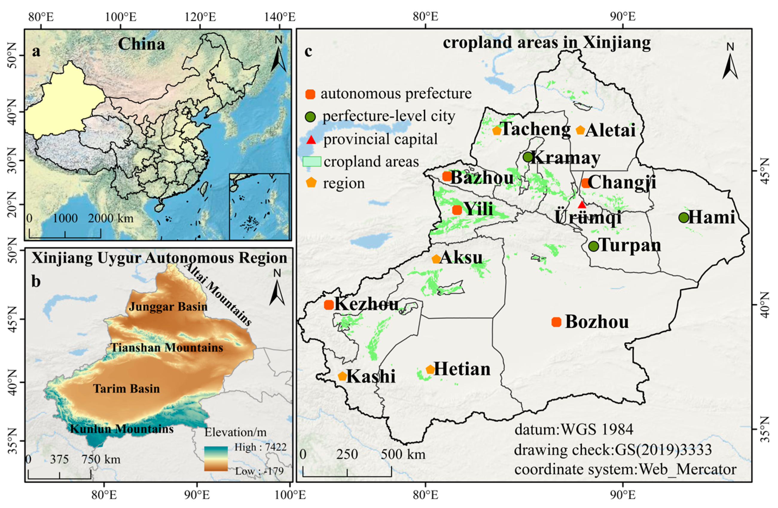
Figure 1. (a) Geographic location of Xinjiang. (b) Topographic features of Xinjiang. (c) The Xinjiang cropland region and the areas in which it is located.
Agronomy 15 01902 g001
Figure 2. Evaluation diagram of the XGBoost model. The evaluation results for R2, MAE, and RMSE metrics for the overall data, training set, and test set are displayed in the top-left corner. The red line represents the predicted values fitted by the model.
Agronomy 15 01902 g002
Figure 3. Inter- and intra-annual variations of WUEc in Xinjiang from 2002 to 2022, (a) the slope of the interannual trend component of WUEc, (b) intra-annual variations of WUEc, The color gradient from blue to red represents the change in years from 2002 to 2022.
Agronomy 15 01902 g003
Figure 4. Trends in annual mean (a) and Sen + MK test (b) for WUEc in Xinjiang, 2002–2022.
Agronomy 15 01902 g004
Figure 5. Spatial distribution of WUEc sustainability and stability in Xinjiang, 2002–2022, (a) spatial distribution of the Hurst index of WUEc in Xinjiang, (b) future evolutionary trend of WUEc in Xinjiang, and (c) spatial distribution of the CV coefficient of WUEc in Xinjiang.
Agronomy 15 01902 g005
Figure 6. Spatial distribution patterns of SHAP values for meteorological factors: (a) SHAP value distribution for temperature (T), (b) SHAP value distribution for precipitation (Pre), and (c) SHAP value distribution for vapor pressure deficit (VPD). Positive SHAP values indicate a positive effect on WUEc, while negative values indicate a negative effect.
Agronomy 15 01902 g006
Figure 7. Spatial distribution patterns of SHAP values for vegetation factors: (a) SHAP value distribution for the Enhanced Vegetation Index (EVI), and (b) SHAP value distribution for the Leaf Area Index (LAI). Positive SHAP values indicate a positive effect on WUEc, while negative values indicate a negative effect.
Agronomy 15 01902 g007
Figure 8. Contribution ranking of meteorological and vegetation factors (a) and the spatial distribution of their dominant regions (b).
Agronomy 15 01902 g008
Figure 9. The SHAP dependence plots illustrate how the SHAP values vary along the gradient of meteorological factors: SHAP dependence plot of T and WUEc (a), SHAP dependence plot of Pre and WUEc (b), and SHAP dependence plot of VPD and WUEc (c), SHAP dependence plot of LAI and WUEc (d), SHAP dependence plot of EVI and WUEc (e).
Agronomy 15 01902 g009
Table 1. Types and sources of data.
Data ClassificationData NameTemporal ResolutionSpatial ResolutionYearData Source
Land-use type dataCLCD1 year30 m2002–2022China Land Cover Dataset
Vegetation dataGPP/gC·m−21 month500 m2002–2022MODIS MYD17A2H
ET/mm1 month500 m2002–2022MODIS MOD16A2
EVI
LAI
1 year
1 year
1000 m
500 m
2002–2022MODIS MOD13A1
MODIS MOD13A1
Meteorological dataT/℃1 year1000 m2002–2022National Earth System
Science Data Center
Pre/mm1 year1000 m2002–2022National Earth System
Science Data Center
VPD/Kpa1 year1000 m2002–2022TerraClimate
Table 2. Statistical table of SHAP values and spatially dominant regions for meteorological and vegetation factors.
Factor Importance on WUEcTaLAIPreVPDEVI
Factor importance index (gC·mm−1·m−2)0.150.10.090.080.05
Proportion of dominant factor regions (%)45.717.617.414.74.6
Disclaimer/Publisher’s Note: The statements, opinions and data contained in all publications are solely those of the individual author(s) and contributor(s) and not of MDPI and/or the editor(s). MDPI and/or the editor(s) disclaim responsibility for any injury to people or property resulting from any ideas, methods, instructions or products referred to in the content.