Management Zones for Irrigated and Rainfed Grain Crops Based on Data Layer Integration

Abstract

This study investigates the delineation of management zones (MZs) to support site-specific crop management by simplifying within-field variability in irrigated (54.6 ha) and rainfed (7.9 ha) sorghum and soybean fields in Brazil. Historical yield, apparent soil electrical conductivity (ECa) at 0.75 m and 1.50 m, and terrain data were analyzed using multivariate statistics to define MZs. Two clustering methods—fuzzy c-means (FCM) and hierarchical clustering—were compared for variance reduction effectiveness. Rainfed areas showed greater spatial variability (yield CV 9–12%; ECa CV 20–27%) than irrigated fields (yield CV < 7%; ECa CV ~5%). Principal component analysis (PCA) identified subsoil ECa and elevation as key variables in irrigated fields, while surface ECa and topography influenced rainfed variability. FCM produced more homogeneous zones with fewer classes, especially in irrigated fields, whereas hierarchical clustering better detected outliers but required more zones for similar variance reduction. Yield correlated strongly with slope and moisture in rainfed systems. These results emphasize aligning MZ delineation with production system characteristics—enabling variable rate irrigation in irrigated fields and promoting moisture conservation in rainfed systems. FCM is recommended for operational efficiency, while hierarchical clustering offers higher precision in complex contexts.

1. Introduction

In contemporary agriculture, understanding the spatial and temporal variability of crop yields, soil physical and chemical properties, and the influence of environmental factors is essential for developing sustainable crop management strategies [1]. Precision agriculture (PA) is a management strategy that accounts for spatial and temporal variability to enhance the sustainability and efficiency of agricultural production [2].

Selecting optimal spatial resolution presents challenges in precision agriculture. Management zones (MZ) address the resolution–efficiency trade-off: finer resolutions detect microvariations but increase costs, while coarser resolutions improve efficiency. The approach’s effectiveness depends on the nature, causes, and agricultural application of observed variability. MZs are defined as subareas within a field that share similar characteristics, enabling uniform soil and crop management within each zone [3,4]. The primary objective of MZs is to support site-specific agricultural practices by identifying field areas where yield may be constrained and where differential management of inputs such as fertilizers, soil amendments, or seeds is required.

Aggregating historical data and converting them into actionable information is one of the key advantages of the MZ approach, as it simplifies site-specific management decision-making through spatial resolution simplification [4]. A tool for assessing spatial variability is geostatistics, which starts with the evaluation of spatial dependence through the semivariogram. It is also essential for determining the geostatistical predictor, such as interpolation by kriging [5]. This technique helps identify spatial patterns, supporting optimal resolution selection for crop management.

Numerous data layers and methodologies are available for delineating MZs. These include biotic, abiotic, and climatic variables as well as soil properties such as texture [6], soil organic matter content [7], and soil depth [8]. Additionally, terrain attributes derived from digital elevation models (DEMs) (e.g., elevation, slope) [9] are frequently employed as they directly influence yield. Yield maps, whether quantitative, qualitative, or integrated with other layers, also serve as valuable tools for delineating MZs [10]. Other commonly used data sources include remote sensing [11] and both invasive and noninvasive soil surveys—particularly those utilizing ECa sensors [12]. ECa sensors facilitate systematic data acquisition over large agricultural areas, providing detailed spatial continuity at a relatively low cost. Consequently, ECa data have become increasingly popular for MZ delineation [8,13]. ECa is particularly effective for detecting spatial variability related to moisture and clay content [14] as well as guide variable rate irrigation (VRI) recommendations, since these correlate with the soil’s water storage capacity or are applied by MZs, which define the response potential in areas of a field and, consequently, the crop’s differential water demand [15], and for guiding soil sampling strategies aimed at fertility assessment [16].

The complexity arising from interactions among soil attributes, climatic conditions, and crop responses presents significant challenges in defining zones with homogeneous productive potential [17]. Therefore, integrating multiple variables, particularly those with temporal stability and strong correlations with yields, is essential for effective MZ delineation [18]. Given the common issue of multicollinearity among variables, principal component analysis (PCA) is often applied to reduce dimensionality by transforming correlated variables into a smaller set of components that retain most of the data’s variance [19]. These principal components are subsequently used as inputs for the MZs delineation process [18].

Unsupervised clustering algorithms are the most widely adopted methods for MZ delineation when multiple variables are involved [20]. Among these, k-means and fuzzy c-means (FCM) clustering are particularly notable [10,21]. FCM employs an iterative process to partition data into clusters by computing centroids and membership degrees for each observation. Each data point is assigned to the cluster for which it exhibits the highest membership value, in a procedure known as defuzzification [22].

Hierarchical clustering, particularly using Ward’s method [23], is another effective approach for MZ delineation. Although computationally intensive, it is deterministic and produces a dendrogram that visually represents different clustering solutions. The method operates by minimizing within-cluster variance at each step of the agglomerative process, progressively merging clusters to reduce the sum of squared deviations [24].

Given the variability in outcomes depending on the chosen methodology, robust validation strategies are essential. One commonly used metric is variance reduction, which assesses how well the delineation minimizes within-cluster variability [25]. The principle is that aggregating areas with similar soil or yield characteristics should result in lower variance within each MZ. Lajili et al. [26] evaluate and compare the performance of different clustering techniques, including fuzzy k-means, iterative self-organizing data analysis technique (ISODATA), hierarchical clustering, and spatial segmentation.

Once the optimal number of MZs is identified, statistical tests are employed to assess whether the means of the attributes differ significantly between zones. These may include parametric tests such as analysis of variance (ANOVA) or nonparametric tests like Wilcoxon, Kruskal–Wallis [26], and Mann–Whitney [27]. Additionally, the Kappa index is frequently used to evaluate the spatial agreement between MZ maps and the original input data layers [20,22].

Given the lack of consensus on optimal methods for delineating MZs in grain production systems, the objective of this study is to compare FCM and hierarchical clustering methods for delineating MZs using yield maps, ECa, and terrain attributes in irrigated and rainfed grain fields.

2. Materials and Methods

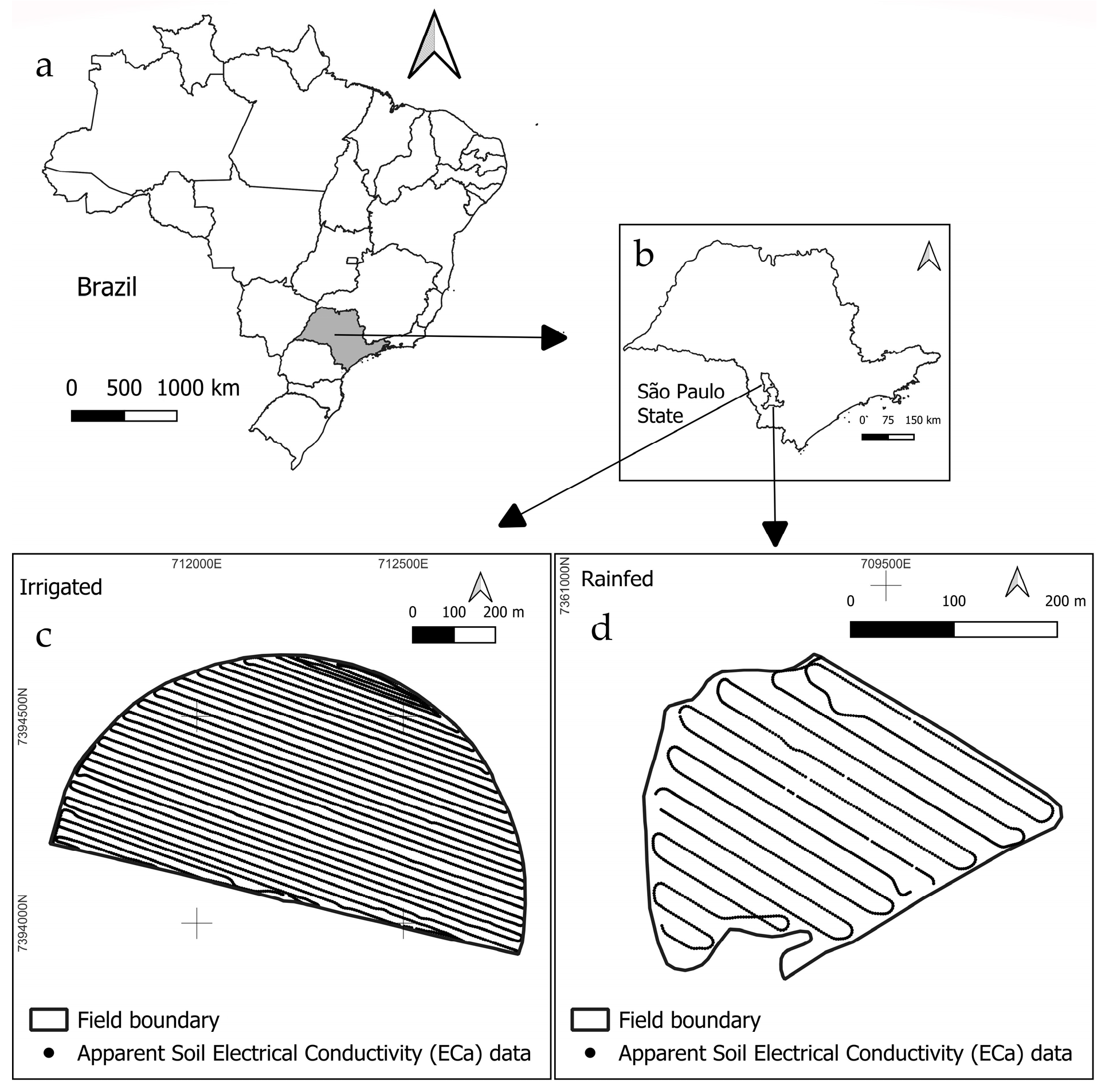
2.1. Study Areas

Two fields were selected for this study: one irrigated by center pivot with an area of 54.6 hectare (ha), located in the municipality of Itaí, São Paulo, Brazil (23°32′49″ S and 48°55′11″ W), and one rainfed field with an area of 7.9 ha, located in Itapeva, SP, São Paulo, Brazil (23°51′03″ S and 48°56′39″ W ). According to climate data from Climate Data [28], the climate in the areas is classified as Cfa (humid subtropical) according to Köppen and Geiger [29].

The slope of the irrigated field is predominantly classified as flat (<3%), with an average elevation of 665 m. In the rainfed field, the terrain is mainly classified as gently undulating (3–8%), with an average elevation of 674 m [30] (Figure 1).

2.2. Data Characterization

The sorghum and soybean yield data were obtained from combine harvesters equipped with yield monitors, collected between 2019 and 2025. The header cutting width was 9.1 m, with a data acquisition frequency of 1 Hz. The yield data point density ranged from 696.2 to 1150.6 points per hectare. Irrigated soybeans occurred in 2019–2025 (except 2020), with sorghum added in 2024. Under-rainfed soybean was grown in 2019–2021 and 2023, while sorghum appeared in 2020 and 2022.

ECa was measured using the electromagnetic induction (EMI) sensor EMP-400 (Geophysical Survey Systems, Inc.—GSSI, Nashua, NH, USA), providing data up to ~1.5 m depth. The sensor operated 20 m behind the tractor, logging data every second, with RTK GNSS positioning (John Deere/StarPAL HGIS v10.0). The measurement setup records two depth profiles: 0–0.75 m and 0–1.50 m, with data collected at 20 m spacing between rows (Figure 1). Measurements were taken in March 2017 (irrigated area: 4918 points) and April 2025 (rainfed area: 1443 points).

The elevation data were extracted from the SRTM mission DEM. The OpenTopography plugin in QGIS [31] was used to obtain elevation data. The raster layer, in GEOTIFF image format, was loaded for the extent of the fields of interest. From the DEM, the slope (%) was calculated.

2.3. Data Filtering, Statistical and Geostatistical Analysis

Yield and ECa raw data were filtered using MapFilter software version 2.0 [32]. This software allows statistical filtering to remove gross errors, also known as outliers, followed by spatial filtering through a comparative evaluation of yield values from neighboring points. Upper (LimS) and lower (LimI) limits were established using the median for filtering, defined as:

$$LimS=MK+MK\cdot v$$

(1)

$$LimI=MK-MK \cdot v$$

(2)

where $LimS$: upper limit; $LimI$: lower limit; $MK$: median of all values in the dataset; $v:$ maximum accepted variation for the median.

The input parameters for filtering the yield data were 50% as accepted ($v$) for the statistical filtering and 75% for the local filtering, with a spatial dependence of 91 m, which is ten times the width of the harvester platform. For the ECa data, the input parameters were 50% as accepted ($v$) for statistical filtering, 20% for local filtering, and a spatial dependence of 200 m, ten times the distance between measurement rows.

After filtering, the ECa and yield data were interpolated using geostatistical parameters, generating spatial images (raster) with a resolution of 3 m. For semivariogram calculation and kriging, the smart-map plugin of QGIS was used [33]. The model fitting was based on the highest coefficient of determination (R²) and the lowest root mean square error (RMSE) obtained by cross-validation. Additionally, the following parameters were defined for each model: maximum distance between pairs of points to be analyzed to determine spatial dependence, lag (interval or step tolerance), nugget effect (C₀), structural component (C₁), sill (C₀ + C₁), range (a), and radius considered for interpolation (

Table 1. Semivariogram models and fitting parameters used for spatial interpolation in SmartMap software (version 1.4.2) for irrigated and rainfed fields.

Irrigated
Attribute	Model	Max_dist (m)	Lag (m)	C0	C0 + C1	Range (m)	RMSE	R2	DSD (%)	DSD Class
ECa 0.75 m	Linear with Sill	694.7	6.6	8.15	26.75	691.1	37.42	0.99	30.45	Moderate
ECa 1.50 m	Linear with Sill	694.7	6.6	26.89	87.74	605.5	353.48	0.99	30.65	Moderate
Soybean 2019	Linear with Sill	750.0	12.8	0.38	0.60	746.7	0.02	0.91	63.71	Moderate
Soybean 2021	Gaussian	696.6	12.7	0.19	0.31	691.5	0.01	0.94	62.21	Moderate
Soybean 2022	Linear with Sill	696.2	12.7	0.18	0.26	691.1	0.00	0.91	69.96	Moderate
Soybean 2023	Exponential	697.5	12.7	0.09	0.31	397.3	0.01	0.93	28.80	Moderate
Soybean 2024	Spherical	692.9	12.7	0.17	0.36	639.3	0.00	0.99	45.88	Moderate
Sorghum 2024	Exponential	696.1	12.7	0.04	2.65	585.9	0.17	0.99	1.36	Strong
Soybean 2025	Spherical	696.7	12.7	0.27	0.63	592.3	0.02	0.97	43.35	Moderate
Rainfed
Attribute	Model	Max_dist (m)	Lag (m)	C0	C0 + C1	Range (m)	RMSE	R2	DSD (%)	DSD Class
ECa 0.75 m	Linear	150.0	15.0	0.00	74.04	101.8	1601.95	0.90	0.00	Strong
ECa 1.50 m	Spherical	140.0	10.0	2.42	66.75	135.5	37.48	0.99	3.63	Strong
Soybean 2019	Exponential	200.0	2.4	0.34	0.79	130.1	0.08	0.93	43.04	Moderate
Soybean 2020	Exponential	200.0	2.0	0.14	0.65	53.3	0.09	0.91	20.71	Strong
Sorghum 2020	Linear	170.0	6.7	0.93	1.36	98.0	0.06	0.95	68.39	Moderate
Soybean 2021	Linear	241.4	2.0	0.63	1.00	127.8	0.68	0.88	62.70	Moderate
Sorghum 2022	Spherical	160.0	6.9	0.18	0.38	158.6	0.00	0.98	46.19	Moderate
Soybean 2023	Exponential	240.8	2.3	0.46	1.22	240.3	0.54	0.88	37.35	Moderate

Max_dist: maximum distance between point pairs; C₀: nugget effect; C₁: structural component; C₀ + C₁: sill.

). A radius equal to the range and 16 neighbors were used. The degree of spatial dependence (DSD) of the variables was calculated and classified according to Cambardella et al. [34] as follows: DSD ≤ 25%—strong; 25 < DSD ≤ 75%—moderate; and DSD > 75%—weak.

The study utilized a regular grid of points (pixel centroids) at a 3 m resolution, generated after kriging. Raster values were sampled for variables such as ECa, yield, terrain attributes, and geographic coordinates. An exploratory data analysis was conducted to assess the spatial variability of the attributes, including mean, standard deviation, coefficient of variation (CV%), maximum and minimum values, skewness, and kurtosis. Data normality was evaluated using the Anderson–Darling (A²) test at a 5% significance level, while variability was classified according to Wilding [35] as high (CV > 35%), moderate (CV between 15% and 35%), or low (CV < 15%).

Following the delineation of MZs, parametric (ANOVA, p-value < 0.05) and nonparametric tests (Kruskal–Wallis with Dunn’s post-hoc) were applied based on data distribution, comparing means or medians across MZs. These analyses were restricted to cases with at least three MZs to meet test assumptions. Boxplots were generated to visualize data distribution.

Finally, Spearman’s rank correlation analysis was performed to evaluate monotonic relationships between variables, as this method does not require assumptions of normality or linearity [36]. Spearman’s coefficients (rs) were interpreted according to Rumsey [37], where |rs| = 1 indicated a perfect linear relationship, |rs| ≥ 0.70 a strong relationship, |rs| ≥ 0.50 a moderate relationship, and |rs| ≥ 0.30 a weak relationship. This step helped quantify the influence of the studied factors on yield, contributing to a better understanding of spatial variability.

2.4. Multivariate Statistics and MZs Delineation Methods

In this stage of principal component analysis (PCA), the sampled points mentioned in the previous item were used. Therefore, each point contains information on yield, apparent ECa at two depths, and terrain attributes. The data were standardized using Z-score normalization. PCA was applied using the criterion of accumulated variance ≥80% for selecting the number of components.

The delineation of MZs was performed through cluster analysis using the FCM algorithm [38], applied to the factor score matrix of selected principal components (PCs).

$$J_m=\sum _{i=1}^N\sum _{j=1}^C{u}_{ij}^m\cdot {{||x}_i-c_j||}^2$$

(3)

where N: number of data points; C: number of clusters; U_ij: membership degree of data point x_i to cluster j; m: fuzziness parameter; x_i: feature vector of the i-th observation; c_j: centroid of cluster j; ${{||x}_i-c_j||}^2:$ squared Euclidean distance. The parameters used were C = number of clusters to generate; m = 1.2: fuzzy exponent; error = 0.005: convergence criterion; maximum number of iterations = 1000.

Comparatively, hierarchical agglomerative clustering was used. The “ward” linkage method was used to compute the linkage matrix Z. The Ward distance between two clusters A and B is given by

$$D\left(A,B\right)={\displaystyle \frac{\left|A\right|\left|B\right|}{\left|A\right|+\left|B\right|}}\cdot |\overline{x_A}-\overline{x_B}{|}^2$$

(4)

where $\left|A\right| \mathrm{and} \left|B\right|: \mathrm{sizes} \mathrm{of} \mathrm{clusters} A \mathrm{and} B; \left(\overline{x_A}\right) \mathrm{and} \left(\overline{x_B}\right)$: centroids of A and B; |⋅|: Euclidean distance.

The generation of cluster labels is based on the definition of a maximum number of groups. For FCM and hierarchical methods, the number of clusters from 2 to 10 was generated.

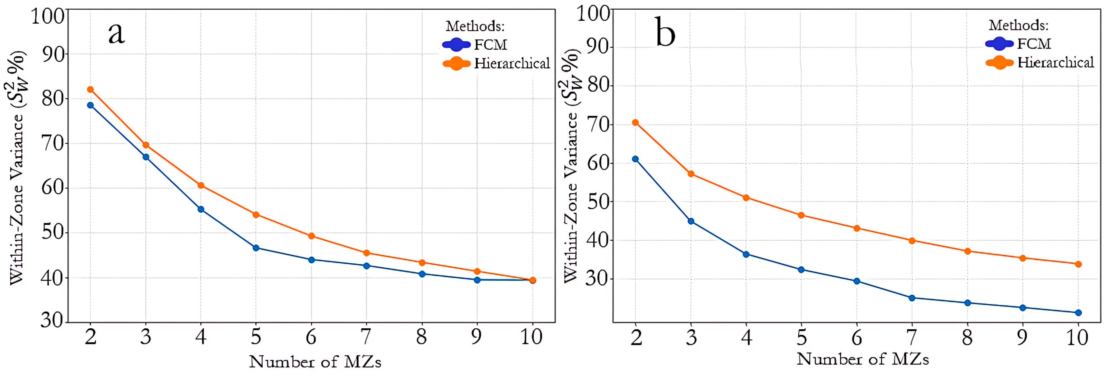
2.5. Evaluation of MZs Separation

A multivariate analysis of variance was employed to assess the homogeneity of the MZs identified by the applied algorithms. This approach considered all selected variables together, allowing for an integrated evaluation of data variability. The total variance was calculated as a measure of the overall dispersion of the data before clustering, representing the natural variability present in the entire dataset. After the clusters were formed, the within-cluster variance was calculated, quantifying the residual dispersion within each individual MZ.

To evaluate clustering effectiveness, two metrics were used: the variance reduction (VR%) and the within-cluster variance percentage ($S_W^2$). The former indicates how much of the total variability was explained by the formation of MZs, while the latter shows the proportion of variability that remains within the formed clusters.

$$\mathrm{VR} \left(\%\right)=\left(1-{\displaystyle \frac{S_W^2}{S_T^2}}\right)\times 100$$

(5)

where $\mathrm{VR} \left(\%\right)$: variance reduction (%); $S_W^2$: within-MZ variance; $S_T^2$: total variance of the area.

To calculate the percentage of $S_W^2$ a modified version of Equation (5) was used:

$$Relative within-MZ variance (\%)= \left({\displaystyle \frac{S_W^2}{S_T^2}}\right)\times 100$$

(6)

3. Results and Discussion

3.1. Data Filtering

Data filtering was a necessary step to remove inconsistencies and outliers commonly present in raw yield monitor data. The reduction in the total number of yield points ranged from 4.0% (irrigated soybean 2024) to 31.6% (rainfed soybean 2019), reflecting differences related to field conditions, cropping systems, and harvest years. Most fields showed reductions between 4% and 10%, while rainfed areas experienced more substantial losses, exceeding 17%, due to the greater spatial variability typically observed under these conditions. Although numerically significant in some cases, data filtering improved overall data quality, resulting in an increase in mean yield and a substantial reduction in standard deviation—by approximately 50%.

Regarding apparent soil electrical conductivity (ECa), data point removal was more intense in rainfed areas, ranging from 26.5% to 37.4%, while irrigated areas showed minimal reductions (0.3%). Mean ECa values increased in rainfed fields (e.g., from 40.2 to 41.0 mS m⁻¹ at 0–0.75 m depth and from 50.9 to 60.9 mS m⁻¹ at 0–1.50 m), whereas irrigated fields experienced minor decreases. The standard deviation of ECa decreased in irrigated areas (e.g., from 4.5 to 3.1 mS m⁻¹ in 2017 at 0–0.75 m depth), with more notable reductions at 0–1.50 m depth in rainfed fields.

3.2. Geostatistic

Different theoretical models (linear, linear with sill, spherical, exponential, and Gaussian) were fitted to describe the spatial dependence structure of the attributes, revealing notable variations across variables. Linear with sill models predominated for ECa (e.g., ECa at 0.75 m and 1.50 m), while exponential, spherical, and occasionally Gaussian models were more common for soybean yield (e.g., soybean 2021—Gaussian; soybean 2024—spherical).

The range varied substantially, from 53.3 m (soybean 2020—rainfed) to 746.7 m (soybean 2019—irrigated), reflecting differences in field size (54.6 ha irrigated vs. 7.9 ha rainfed). The nugget effect (C₀) also displayed considerable variation, with higher values for ECa (e.g., 26.89 mS m⁻¹ at 1.50 m depth), indicating unresolved microvariability, and lower values for yield (e.g., 0.04 Mg ha⁻¹ for sorghum 2024—rainfed), suggesting high sampling precision. The sill (C₀ + C₁) followed the same pattern, reaching maximum values for ECa (up to 87.74 mS m⁻¹) and minimum values for yield (0.26 Mg ha⁻¹ in soybean 2022).

Irrigated fields generally exhibited larger ranges (e.g., 691.1 m for ECa at 0.75 m; 746.7 m for soybean 2019) compared to rainfed areas (e.g., 101.8 m for ECa at 0.75 m; 53.3 m for soybean 2020). Nugget values were also higher in irrigated areas for ECa (26.89 mS m⁻¹ vs. 0.00 mS m⁻¹ in rainfed), while rainfed fields showed negligible nuggets for yield, emphasizing adequate sampling resolution.

The degree of spatial dependence (DSD) was predominantly moderate, with distinctions between systems and crops. In irrigated soybean, DSD ranged from 28.8% to 69.9% (moderate), whereas sorghum exhibited strong spatial dependence (1.36%). ECa in irrigated areas was classified as moderate, while in rainfed areas, ECa displayed strong spatial dependence, and soybean yield remained moderately dependent across years. Sorghum under rainfed conditions ranged from moderate to strong DSD (Table 1).

3.3. Descriptive Statistics of the Attributes

The sampled points (N) from the kriging-interpolated and DEM raster data—N = 60,670 for irrigated fields and N = 8811 for rainfed fields—were statistically analyzed, and the results for each field are summarized in

Table 2. Results of the descriptive statistical analysis of the variables.

Irrigated
	Min	Mean	Max	SD	CV (%)	S	K	Var
Slope	0.7	2.6	17.2	1.2	47.3	3.95	30.55	high
Elevation	659.2	666.1	673.3	3.5	0.5	−0.01	−1.02	low
ECa 1.50 m	93.1	111.7	127.7	6.1	5.4	−0.26	−0.43	low
ECa 0.75 m	54.2	63.3	74.9	3.1	5.0	−0.39	0.09	low
Sorghum 2024	3.8	6.7	9.1	1.4	21.0	0.25	−1.42	moderate
Soybean 2025	6.4	8.1	9.4	0.5	6.3	−0.11	−0.17	low
Soybean 2024	5.3	6.8	7.4	0.4	5.4	−1.15	0.94	low
Soybean 2023	5.2	6.5	7.7	0.4	6.5	0.33	−0.13	low
Soybean 2022	6.3	7.5	8.1	0.2	3.2	−0.45	1.09	low
Soybean 2021	6.7	7.9	8.6	0.3	3.5	−0.89	0.86	low
Soybean 2019	4.5	6.9	7.7	0.4	6.3	−1.48	3.98	low
Rainfed
	Min	Mean	Max	SD	CV (%)	S	K	Var
Slope	0.7	5.9	11.9	2.4	40.0	−0.09	−0.71	high
Elevation	663.1	672.4	683.0	4.2	0.6	0.28	−0.88	low
ECa 1.50 m	35.8	55.3	76.8	10.8	19.5	−0.29	−1.28	moderate
ECa 0.75 m	22.2	40.4	60.4	10.9	26.9	−0.10	−1.23	moderate
Sorghum 2022	2.5	3.6	4.7	0.4	12.0	−0.12	−0.45	low
Sorghum 2020	5.6	8.2	10.9	0.9	10.7	−0.14	−0.08	low
Soybean 2023	4.8	6.8	9.3	0.8	11.5	0.29	−0.57	low
Soybean 2021	4.6	8.1	10.1	0.8	9.4	−0.96	1.09	low
Soybean 2020	3.7	6.1	8.1	0.7	11.1	−0.58	−0.02	low
Soybean 2019	3.7	5.6	7.4	0.6	11.6	−0.24	−0.61	low

Min: minimum; Mean: average; Max: maximum; SD: standard deviation; S: skewness; K: kurtosis; Var = variability.

. The analysis of topographic attributes and ECa revealed clear differences between irrigated and rainfed systems. In the irrigated area, slope exhibited high variability (CV = 47.3%) with pronounced skewness and kurtosis, indicating steep gradients that could reduce irrigation efficiency by increasing runoff risk. In contrast, the rainfed area showed slopes with a CV of 40.0% and a mean value of 5.9%, which may affect rainwater retention. Elevation and slope, derived from SRTM digital models, can be influenced by nearby vegetation or structures, particularly at field edges (e.g., a forest adjacent to the irrigated field affected elevation values).

For ECa, the irrigated system displayed low variability (CV ~5% at both depths), reflecting soil moisture homogeneity due to irrigation, whereas the rainfed system showed moderate variability (CV = 19.5–26.8%), indicating greater natural heterogeneity. Irrigation also reduced yield variability: sorghum in irrigated areas showed moderate variability (CV = 21.0%), likely due to localized soil or management differences, whereas rainfed sorghum was more stable (CV = 10–12%) due to the crop’s resilience. Soybean under irrigation exhibited high yield stability (CV < 7%), while rainfed soybean had greater variability (CV = 9–12%), possibly influenced by water availability.

The Anderson–Darling test (α = 0.05) confirmed non-normal distributions for all variables, as supported by high skewness (e.g., slope in irrigated field, S = 3.95) and kurtosis (K = 30.55) (Table 2).

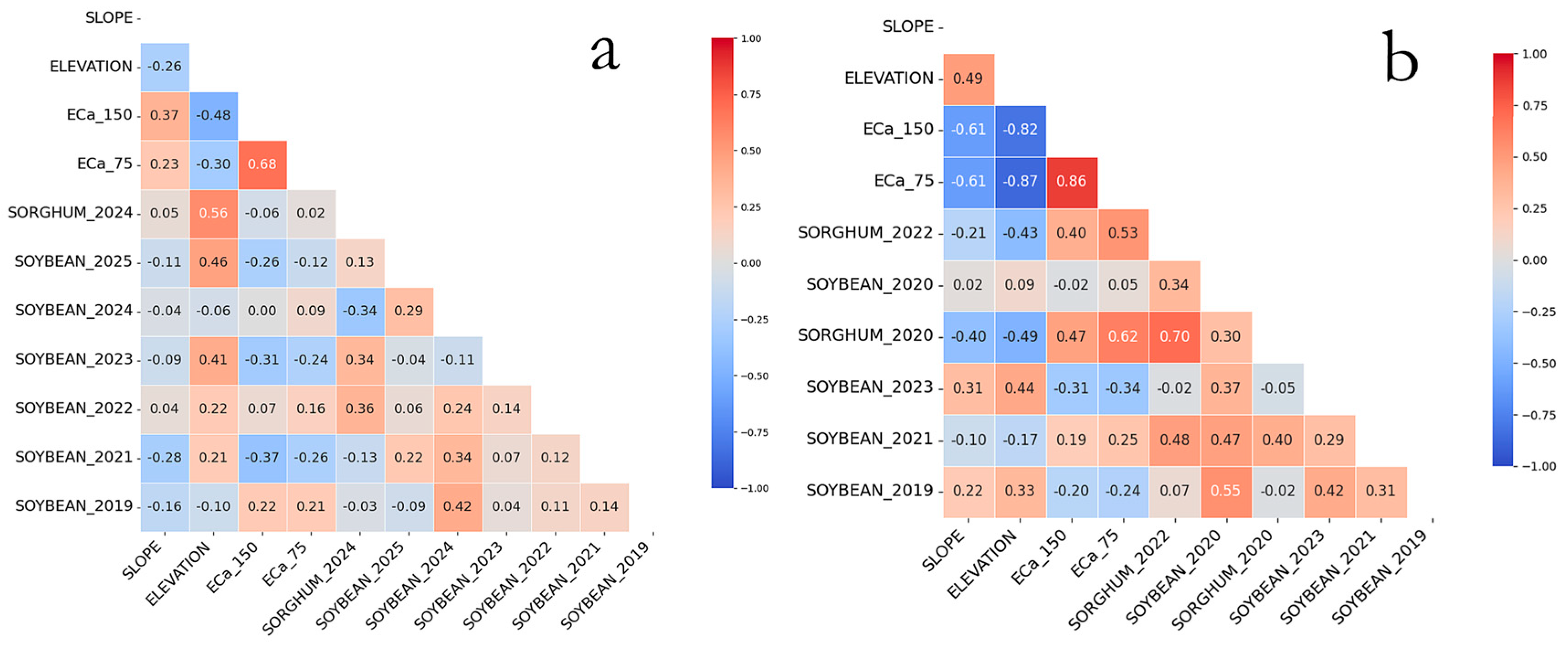
3.4. Spearman Correlation

The correlation analyses revealed marked differences between the two production systems. In the irrigated system, slope had little influence on yield, with negligible correlations, suggesting that irrigation mitigates the adverse effects of topography. Interestingly, higher elevations were associated with increased sorghum yields (r = 0.56), possibly due to improved drainage conditions. ECa showed a moderate correlation between soil layers (r = 0.68) but exhibited only a weak association with yield.

In the rainfed system, distinct patterns emerged. Slope showed a moderate negative correlation with ECa (r = −0.61), indicating that flatter areas retain more moisture. This relationship was mirrored in yield patterns, with sorghum performing better in areas with lower slopes (r = −0.40 and −0.21), while soybean exhibited variable responses depending on the crop year. Elevation demonstrated a strong negative correlation with ECa (ranging from −0.82 to −0.87), suggesting that lower-lying areas tend to accumulate more moisture and salts. Regarding yield, sorghum benefited from higher ECa values (r = 0.40 and 0.62), whereas soybean showed negative correlations in some years (ranging from −0.31 to −0.34), likely due to its sensitivity to excessive soil moisture.

Yield analyses also revealed greater temporal stability in the irrigated system, with weak interannual correlations, while in the rainfed system, yields were more dependent on climatic conditions, showing moderate correlations between similar cropping years (r = 0.70 for sorghum). These results underscore the need for differentiated management strategies: in irrigated systems, efforts should focus on optimizing water application within each MZ using variable rate irrigation (VRI), while in rainfed systems, management must account for the spatial variability of soil properties and seasonal climatic fluctuations. Overall, this study highlights how water availability modulates soil–plant–climate interactions and reinforces the importance of tailoring agricultural practices to each production system (Figure 2).

3.5. Principal Component Analysis (PCA)

Six principal components (PCs) were required to explain ≥80% of the total variability in the irrigated area, whereas only four PCs were sufficient in the rainfed area. In the irrigated system, PC1 accounted for 27.9% and PC2 for 20.3% of the total variance, together explaining 48.2%. In contrast, in the rainfed system, PC1 captured 41.3% and PC2 24.8%, totaling 66.1% of the variance. This indicates a more defined structure in the rainfed dataset, with a larger proportion of variability concentrated in the first two components.

In the irrigated area, ECa at 0.75 m and 1.50 m depths, along with slope, contributed distinctly to PC2, suggesting these factors drive spatial differentiation under conditions not directly tied to yield. In the rainfed system, elevation and slope were strongly aligned and negatively associated with PC1, indicating that topographic features are critical for explaining yield variation where water availability is more dependent on terrain. The separation of yield vectors (e.g., soybean 2020 vs. sorghum 2024) further underscores interannual and crop-specific responses to environmental and management factors.

The dispersion of sample points and clustering of vectors suggest that, in irrigated areas, variability is more influenced by subsoil- and management-related variables (such as ECa). By contrast, in rainfed systems, terrain attributes like slope and elevation play a predominant role in shaping MZs (Figure 3).

In the irrigated area, the first principal component (PC1) was primarily influenced by elevation (19.9%) and ECa at 1.50 m (17.3%), followed by ECa at 0.75 m (11.3%). These results suggest that spatial variability in this system is strongly associated with topographic factors [9], soil texture [12,14], and its capacity to retain moisture [8,13], potentially reflecting the effects of irrigation water distribution. The second principal component (PC2) was mainly driven by soybean yield in 2024 (29.2%) and 2019 (24.7%), indicating that a substantial portion of the remaining variability is related to temporal variability in crop yield.

In contrast, in the rainfed area, PC1 showed the highest contribution from ECa at 0.75 m (22.0%), followed by ECa at 1.50 m (19.2%) and elevation (19.0%). This highlights that the primary source of variability is associated with soil texture and its capacity to retain moisture, along with topographic effects. These findings underscore the critical role of water retention in rainfed systems. PC2 was predominantly influenced by soybean yield in 2020 (26.4%) and 2019 (18.7%), suggesting that the secondary source of variability is related to the crop’s temporal variability responses to climatic conditions, particularly rainfall (

Table 3. Percentage of variance explained by principal components 1 and 2 (PC1 and PC2) for key variables in irrigated and rainfed systems.

Variable	PC1—Irrigated (%)	PC2—Irrigated (%)	PC1—Rainfed (%)	PC2—Rainfed (%)
Elevation	19.9	3.4	19.0	1.3
ECa 1.50 m	17.3	4.0	19.2	0.5
ECa 0.75 m	11.3	6.2	22.0	0.1
Soybean 2024	-	29.2	-	-
Soybean 2019	-	24.7	-	18.7
Soybean 2020	-	-	-	26.4

).

These results may have important agronomic implications. In irrigated systems, irrigation management could account for terrain attributes to adjust water application rates (VRI). Previous studies suggest that management zones (MZs) for precision irrigation can potentially reduce water and energy inputs, increase crop water productivity, minimize deep percolation and runoff, decrease fertilizer and other chemical inputs, and mitigate soil pollution [39].

In rainfed systems, management practices might focus on enhancing soil water retention, for example, adopting no-till practices and maintaining soil cover, to help buffer the effects of climatic variability on crop yield.

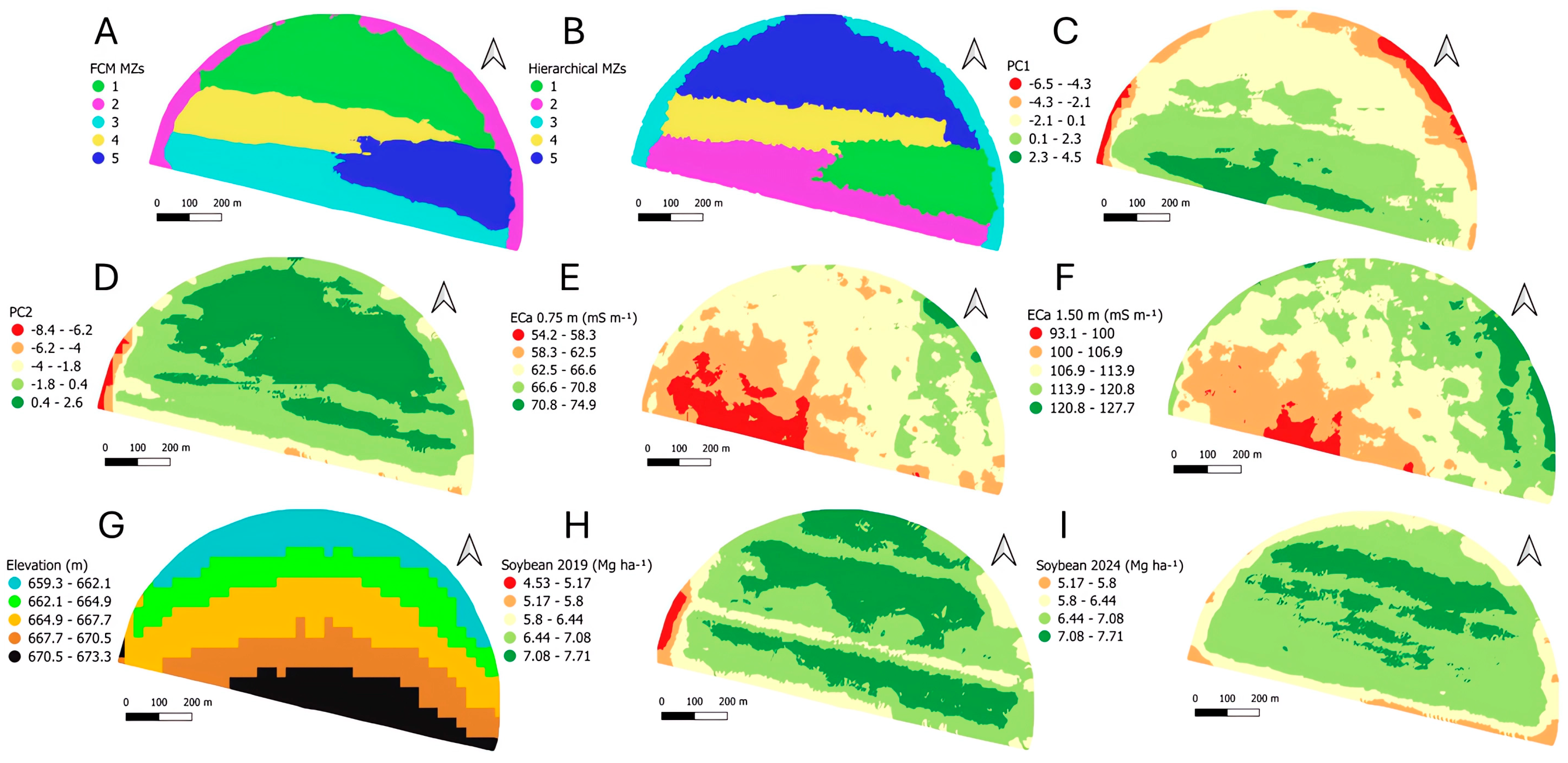
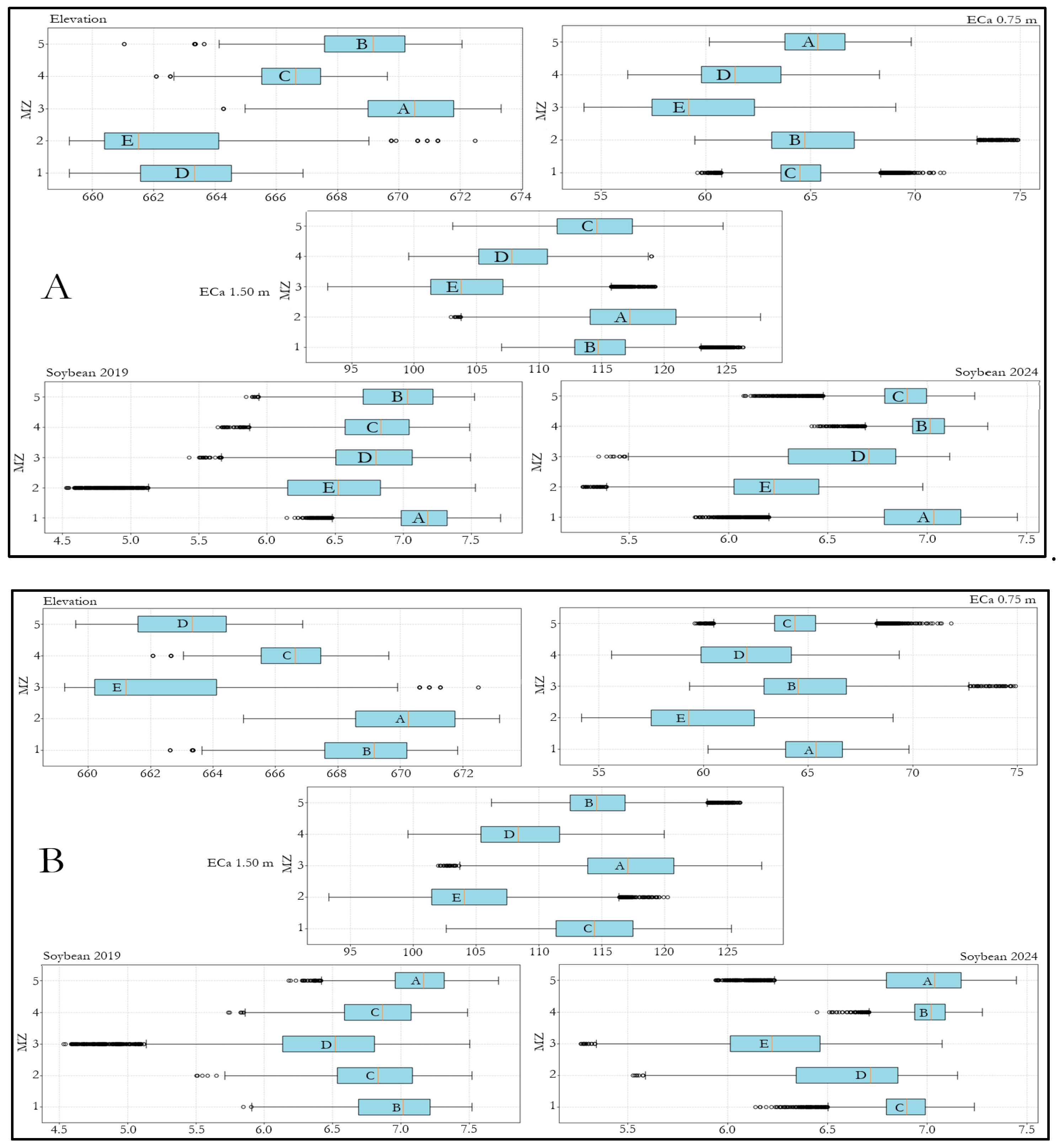
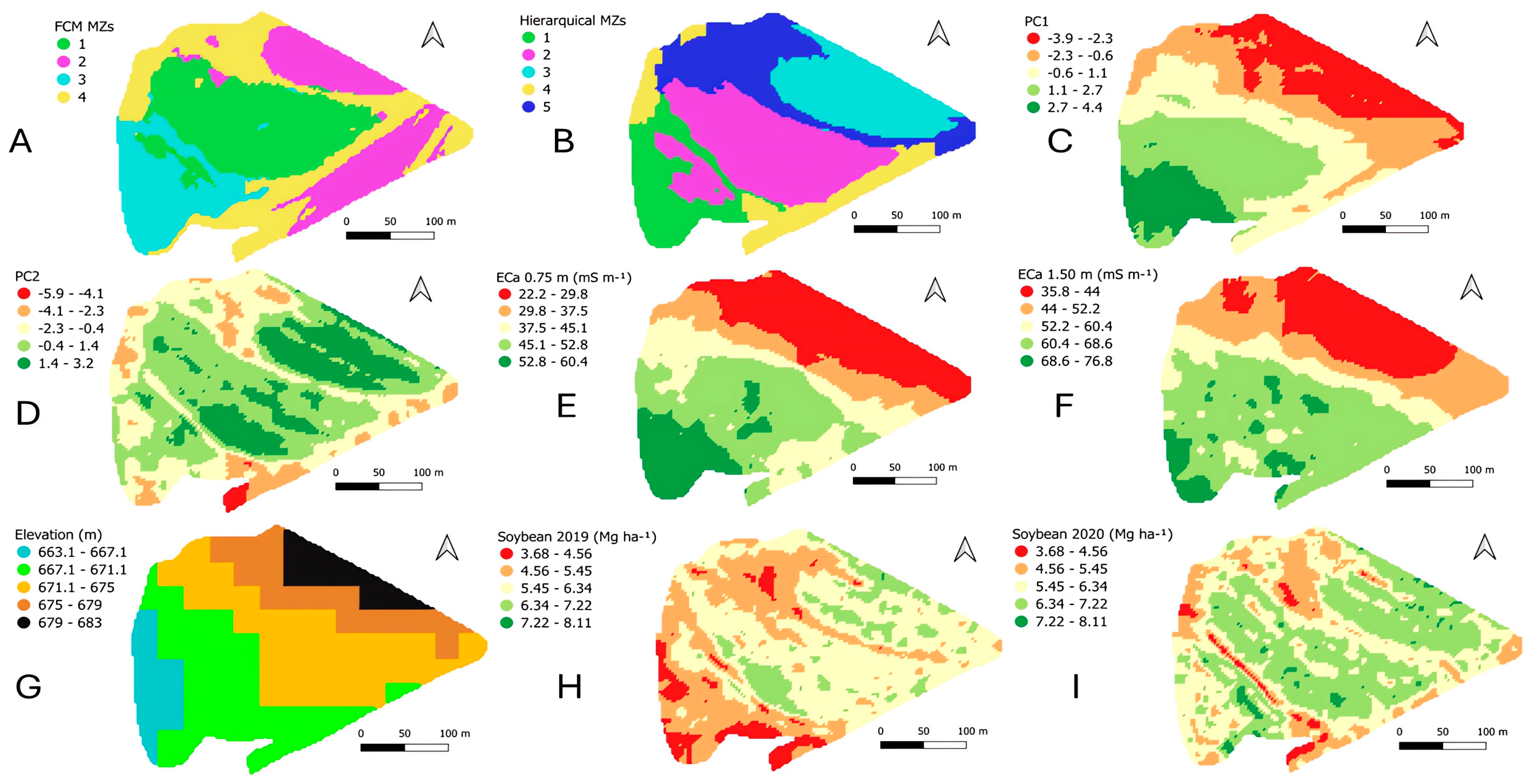
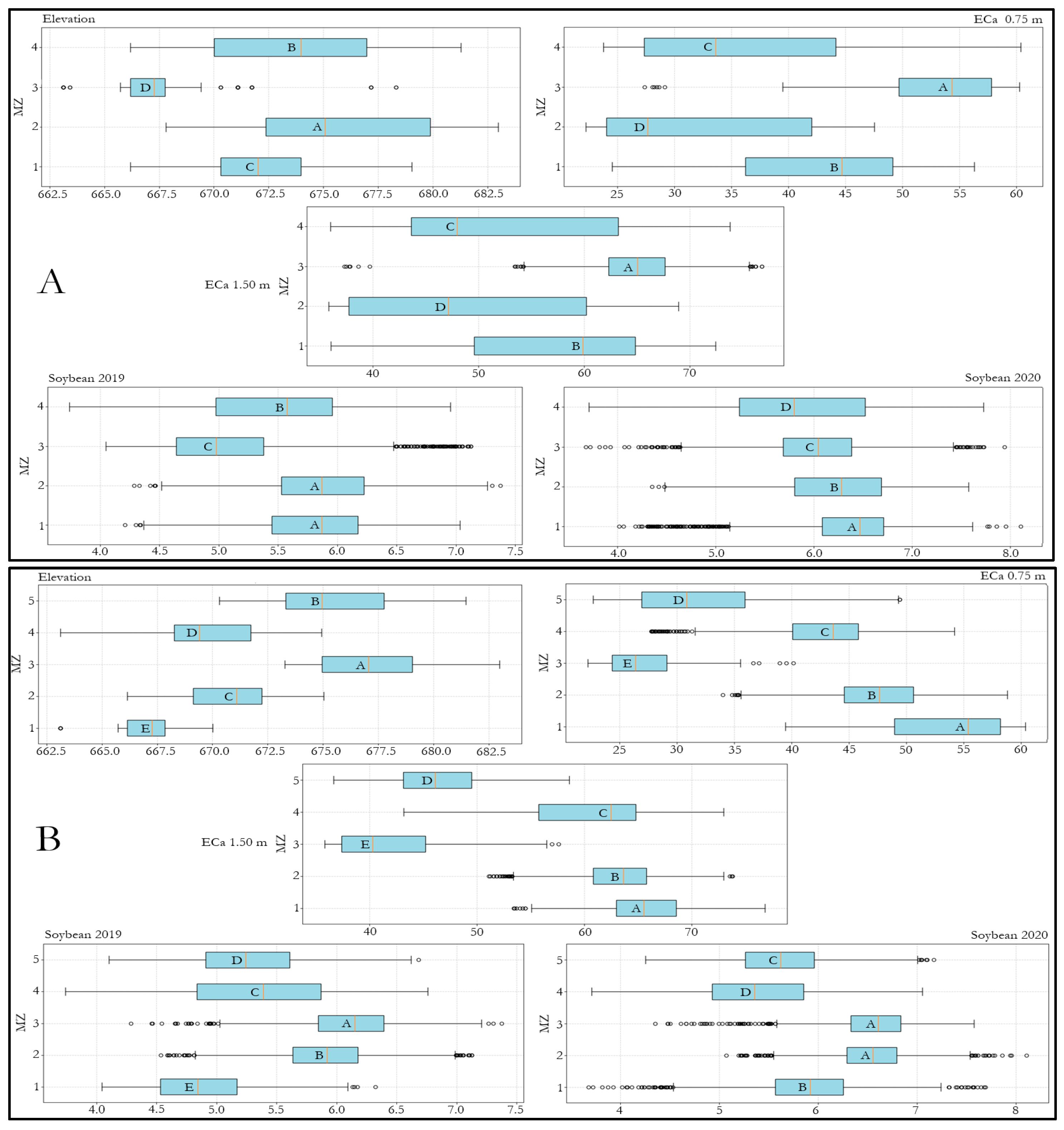
3.6. MZs Delineation

According to Figure 4, for the irrigated area, the optimal number of management zones (MZs) was five, as it balances variance reduction (VR = 53.38%) and residual variance ($S_W^2$ = 46.62%) for FCM, indicating strong homogeneity without excessive subdivision. Increasing from MZ = 4 to MZ = 5 yields a significant VR gain (+8.63 percentage points), while further increments (e.g., MZ = 5 to MZ = 6) provide diminishing returns (+2.62 points). Beyond MZ = 7, clusters become overly specific, whereas fewer than four zones may mask important patterns. Hierarchical clustering supports MZ = 5 as the point of explanatory efficiency, capturing $S_W^2=$54.12% and VR = 45.88% before marginal gains decline (<3% beyond MZ = 7).

In the rainfed area, for FCM, MZ = 4 was the optimal number of clusters, achieving 63.63% VR ($S_W^2$ = 36.37%) with the highest marginal gain (+8.55% vs. MZ = 3). While MZ = 5 offers finer detail (VR = 67.69%), the improvement diminishes (+4.06%). For the hierarchical method, the variance reduction occurs in three phases: (1) initial (MZ = 2–4): sharp $S_W^2$ decline (70.58% → 51.06%, ΔVR ~9.76% per increment); (2) intermediate (MZ = 4–7): slower reduction (51.06% → 39.91%, ΔVR ~3.72%); (3) final (MZ > 7): minimal gains (ΔVR < 2.5%). MZ = 5 remains viable (VR = 53.56%, $S_W^2$ = 46.44%), but MZ = 4 may be preferred for operational simplicity (VR = 48.94%).

The analysis of the algorithm’s efficiency in forming MZs in the irrigated area demonstrated that both FCM and hierarchical clustering were effective in delineating zones with low internal variability (CV) for the main attributes contributing to the first two principal components. However, FCM outperformed in ensuring greater homogeneity within MZs, as evidenced by lower CVs, particularly for soybean 2024 (1.75% (MZ 4, N = 11,397) to 5.56% (MZ 3, N = 12,180)) and ECa 0.75 m (2.51% (MZ 1, N = 19,986) to 5.18% (MZ 3, N = 12,180)). This result reinforces the robustness of fuzzy models in smoothing spatial transitions through gradual point assignment [38].

In contrast, hierarchical clustering was more sensitive to outliers and transition areas, reflected in higher CVs, such as soybean 2019 in MZ 3 (10.56%) and ECa 1.50 m (4.61%), with N = 3167. Given the hierarchical algorithm’s limitations in this area, the original dataset of 60,670 sampled points was reduced through resampling to 30,000 points.

Another key observation was the influence of field borders on MZ formation (Figure 5). In both methods, zones associated with borders showed lower yields and higher variability—for instance, in FCM, MZ 2, N = 6133, presented yields of 6.2 Mg ha⁻¹ (soybean 2024) and 6.4 Mg ha⁻¹, with a CV of 10.82% (soybean 2019). Similarly, in hierarchical clustering, MZ 3, N = 3167, had a CV of 10.56% (6.4 Mg ha⁻¹ for soybean 2019) and the same low yield for soybean 2024 (6.2 Mg ha⁻¹). This reinforces that border areas naturally concentrate spatial noise due to machinery maneuvers and soil compaction. Segregating these areas into specific MZs reduces their impact on the homogeneity of productive zones.

The statistical comparison of medians among MZs (Figure 6) confirmed significant differences, supporting the spatial stratification of yield. For instance, in FCM, soybean 2024 yield in MZs 1 (A) and 4 (B) significantly differed from MZs 2 (E) and 3 (D). Similarly, in the hierarchical method, ECa 1.50 m in MZ 3 (A) was significantly higher than in MZ 2 (E), highlighting distinct spatial patterns. Importantly, defining a specific MZ for borders enhanced the robustness of the analysis by isolating heterogeneous areas and improving the reliability of productive zone delineation.

For the rainfed area, the analysis of within-cluster variability showed that the hierarchical method with five zones provided greater internal homogeneity, with low coefficients of variation (CV < 15%) for most attributes. The exception was ECa 0.75 m in MZ 5 (CV = 18.2%, N = 1.845), reflecting the high sensitivity of this attribute to edaphic and environmental factors, such as texture, moisture, and organic matter [12].

FCM needed four zones to achieve good homogeneity for elevation and soybean yield (CV < 14%) but showed higher variability for ECa, especially in MZ 2 (ECa 0.75 m, CV = 27.2%). This is inherent to the probabilistic nature of the algorithm, which allows partial membership and offers greater flexibility in data allocation [38]. While this can reduce precision, it simplifies management by reducing the number of zones (Figure 7).

Statistical comparison of medians confirmed that both methods generated distinct MZs for elevation and ECa. However, for soybean yield, the hierarchical method showed redundancy, with no significant difference between MZs 2 and 3 in 2020. This suggests that five zones may be excessive for some attributes, adding complexity without proportional agronomic benefits (Figure 8).

Thus, the choice between FCM and hierarchical methods should balance the need for precision and operational feasibility. The hierarchical method is better-suited for applications requiring high internal consistency, while FCM is advantageous when simplifying management is a priority, even with some heterogeneity.

Finally, the greater variability in ECa for both methods reflects not only algorithm limitations but also the intrinsic complexity of this attribute, influenced by multiple soil factors [12]. Therefore, clustering decisions should consider not only statistical criteria but also operational, economic, and agronomic priorities.

4. Conclusions

Rainfed fields exhibited greater spatial variability (yield CV 9–12%, ECa CV 20–27%) compared to irrigated systems (yield CV < 7%, ECa CV ~5%), necessitating more intensive data filtering. According to PCA, variability in irrigated areas was mainly driven by elevation and subsoil ECa (explaining 48% variance), whereas rainfed systems were more influenced by topography and surface ECa (66% variance explained). MZs in the irrigated area demonstrated that both FCM and hierarchical clustering were effective in delineating zones with low internal variability (CV) for the main attributes contributing to the first two principal components. However, FCM outperformed in ensuring greater homogeneity within MZs. FCM proved more effective for rainfed system by generating fewer, more homogeneous zones (yield CV < 14%), enhancing operational simplicity. In contrast, hierarchical clustering better captured extreme variability but required more zones to achieve comparable variance reduction (54% with five zones). Irrigation mitigated topographic effects, while in rainfed conditions, slope and moisture remained critical yield determinants—flatter areas favored sorghum, whereas low-lying zones negatively impacted soybean yields.

Our findings support the importance of adopting differentiated management strategies: in irrigated systems, irrigation management should account for terrain attributes, adjusting water application rates (VRI) by MZs, whereas in rainfed systems, management practices should focus on enhancing soil water retention, such as adopting no-till practices and maintaining soil cover, to mitigate the effects of climatic variability on crop yield.

Overall, in the case presented in this study, FCM is recommended for irrigated systems due to its simplicity and efficiency, whereas hierarchical clustering is better suited to the greater complexity of rainfed systems when precision management is economically justified.

To improve MZ delineation in future work, we suggest integrating additional data layers and methods, particularly for rainfed systems where climate variability plays a critical role. High-resolution climate data (e.g., rainfall, evapotranspiration, drought indices), remote sensing products, and machine learning approaches could enhance the identification of yield-limiting factors and support more precise zone boundaries. Furthermore, future studies should include a comparison of soil chemical and physical attributes among the MZs, along with on-farm experimentation to validate these zones. Such experiments could test different treatments, including irrigation, seeding density, fertilizers, and soil amendments, to better understand their impacts within each MZ.

References

1. Bottega, E.L.; Queiroz, D.M.; Pinto, F.A.C.; Valente, D.S.M.; Souza, C.M.A. Precision agriculture applied to soybean crop: Part II—Temporal stability of management zones. Aust. J. Crop Sci. 2017, 11, 676–682. [Google Scholar] [CrossRef]
2. ISPA. International Society of Precision Agriculture. 2024. Available online: https://ispag.org/about/definition (accessed on 20 April 2025).
3. Mulla, D.J. Using geostatistics and GIS to manage spatial patterns in soil fertility. In Automated Agriculture for the 21st Century; American Society of Agricultural Engineers: St. Joseph, MI, USA, 1991. [Google Scholar]
4. Molin, J.P.; Amaral, L.R.; Colaço, A.F. Agricultura de precisão; Oficina de Textos: São Paulo, Brazil, 2015. [Google Scholar]
5. McBratney, A.G.; Webster, A.G. Choosing functions for semi-variograms and fitting them to sampling estimates. J. Soil Sci. 1986, 37, 617–639. [Google Scholar] [CrossRef]
6. Franzen, D.W.; Halvorson, A.D.; Krupinsky, J.; Hofman, V.L.; Cihacek, L.J. Directed sampling using topography as a logical basis. In Proceedings of the 4th International Conference on Precision Agriculture, St. Paul, MN, USA, 19–22 July 1998; ASA: Madison, WI, USA, 1998; pp. 1559–1568. [Google Scholar] [CrossRef]
7. Sudduth, K.A.; Drummond, S.T.; Birrell, S.J.; Kitchen, N.R. Spatial modeling of crop yield using soil and topographic data. In Proceedings of the 1st European Conference on Precision Agriculture, Warwick, UK, 7–10 September 1997; Bios Scientific Publishers: Oxford, UK, 1997; pp. 439–447. [Google Scholar]
8. Moral, F.; Terrón, J.M.; da Silva, J.M. Delineation of management zones using mobile measurements of soil apparent electrical conductivity and multivariate geostatistical techniques. Soil Tillage Res. 2010, 106, 335–343. [Google Scholar] [CrossRef]
9. Fraisse, C.W.; Sudduth, K.A.; Kitchen, N.R. Delineation of site-specific management zones by unsupervised classification of topographic attributes and soil electrical conductivity. Trans. ASABE 2001, 44, 155–166. [Google Scholar] [CrossRef]
10. Oldoni, H.; Silva Terra, V.S.; Timm, L.C.; Junior, C.R.; Monteiro, A.B. Delineation of management zones in a peach orchard using multivariate and geostatistical analyses. Soil Tillage Res. 2019, 191, 1–10. [Google Scholar] [CrossRef]
11. Damian, J.M.; Pias, O.H.C.; Cherubin, M.R.; Fonseca, A.Z.D.; Fornari, E.Z.; Santi, A.L. Applying the NDVI from satellite images in delimiting management zones for annual crops. Sci. Agric. 2020, 77, e20180055. [Google Scholar] [CrossRef]
12. Corwin, D.L.; Lesch, S.M. Application of soil electrical conductivity to precision agriculture: Theory, principles, and guidelines. Agron. J. 2003, 95, 455–471. [Google Scholar] [CrossRef]
13. James, I.T.; Waine, T.W.; Bradley, R.I.; Taylor, J.C.; Godwin, R.J. Determination of soil type boundaries using electromagnetic induction scanning techniques. Biosyst. Eng. 2003, 86, 421–430. [Google Scholar] [CrossRef]
14. Brevik, E.C.; Fenton, T.E. Influence of soil water content, clay, temperature, and carbonate minerals on electrical conductivity readings taken with an EM-38. Soil Surv. Horiz. 2002, 43, 9–13. [Google Scholar] [CrossRef]
15. Vanderlinden, K.; Martínez, G.; Ramos, M.; Mateos, L. Relevance of NDVI, soil apparent electrical conductivity and topography for variable rate irrigation zoning in an olive grove. Precis. Agric. 2024, 25, 3086–3108. [Google Scholar] [CrossRef]
16. Fortes, R.; Millán, S.; Prieto, M.H.; Campillo, C. A methodology based on apparent electrical conductivity and guided soil samples to improve irrigation zoning. Precis. Agric. 2015, 16, 441–454. [Google Scholar] [CrossRef]
17. Moharana, P.C.; Jena, R.K.; Pradhan, U.K.; Nogiya, M.; Tailor, B.L.; Singh, R.S.; Singh, S.K. Geostatistical and fuzzy clustering approach for delineation of site-specific management zones and yield-limiting factors in irrigated hot arid environment of India. Precis. Agric. 2019, 21, 426–448. [Google Scholar] [CrossRef]
18. Gavioli, A.; de Souza, E.G.; Bazzi, C.L.; Guedes, L.P.C.; Schenatto, K. Optimization of management zone delineation by using spatial principal components. Comput. Electron. Agric. 2016, 127, 302–310. [Google Scholar] [CrossRef]
19. Hongyu, K.; Sandanielo, V.L.M.; Oliveira Junior, G.J. Análise de componentes principais: Resumo teórico, aplicação e interpretação. Eng. Sci. 2016, 5, 83–98. [Google Scholar] [CrossRef]
20. Kitchen, N.R.; Sudduth, K.A.; Myers, D.B.; Drummond, S.T.; Hong, S.Y. Delineating yield zones on claypan soil fields using apparent soil electrical conductivity. Comput. Electron. Agric. 2005, 46, 285–308. [Google Scholar] [CrossRef]
21. Fridgen, J.J.; Kitchen, N.R.; Sudduth, K.A.; Drummond, S.T.; Wiebold, W.J.; Fraisse, C.W. Management zone analyst (MZA): Software for subfield Management zone delineation. Agron. J. 2004, 96, 100–108. [Google Scholar] [CrossRef]
22. Guastaferro, F.; Castrignanò, A.; De Benedetto, D.; Sollitto, D.; Troccoli, A.; Cafarelli, B. A comparison of different algorithms for the delineation of management zones. Precis. Agric. 2010, 11, 600–620. [Google Scholar] [CrossRef]
23. Ward, J.H. Hierarchical grouping to optimize an objective function. J. Am. Stat. Assoc. 1963, 58, 236–244. [Google Scholar] [CrossRef]
24. Russ, G.; Kruse, R. Exploratory hierarchical clustering for management zone delineation in precision agriculture. In Advances in Data Mining; Springer: Berlin/Heidelberg, Germany, 2011; pp. 161–173. [Google Scholar] [CrossRef]
25. Haghverdi, A.; Leib, B.G.; Washington-Allen, R.A.; Ayers, P.D.; Buschermohle, M.J. Perspectives on delineating management zones for variable rate irrigation. Comput. Electron. Agric. 2015, 117, 154–167. [Google Scholar] [CrossRef]
26. Lajili, A.; Cambouris, A.N.; Chokmani, K.; Duchemin, M.; Perron, I.; Zebarth, B.J.; Biswas, A.; Adamchuk, V.I. Analysis of four delineation methods to identify potential management zones in a commercial potato field in Eastern Canada. Agronomy 2021, 11, 432. [Google Scholar] [CrossRef]
27. Bottega, E.L.; Safanelli, J.L.; Zeraatpisheh, M.; Amado, T.J.C.; Queiroz, D.M.; Oliveira, Z.B. Site-specific management zones delineation based on apparent soil electrical conductivity in two contrasting fields of Southern Brazil. Agronomy 2022, 12, 1390. [Google Scholar] [CrossRef]
28. Climate-data.org. Climate Data for Cities Worldwide. Available online: https://en.climate-data.org/ (accessed on 10 March 2025).
29. Köppen, W.; Geiger, R. Klimate der Erde; Justus Perthes: Gotha, Germany, 1928. [Google Scholar]
30. EMBRAPA. Súmula da 10. reunião Técnica de Levantamento de Solos; Serviço Nacional de Levantamento e Conservação de Solos: Rio de Janeiro, Brazil, 1979. [Google Scholar]
31. Win, K.N. OpenTopography DEM Downloader (Version 3.0) [Plugin]. QGIS. 2024. Available online: https://plugins.qgis.org/plugins/OpenTopography-DEM-Downloader/ (accessed on 30 March 2025).
32. Maldaner, L.F.; Molin, J.P.; Spekken, M. Map Filter 2.0. 2021. Available online: https://www.agriculturadeprecisao.org.br/softwares/ (accessed on 27 March 2025).
33. Pereira, G.W.; Valente, D.S.M.; Queiroz, D.M.; Coelho, A.L.F.; Costa, M.M.; Grift, T. Smart-Map: An Open-Source QGIS Plugin for Digital Mapping Using Machine Learning Techniques and Ordinary Kriging. Agronomy 2022, 12, 1350. [Google Scholar] [CrossRef]
34. Cambardella, C.A.; Moorman, T.B.; Novak, J.M.; Parkin, T.B.; Karlen, D.L.; Turco, R.F.; Konopka, A.E. Field-scale variability of soil properties in Central Iowa soils. Soil Sci. Soc. Am. J. 1994, 58, 1501–1511. [Google Scholar] [CrossRef]
35. Wilding, L.P. Spatial variability: Its documentation, accommodation and implication to soil surveys. In Soil Spatial Variability; Nielsen, D.R., Bouma, J., Eds.; International Soil Science Society: Wageningen, The Netherlands, 1985; pp. 166–194. [Google Scholar]
36. Sousa, Á. Coeficiente de Correlação de Pearson e Coeficiente de Correlação de Spearman: O que Medem e em que Situações Devem ser Utilizados? Correio dos Açores—Matemática. 21 March 2019, p. 19. Available online: https://repositorio.uac.pt/entities/publication/48103d09-4406-4176-b520-41bce0b65345 (accessed on 15 March 2025).
37. Rumsey, D.J. What Is r Value Correlation? Dummies. 2023. Available online: https://www.dummies.com/article/academics-the-arts/math/statistics/how-to-interpret-a-correlation-coefficient-r-169792/ (accessed on 16 April 2025).
38. Bezdek, J.C.; Ehrlich, R.; Full, W. FCM: The fuzzy c-means clustering algorithm. Comput. Geosci. 1984, 10, 191–203. [Google Scholar] [CrossRef]
39. González Perea, R.; Daccache, A.; Rodríguez Díaz, J.A.; Camacho Poyato, E.; Knox, J.W. Modelling impacts of precision irrigation on crop yield and in-field water management. Precis. Agric. 2018, 19, 497–512. [Google Scholar] [CrossRef]
Figure 1. Location of the study area: (a) country, (b) state, (c) irrigated fields, and (d) rainfed fields. The distribution of ECa sampling rows is also shown.
Agronomy 15 01864 g001
Figure 2. Spearman’s correlation between variables. The left panel (a) corresponds to the irrigated area and the right panel (b) to the rainfed area.
Agronomy 15 01864 g002
Figure 3. PCA biplot ((a)—irrigated, (b)—rainfed) and PC loadings ((c)—irrigated, (d)—rainfed).
Agronomy 15 01864 g003
Figure 4. Within-zone variance ( S W 2 ) by number of MZs. The left figure (a) corresponds to the irrigated area and the right figure (b) to the rainfed area.
Agronomy 15 01864 g004
Figure 5. MZs delineated by two methods in the irrigated area (A,B) First two principal components (PC1 and PC2) (C,D). Most important attributes contributing to the first two PCs (EI).
Agronomy 15 01864 g005
Figure 6. Boxplot of variables with the highest importance in the PCA analysis for the irrigated area, where (A) shows data distribution after FCM and (B) with hierarchical clustering. Shared letters indicate statistically similar medians between MZs (Kruskal–Wallis test with Dunn’s post-hoc, α = 0.05).
Agronomy 15 01864 g006
Figure 7. MZs delineated by two methods in the rainfed area (A,B). First two principal components (PC1 and PC2) (C,D). Most important attributes contributing to the first two PCs (EI).
Agronomy 15 01864 g007
Figure 8. Boxplot of variables with the highest importance in the PCA analysis for the rainfed area where (A) shows data distribution after FCM and (B) with hierarchical clustering. Shared letters indicate statistically similar medians between MZs (Kruskal–Wallis test with Dunn’s post-hoc, α = 0.05).
Agronomy 15 01864 g008