Article

Banana Fusarium Wilt Recognition Based on UAV Multi-Spectral Imagery and Automatically Constructed Enhanced Features

1
Shenzhen Institutes of Advanced Technology, Chinese Academy of Sciences, Shenzhen 518055, China
2
University of Chinese Academy of Sciences, Beijing 100049, China
3
Aerospace Information Research Institute, Chinese Academy of Sciences, Beijing 100094, China
4
Key Laboratory of Earth Observation of Hainan Province, Hainan Aerospace Information Research Institute, Sanya 572029, China
*
Author to whom correspondence should be addressed.
Agronomy 2025, 15(8), 1837; https://doi.org/10.3390/agronomy15081837
Submission received: 18 April 2025 / Revised: 26 June 2025 / Accepted: 25 July 2025 / Published: 29 July 2025
(This article belongs to the Section Pest and Disease Management)

Abstract

Banana Fusarium wilt (BFW, also known as Panama disease) is a highly infectious and destructive disease that threatens global banana production, requiring early recognition for timely prevention and control. Current monitoring methods primarily rely on continuous variable features—such as band reflectances (BRs) and vegetation indices (VIs)—collectively referred to as basic features (BFs)—which are prone to noise during the early stages of infection and struggle to capture subtle spectral variations, thus limiting the recognition accuracy. To address this limitation, this study proposes a discretized enhanced feature (EF) construction method, the automated kernel density segmentation-based feature construction algorithm (AutoKDFC). By analyzing the differences in the kernel density distributions between healthy and diseased samples, the AutoKDFC automatically determines the optimal segmentation threshold, converting continuous BFs into binary features with higher discriminative power for early-stage recognition. Using UAV-based multi-spectral imagery, BFW recognition models are developed and tested with the random forest (RF), support vector machine (SVM), and Gaussian naïve Bayes (GNB) algorithms. The results show that EFs exhibit significantly stronger correlations with BFW’s presence than original BFs. Feature importance analysis via RF further confirms that EFs contribute more to the model performance, with VI-derived features outperforming BR-based ones. The integration of EFs results in average performance gains of 0.88%, 2.61%, and 3.07% for RF, SVM, and GNB, respectively, with SVM achieving the best performance, averaging over 90%. Additionally, the generated BFW distribution map closely aligns with ground observations and captures spectral changes linked to disease progression, validating the method’s practical utility. Overall, the proposed AutoKDFC method demonstrates high effectiveness and generalizability for BFW recognition. Its core concept of “automatic feature enhancement” has strong potential for broader applications in crop disease monitoring and supports the development of intelligent early warning systems in plant health management.

1. Introduction

Banana (Musa spp.) is a vital economic crop in tropical and subtropical regions. However, its production is severely threatened by Fusarium wilt (also known as Panama disease, BFW), a soilborne fungal disease caused by Fusarium oxysporum f. sp. cubense. The pathogen typically infects the plant from the roots upward, impeding water and nutrients, which results in leaf yellowing, wilting, and potentially plant death [1,2], posing a significant threat to the banana yield and quality [3,4]. BFW spreads in various ways, such as contaminated water, agricultural tools, infected seedlings, and animal activity, exhibiting high transmissibility and destructiveness. It is estimated that BFW has affected hundreds of thousands of hectares of plantations across multiple countries in Asia, Africa, and the Americas [5,6], causing substantial economic losses to the banana industry. Timely and accurate recognition of infected plants is therefore critical for effective disease control, optimized crop management, and protection of local economic benefits.
BFW progresses upward from the roots, and during its latent phase—prior to the appearance of visible symptoms such as leaf yellowing and wilting—external signs on the plant are typically absent [7,8]. At this stage, BFW can be recognized by longitudinally slicing the pseudo stem to observe the vascular discoloration or through molecular testing using portable devices [9,10]. However, these methods are labor-intensive, time-consuming, and unsuitable for large-scale rapid recognition. As the disease progresses into the early symptomatic stage, visible signs begin to appear on the leaves. Yet ground-based manual surveys are limited in terms of the spatial and temporal coverage, leading to monitoring blind spots. In contrast, remote sensing technologies offer large-scale and efficient monitoring capabilities. Unmanned aerial vehicle (UAV) remote sensing, with its high spatial resolution and strong mobility, has emerged as a key tool for pest and disease recognition. Equipped with multi-spectral or hyperspectral sensors, UAVs can rapidly capture spectral information across large scales, making them increasingly important for disease surveillance [11,12,13,14,15]. Given the long latency and rapid spread of BFW, the early symptomatic stage—when spectral changes become detectable but before widespread transmission—presents a critical time window for UAV-based monitoring to enable timely intervention.
Although several studies have demonstrated the feasibility of recognizing BFW using UAV-based multi-spectral imagery, this area remains underexplored. For instance, ref. [16] showed that multi-spectral UAV imagery can effectively identify BFW symptoms, while [17] combined four supervised and two unsupervised algorithms for BFW recognition. Their results suggested that random forest is more effective in early-stage detection, whereas hotspot analysis performs better in later stages. Ref. [18] further proposed a deep learning method for BFW detection based on the YOLOv8n network, aiming to improve both detection accuracy and speed. Despite these efforts, the current body of work is limited in terms of the early-stage spectral feature enhancement and robust feature construction.
Under disease stress, plants undergo physiological and structural changes—such as alterations in pigment composition, nutrient levels, and morphology—which in turn lead to changes in their spectral response [13,19,20]. Band reflectances (BRs) and vegetation indices (VIs) are widely used spectral features in remote sensing-based disease detection. Utilizing these features, previous studies have successfully monitored various crop and forest diseases, including wheat stripe rust, rice blast, pine wilt disease, citrus Huanglongbing, and so on [21,22,23,24]. While these continuous features generally exhibit strong discriminative capacity, they are susceptible to noise and limited in capturing subtle spectral differences, particularly in early-stage or mild infections. In such scenarios, the overlapping feature distributions between healthy and infected plants reduce the classification performance. Thus, enhancing the sensitivity to early-stage spectral variations while ensuring robustness against noise has become a key challenge in improving disease detection accuracy, yet it remains insufficiently addressed.
A promising approach to address this challenge involves constructing discretized enhanced features (EFs) through threshold segmentation. By exploring the relationship between continuous spectral features (e.g., BRs and VIs) and plant health status, these features can be converted into binary representations that are more sensitive to early disease signals. Such binary feature construction strategies have been successfully applied in various domains. For example, ref. [25] improved bike-sharing demand prediction by creating binary cross-features from meteorological and temporal data, while [26] enhanced PM2.5 forecasting using low-peak binary features derived from pollutant correlations and seasonal patterns. Similarly, ref. [27] developed binary vegetation–meteorological indicators to improve fire risk prediction. However, most existing studies rely on empirically set thresholds, which are often subjective and lack generalizability—particularly in high-dimensional feature spaces. Therefore, developing an automated feature construction method based on threshold segmentation holds great promise for improving early-stage disease detection sensitivity and model robustness.
In this study, we propose a novel feature enhancement method based on threshold segmentation using UAV multi-spectral imagery to improve the sensitivity of early-stage BFW recognition. A series of BFW recognition models are built using multiple machine learning (ML) algorithms. The main objectives include the following: (1) construct basic features (BFs)—such as band reflectances and vegetation indices—for BFW recognition, (2) develop an automated enhanced feature construction method based on kernel density segmentation of the BF distributions in healthy and diseased samples and then generate EFs, (3) analyze the correlation and contribution of BFs and EFs to BFW recognition, and establish recognition models using three ML algorithms to validate the effectiveness of EFs in improving the model accuracy, and (4) generate a spatial distribution map of BFW for the study area using the optimal model.

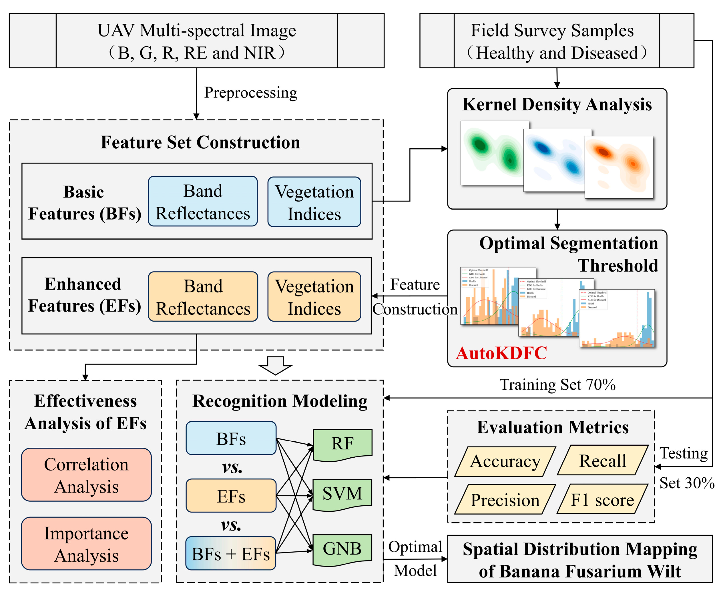
2. Materials and Methods

2.1. Study Area and Data
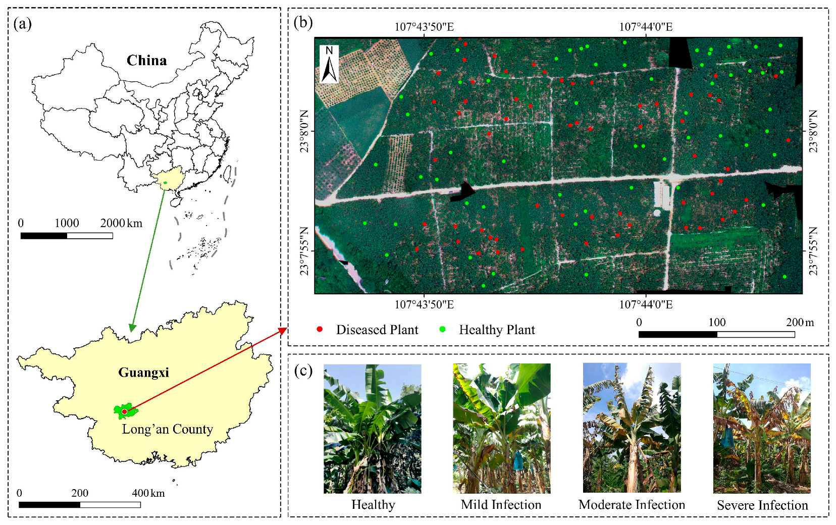
2.1.1. Study Area

The study area is in Long’an County, Nanning City, Guangxi Zhuang Autonomous Region, China (23°7′53.2″–23°8′4.0″ N, 107°43′44.9″–107°44′7.2″ E) (Figure 1a). Characterized by a subtropical monsoon climate, the region enjoys abundant sunlight and rainfall, with an average annual temperature ranging from 20.8 °C to 22.4 °C and an average annual precipitation of approximately 1200 mm—conditions highly favorable for banana cultivation. Bananas from Long’an County are known for their high quality and have gained considerable recognition in the national market. As of 2022, the total banana cultivation area in the county reached approximately 7840 hectares, with an annual output of 300,000 tons.
The specific study site is a banana plantation located about 5 km southeast of Long’an County’s urban center, covering an area of approximately 21 hectares (Figure 1b). The plantation grows the “Williams B6” variety, with the plants reaching a height of approximately 2.4 to 3 m and bearing 34 to 36 leaves. The planting density is about 1950 plants per hectare, with a spacing of 2.0 m × 2.6 m, and the growth period spans 10 to 12 months. A field survey conducted in August 2018 revealed severe BFW occurrence in this plantation, with over 40% of the plants exhibiting symptoms of varying severity (Figure 1c).

2.1.2. Data and Preprocessing

Field Survey of Banana Fusarium Wilt
On 7 August 2018, the research team conducted a field survey in Long’an County, Guangxi. A total of 120 samples were evenly collected across the study area to assess the occurrence of BFW, with each sample corresponding to a single banana plant (Figure 1b). BFW recognition was based on the proportion of yellowing leaf area relative to the total leaf area of the plant. Plants with less than 1% yellowing were classified as healthy, while those exceeding this threshold were considered diseased. During the field survey, we obtained the latitude and longitude of each sampled plant using a high-precision handheld GPS device and recorded its infection status (healthy or diseased). Ultimately, 57 healthy samples and 63 diseased samples were obtained and used for model training and validation.
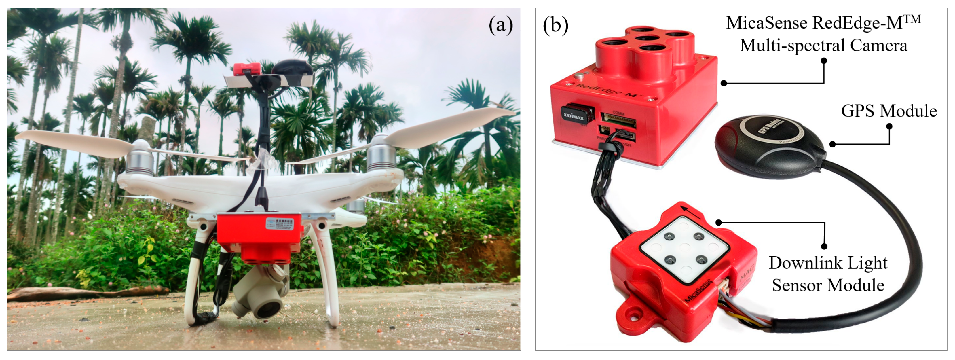
UAV Multi-Spectral Data Acquisition and Preprocessing
Multi-spectral data of the banana plantation were collected using a DJI Phantom 4 UAV (Shenzhen Dajiang Innovation Technology Co., Ltd., Shenzhen, China) equipped with a MicaSense RedEdge-M™ multi-spectral imaging system (Figure 2), manufactured by MicaSense, Inc., Seattle, WA, USA. The imaging system, which was mounted on the drone by a professional UAV developer, consists of a MicaSense RedEdge-M™ multi-spectral camera with a downlink light sensor (DLS) module and a GPS module, acquiring data across five spectral bands: blue, green, red, red edge, and near-infrared. The camera uses an external power supply with a voltage range of 4.2 V DC to 15.6 V DC, power consumption of 4 W, and peak power of 8 W. With these loads, the UAV can fly for at least 20 min under ideal conditions. All the spectral data were recorded as geotagged TIFF files and stored onboard the camera’s memory card.
Aerial imaging was conducted between 12:30 and 13:30 on 7 August 2018, under a clear sky and low wind conditions. When collecting data, the UAV flew at an altitude of 120 m above ground level, and the flight plan ensured cross-track and along-track overlap of 80%. The acquired multi-spectral imagery by the UAV covered an area of 21 hectares. The ground sampling resolution was 8 cm/pixel. Prior to and following the flight, images of the MicaSense calibrated reflectance panel were captured using the RedEdge sensor, manufactured by MicaSense, Inc., Seattle, WA, USA. The Pix4D mapper V4.5.6 software was used to process the images. These calibration images were used to perform radiometric correction of the UAV imagery, converting raw digital number values into reflectance data.
To integrate the ground-surveyed samples and UAV imagery, the sample data layer was overlaid with the UAV imagery layer in ArcGIS 10.6. The sample locations were manually adjusted to align with the centers of the corresponding banana plants in the UAV imagery, ensuring a precise match between the ground survey points and the plant centers in the UAV imagery. The processed data were stored in shapefile format. Subsequently, vector polygons were digitized for 120 banana plants, and the mean UAV-derived spectral reflectance and vegetation index values within each polygon were extracted for analysis.

2.2. Methods

Based on the UAV multi-spectral imagery and ground survey samples of BFW, this study first constructed basic features (BFs), including band reflectances (BRs) and vegetation indices (VIs). Subsequently, enhanced features (EFs) were generated using an automated kernel density segmentation method, which leverages differences in the kernel density distributions of healthy and diseased samples. These EFs were designed to amplify subtle spectral variations indicative of early-stage infection. Three ML algorithms were then employed to build recognition models of BFW, and the contribution and effectiveness of the EFs in improving the model performance were evaluated. Finally, the optimal model was used to generate a spatial distribution map of BFW in the study area. The methodological framework is illustrated in Figure 3.

2.2.1. Construction of Basic Features

Considering the remote sensing data source and this study’s objectives, BRs and VIs were selected as BFs. The band reflectance provides information on the canopy’s physiological condition; thus, the reflectance of five spectral bands—blue, green, red, red edge, and near-infrared—was included. Considering the physiological mechanisms of BFW—such as reductions in chlorophyll, carotenoids, and anthocyanins, leading to leaf yellowing, and impaired water transport, causing wilting and a decline in the leaf area index—eight VIs were also derived from these bands. These indices are sensitive to changes in plant pigments and structure caused by disease and include the following: Normalized Difference Vegetation Index (NDVI), Red Edge Normalized Difference Index (NDRE), Chlorophyll Index Green (CIgreen), Chlorophyll Index Red Edge (CIRE), Structure-Insensitive Pigment Index (SIPI), Red Edge Structure-Insensitive Pigment Index (SIPIRE), Carotenoid Reflectance Index (CARI), and Anthocyanin Reflectance Index (ARI). The formulas and corresponding physiological targets of these indices are presented in Table 1. In total, 13 BFs were constructed, comprising five BR-based BFs and eight VI-based BFs.
The specific feature extraction process was as follows. Based on the coordinates of the ground-surveyed banana Fusarium wilt samples and UAV multi-spectral imagery, the corresponding banana plants were located within the images. Using ArcGIS 10.6, vector outlines were drawn for 120 individual banana plants. Subsequently, eight vegetation indices were calculated from the UAV-acquired multi-spectral images. For each banana plant, the mean values of the reflectance across five spectral bands and the eight vegetation indices within its corresponding contour area were extracted as the sample’s feature values. In total, 13 basic features were obtained for each of the 120 samples, and the data were compiled into a CSV file.

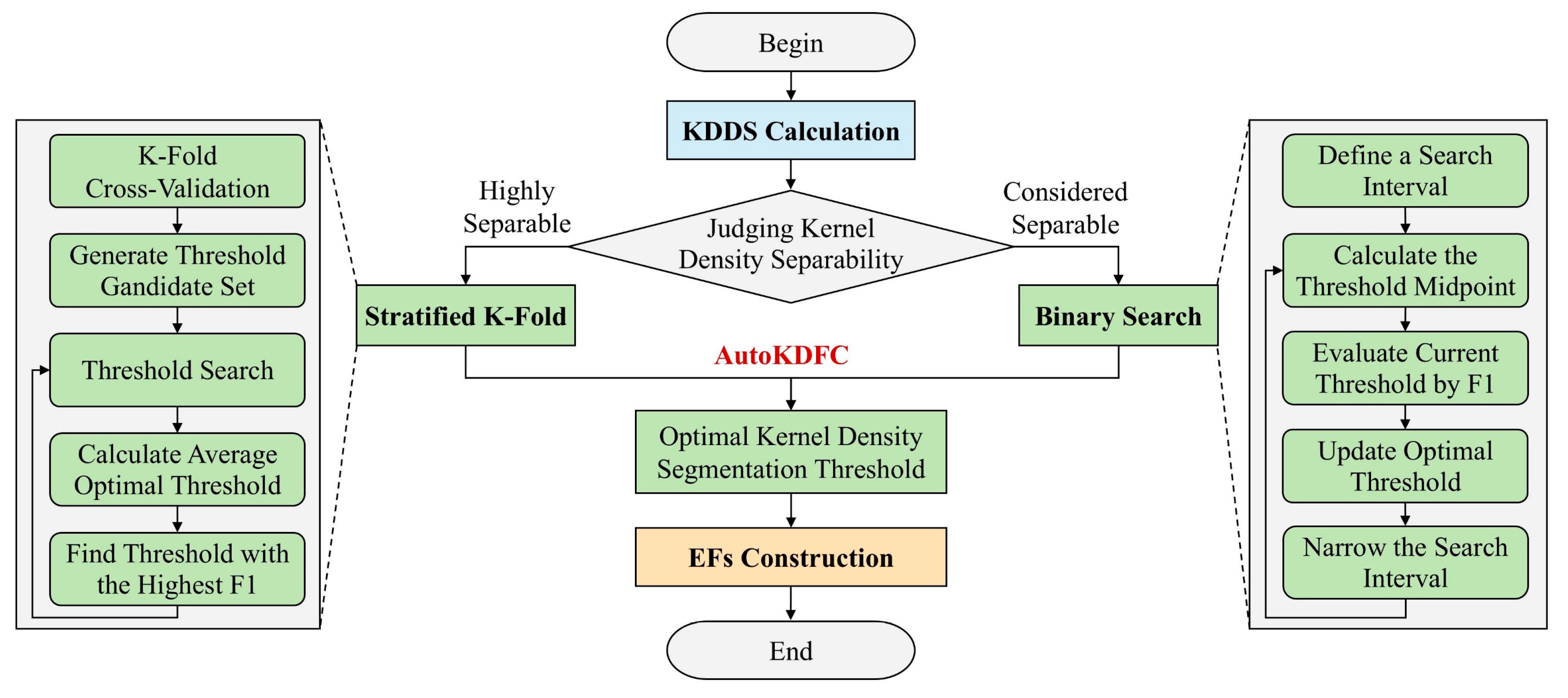
2.2.2. Automated Construction of Enhanced Features

The EFs developed in this study aim to capture subtle spectral variations associated with early disease onset, thereby improving the predictive performance of BFW recognition models. By analyzing the distributional differences of the BR-based BFs and VI-based BFs between healthy and diseased samples, optimal segmentation thresholds were identified, and the BFs were discretized into binary values. This transformation reduces the noise sensitivity and enhances the detectability of weak spectral signals. Kernel density estimation (KDE), a non-parametric method for estimating probability density functions, was employed to reveal the structure of the feature distributions [36]. Accordingly, this study proposed an automated kernel density segmentation-based feature construction algorithm (AutoKDFC), which includes the following steps: (1) define a discriminant metric to assess the separability of each BF; (2) determine the optimal threshold for feature segmentation; and (3) generate binary EFs based on the optimal threshold. The algorithm workflow is shown in Figure 4.
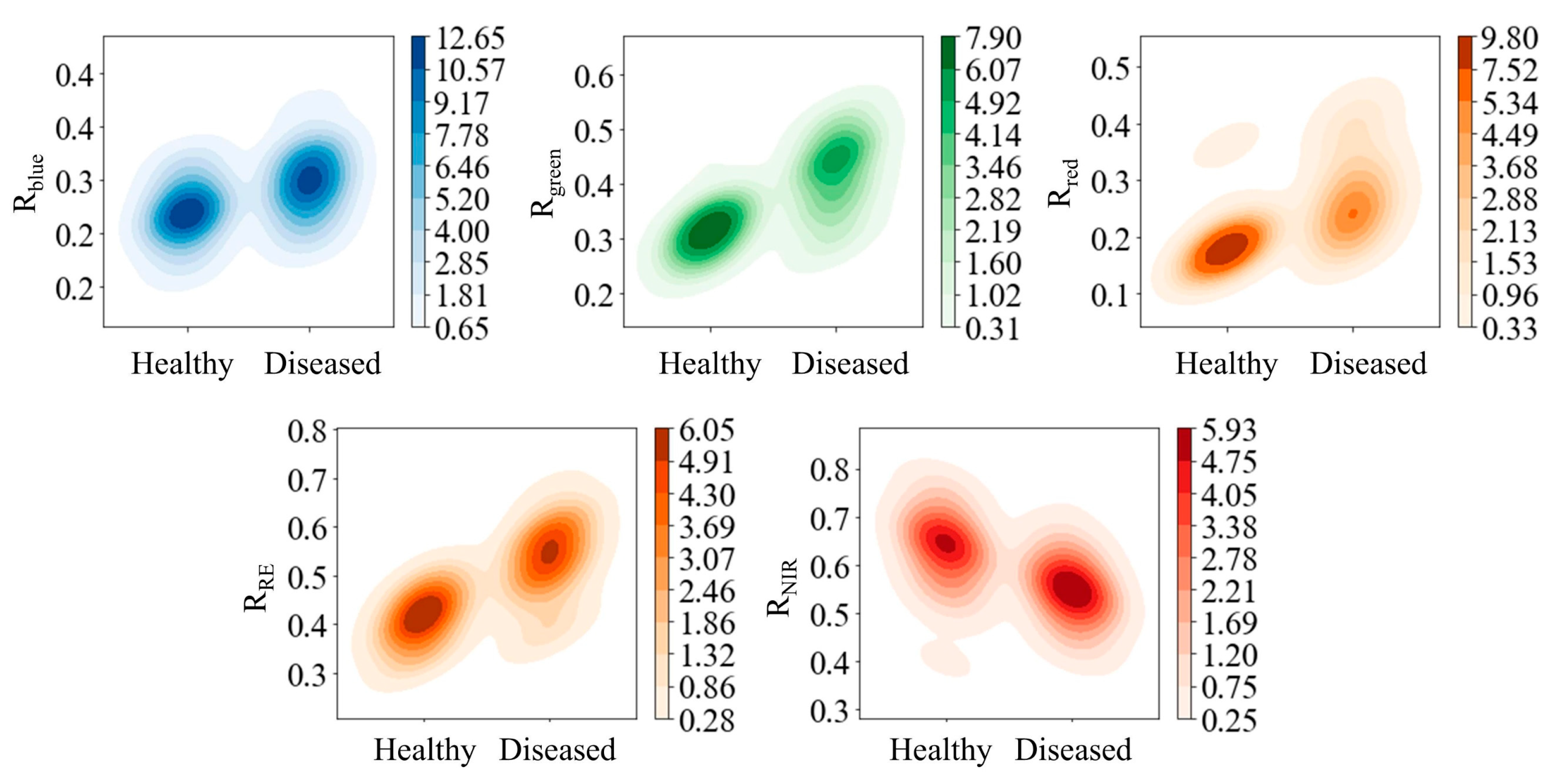
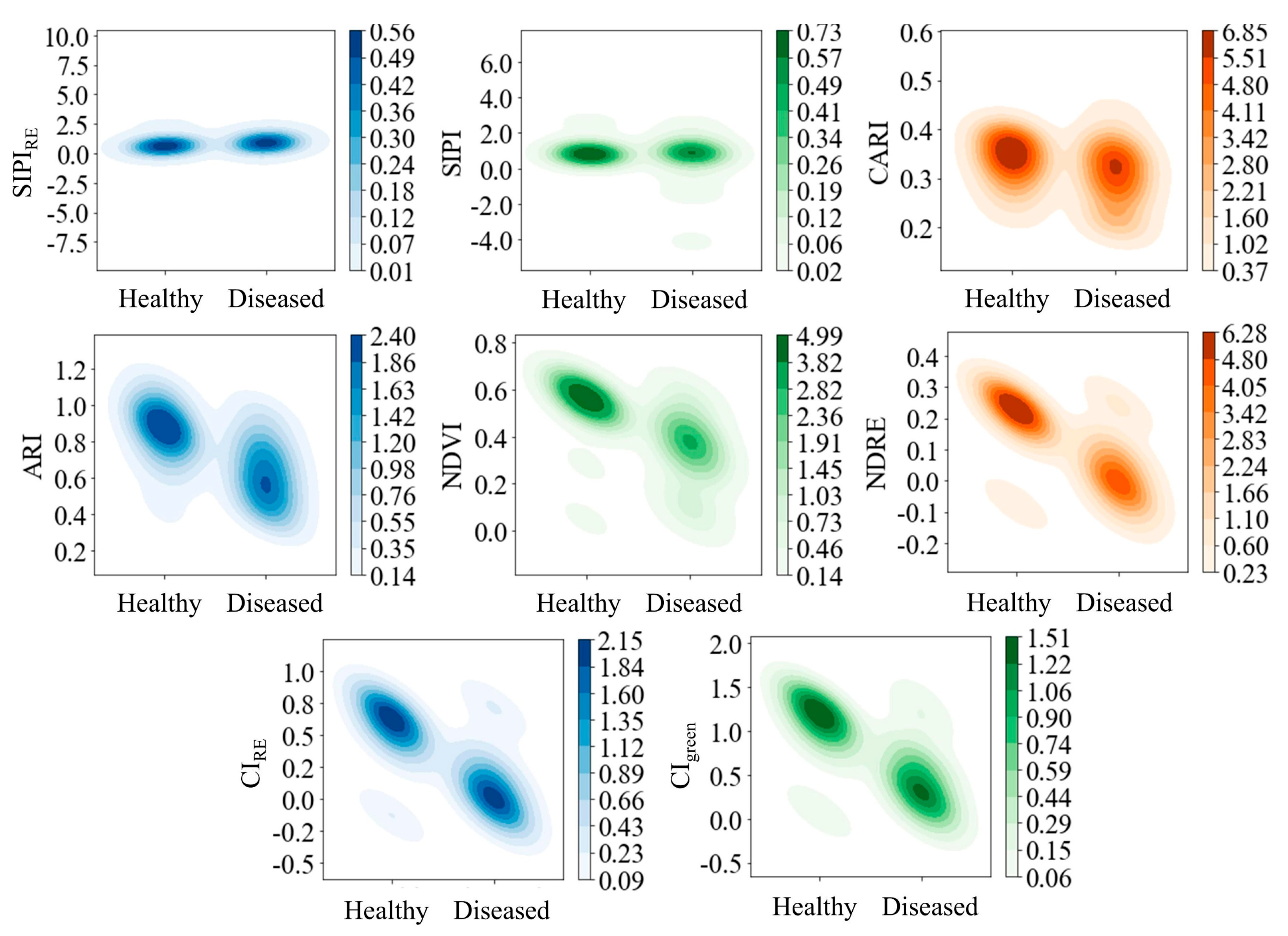
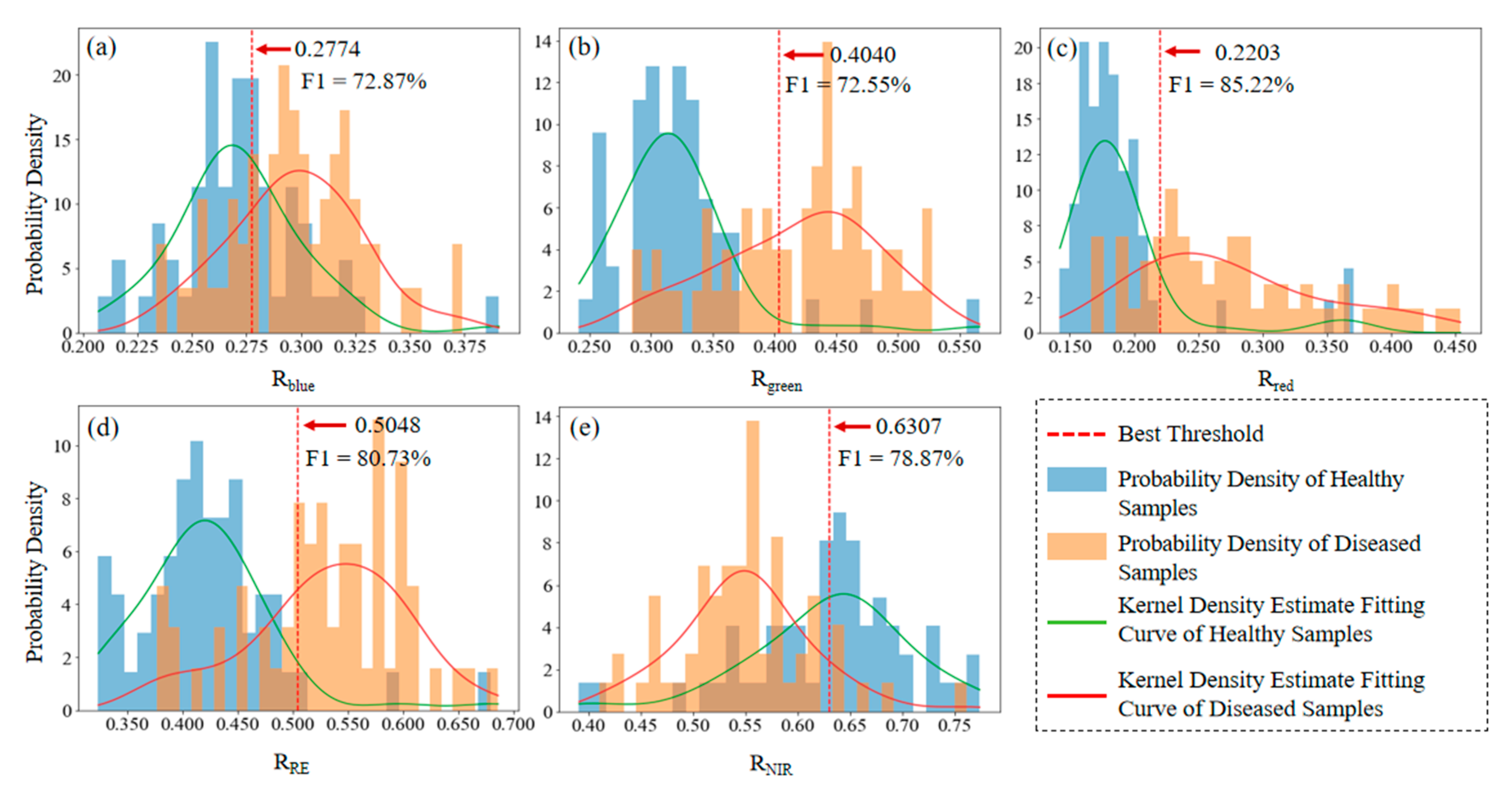
Evaluation of Basic Feature Separability Using Kernel Density
Figure 5 and Figure 6 illustrate the kernel density distributions of the BRs and VIs for healthy and diseased plants. Except for SIPIRE and SIPI, most features showed notable differences in the kernel density distributions between the two classes, indicating their potential for disease discrimination. However, there were considerable differences in the sensitivity of these features to BFW, as observed in the kernel density magnitudes, distribution shapes, and isodensity contour characteristics. These variations impact the selection of optimal thresholds and necessitate a quantitative evaluation of feature separability. To this end, this study developed a separability metric—the Kernel Density Discriminant Score (KDDS)—to quantify the separability of each basic feature. The features were then categorized into three levels: non-separable, considered separable, and highly separable, forming the basis for the subsequent threshold determination and EF construction.
We propose that the greater the vertical distance between the kernel density distributions of healthy and diseased samples, the lower the overall data dispersion and the lesser the overlap of isodensity contours, thereby indicating stronger feature separability. Accordingly, the Kernel Density Discriminant Score (KDDS) was defined as follows:
K D D S = d i s t s t d t o t a l + r a t i o = arg max f h x x arg max f d x x 1 n i = 1 n x i μ h 2 + 1 m i = 1 m x i μ d 2 + n max n t o t a l
where d i s t represents the distance between the “kernels” (the contour lines corresponding to the kernel density peaks) of the healthy and diseased samples in the vertical direction. The larger the value, the stronger the separability of the feature. The values of arg max f h x x and arg max f d x x represent the feature values corresponding to the kernel density peaks of healthy and diseased samples, respectively. s t d t o t a l is the sum of the standard deviations of the healthy and diseased samples, representing the overall dispersion (i.e., distribution width) of the two classes of sample data. The smaller the value, the stronger the separability of the feature. n and m represent the number of healthy and diseased samples, respectively, while μ h and μ d are their means. ratio represents the non-overlap rate of the contour lines, with a higher value indicating the stronger separability of the feature. n m a x is the larger number of non-overlapping contour lines between healthy and diseased samples, while n t o t a l is the total number of contour lines. In this study, the number of contour lines for healthy and diseased samples is set to be the same.
Once the KDDS values for all BFs are computed, they were categorized into three levels: non-separable, considered separable, and highly separable. Given that the KDDS values range from [0, +∞), a stepwise median method was employed to define the separability thresholds (Figure 7). Specifically, the KDDS values were sorted in ascending order. Features with KDDS values below the second median (Median 2) were labeled as non-separable; those between Median 2 and Median 3 were considered separable; and values above Median 3 were deemed highly separable. The first median (Median 1) was used solely to assist in computing Medians 2 and 3.
Using this approach, the separability levels were determined for all 13 BFs (Figure 8). The features SIPIRE, SIPI, and CARI were deemed non-separable and therefore unsuitable for EF construction. In contrast, RNIR, Rblue, Rgreen, Rred, and RRE were classified as considered separable, and ARI, NDVI, NDRE, CIRE, and CIgreen as highly separable, indicating that 10 EFs could be constructed.
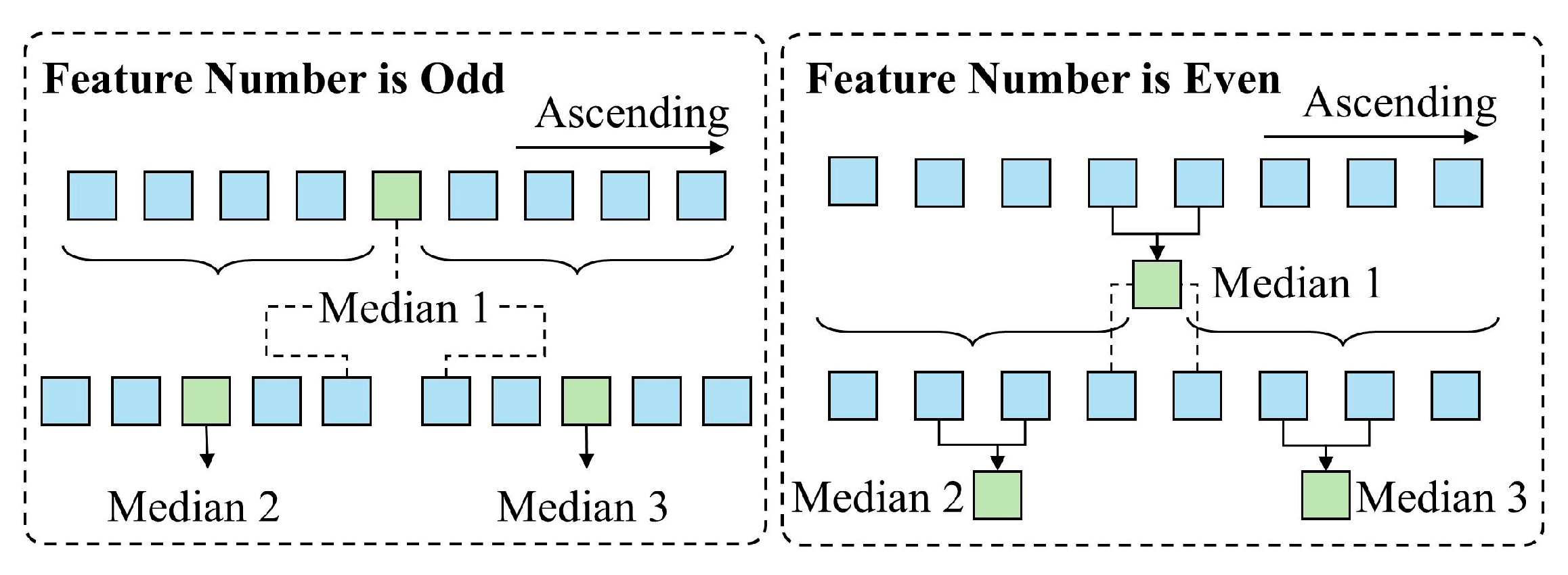
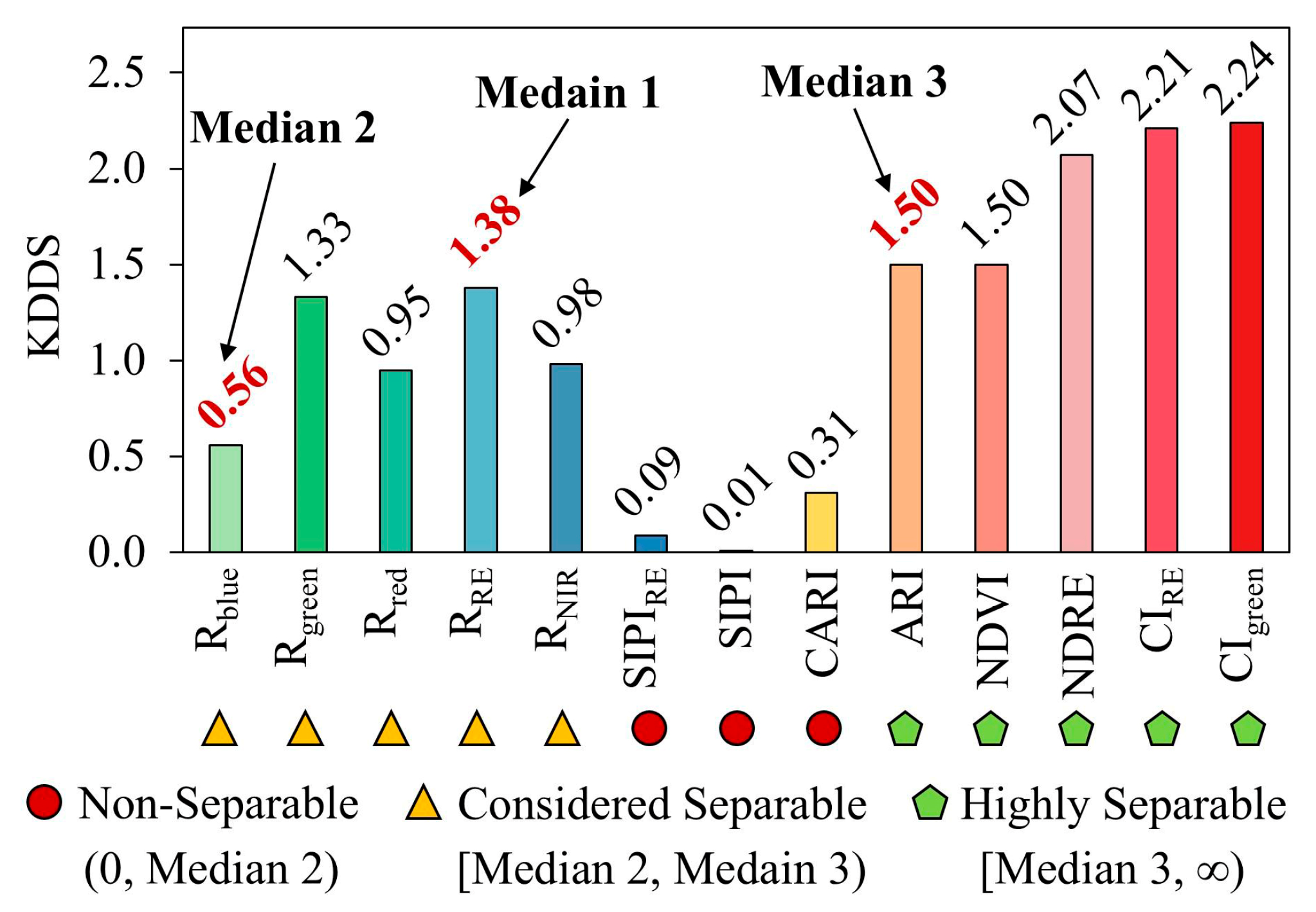
Automatic Determination of Optimal Segmentation Thresholds
The AutoKDFC employs two distinct strategies to determine the optimal segmentation threshold (OST) for the considered separable and highly separable features.
(1)
Highly Separable Features—Stratified K-Fold Cross-Validation
In cases where a feature is highly separable, the distributions of healthy and diseased samples differ significantly, and the model performance is relatively insensitive to the specific threshold. However, relying on a single dataset can introduce randomness and reduce robustness. To address this, we apply stratified K-fold cross-validation (K = 5) to evaluate the F1 score across multiple train–validation splits and select the threshold with the best generalization performance. The procedure is as follows:
  • Uniformly sample candidate thresholds within the range from the minimum to maximum values of the basic feature (e.g., NDVI) in the training set.
  • For each threshold, label samples based on whether the NDVI value is below or above the threshold (label 0 or 1, respectively).
  • Compute the F1 score on the validation set for each threshold.
  • Identify the threshold with the highest F1 score and record both the threshold and corresponding F1 score.
  • Compute the mean F1 score and the mean optimal threshold across all folds.
(2)
Considered Separable Features—Binary Search
For the considered separable features with overlapping distributions across healthy and diseased samples, precisely locating the threshold is critical. As the optimal thresholds for these features tend to lie within a narrow interval, binary search provides an efficient way to narrow the search space and approach the optimal threshold. This study employs binary search based on the F1 score as the evaluation metric. The procedure is as follows:
  • Set the minimum and maximum values of the feature (e.g., Rblue) as the initial search interval.
  • In each iteration, compute the midpoint as a candidate threshold and evaluate its F1 score.
  • If the current F1 score exceeds the previous best, update the optimal threshold.
  • Adjust the search interval based on the F1 score: If the left interval yields a better F1 score, narrow the search interval to the left (update Rblue_max); otherwise, narrow the search interval to the right (update Rblue_min).
  • Terminate the search when the range is less than 1 × 10⁻⁵ or the maximum number of iterations (max_iter) is reached, and return the optimal threshold and its F1 score.
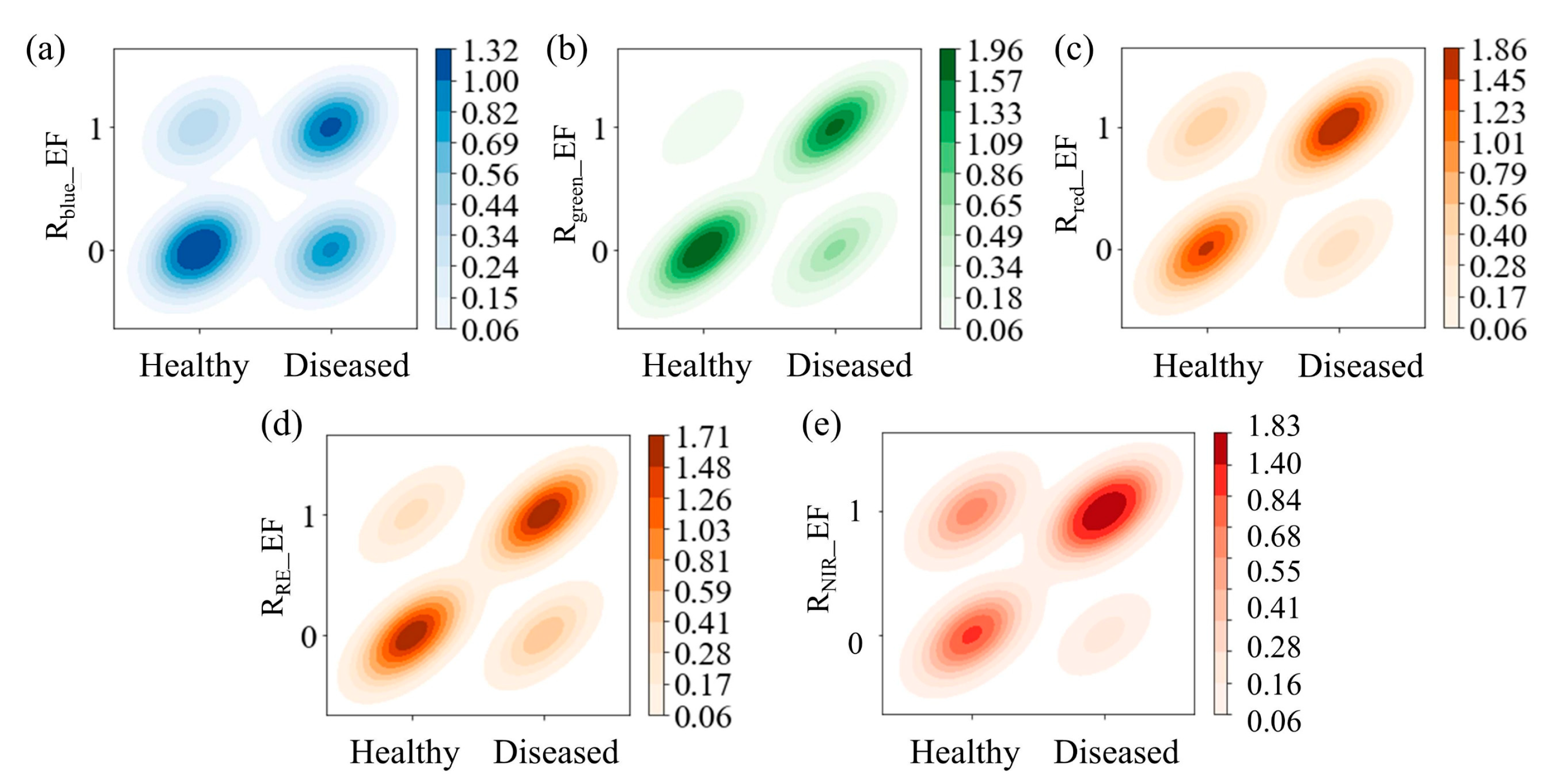
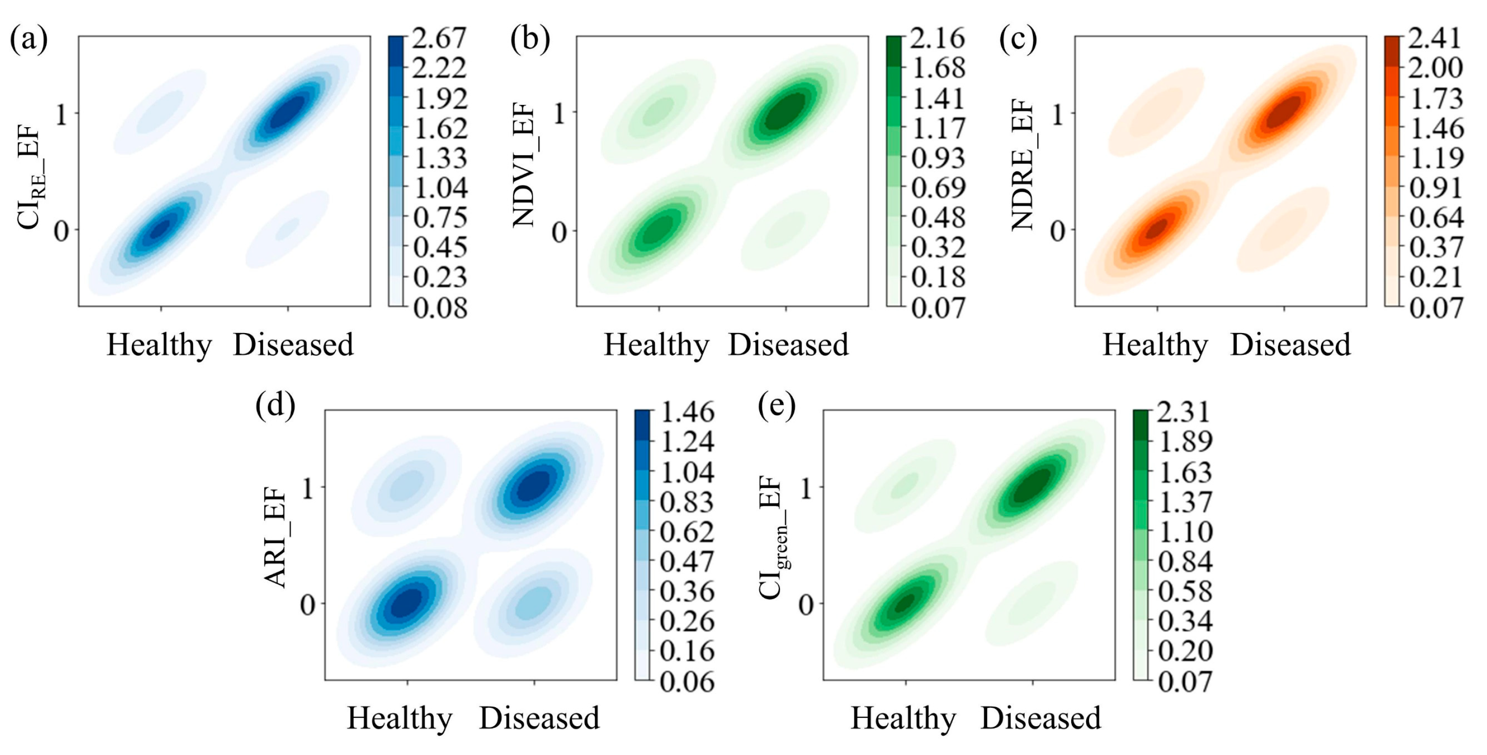
Construction of Enhanced Features Based on OST
After determining the OST for each BF, EFs are constructed by comparing the feature values corresponding to the kernel density peaks of healthy and diseased samples (denoted as Hvalue and Dvalue, respectively). The strategy is as follows. If the Hvalue of a BF > Dvalue, construct the EF using Equation (2); if the Hvalue of a BF < Dvalue, build the EF according to Equation (3).
EF i = 1 ,   i f   B F i < O S T i   0 ,   e l s e  
EF i = 0 ,   i f   B F i     O S T i 1 ,   e l s e  
where EFi represents the enhanced feature i, BFi represents the basic feature i, and OSTi represents the optimal segmentation threshold for BFi, where, i = 1, 2, …, 10, referring to the ten BFs selected for enhancement.
Ultimately, 10 EFs are constructed from the 13 BFs, increasing the total number of features to 23, as detailed in Table 2.

2.2.3. Machine Learning Modeling

(1) Machine Learning Algorithms
Three ML algorithms were employed in this study for the recognition task: random forest (RF), a decision-tree-based ensemble method; support vector machine (SVM), a kernel-based approach; and Gaussian naive Bayes (GNB), a probabilistic model. The dataset was randomly divided into a training set (70%: 84 samples) and a testing set (30%: 36 banana samples). The characteristics of each algorithm are as follows.
RF constructs an ensemble of decision trees using the bagging strategy, where each tree is built on randomly selected samples and feature subsets [37]. Its robustness against high-dimensional data, nonlinear relationships, and noisy inputs makes it particularly suitable for modeling field-collected banana data that may contain measurement errors. SVM identifies the optimal hyperplane that maximizes the margin between two classes based on statistical learning theory [38]. Since the goal is binary classification—differentiating diseased from healthy banana plants—SVM is a suitable choice. It may even outperform RF in terms of generalization, especially when dealing with small datasets. GNB assumes that features follow a Gaussian distribution and applies Bayes’ theorem under the assumption of conditional independence among features [39]. As the dataset includes multiple continuous BR-based BFs and VI-based BFs, GNB provides an effective way to model such continuous inputs.
(2) Experimental Setup for BFW Recognition Modeling
To evaluate the effectiveness of EFs in improving model performance, two sets of comparative experiments and four model configurations were designed for BFW recognition. These configurations primarily differ in their feature set, as shown in Table 3 (Models I–IV). The comparison between Model I and Model II was intended to test whether the inclusion of EFs improves the recognition performance. The comparison between Model III and Model IV aimed to determine whether EFs outperform BFs in identifying BFW.
In this study, the experiments were conducted in a local Anaconda environment using Jupyter Notebook 6.3.0. The experimental setup included the Windows 10 operating system and the Python 3.8.8 interpreter. For reproducibility, the random_state parameter was set to 42 for both RF and SVM. All the other parameters were kept at their default settings. The implementations used were as follows: RF, sklearn.ensemble.RandomForestClassifier; SVM, sklearn.svm.SVC; GNB, sklearn.naive_bayes.GaussianNB.

2.2.4. Model Performance Evaluation

The performance of the BFW recognition models was evaluated using four metrics: accuracy, precision, recall, and F1 score (Equations (4)–(7)). Accuracy measures the overall correctness of the model’s predictions. Precision assesses the proportion of true positive predictions among all the positive predictions, reflecting the model’s ability to avoid false positives. Recall evaluates the proportion of true positives that were correctly identified, reflecting the model’s ability to detect actual positives. F1 score is the harmonic mean of the precision and recall, providing a balanced evaluation of both aspects. All the metrics range from 0 to 1, with higher values indicating better model performance. To ensure fairness and robustness in the evaluation, the train–test split (70% training, 30% testing) was repeated 50 times with random sampling. The arithmetic mean of the performance metrics across these runs was reported as the final score.
A c c u r a c y = T P + T N T P + T N + F P + F N
P r e c i s i o n = T P T P + F P
R e c a l l = T P T P + F N
F 1   S c o r e = 2 P r e c i s i o n R e c a l l P r e c i s i o n + R e c l a l
where TP denotes the number of samples predicted as healthy that are indeed healthy, FP represents the number of samples predicted as healthy but actually diseased, FN refers to the number of samples predicted as diseased but actually healthy, and TN indicates the number of samples predicted as diseased that are indeed diseased.

3. Results

3.1. Optimal Kernel Density Segmentation Thresholds

Figure 9 and Figure 10 present the optimal kernel density segmentation thresholds and corresponding F1 scores obtained using the AutoKDFC for five BR-based BFs and five VI-based BFs. The results show that among the five BRs, Rblue, Rgreen, and RNIR exhibited relatively weak performance, with F1 scores ranging from 72% to 78%, while Rred and RRE achieved better results, with F1 scores exceeding 80%. The VIs outperformed the RF features overall, with all the F1 scores above 90% except for ARI, which scored 84.36%, indicating the high reliability of the automatically derived thresholds. The kernel density distributions for healthy and diseased samples show significant overlaps for Rblue, Rgreen, RNIR, and ARI, which likely explains their lower thresholding performance (further discussed in the Section 4). Overall, the optimal segmentation thresholds of the VIs were superior, suggesting that VI-based EFs are more effective than BR-based EFs in distinguishing the health status of banana plants affected by BFW.

3.2. Effectiveness of Enhanced Features

To assess the effectiveness of the constructed EFs in terms of BFW recognition, this study analyzed their correlation with plant health status and their relative importance.

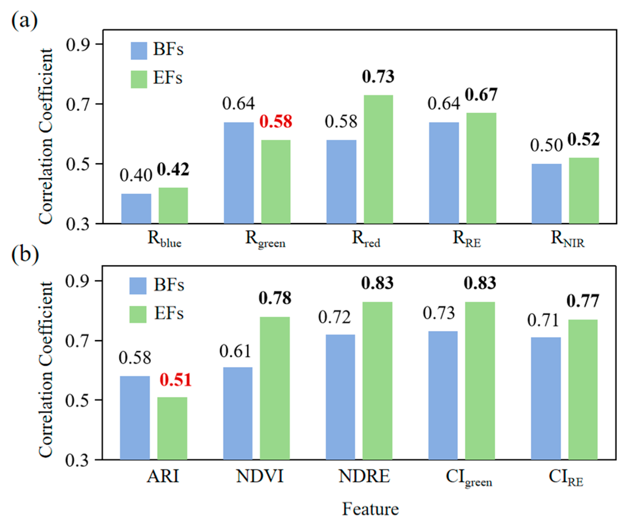
3.2.1. Correlation Analysis

Figure 11 and Figure 12 show the kernel density distributions of the EFs for healthy and diseased plants. Compared to the BFs, the EFs demonstrate more pronounced distributional differences between healthy and diseased plants. Their kernel density curves are more uniform and show greater separability, highlighting their stronger discriminative capacity for BFW recognition. Additionally, a comparison between Figure 10 and Figure 11 reveals that the VI-based EFs exhibit better class separability and more consistent distribution patterns than the BR-based EFs.
Pearson correlation coefficients were used to analyze the correlation between the EFs/BFs and the BFW severity (Figure 13). Figure 13a indicates that, except for Rgreen, all the BR-based EFs show higher correlations with BFW than the BFs, with Rblue, Rred, RRE, and RNIR increasing by 2%, 15%, 3%, and 2%, respectively. Figure 13b shows that although ARI’s correlation dropped by 7%, NDVI, NDRE, CIgreen, and CIRE improved by 17%, 11%, 10%, and 6%, respectively. In general, most EFs constructed by the AutoKDFC improved the correlation with BFW, thereby enhancing the separability of healthy and diseased plants. The reduced correlation of Rgreen and ARI may be attributed to the poor segmentation thresholds (as discussed in Section 3.1) and low sensitivity of the Rgreen band to BFW (further explored in the Section 4.1).

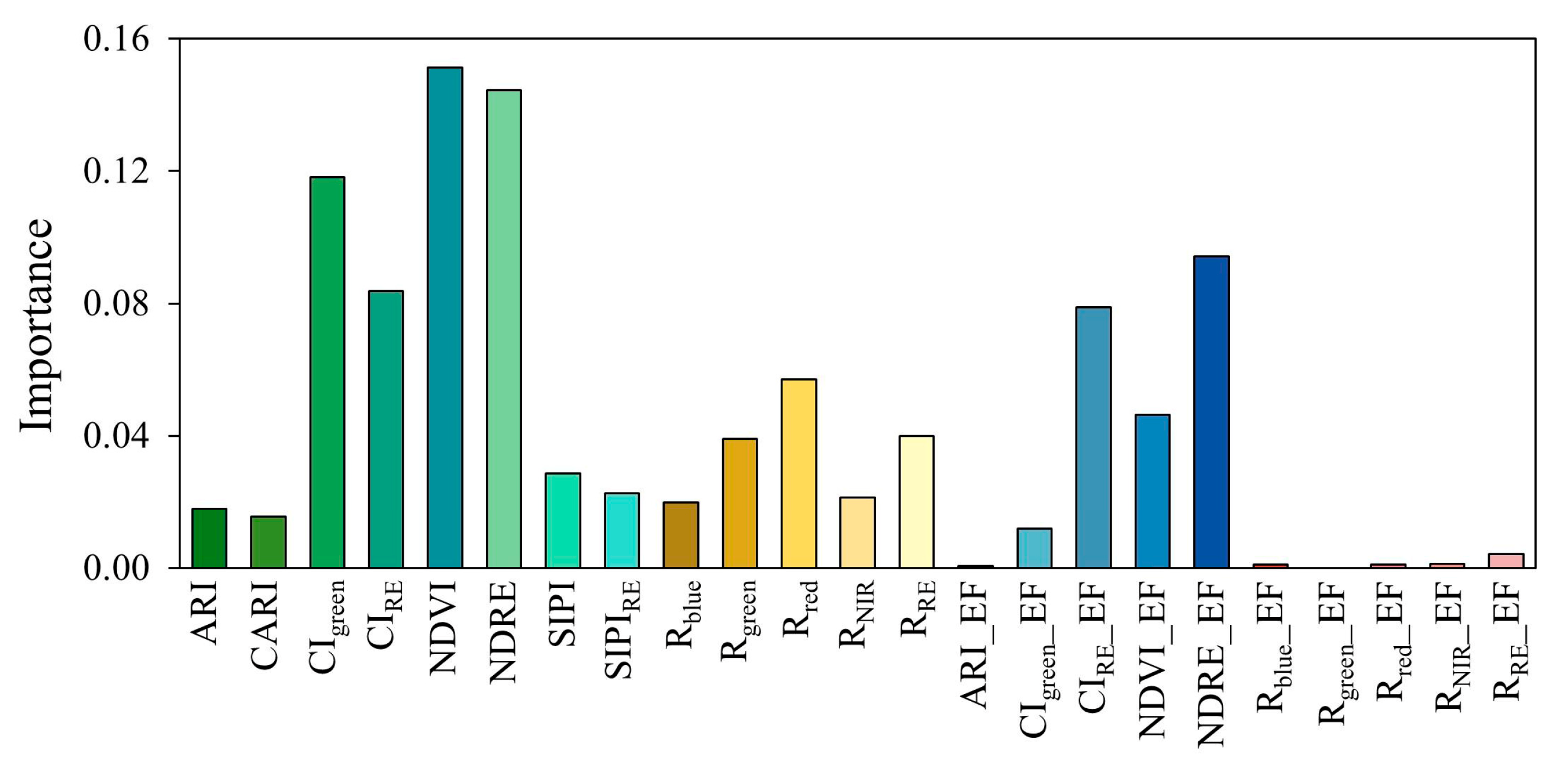
3.2.2. Feature Importance Analysis

Since the SVM and GNB algorithms cannot directly quantify feature importance, the built-in feature importance function of the RF algorithm was used for analysis. Figure 14 displays the relative importance of all 23 features. The results indicate that, apart from ARI_EF, the VI-based EFs generally hold higher importance, with some even exceeding that of BR-based BFs. Among the BR-based EFs, only RRE_EF showed notable importance, while the others were comparatively low. Overall, the EFs constructed using the AutoKDFC were found to be highly relevant in terms of BFW recognition, with the VI-based EFs demonstrating greater significance than the BR-based ones. Possible reasons why certain EFs performed worse than their basic counterparts will be explored further in Section 4.

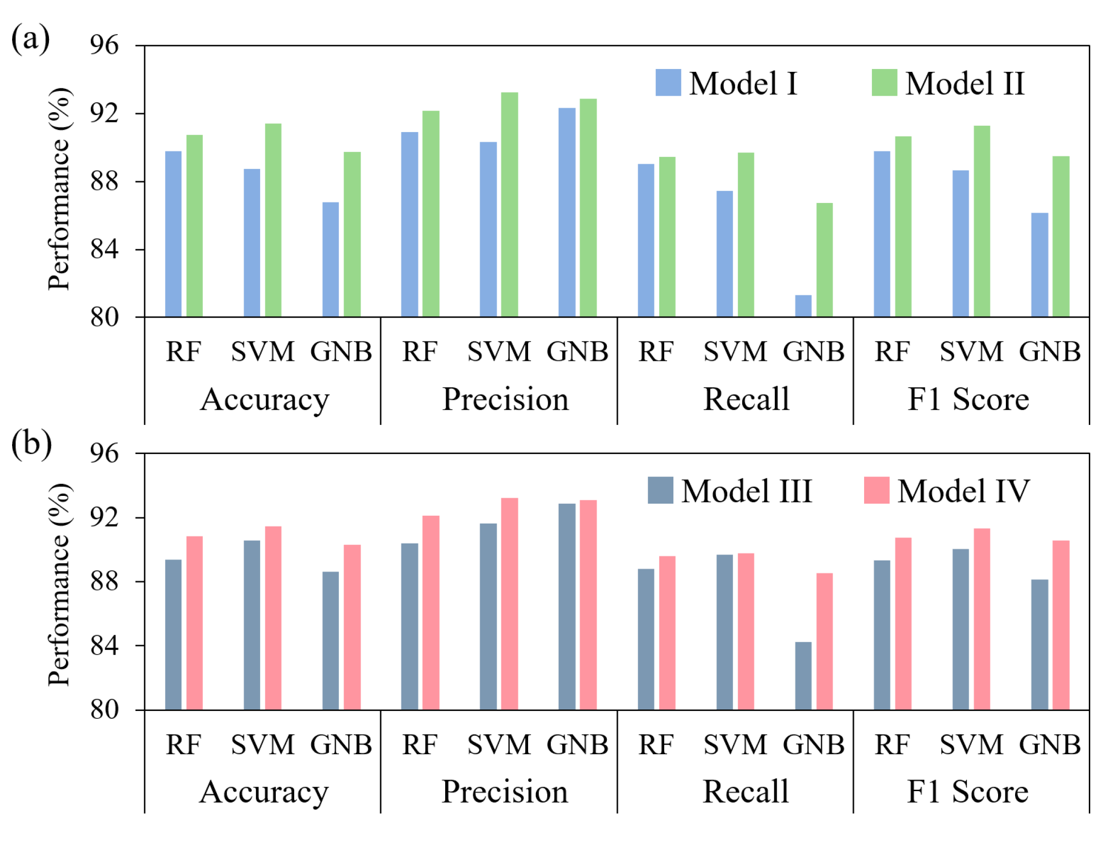
3.3. Predictive Performance of BFW Recognition Models

Figure 15 and Table 4 provide both visual and quantitative comparisons of the model performance from two sets of experiments: Experiment 1 (Model I vs. Model II, using 13 BFs vs. 23 EFs) and Experiment 2 (Model III vs. Model IV, using 10 BFs vs. 10 EFs). In Experiment 1, both Figure 15a and Table 4 show improvements in all the performance metrics across the algorithms when the EFs were added, with the greatest average improvement observed in GNB (3.07%) and the smallest in RF (0.88%). Before introducing the EFs, RF was the best-performing model, whereas after enhancement, SVM achieved the highest accuracy at 91.39%. In Experiment 2, as shown in Figure 15b and Table 4, models using only the EFs outperformed those using only BFs across all three algorithms, again confirming the superior discriminative ability of the EFs. SVM continued to perform best, with an average accuracy of 91.44%. Overall, the EFs significantly improved the model prediction performance and demonstrated strong adaptability across multiple algorithms, with the most substantial improvement observed in SVM. This may be attributed to the consistency between SVM’s optimal hyperplane classification principle and the design rationale behind the EFs.
Additionally, despite having fewer features, Models III and IV outperformed Models I and II, which had more features. This suggests that combining BFs and EFs might introduce redundancy, potentially reducing the model generalizability. An increased number of features could lead the models to overfit noise in the data rather than learn meaningful distinctions, ultimately affecting the test set performance. Therefore, future studies should consider optimized combinations of BFs and EFs to balance their contributions and improve the model accuracy and generalization under varying conditions.

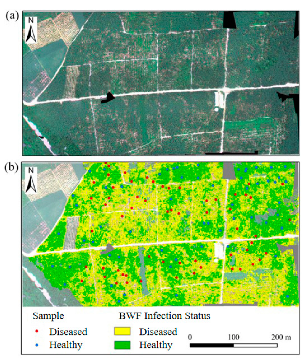
3.4. Spatial Distribution Mapping of Banana Fusarium Wilt

Given that SVM was identified as the optimal-performing model, it was selected for mapping the spatial distribution of BFW. Although Model IV (EFs only) achieved the highest accuracy, completely replacing the BFs could risk information loss or reduced feature stability, as the EFs are derived from the basic ones. Thus, Model II, which integrates both BFs and EFs and achieved only a marginally lower accuracy (by 0.05%), was ultimately chosen for the mapping task.
In the mapping process, banana planting areas in the study region were first extracted using texture features and the NDVI. Then, the SVM model based on Model II was applied to predict the spatial distribution of BFW (Figure 16). The results show that the red dots (diseased samples) in Figure 15 are primarily located within the yellow regions (predicted diseased plants), while the blue dots (healthy samples) align well with the green regions (predicted healthy plants), indicating strong agreement between the model predictions and the actual conditions. Furthermore, the spatial pattern of the yellow areas in Figure 16b closely matches the distribution of bare soil zones shown in Figure 16a. This is likely because banana plants infected with BFW exhibit drooping and withered leaves, reducing canopy coverage and increasing soil exposure, which in turn alters the spectral characteristics. This observed phenomenon further supports the validity of the model’s predictions.

4. Discussion

4.1. Mechanistic Interpretation of Feature Separability and Threshold Rationality

The separability of the kernel density distributions for a given feature primarily depends on its sensitivity to BFW—specifically, the distributional differences between healthy and diseased samples. Upon infection, the pigment content of banana leaves changes significantly during disease progression, with leaves turning from green to yellow and eventually withering to a grayish–white color. These pigment alterations result in shifts in the spectral reflectance, with varying magnitudes across different bands. As the chlorophyll content decreases, the reflectance in the Rred and RNIR bands increases, while RRE decreases. Similarly, Rblue and Rgreen also increase, but to a lesser extent than Rred and RNIR [40,41]. Accordingly, all five BR-based BFs examined in this study showed a degree of separability, but Rblue and Rgreen performed poorly in threshold segmentation (F1 scores of 72.87% and 72.55%, respectively), with Rgreen being the weakest. Prior studies have shown that the reflectance in the green band is relatively stable under physiological stress, making it less effective for distinguishing between healthy and diseased vegetation [16]. This aligns with the current study, where the kernel density distributions of Rgreen show considerable overlap between healthy and diseased samples.
For the VI-based BFs, significant differences were observed between healthy and diseased samples in indices that reflect the chlorophyll content and leaf area index (e.g., NDVI, NDRE, CIgreen, and CIRE), resulting in high kernel density separability and rational threshold partitioning. In contrast, the carotenoid content remains relatively stable during early leaf yellowing, degrading only in the late stages of BFW when leaves turn brown or gray–white. Since no severely diseased (gray–white) samples were collected during the field surveys in this study, the kernel density distributions of SIPI, SIPIRE, and CARI—indices related to the carotenoid content—were similar between healthy and diseased samples, resulting in lower separability. Regarding the ARI index, which reflects the anthocyanin content, there is minimal change during the early infection stages, with anthocyanin gradually accumulating in the mid-to-late stages. As a result, diseased samples exhibit a dispersed kernel density distribution that overlaps with healthy samples, yielding a KDDS score near the threshold between “considered separable” and “highly separable” (median = 3), and leading to weaker threshold performance compared to other VIs.

4.2. Mechanistic Interpretation of the Importance of Enhanced Features

This study employed a nonlinear threshold-based transformation of BFs to construct EFs aimed to improving the recognition of spectral differences between healthy and diseased banana plants—especially for identifying subtle spectral vibrations during early infection stages. The model evaluation indicated that the inclusion or partial substitution with EFs improved the recognition of BFW. However, feature importance analysis using the RF algorithm (Figure 13) showed that EFs generally contributed less than their corresponding BFs. This phenomenon may stem from several factors. (1) Information redundancy: EFs are derived from BFs and, although optimized for disease recognition, share overlapping information sources. Consequently, in RF models, some EFs may be partially replaced by BFs, reducing their relative importance. (2) Feature discriminability: BFs capture global spectral differences between healthy and diseased plants, while EFs are tailored to optimize the discriminability in specific spectral ranges. Given that RF relies on multi-dimensional feature partitioning for classification, it tends to favor globally discriminative features, positioning EFs as supplementary. (3) Feature sensitivity differences: EFs may be more sensitive to subtle early-stage spectral vibrations, while in late stages—when spectral differences become more pronounced—BFs may play a dominant role, thereby diminishing the unique contribution of EFs.
In summary, while the inclusion of EFs improves disease recognition, their independent contribution is influenced by information redundancy, model preference, and disease progression, resulting in varying levels of impact across different models.

4.3. Methodological Benchmarking and Performance Reference to Similar Studies

In the field of plant disease recognition, model performance is highly dependent on the effectiveness of feature engineering. This study addresses the challenge of identifying BFW by innovatively proposing an enhanced feature construction method based on kernel density segmentation. A comparative analysis is presented below from two perspectives—feature engineering and model performance—against existing studies on BFW recognition.
In terms of feature engineering, compared with other BFW identification studies that rely solely on BFs [16,17], this study introduces EFs to improve the model’s ability to detect subtle spectral signals associated with early-stage BFW symptoms. Feature importance analysis shows that some EFs rank among the top five (Figure 14). In terms of model performance, compared with the logistic regression model using BFs in [16], which achieved an accuracy of 90.5%, the SVM model in this study reached an average accuracy of 91.39% through the use of EFs, demonstrating their effectiveness in boosting model performance. Although there are limitations in making direct comparisons across different plant diseases, the proposed enhanced feature construction approach may offer valuable insights for the monitoring of other crop diseases. Future work may apply this strategy to broader scenarios and conduct more extensive comparative studies.

4.4. Future Research Directions and Perspectives

This study validated the effectiveness of the AutoKDFC method for automatically constructing EFs in improving BFW recognition capability, offering a novel approach to plant health monitoring based on spectral features. However, several directions remain worthy of further exploration in future research:
(1)
Disease severity monitoring: EFs are constructed to capture subtle spectral vibrations during early-stage disease infection, showing particularly high recognition capability for mildly infected samples. However, due to the limited sample size, this study did not conduct an in-depth analysis of disease severity monitoring. Future research with a sufficient data volume could further validate the role of EFs in identifying mildly infected samples and evaluate their applicability across different disease progression stages.
(2)
Feature optimization: This study did not apply independent feature selection and instead combined BFs and EFs. Given their derivation, there may be significant information redundancy. Future work could apply feature selection methods such as the Pearson correlation coefficient [42], mutual information [43], or LASSO [44] to reduce redundancy and improve model generalizability [45,46,47].
(3)
Application extension: AutoKDFC demonstrates strong potential for disease recognition and could be extended to other crop disease monitoring tasks. Integrating this approach with multi-source remote sensing data and deep learning models may yield more efficient and accurate disease recognition systems, supporting the advancement of precision agriculture.

5. Conclusions

This study proposed the AutoKDFC to improve the spectral recognition of BFW. By applying threshold segmentation to basic features (BRs and VIs), the resulting EFs effectively captured subtle spectral vibrations in early infection stages. The experimental results showed that—except for a few vegetation indices—EFs based on VIs outperformed those based on BRs in BFW recognition. The inclusion of EFs significantly improved the recognition accuracy across multiple ML algorithms (RF, SVM, GNB), with SVM yielding the best overall performance. Although EFs ranked lower than BFs in importance within the RF model, their inclusion still notably improved the model performance, confirming their effectiveness in detecting early-stage spectral anomalies caused by BFW. Future work could further validate the ability of these features to detect mild disease cases through severity-stage monitoring. Additionally, combining BFs and EFs may introduce redundancy, and future efforts should focus on optimizing feature selection to enhance model generalizability. Overall, this study demonstrated the effectiveness and generalizability of the AutoKDFC method for BFW recognition and introduced a novel approach to spectral feature enhancement that could be applied to broader disease monitoring tasks, supporting precision agriculture and disease management.

Author Contributions

Conceptualization, Y.S., L.Z.; methodology, Y.S., H.Y.; software, Y.S.; validation, Y.S., H.L.; formal analysis, Y.S., L.Z., H.Y.; investigation, H.Y., W.K., B.Z.; resources, W.H., J.C.; writing—original draft preparation, Y.S., L.Z.; writing—review and editing, Y.S., L.Z., H.L., X.L., W.H., W.K., B.Z.; visualization, Y.S., L.Z.; supervision, J.C.; funding acquisition, L.Z., W.K., B.Z., J.C. All authors have read and agreed to the published version of the manuscript.

Funding

This research was funded by the National Natural Science Foundation of China (No. 42171323), the Hainan Provincial Natural Science Foundation of China (No. 623QN325, 322QN346), and the Research Foundation of Shenzhen Science and Technology Innovation Bureau (No. KCXFZ20240903093800002).

Data Availability Statement

The raw data supporting the conclusions of this article will be made available by the authors on request.

Conflicts of Interest

The authors declare no conflicts of interest.

References

  1. Shen, Z.; Xue, C.; Penton, C.R.; Thomashow, L.S.; Zhang, N.; Wang, B.; Ruan, Y.; Li, R.; Shen, Q. Suppression of banana Panama disease induced by soil microbiome reconstruction through an integrated agricultural strategy. Soil Biol. Biochem. 2019, 128, 164–174. [Google Scholar] [CrossRef]
  2. Ploetz, R.C. Fusarium Wilt of Banana. Phytopathology 2015, 105, 1512. [Google Scholar] [CrossRef] [PubMed]
  3. Ismaila, A.A.; Ahmad, K.; Siddique, Y.; Wahab, M.A.A.; Kutawa, A.B.; Abdullahi, A.; Zobir, S.A.M.; Abdu, A.; Abdullah, S.N.A. Fusarium wilt of banana: Current update and sustainable disease control using classical and essential oils approaches. Hortic. Plant J. 2023, 9, 1–28. [Google Scholar] [CrossRef]
  4. Pegg, K.G.; Coates, L.M.; O’Neill, W.T.; Turner, D.W. The Epidemiology of Fusarium Wilt of Banana. Front. Plant Sci. 2019, 10, 1395. [Google Scholar] [CrossRef]
  5. Ordonez, N.; Seidl, M.F.; Waalwijk, C.; Drenth, A.; Kilian, A.; Thomma, B.P.H.J.; Ploetz, R.C.; Kema, G.H.J. Worse Comes to Worst: Bananas and Panama Disease—When Plant and Pathogen Clones Meet. PLoS Pathog. 2015, 11, e1005197. [Google Scholar] [CrossRef]
  6. Segura-Mena, R.A.; Stoorvogel, J.J.; García-Bastidas, F.; Salacinas-Niez, M.; Kema, G.H.J.; Sandoval, J.A. Evaluating the potential of soil management to reduce the effect of Fusarium oxysporum f. sp. cubense in banana (Musa AAA). Eur. J. Plant Pathol. 2021, 160, 441–455. [Google Scholar] [CrossRef]
  7. Zhang, M.; Zhou, D.; Qi, D.; Wei, Y.; Chen, Y.; Feng, J.; Wang, W.; Xie, J. Research progress on the integrated control of Fusarium wilt disease in banana. Sci. Sin. Vitae 2024, 54, 1843–1852. [Google Scholar]
  8. Dita, M.; Barquero, M.; Heck, D.; Mizubuti, E.S.G.; Staver, C.P. Fusarium Wilt of Banana: Current Knowledge on Epidemiology and Research Needs Toward Sustainable Disease Management. Front. Plant Sci. 2018, 9, 1468. [Google Scholar] [CrossRef]
  9. Wang, W.; Liu, Z.; Zheng, C.; Zhang, L. Research Progress on Banana Fusarium Wilt. China Port Sci. Technol. 2024, 6, 44–51. [Google Scholar]
  10. Siamak, S.B.; Zheng, S. Banana Fusarium Wilt (Fusarium oxysporum f. sp. cubense) Control and Resistance, in the Context of Developing Wilt-resistant Bananas Within Sustainable Production Systems. Hortic. Plant J. 2018, 4, 208–218. [Google Scholar] [CrossRef]
  11. Lan, Y.; Zhu, Z.; Deng, X.; Lian, B.; Huang, Y.; Huang, Z.; Hu, J. Monitoring and classification of citrus Huanglongbing based on UAV hyperspectral remote sensing. Trans. Chin. Soc. Agric. Eng. 2019, 35, 92–100. [Google Scholar]
  12. Yu, R.; Luo, Y.; Zhou, Q.; Zhang, X.; Wu, D.; Ren, L. Early detection of pine wilt disease using deep learning algorithms and UAV-based multispectral imagery. For. Ecol. Manag. 2021, 497, 119493. [Google Scholar] [CrossRef]
  13. Liao, J.; Tao, W.; Zang, Y.; Wang, P.; Luo, X. Research Progress and Prospect of Key Technologies in Crop Disease and Insect Pest Monitoring. Trans. Chin. Soc. Agric. Mach. 2023, 54, 1–19. [Google Scholar]
  14. Duarte, A.; Borralho, N.; Cabral, P.; Caetano, M. Recent Advances in Forest Insect Pests and Diseases Monitoring Using UAV-Based Data: A Systematic Review. Forests 2022, 13, 911. [Google Scholar] [CrossRef]
  15. Kaivosoja, J.; Hautsalo, J.; Heikkinen, J.; Hiltunen, L.; Ruuttunen, P.; Näsi, R.; Niemeläinen, O.; Lemsalu, M.; Honkavaara, E.; Salonen, J. Reference Measurements in Developing UAV Systems for Detecting Pests, Weeds, and Diseases. Remote Sens. 2021, 13, 1238. [Google Scholar] [CrossRef]
  16. Ye, H.; Huang, W.; Huang, S.; Cui, B.; Dong, Y.; Guo, A.; Ren, Y.; Jin, Y. Recognition of Banana Fusarium Wilt Based on UAV Remote Sensing. Remote Sens. 2020, 12, 938. [Google Scholar] [CrossRef]
  17. Zhang, S.; Li, X.; Ba, Y.; Lyu, X.; Zhang, M.; Li, M. Banana Fusarium Wilt Disease Detection by Supervised and Unsupervised Methods from UAV-Based Multispectral Imagery. Remote Sens. 2022, 14, 1231. [Google Scholar] [CrossRef]
  18. Lin, S.; Ji, T.; Wang, J.; Li, K.; Lu, F.; Ma, C.; Gao, Z. BFWSD: A lightweight algorithm for banana fusarium wilt severity detection via UAV-Based Large-Scale Monitoring. Smart Agric. Technol. 2025, 11, 101047. [Google Scholar] [CrossRef]
  19. Yuan, L.; Pu, R.; Zhang, J.; Wang, J.; Yang, H. Using high spatial resolution satellite imagery for mapping powdery mildew at a regional scale. Precis. Agric. 2016, 17, 332–348. [Google Scholar] [CrossRef]
  20. Yang, G.; He, Y.; Feng, X.; Li, X.; Zhang, J.; Yu, Z. Methods and New Research Progress of Remote Sensing Monitoring of Crop Disease and Pest Stress Using Unmanned Aerial Vehicle. Smart Agric. 2022, 4, 1–16. [Google Scholar]
  21. Wang, G.; Lan, Y.; Qi, H.; Chen, P.; Hewitt, A.; Han, Y. Field evaluation of an unmanned aerial vehicle (UAV) sprayer: Effect of spray volume on deposition and the control of pests and disease in wheat. Pest Manag. Sci. 2019, 75, 1546–1555. [Google Scholar] [CrossRef]
  22. Das, S.; Biswas, A.; VimalKumar, C.; Sinha, P. Deep Learning Analysis of Rice Blast Disease using Remote Sensing Images. IEEE Geosci. Remote Sens. 2023, 20, 1. [Google Scholar] [CrossRef]
  23. Zhang, N.; Chai, X.; Li, N.; Zhang, J.; Sun, T.; Sveriges, L. Applicability of UAV-based optical imagery and classification algorithms for detecting pine wilt disease at different infection stages. GIScience Remote Sens. 2023, 60, 2170479. [Google Scholar] [CrossRef]
  24. Deng, X.; Zhu, Z.; Yang, J.; Zheng, Z.; Huang, Z.; Yin, X.; Wei, S.; Lan, Y. Detection of Citrus Huanglongbing Based on Multi-Input Neural Network Model of UAV Hyperspectral Remote Sensing. Remote Sens. 2020, 12, 2678. [Google Scholar] [CrossRef]
  25. Tu, T.; Su, Y.; Tang, Y.; Guo, G.; Tan, W.; Ren, S. SHFW: Second-order hybrid fusion weight–median algorithm based on machining learning for advanced IoT data analytics. Wirel. Netw. 2023, 30, 6055–6067. [Google Scholar] [CrossRef]
  26. Tu, T.; Su, Y.; Ren, S. FC-MIDTR-WCCA: A Machine Learning Framework for PM2.5 Prediction. IAENG Int. J. Comput. Sci. 2024, 51, 544–552. [Google Scholar]
  27. Su, Y.; Zhao, L.; Li, X.; Li, H.; Ge, Y.; Chen, J. FC-StackGNB: A novel machine learning modeling framework for forest fire risk prediction combining feature crosses and model fusion algorithm. Ecol. Indic. 2024, 166, 112577. [Google Scholar] [CrossRef]
  28. Rouse, J.W.; Haas, R.H.; Schell, J.A.; Deering, D.W. Monitoring vegetation systems in the great plains with ERTS. In Proceedings of the Third ERTS-1 Symposium NASA SP-351, Greenbelt, MD, USA, 10–14 December 1973. [Google Scholar]
  29. Gitelson, A.; Merzlyak, M.N. Spectral reflectance changes associated with autumn senescence of aesculus–hippocastanum L and acer-platanoides L leaves—Spectral features and relation to chlorophyll estimation. J. Plant Physiol. 1994, 143, 286–292. [Google Scholar] [CrossRef]
  30. Gitelson, A.A.; Gritz, Y.; Merzlyak, M.N. Relationships between leaf chlorophyll content and spectral reflectance and algorithms for non-destructive chlorophyll assessment in higher plant leaves. J. Plant Physiol. 2003, 160, 271–282. [Google Scholar] [CrossRef]
  31. Gitelson, A.A.; Vina, A.; Ciganda, V.; Rundquist, D.C.; Arkebauer, T.J. Remote estimation of canopy chlorophyll content in crops. Geophys. Res. Lett. 2005, 32, L08403. [Google Scholar] [CrossRef]
  32. Peñuelas, J.; Inoue, Y. Reflectance indices indicative of changes in water and pigment contents of peanut and wheat leaves. Photosynthetica 1999, 36, 355–360. [Google Scholar] [CrossRef]
  33. Ramoelo, A.; Skidmore, A.K.; Cho, M.A.; Schlerf, M.; Mathieu, R.; Heitkonig, I.M.A. Regional estimation of savanna grass nitrogen using the red-edge band of the spaceborne RapidEye sensor. Int. J. Appl. Earth Obs. Geoinf. 2012, 19, 151–162. [Google Scholar] [CrossRef]
  34. Kim, M.S.; Daughtry, C.S.T.; Chappelle, E.W.; McMurtrey, J.E.; Walthall, C.L. The use of high spectral resolution bands for estimating absorbed photosynthetically active radiation (APAR). In Proceedings of the 6th International Symposium on Physical Measurements and Signatures in Remote Sensing, Val d’Isère, France, 17–21 January 1994; pp. 299–306. [Google Scholar]
  35. Gitelson, A.A.; Merzlyak, M.N.; Chivkunova, O.B. Optical properties and nondestructive estimation of anthocyanin content in plant leaves. Photochem. Photobiol. 2001, 74, 38–45. [Google Scholar] [CrossRef] [PubMed]
  36. Kim, J.S.; Scott, C.D. Robust kernel density estimation. J. Mach. Learn. Res. 2012, 13, 2529–2565. [Google Scholar]
  37. Breiman, L. Random forests. Mach. Learn. 2001, 45, 5–32. [Google Scholar] [CrossRef]
  38. Cortes, C.; Vapnik, V. Support-vector networks. Mach. Learn. 1995, 20, 273–297. [Google Scholar] [CrossRef]
  39. Xue, J.; Titterington, D.M. Comment on “On Discriminative vs. Generative Classifiers: A Comparison of Logistic Regression and Naive Bayes”. Neural Process. Lett. 2008, 28, 169–187. [Google Scholar] [CrossRef]
  40. Fang, C.; Wang, L.; Xu, H. A comparative study of different red edge indices for remote sensing recognition of urban grassland health status. J. Geo-Inf. Sci. 2017, 19, 1382–1392. [Google Scholar]
  41. Yuan, X.; Zhou, G.; Wang, Q.; He, Q. Hyperspectral characteristics of chlorophyll content in summer maize under different water irrigation conditions and its inversion. Acta Ecol. Sin. 2021, 41, 543–552. [Google Scholar] [CrossRef]
  42. Benesty, J.; Chen, J.; Huang, Y.; Cohen, I. Pearson Correlation Coefficient. In Noise Reduction in Speech Processing; Springer: Berlin/Heidelberg, Germany, 2009; pp. 1–4. [Google Scholar] [CrossRef]
  43. Duncan, T.E. On the calculation of mutual information. SIAM J. Appl. Math. 1970, 19, 215–220. [Google Scholar] [CrossRef]
  44. Roth, V. The generalized LASSO. IEEE Trans. Neural Netw. 2004, 15, 16–28. [Google Scholar] [CrossRef]
  45. Kumar, V.; Minz, S. Feature Selection: A literature Review. Smart Comput. Rev. 2014, 4, 211–229. [Google Scholar] [CrossRef]
  46. Hancer, E.; Xue, B.; Zhang, M. A survey on feature selection approaches for clustering. Artif. Intell. Rev. 2020, 53, 4519–4545. [Google Scholar] [CrossRef]
  47. Li, J.; Cheng, K.; Wang, S.; Morstatter, F.; Trevino, R.P.; Tang, J.; Liu, H. Feature Selection. ACM Comput. Surv. 2018, 50, 1–45. [Google Scholar] [CrossRef]
Figure 1. Study area: (a) Long’an County, Guangxi, China; (b) UAV remote sensing imagery (true-color composite) of the study area with overlaid survey points; and (c) photos of healthy and diseased plants at different infection levels.
Agronomy 15 01837 g001
Figure 2. (a) The DJI Phantom 4 drone equipped with the MicaSense RedEdge-M™ multi-spectral camera system; and (b) the MicaSense RedEdge-M™ multi-spectral camera with a DLS module and a GPS module.
Agronomy 15 01837 g002
Figure 3. Technical flowchart.
Agronomy 15 01837 g003
Figure 4. AutoKDFC flowchart.
Agronomy 15 01837 g004
Figure 5. Kernel density distribution graphs of BR-based BFs. The color bar on the right side represents the kernel density intensity; the darker the color, the higher the kernel density.
Agronomy 15 01837 g005
Figure 6. Kernel density distribution graphs of VI-based BFs. The color bar on the right side represents the kernel density intensity; the darker the color, the higher the kernel density.
Agronomy 15 01837 g006
Figure 7. Diagram of feature separability threshold determination.
Agronomy 15 01837 g007
Figure 8. KDDS and kernel density separability determination of BR-based BFs and VI-based BFs.
Agronomy 15 01837 g008
Figure 9. Kernel density segmentation thresholds of BR-based BFs. (a) Rblue; (b) Rgreen; (c) Rred; (d) RRE; (e) RNIR.
Agronomy 15 01837 g009
Figure 10. Kernel density segmentation thresholds of VI-based BFs. (a) ARI; (b) NDVI; (c) NDRE; (d) CIRE; (e) CIgreen.
Agronomy 15 01837 g010
Figure 11. Kernel density graphs of BR-based EFs. The color bar on the right side represents the kernel density intensity; the darker the color, the higher the kernel density. (a) Kernel density graphs of Rblue_EF; (b) Kernel density graphs of Rgreen_EF; (c) Kernel density graphs of Rred_EF; (d) Kernel density graphs of RRE_EF; (e) Kernel density graphs of RNIR_EF.
Agronomy 15 01837 g011
Figure 12. Kernel density graphs of VI-based EFs. The color bar on the right side represents the kernel density intensity; the darker the color, the higher the kernel density. (a) Kernel density graphs of CIRE_EF; (b) Kernel density graphs of NDVI_EF; (c) Kernel density graphs of NDRE_EF; (d) Kernel density graphs of ARI_EF; (e) Kernel density graphs of CIgreen_EF.
Agronomy 15 01837 g012
Figure 13. Correlation comparison of BFs and EFs with BFW: (a) BR-based BFs and EFs; and (b) VI-based BFs and EFs. The red color of numbers represents that the correlation between the BFs and the target variable decreased after using the AutoKDFC algorithm.
Agronomy 15 01837 g013
Figure 14. Feature importance based on random forest.
Agronomy 15 01837 g014
Figure 15. Model performance comparison: (a) comparison of Model I and Model II; and (b) comparison of Model III and Model IV.
Agronomy 15 01837 g015
Figure 16. Spatial distribution map of BFW: (a) UAV remote sensing image of the study area; and (b) spatial distribution map of BFW in the study area (overlaid with field survey samples).
Agronomy 15 01837 g016
Table 1. List of eight vegetation indices and their sensitive parameters.
Vegetation IndicesFormulationSensitive ParameterReference
NDVI R N I R R r e d / R N I R + R r e d Leaf area index, green biomass [28]
NDRE R N I R R R E / R N I R + R R E Leaf area index, green biomass [29]
CIgreen R N I R / R g r e e n 1 Chlorophyll content [30]
CIRE R N I R / R R E 1 Chlorophyll content [31]
SIPI R N I R R b l u e / R N I R R r e d Pigment content [32]
SIPIRE R R E R b l u e / R R E R r e d Pigment content [33]
CARI R R E / R g r e e n 1 Carotenoid content [34]
ARI 1 / R green 1 / R R E Anthocyanin content [35]
Note: Rred, red band reflectance; Rgreen, green band reflectance; Rblue, blue band reflectance; RRE, red-edge band reflectance; RNIR, near-infrared band reflectance.
Table 2. Feature set for BFW recognition.
Feature TypeFeature CategorySpecific Feature
Basic Features
(BFs)
BRBFs(1) Rblue; (2) Rgreen; (3) Rred; (4) RRE; (5) RNIR
VIBFs(6) SIPIRE; (7) SIPI; (8) CARI; (9) ARI; (10) CIgreen; (11) NDVI; (12) NDRE; (13) CIRE
Enhanced Features
(EFs)
BREFs(14) Rblue_EF; (15) Rgreen_EF; (16) Rred_EF; (17) RRE_EF; (18) RNIR_EF
VIEFs(19) ARI_EF; (20) CIRE_EF; (21) NDVI_EF; (22) NDRE_EF; (23) CIgreen_EF
Note: BRBFs, band-reflectance-based basic features; VIBFs, vegetation index-based basic features; BREFs, band-reflectance-based enhanced features; VIEFs, vegetation index-based enhanced features.
Table 3. Four model configurations for BFW recognition modeling.
ModelFeature SetFeatures Used for Modeling
IBFs (13)BRBFs (8) + VIBFs (5)
IIBFs (13) + EFs (10)BRBFs (8) + VIBFs (5) + BREFs (5) + VIEFs (5)
IIIBFs (10)BRBFs (5) + VIBFs (5)
IVEFs (10)BREFs (5) + VIEFs (5)
Note: The numbers in parentheses represent the number of features.
Table 4. Model performance statistics and comparison (%).
Comparative
Experiment
AlgorithmModelEvaluation MetricAverage
AccuracyPrecisionRecallF1 Score
Comparative
Experiment 1
RFModel I89.7890.8989.0289.7689.86
Model II90.7292.1789.4490.6390.74
Improvement0.941.280.420.870.88
SVMModel I88.7290.3287.4688.6488.79
Model II91.3993.2289.6891.2791.39
Improvement2.672.902.222.632.61
GNBModel I86.7892.3281.3086.1386.63
Model II89.7292.8686.7589.4989.71
Improvement2.940.545.453.363.07
Comparative
Experiment 2
RFModel III89.3990.3888.8189.3489.48
Model IV90.8392.3189.5890.7690.82
Improvement1.441.930.771.421.39
SVMModel III90.5691.6389.6990.5090.60
Model IV91.4493.2289.7891.3391.44
Improvement0.851.590.090.830.84
GNBModel III88.6192.8684.2688.1588.47
Model IV90.7893.0888.5590.5890.62
Improvement2.170.224.292.432.28
Disclaimer/Publisher’s Note: The statements, opinions and data contained in all publications are solely those of the individual author(s) and contributor(s) and not of MDPI and/or the editor(s). MDPI and/or the editor(s) disclaim responsibility for any injury to people or property resulting from any ideas, methods, instructions or products referred to in the content.

