Soil Water-Soluble Ion Inversion via Hyperspectral Data Reconstruction and Multi-Scale Attention Mechanism: A Remote Sensing Case Study of Farmland Saline–Alkali Lands

Abstract

The salinization of agricultural soils is a serious threat to farming and ecological balance in arid and semi-arid regions. Accurate estimation of soil water-soluble ions (calcium, carbonate, magnesium, and sulfate) is necessary for correct monitoring of soil salinization and sustainable land management. Hyperspectral ground-based data are valuable in soil salinization monitoring, but the acquisition cost is high, and the coverage is small. Therefore, this study proposes a two-stage deep learning framework with multispectral remote-sensing images. First, the wavelet transform is used to enhance the Transformer and extract fine-grained spectral features to reconstruct the ground-based hyperspectral data. A comparison of ground-based hyperspectral data shows that the reconstructed spectra match the measured data in the 450–998 nm range, with R² up to 0.98 and MSE = 0.31. This high similarity compensates for the low spectral resolution and weak feature expression of multispectral remote-sensing data. Subsequently, this enhanced spectral information was integrated and fed into a novel multiscale self-attentive Transformer model (MSATransformer) to invert four water-soluble ions. Compared with BPANN, MLP, and the standard Transformer model, our model remains robust across different spectra, achieving an R² of up to 0.95 and reducing the average relative error by more than 30%. Among them, for the strongly responsive ions magnesium and sulfate, R² reaches 0.92 and 0.95 (with RMSE of 0.13 and 0.29 g/kg, respectively). For the weakly responsive ions calcium and carbonate, R² stays above 0.80 (RMSE is below 0.40 g/kg). The MSATransformer framework provides a low-cost and high-accuracy solution to monitor soil salinization at large scales and supports precision farmland management.

1. Introduction

1.1. Significance of Soil Salinization Monitoring

Soil salinization is a widespread environmental problem, especially in arid and semi-arid regions [1]. It not only affects land productivity but also causes obvious damage to the ecological environment and threatens the sustainable development of regional agriculture. As a typical irrigated agricultural area, the Hetao region of Inner Mongolia, China, has long been plagued by soil salinization [2]. The excessive accumulation of water-soluble ions, such as Ca²⁺, CO₃²⁻, Mg²⁺, and SO₄²⁻, in the soil due to irrigation and strong evapotranspiration poses a great challenge to agricultural production and the ecosystem [3]. Therefore, accurate inversion of the concentrations of these ions is not only key to solving the soil salinity problem, but also an important step in maintaining the regional agro-ecological balance [4,5,6].

1.2. Overview of Existing Monitoring Methods

Traditional methods for monitoring soil salinization mainly include field sampling with subsequent laboratory chemical analysis; in situ electrical-conductivity measurements using electromagnetic or resistivity probes such as EM38, VERIS, or ERI; and process-based water–salt transport models driven by irrigation and weather data [7,8,9]. At present, almost all quantitative studies of water-soluble ions still rely on laboratory chemical analysis. This approach gives high-accuracy ion concentrations but is time-consuming, labor-intensive, and cannot capture large-scale spatial heterogeneity [10,11]. Probe measurements are faster and can be expanded to an area by geostatistical interpolation, yet their effective depth depends on site conditions. Process models can make predictions, but their large number of parameters makes the results sensitive to input errors. Considering spatial coverage, temporal frequency, cost, and repeatability, remote sensing offers wide-area monitoring, repeated observations, and low cost [10,12]. Therefore, many studies now regard remote sensing as the most feasible way to achieve fine-scale monitoring of soil salinization.

1.3. Capabilities and Limitations of Remote Sensing and Ground-Based Hyperspectral Data

Remote sensing technology has therefore been widely applied in soil salinization research due to its wide coverage and strong temporal monitoring capability [13,14,15,16,17]. As a common source of remote sensing data, Landsat 8 multispectral data have become important for soil salinization research due to their global availability and openness [18]. However, the low spectral resolution and limited number of bands of Landsat 8 lead to deficiencies in capturing soil spectral features and cause significant limitations in modeling soil water-soluble ion concentrations [19]. For instance, fine-grained spectral features are difficult to extract from sparse bands effectively, and the spectral characteristics of different soil ions vary greatly. A small number of broad bands is insufficient to represent these variations fully, and it is difficult to meet the accuracy requirements for managing farmland at the block level. In typical areas such as the Hexi Corridor and the Inner Mongolia Hetao, random forest or XGBoost models based on Landsat 8 are often used to invert soil conductivity, pH, and ion content. R² often stays in the range of 0.60–0.78, and RMSE is generally higher than 4.85.

In contrast, hyperspectral data capture the characteristic absorption of anions and cations such as Ca²⁺, SO₄²⁻ across hundreds of narrow bands, providing more detailed spectral information and serving as an ideal data source for soil salinity monitoring. For example, Zhang predicted the ECe content of dryland soils by RF combined with Vis-NIR in Shaanxi, China, and was able to achieve R² = 0.87 and RMSE = 4.85, which were significantly better than the multiple regression model [20]. In northern Xinjiang, Zhao fused Vis-NIR PLS factors with topographic variables to invert soil salinity based on an RF model, achieving R² = 0.80 and RMSE = 0.48 (RPD = 2.12), further demonstrating the cost-effectiveness of narrow-band spectroscopy with integrated learning [21]. In addition, the results of near-Earth spectroscopy experiments show that the R² for predicting soil conductivity in the 400–1000 nm band can still be improved to 0.86–0.94, and the validated MAE for the 0–10 cm layer of the UAV airborne hyperspectral is only 0.018, which is significantly better than that of the multispectral baseline [19,22]. Although PRISMA, EnMAP, and Gaofen-5 satellites have provided hyperspectral images with a spatial resolution of 30 m [23,24,25,26], their revisit cycles and susceptibility to cloud cover limit their ability to capture rapid, small-scale soil changes at the field level. In contrast, ground-based hyperspectral measurements deliver centimeter-scale accuracy, full control over acquisition timing, and direct physical validation, making them far better suited for high-precision ion inversion at plot scale. Therefore, hyperspectral reconstruction of Landsat 8 with ground-based hyperspectral data is still a way to improve accuracy. At the same time, collecting ground-based spectra is costly and typically limited to single sampling campaigns, which hinders broader applicability [27]. Therefore, how to reconstruct ground-based hyperspectral data using existing multispectral data, in order to improve monitoring accuracy and reduce costs, has become an urgent problem.

1.4. Hyperspectral Reconstruction and Deep Learning Advances

Currently, the reconstruction of ground-based hyperspectral data usually relies on interpolation, spectral response function, or machine learning, but these methods often find it difficult to capture the complex nonlinear spectral relationships effectively. Most of them “stretch” or “convolve” the multispectral curves in a linear way, making it difficult to characterize the nonlinear mixing effects in the real spectrum, which leads to poor spectral reconstruction [15,28]. Although deep learning methods such as M2H-Net [29], CNNR [30], and GANs [31] have emerged in recent years, most of these methods rely on the acquisition of same-region, simultaneous-phase hyperspectral remotely sensed imagery data and have not yet considered the ground-based modeling of hyperspectral data.

In addition, classical regression models such as PLSR, BP neural networks, and other models are limited by shallow structures. When dealing with high-dimensional hyperspectral inputs of ion inversion, it is difficult for these models to automatically extract higher-order interaction features related to ion absorption peaks. There is insufficient mining of deep-level features of hyperspectral data [32,33,34]. For example, Singha used PLSR to predict soil indexes at the hyperspectral range of 350–2500 nm with an R² of 0.71 and an RPD of 1.83, which shows the limitations of the traditional linear model for high-dimensional spectra. BP-ANN has achieved high accuracy in soil quality classification, but was not applied to tasks involving high spectral redundancy and weak absorption peak identification [35]. Even with Random Forest or SVR, the validation R² for water-soluble ions is often below 0.75, and the RMSE is often above 0.7 [3,36]. Most inversion models tend to lose the ability to capture weak spectral absorption features in the presence of high-dimensional band redundancy, resulting in suboptimal inversion accuracy for weakly responsive ions [37,38]. In summary, there is an urgent need for a low-cost, high-precision two-stage framework. The first stage provides high-quality, low-noise quasi-hyperspectral data for subsequent ion inversion through a hyperspectral reconstruction module driven by multispectral images. The second stage establishes a high-precision farmland water-soluble ion inversion module to capture cross-band nonlinear correlations, suppress redundant noise, and achieve accurate estimation of water-soluble ions.

1.5. Research Objectives and Framework

Therefore, this study proposes a wavelet-Transformer model that fuses wavelet analysis with Transformer architecture to reconstruct ground-based hyperspectral data from multispectral imagery. Subsequently, an MSATransformer model is established to deal with the redundancy of wavelet bands and noise in the reconstructed data, and to improve the accuracy of the inversion of soil water-soluble ion concentration. This study aims to address several key technical issues in the current monitoring of soil salinization:

• Reconstructing ground-based hyperspectral data from existing Landsat 8 multispectral data to improve the accuracy and reduce the cost of high-precision soil salinity monitoring;
• The multi-scale fusion mechanism of the MSATransformer model is used to optimize the processing of hyperspectral data and further improve the accuracy of soil water-soluble ion concentration inversion. It is expected to provide a low-cost and high-precision technical solution for soil salinization monitoring and help precision agriculture and environmental management.

2. Materials and Methods

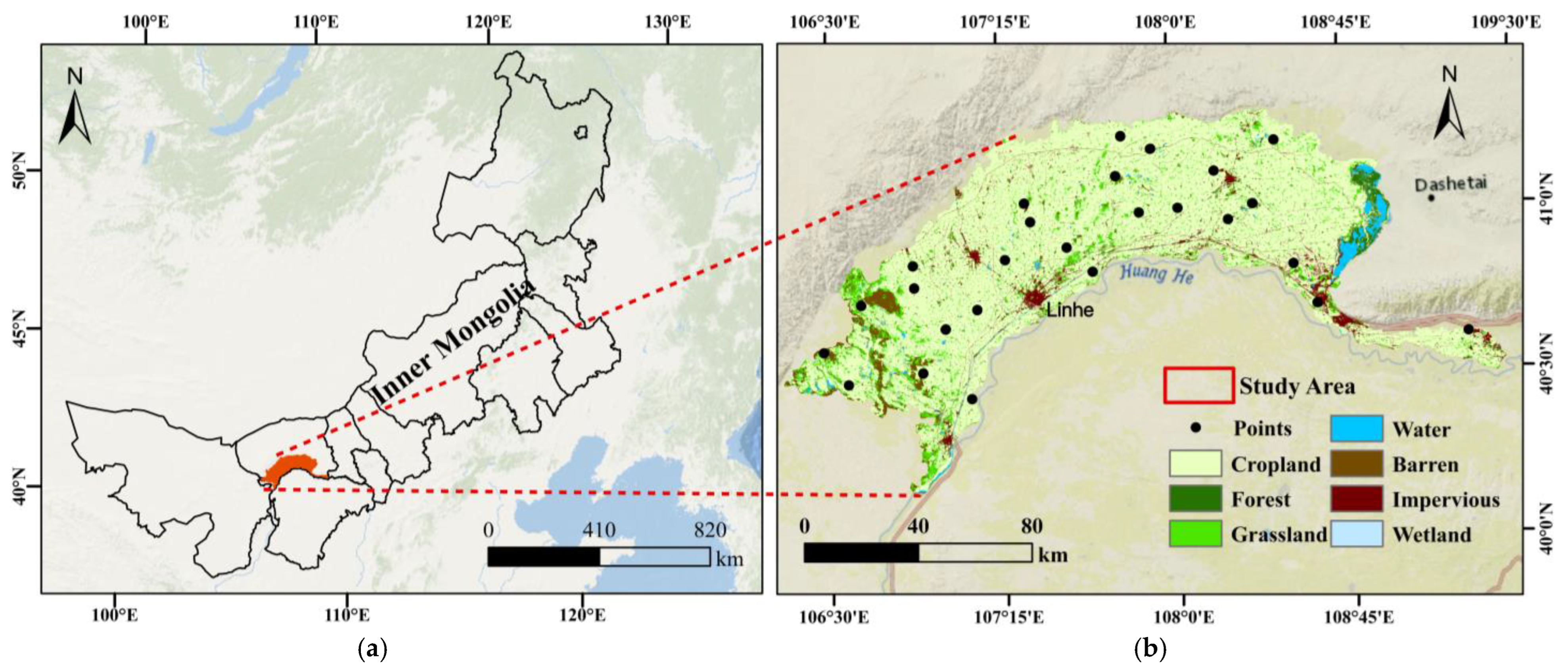
2.1. Research Area Overview

As shown in Figure 1, the study area is the Hetao Plain in Inner Mongolia, China, located between longitudes 106°7′44″ E and 106°52′20″ E, and latitudes 38°37′56″ N and 39°5′23″ N. It is one of the most important grain-producing regions in northern China and the largest irrigated area in the country, with water sourced mainly from the Yellow River. Elevation ranges from 1100 to 1500 m, and the terrain is gentle. Groundwater collects in low areas and raises the water table. In addition, because the area is arid to semi-arid with strong sunlight and high evaporation, soil salts move upward with the evaporating water, build up at the surface, and cause serious salinization. Therefore, the region is a typical area for the distribution of saline–alkali soils [39]. The location and coordinates of the study area were obtained using Google Earth Pro (version 7.3.6, Google LLC., Mountain View, CA, USA).

2.2. Data Collection and Processing

2.2.1. On-Site Hyperspectral Data and Soil Sample Collection

The experiment was conducted in November 2023 in the Hetao region. The ground-truth soil samples were collected during the brightest hours of the day (10:00–15:00 local time) under windless, cloudless skies. After sampling, hyperspectral imaging was used to acquire spectral data from the samples. In this study, the Pika L hyperspectral imaging system (Resonon Inc., Bozeman, MT, USA) was used to collect soil spectral data [40]. The system has 138 spectral channels, with a wavelength range of 450–998 nm and a spectral resolution of 4.8 nm. The exposure time was set to 10 ms, with 6 pixel mixing iterations. The vertical distance from the scanning probe to the sample was 60 cm. Prior to measurement, the spectral images were calibrated by capturing target and all-black images for correction to eliminate noise caused by the light source and dark current. During data collection, the sampling points and hyperspectral reflectance were systematically numbered and recorded, and photos of vegetation and soil salinization at each sampling point were taken as experimental references. A total of 29 surface soil samples were collected and sealed in self-sealing bags.

2.2.2. Landsat 8 Multispectral Data Preprocessing

The Landsat 8 data for the study area were atmospherically corrected and clipped to the study boundary. Four bands—blue (450 nm), green (550 nm), red (670 nm), and near-infrared (850 nm), conforming within 450–998 nm—were extracted to generate a 4-band MSI image in GeoTIFF format. Landsat 8 preprocessing (atmospheric correction and image clipping) was performed using ENVI software (version 5.6, Harris Geospatial Solutions, Boulder, CO, USA).

2.2.3. Data Collection of Soil Water-Soluble Ions

The collected soil samples were naturally air-dried in a ventilated, cool, and dry environment. Afterward, the samples were crushed using a rubber mallet and passed through a 200-mesh sieve to remove debris, gravel, and other impurities. A 25 g portion of the sieved sample was weighed, and 125 mL of distilled water (with a soil-to-water ratio of 1:5) was added. The mixture was shaken and allowed to stand for 8 h, after which it was filtered to obtain the supernatant. Chemical titration experiments were conducted on the supernatant to determine ion concentrations. The concentrations of Ca²⁺ and Mg²⁺ were determined using the EDTA titration method, with EDTA (analytical grade, Aladdin Reagent Co., Ltd., Shanghai, China), CO₃²⁻ was measured using a double indicator neutralization titration with phenolphthalein and methyl orange (Sinopharm Chemical Reagent Co., Ltd., Shanghai, China), and SO₄²⁻ was measured by EDTA indirect complexometric titration. Standard and control samples were used for each batch of ion content analysis to ensure the accuracy of the results. All titrations followed the Chinese standards LY/T 1251-1999 and GB/T 7477-1987, which are widely adopted for routine soil-ion determination. Although we did not perform additional spike-recovery tests because of limited extract volume, duplicate titrations of randomly selected samples showed highly consistent results (RSD < 4%), consistent with the precision reported for these standards. Following the practice in similar studies, we propagate a conservative laboratory uncertainty of ±5% of each measured concentration into the subsequent modelling stage. Since CO₃²⁻ easily forms precipitates with Ca²⁺ and Mg²⁺ in slightly alkaline conditions, the concentration of CO₃²⁻ was not detected in some of the soil samples.

Table 1. Descriptive statistical analysis results of four water-soluble ions in soil.

Ions	Mean (g/kg)	Median (g/kg)	SD (g/kg)	MAD (g/kg)	Best-Fit Distribution (Shape, Scale)	Skewness	Shapiro–Wilk p
Ca2+	1.53	1.52	0.72	0.61	Weibull (1.36, 1.60)	−0.07	0.91
CO32−	1.07	1.09	0.51	0.42	Weibull (1.38, 1.12)	0.03	0.76
Mg2+	0.61	0.72	0.31	0.27	Weibull (1.78, 0.67)	−0.23	0.45
SO42−	2.03	2.39	1.01	0.75	Weibull (1.18, 2.06)	−0.23	0.45

summarizes the statistical characteristics of ion concentrations. All ions show near-symmetric distributions (skewness between −0.23 and 0.03), with consistent mean–median values. Normality tests (p > 0.45) suggest approximate normality, though Weibull fits offer slightly better AIC. The SD-to-MAD ratios fall between 1.15 and 1.20, close to the expected value for normal data (~1.253), suggesting light tails and the absence of extreme values, ensuring statistical robustness in the presence of mild asymmetry or measurement variability.

2.3. Hyperspectral Data Reconstruction Method

Common interpolation methods (spline interpolation, linear interpolation, and nearest neighbor interpolation) tend to generate intermediate values based on known data points. These methods are simple to implement but have limited accuracy and cannot capture the nonlinear information and complex fine-grained features in hyperspectral data [41]. In recent years, Generative Adversarial Networks (GANs) and Transformer models have shown the ability to model nonlinear relationships between inputs and outputs [42,43,44,45], making it possible to reconstruct high-resolution hyperspectral data from low-resolution Landsat 8 multispectral data. However, these methods require high stability and quality of the generated data [46,47,48].

Therefore, this paper proposes a model that combines the wavelet transform and Transformer (wavelet-Transformer). By utilizing the Transformer’s self-attention mechanism to capture the complex dependencies between wavelets better, the model aims to improve accuracy and enhance the robustness of the model in spectral data processing [49]. The method first performs multiscale feature extraction and denoising preprocessing of multispectral data using wavelet transform, and then feeds the processed features into the Transformer model to capture the deep dependencies between different bands, thus realizing high-precision reconstruction of Landsat 8 multispectral data to hyperspectral data in the range of 450–998 nm.

The wavelet transform enables multi-resolution analysis of signals, providing localized information in both the time and frequency domains [50]. It performs well in data denoising, improving input quality by cutting redundancy while keeping signal edges [51]. This makes the inputs for later Transformer models more concise and informative [52]. In this study, Daubechies is chosen as the mother wavelet to balance edge preservation and frequency-localized feature extraction, making it suitable for this type of remote-sensing image data. The mother wavelet is first decomposed into three levels to denoise and extract multiscale spectral features. The wavelet-processed features are then fed into the Transformer model, which uses self-attention to capture dependencies between spectral bands and generate high-resolution outputs [53]. This preprocessing step plays a crucial role in improving model performance. By removing high-frequency noise and enhancing spectral edges, the wavelet-transformed features provide a cleaner and more structured input for the Transformer to learn from. This enhances the model’s ability to capture inter-band dependencies and avoids overfitting on noisy signals.

The Transformer component uses four encoder layers, eight attention heads, a model dimension of 64, and a dropout rate of 0.1. These hyperparameters were selected based on commonly used configurations in spectral deep learning literature and adjusted empirically through preliminary testing to match the scale of our data [54,55,56]. This configuration provides a balance between model expressiveness and computational efficiency. The loss function was MSE, optimized using Adam (initial learning rate = 1 × 10⁻⁴), with batch size 16. Training was performed for up to 100 epochs with early stopping (patience = 10). The full architecture of the wavelet-Transformer is shown in Figure 2. In the inset illustrating the Wavelet-Transformer kernel, the asterisk on ψ*(t) indicates the complex conjugate of the mother wavelet ψ(t). For comparison, we evaluated this model alongside spline, linear, and nearest-neighbor interpolation methods as well as a standard Transformer model, using R² and MSE as evaluation metrics. The model is implemented in Python (v3.10.6).

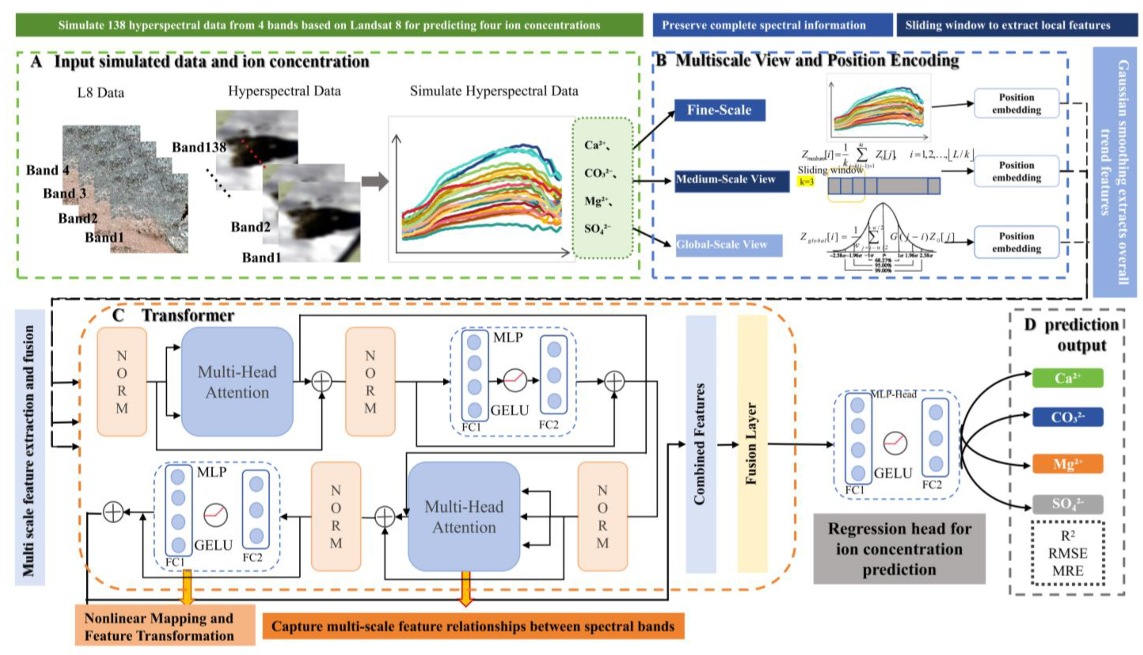
2.4. Soil Water-Soluble Ion Inversion Model MSATransformer

Soil water-soluble ions exhibit spectral properties characterized by significant inter-band correlations [57]. Although the spectral resolution is improved in the hyperspectral data reconstructed from Landsat 8, the number of bands also increases dramatically. This expansion leads to substantial spectral redundancy, especially in regions with minimal spectral variation. The correlations between different bands may have complex changes at multiple scales, requiring models that can both capture local changes between fine-grained bands and extract global trends [30]. The key is how to effectively utilize the full information of hyperspectral data while avoiding the effects of band redundancy and noise on model inversion performance [58].

Therefore, to address the characteristics of hyperspectral data analysis, this paper improves on the Transformer and proposes an MSATransformer model based on a multi-scale fusion mechanism between spectral bands. The model extracts local features, regional correlations, and overall trends of hyperspectral data through three views: fine-grained, mesoscale, and global scales. This multi-scale representation enables more efficient capture of the complex characteristics of hyperspectral data and thus enhances the inversion accuracy of soil water-soluble ion concentration. In addition, the multiscale nature of the reconstructed hyperspectral data may lead to information imbalance between different views. MSATransformer dynamically weights the features of different scales through the cross-scale fusion mechanism and assigns weights according to the contributions of different bands and views to avoid over-concentration of information in a particular view or band [59,60]. The fusion retains the information of local band changes and strengthens the global spectral trend, thus significantly improving the adaptability to multispectral reconstruction of hyperspectral data. The overall structure of the model consists of the following modules: input embedding and position encoding, multi-scale view generation, multi-scale attention mechanism, fusion, and inversion. The structure of the MSATransformer model is shown in Figure 3 below.

The specific implementation process of the model is as follows:

Step 1: Input Feature Embedding.

The input data consists of a sequence of hyperspectral bands $X\in {ℝ}^{N\times L}$. After passing through the embedding layer and position encoding, it is transformed into an embedded sequence $Z_0\in {ℝ}^{L\times d}$ Equation (1):

$$Z_0=W_{e}X+b_e+P$$

(1)

where N is the number of samples and L is the number of spectral bands, which are 29 and 138, respectively, in this study.

For each sample $X_i=\{x_{i,1},x_{i,2},\dots ,x_{i,L}\}$, its input is mapped to a feature sequence $E_i=W_e{X}_i+b_e,\hspace{1em}{E}_i\in {ℝ}^{L\times d}$ after passing through the embedding layer. Here, $W_e\in {ℝ}^{d\times 1}$ represents the learnable weight matrix, $b_e\in {ℝ}_d$ is the bias vector, and d denotes the embedding feature dimension, which is used to map the spectral bands to a high-dimensional feature space.

To preserve the sequential relationship of the spectral bands, a sine position encoding $P\in {ℝ}^{L\times d}$ is added, defined as shown in Equation (2):

$$P\left(pos,2i\right)=\sin ({\displaystyle \frac{pos}{10,{000}^{2i/d}}}),P\left(pos,2i+1\right)=\cos ({\displaystyle \frac{pos}{10,{000}^{2i/d}}})$$

(2)

The final input features are expressed as shown in Equation (3):

$$Z_0=E+P,\begin{array}{cc}& Z_0\in {ℝ}^{L\times d}\end{array}$$

(3)

Step 2: Multi-Scale View Generation.

To better capture the multi-level correlations between spectral bands [61], three multi-scale views are generated as follows:

• Fine-Scale View: This view retains the original embedded sequence $Z_0$, i.e., $Z_{fine}=Z_0$
• Medium-Scale View: This view is generated by performing sliding window down-sampling on $Z_0$, where the window size is k. It is defined as shown in Equation (4):

  $$Z_{medium}[i]={\displaystyle \frac{1}{k}}{\displaystyle \sum _{j=k(i-1)+1}^{ki}{Z}_0[j]},\hspace{1em}\hspace{1em}i=1,2,\dots ,⌊L/k⌋$$

  (4)

  where k is the window size (in this study, k = 3), and the downsampled dimension after this operation is $⌊L/k⌋\times d$.
• Global-Scale View: The global view is obtained by applying Gaussian smoothing to $Z_0$ to capture the global features. It is defined as shown in Equation (5):

  $$Z_{global}[i]={\displaystyle \frac{1}{w}}{\displaystyle \sum _{j=i-w/2}^{i+w/2}G(j-i)Z_0[j]}$$

  (5)

  where $G(j-i)$ represents the Gaussian kernel weights, and $\omega$ is the window size (in this study, $\omega$ = 7).

Step 3: Multi-Scale Attention Mechanism.

Each of the three multi-scale views is independently fed into the Transformer encoder for individual processing.

Query (Q), Key (K), and Value (V) Generation: for each view $Z\in {ℝ}^{L\times d}$, generate the query, key, and value through linear projections as follows: $Q=Z{W}_Q,K=Z{W}_K,V=Z{W}_V$, where $W_Q,W_K,W_V\in {ℝ}^{d\times d_k}$ is a learnable weight matrix.

Attention Weight Calculation: the attention weights are computed using the dot-product attention mechanism, as shown in Equation (6):

$$Attention(Q,K,V)=softmax({\displaystyle \frac{Q{K}^T}{\sqrt{d_k}}})V$$

(6)

where $d_k$ is the dimension of the key vector.

Multi-Head Self-Attention Mechanism: the results from multiple attention heads are concatenated and projected as shown in Equation (7):

$$MHA(Z)=Concat(hea{d}_1,\dots ,hea{d}_h)W_O$$

(7)

where $W_O\in {ℝ}^{h{d}_k\times d}$ is the output projection matrix, and h is the number of attention heads. Each head is computed as the attention mechanism described earlier.

Feed-Forward Network: a two-layer fully connected network is applied independently at each position as shown in Equation (8):

$$FFN(x)=ReLU(x{W}_1+b_1)W_2+b_2$$

(8)

The output of the encoder is defined as shown in Equation (9):

$$H_{fine},H_{medium},H_{global}=Transformer(Z_{fine}),Transformer(Z_{medium}),Transformer(Z_{global})$$

(9)

Step 4: Cross-Scale Fusion.

The features from the three scales are dynamically weighted using another self-attention mechanism, as shown in Equation (10):

$$H_{fused}=Attention(H_{fine},H_{medium},H_{global})$$

(10)

where $H_{fine},H_{medium},H_{global}$ represent the fine-scale, medium-scale, and global-scale features, respectively. This step allows the model to learn how to combine the different scales of information in an optimal way.

Step 5: Regression Prediction.

The fused features $H_{fused}$ are then passed through a fully connected layer to complete the regression task, as shown in Equation (11):

$${\widehat{y}}_i=MLP(H_{fused})$$

(11)

where ${\widehat{y}}_i$ is the predicted output. The final ion concentration predictions are generated using a two-layer multilayer perceptron (MLP) with ReLU activation, which maps the fused multi-scale features to the output space.

The implementation details of the MSATransformer model are as follows: embedding dimension d = 64 for mapping spectral data into a high-dimensional feature space; number of heads h = 8; and number of encoder layers N = 3, used to capture multi-layer spectral features. In addition, in order to construct meso-scale and global-scale features, the sliding window size is set to k = 3 and the Gaussian smoothing kernel size is set to w = 7. The loss function is the mean-square error (MSE), and the optimizer uses Adam (with an initial learning rate of lr = 1 × 10⁻⁴), a batch size of 16, and a maximum number of 100 training epochs. Early-stopping tolerance (patience) is set to 10. The MSATransformer was implemented using the PyTorch deep learning framework (v1.13.1; https://pytorch.org/), with training and evaluation code developed in Python (v3.10.6).

2.5. Model Evaluation

The model was evaluated using the Coefficient of Determination (R²), Mean Square Error (MSE), Root Mean Square Error (RMSE), and Mean Relative Error (MRE). These metrics are widely used in remote sensing regression tasks to assess model accuracy and stability. In general, a higher R² and lower MSE, RMSE, and MRE indicate better predictive performance. The entire dataset was randomly divided into a training set (80%) and an independent test set (20%) using a fixed random seed of 42. All reported performance metrics are point estimates calculated on this fixed test set.

3. Results

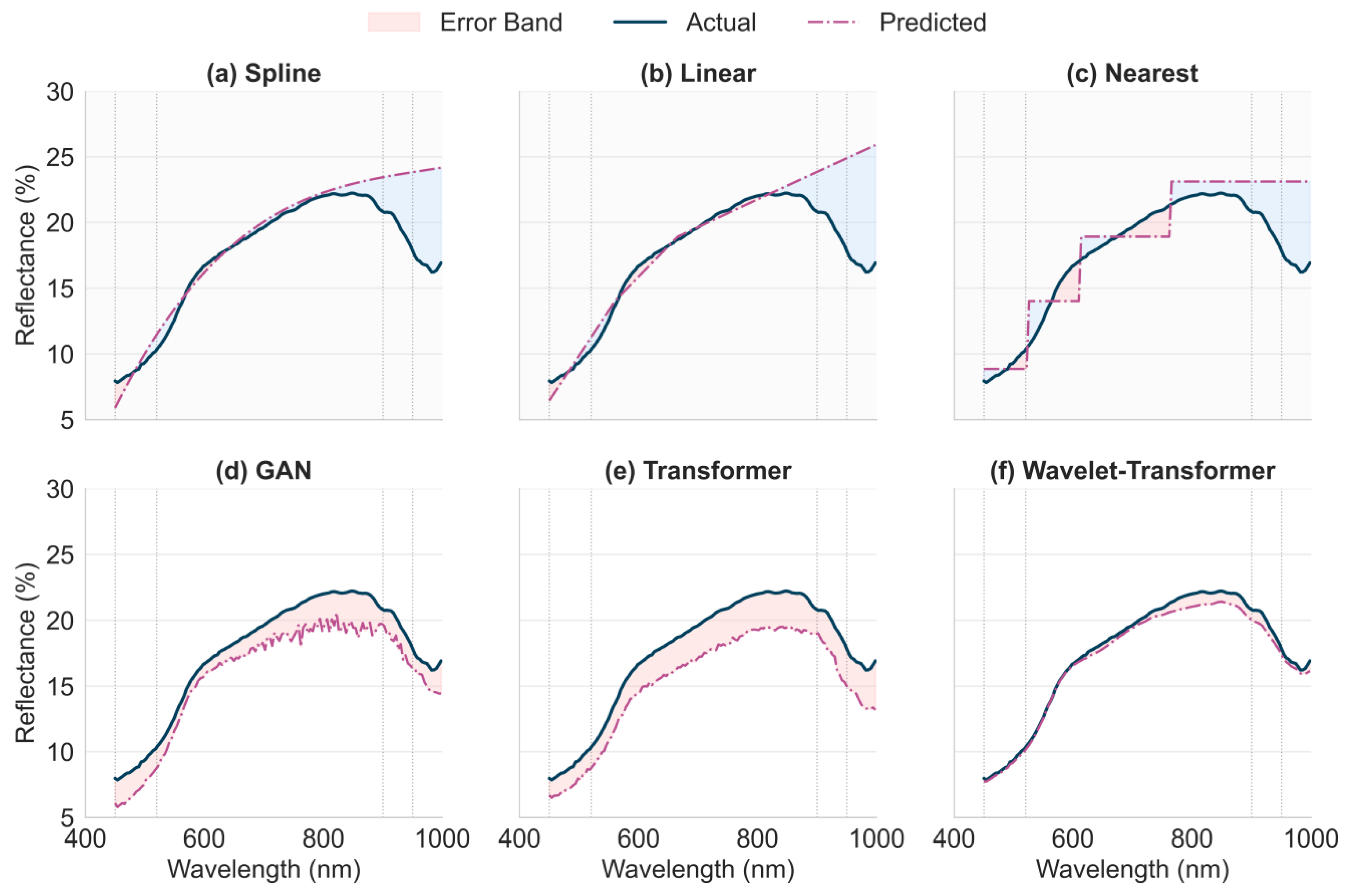
3.1. Comparison of Reconstructed Ground-Based Hyperspectral Data with Measured Hyperspectral Data

Table 2. Evaluation of different reconstruction methods.

Method	R2	MSE
Spline Interpolation	0.67	6.38
Linear Interpolation	0.65	6.67
Nearest Neighbor Interpolation	0.52	9.30
GAN	0.83	3.29
Transformer	0.71	5.68
Wavelet-Transformer	0.98	0.31

compares the R² and MSE metrics of three traditional interpolation methods and three deep learning models in hyperspectral reconstruction. From the fitting results, it can be seen that the R² of the traditional interpolation method can only reach 0.52–0.67, and the MSE is 6.38–9.30, which makes it difficult to reconstruct complex nonlinear spectral features, and the deep learning model performs significantly better than the interpolation method, in which the reconstruction accuracy of Transformer model for hyperspectral data reaches R² = 0.71, MSE = 5.68. The reconstruction accuracy of the GAN reaches R² = 0.83, MSE = 3.29. Our wavelet-Transformer model has R² as high as 0.98 and MSE as low as 0.31. It is significantly ahead of other models, and the accuracy of hyperspectral reconstruction is greatly improved.

Figure 4 illustrates the residual distribution and normal distribution curves of different spectral reconstruction methods. Several interpolation methods show skewed residual distributions with a wide range, indicating their inability to capture the spectral fine-grained features of the soil. Therefore, they are not effective in hyperspectral data reconstruction tasks. In contrast, the GAN and Transformer models exhibit long-tailed distribution, although they perform better in capturing global trends. The wavelet-Transformer model has the most concentrated distribution of residuals, the median tends to be close to the value of 0, the IQR is the narrowest, and the normal distribution curve is almost the same as the box plot, which is characterized by a standard normal distribution. These results further show that the wavelet-Transformer model has strong capabilities in noise suppression and feature extraction, achieving the best performance in hyperspectral data reconstruction.

Figure 5 visualizes the difference between the reconstructed hyperspectral data and the measured ground-based hyperspectral data of the agricultural saline field. The interpolation method has an obvious step effect with amplitude deviation. In contrast, the GAN model performs better in the wavelength range of 450–600 nm, but does not fit the measured data well enough in the interval of 600–900 nm. This is likely because the model fails to learn detailed spectral features and cannot effectively capture the complex relationship between wavelengths and the reflectance, leading to notable deviation from the actual values. In addition, the measured and reconstructed spectral curves of the Transformer model are more consistent with each other in the general trend. However, the deviation of the numerical fit at the wave out is still large. In contrast, the wavelet-Transformer model proposed in this paper achieves high reconstruction accuracy across the entire spectral range. It accurately reproduces short-wavelength peaks, mid-wavelength smoothing, and long-wavelength decreasing trends in the measured hyperspectral curves. It not only retains the smoothness of local fluctuations but also utilizes the multi-resolution analysis advantage of the wavelet transform, which effectively enhances the feature extraction ability of the model in different band intervals.

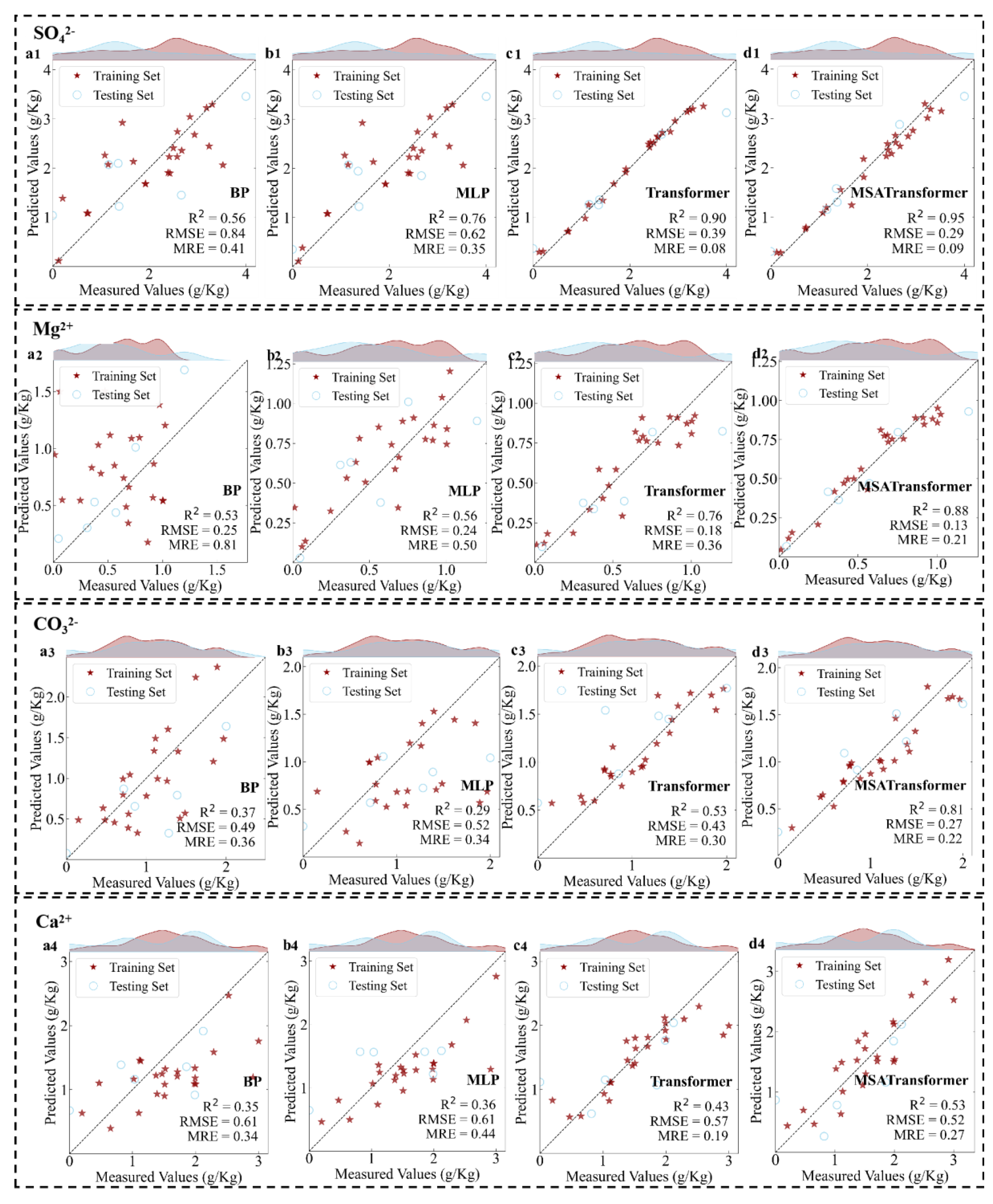
3.2. Inversion Accuracy Analysis of Water-Soluble Ions in Agricultural Soils

The four main soil water-soluble ions (Ca²⁺, CO₃²⁻, Mg²⁺, SO₄²⁻) were analyzed under the MSATransformer architecture based on Landsat 8 multi-spectral data and reconstructed hyperspectral data for inversion analysis, respectively. In Figure 6, subplot a represents the magnitude of the R² boost from Landsat 8 multispectral data (represented as MSI in the Figure 6) to reconstructed hyperspectral data (represented as HSI in the Figure 6). The coefficients of determination of all four ions are enhanced when reconstructed hyperspectral data are the inputs, with the enhancement of R² being particularly pronounced for Mg²⁺ and SO₄²⁻, which are improved by 0.22 vs. 0.21, respectively. Subfigure (b) shows the prediction results of different ions in the form of a heat map for both the MSI and the reconstructed HSI conditions. The R² (reconstructed HSI) columns are all higher than the R² (MSI) columns; similarly, the RMSE (HSI) columns are all lower than the RMSE (MSI) columns. Subfigure (c) denotes the relative error reduction in the two inputs, where SO₄²⁻ has an RMSE of 0.64 at MSI and only 0.29 at HSI, which is a reduction of 55%. The error reduction in Ca²⁺, CO₃²⁻ and Mg²⁺ can reach 32%, 29%, and 55%, respectively. Subfigure (d) denotes the superposition of residual kernel density profiles for the same ion under different input conditions. Under the conditions of reconstructed hyperspectral data, the residual kernel density profiles for each ion are more concentrated, with higher peaks and narrower tails in the residual distributions, indicating that the HSI captures less noise in the response band.

In addition to traditional performance metrics, we also assessed the statistical significance of the correlation between predicted and measured values using Pearson’s r and p-value. Among the four ions, CO₃²⁻, Mg²⁺, and SO₄²⁻ showed statistically significant correlations (p < 0.01), while Ca²⁺ had a lower but still positive correlation (r = 0.93, p = 0.02), likely due to its weaker spectral signature. The results are summarized in

Table 3. Pearson correlation coefficients and p-values between predicted and measured ion concentrations based on reconstructed hyperspectral data (HSI).

Ion	Pearson r	p-Value
Ca2+	0.93	0.02
CO32−	0.94	<0.01
Mg2+	0.96	<0.01
SO42−	0.98	<0.01

, supporting the overall robustness of the predictions based on reconstructed hyperspectral data (HSI).

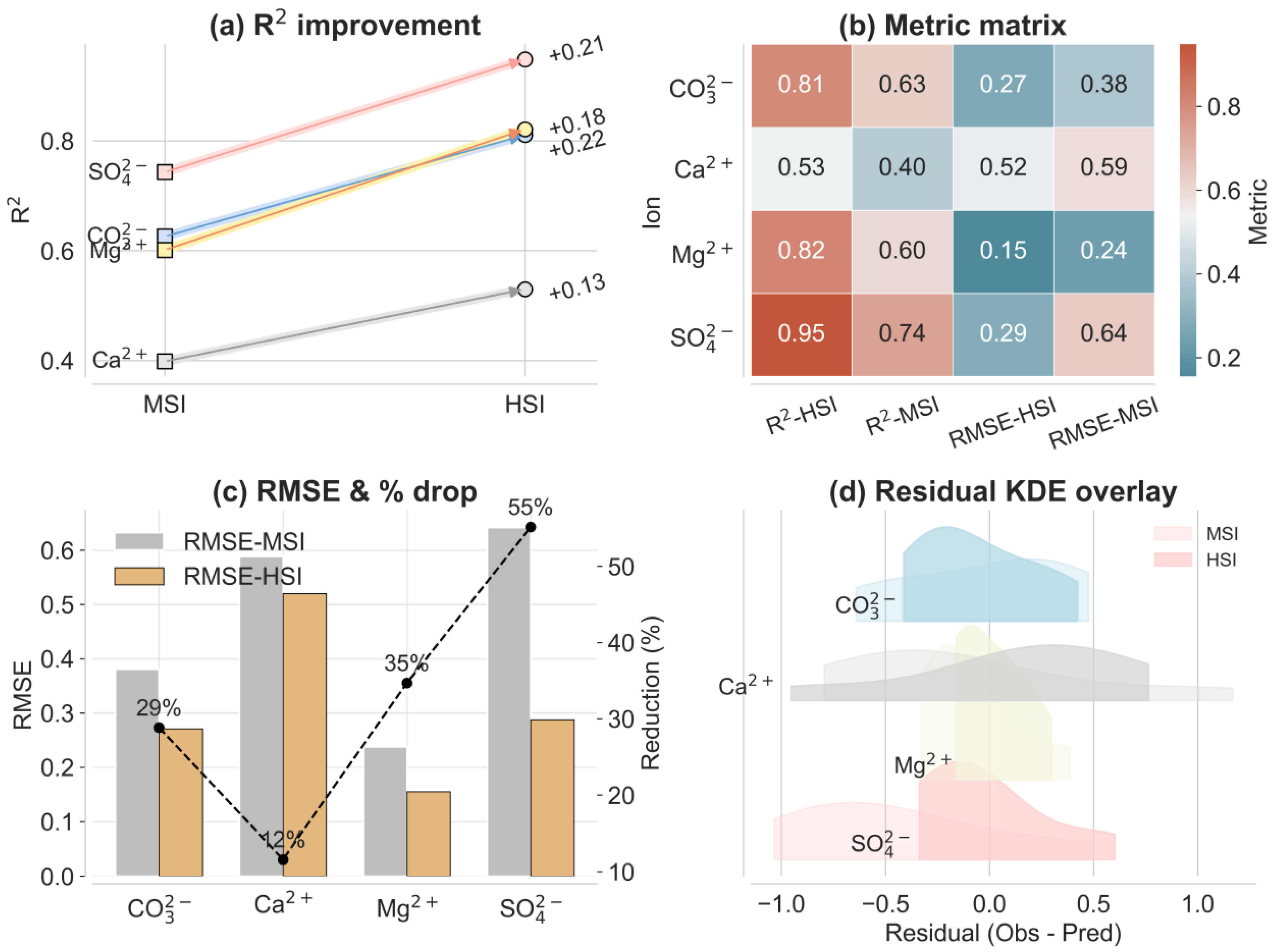
3.3. Residual Structure Analysis of Water-Soluble Ion Inversion Based on MSI and HSI

As shown in

Table 4. Residual statistics of the ion test set based on MSI and reconstructed HSI.

Ion	MSI				HSI
	Bias	σ	Skewness	Kurtosis	Bias	σ	Skewness	Kurtosis
Ca2+	0.11	0.63	–1.12	2.99	−0.13	0.55	0.96	2.90
CO32−	0.01	0.42	0.32	1.60	0.06	0.29	−0.52	1.86
Mg2+	0.09	0.24	−1.19	3.11	−0.01	0.17	−0.51	1.84
SO42−	0.44	0.51	−0.82	2.46	0.02	0.31	−1.03	2.82

, the mean of the predicted residuals of the test set of reconstructed hyperspectral data for the water-soluble ion content of agricultural soils is closer to 0 under the MSATransformer model, and the standard deviation is significantly reduced. For example, for the SO₄²⁻ ion, the Bias is +0.440 under MSI, and the band is intense, with σ reaching 0.511; however, the Bias decreases to +0.021 under the reconstructed HSI, and σ shrinks to 0.314. Bias close to 0 and a significant narrowing of σ were achieved for Mg²⁺ and Ca²⁺ as well, while σ for CO₃²⁻ decreased from 0.416 to 0.289. It is shown that the reconstructed hyperspectral data effectively suppresses the random errors, and in general, the dispersion of the residual distribution of the reconstructed hyperspectral data is significantly weakened, which effectively improves the inversion accuracy and stability of the model.

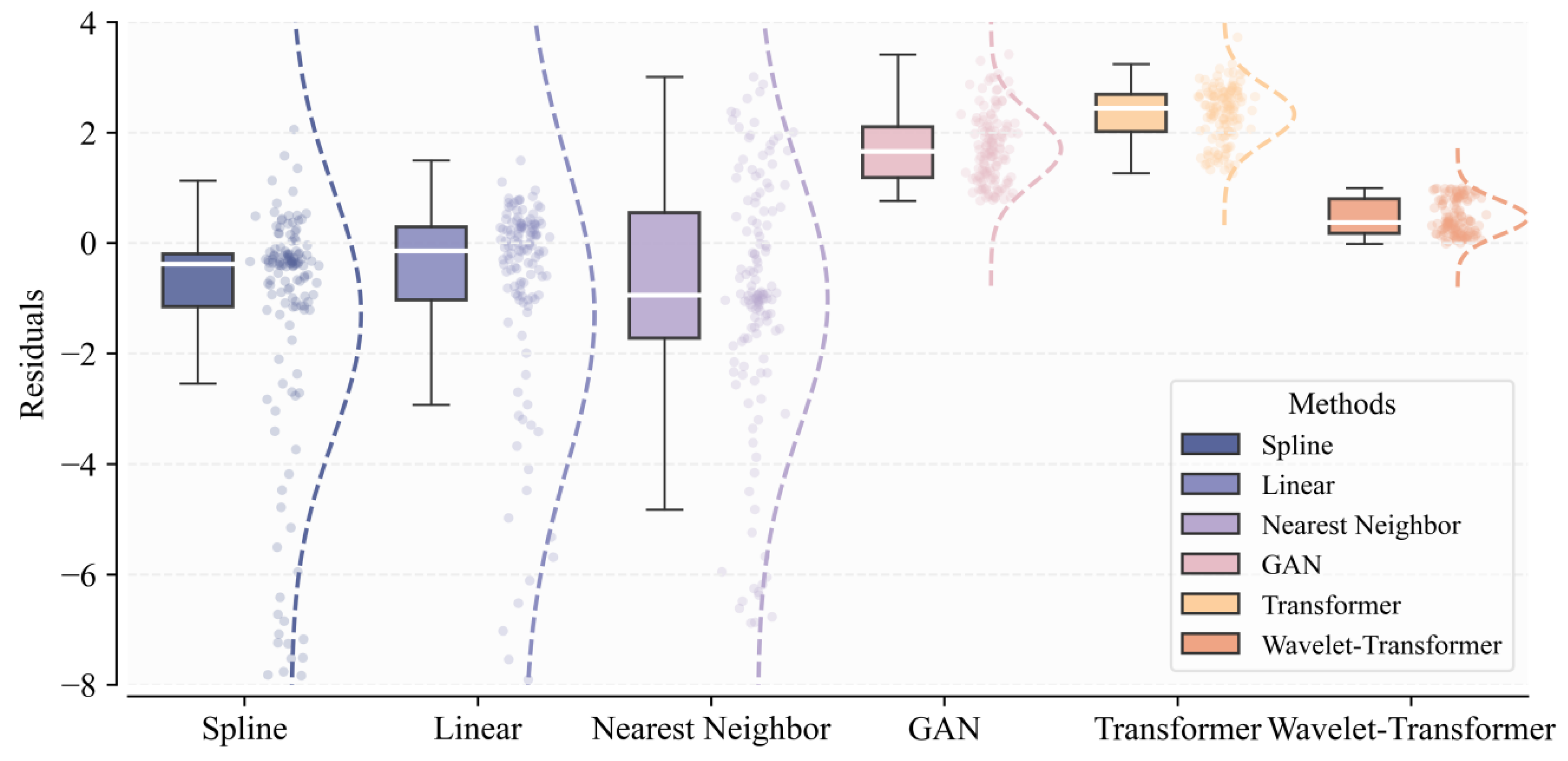
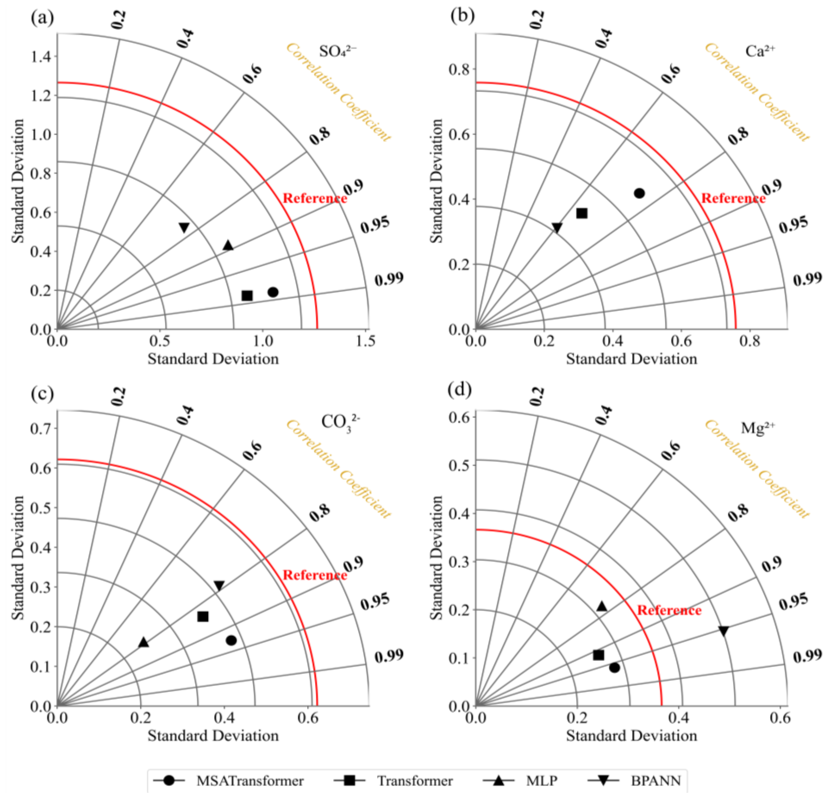
3.4. Comparative Analysis of Models

To further validate the superiority of the MSATransformer model in soil water-soluble ion inversion tasks, this study systematically compared it with the BP neural network, the MLP neural network, and the Transformer model. The comparison results are shown in Figure 7. The MSATransformer model achieved the highest R² values and the lowest RMSE and MRE values in all the inversion tasks for all the ions through three-view multi-scale extraction and cross-scale fusion. MSATransformer shows significant improvement in the inversion accuracy of both training and test sets by introducing multi-scale feature extraction and cross-scale fusion mechanisms. In the inversion of weakly spectroscopically characterized ions (Ca²⁺ and CO₃²⁻), MSATransformer shows a clear advantage with the test set R² of 0.53 and 0.81, which is much higher than those of BP (R² = 0.35 and 0.37), MLP (R² = 0.36 and 0.29), and the original Transformer (R² = 0.43 and 0.53). Meanwhile, the inversion errors were significantly reduced, e.g., RMSE and MRE were 0.52 and 0.27 for Ca²⁺ and 0.27 and 0.22 for CO₃²⁻, respectively. For ions with significant spectral properties (Mg²⁺ and SO₄²⁻), the MSATransformer also showed excellent performance. The test set achieved R² of 0.88 and 0.95, RMSE of 0.13 and 0.29, and MRE of 0.21 and 0.09, respectively. These results are significantly better than the BP and MLP models (R² of 0.53 and 0.56 for Mg²⁺ and 0.56 and 0.76 for SO₄²⁻), and also better than the original Transformer model (R² of Mg²⁺ = 0.76 and R² = 0.90 for SO₄²⁻). In summary, the MSATransformer significantly improves the accuracy, stability, and generalization ability of soil water-soluble ion inversion with the assistance of reconstructed hyperspectral data by virtue of the multi-scale feature extraction and cross-scale fusion mechanism, proving the effectiveness of this paper’s method In accurately monitoring salinized soils.

To further demonstrate the practical prediction capability of the MSATransformer model,

Table 5. Predicted and measured values of four ions on the test set using the MSATransformer model.

SO42−		CO32−		Ca2+		Mg2+
Actual	Predicted	Actual	Predicted	Actual	Predicted	Actual	Predicted
2.66	2.88	0.86	0.91	1.98	1.84	0.75	0.79
0	0.31	2.01	1.81	0.81	0.26	0.05	0.06
1.36	1.58	1.28	1.51	1.85	1.16	0.31	0.42
4	3.45	0.11	0.25	2.12	2.12	1.2	0.92
1.37	1.31	1.38	1.21	1.03	0.78	0.57	0.47
1.16	1.15	0.72	1.09	0	0.86	0.37	0.36

lists the predicted and actual ion concentrations on the test set. The results show that the predicted values are generally close to the measured values. Among them, the prediction errors for SO₄²⁻ and Mg²⁺ remain small across both high and low concentration ranges, indicating good accuracy and robustness.

Figure 8 illustrates the Taylor diagrams of the four models on different soil water-soluble ions, with radial distance indicating the standard deviation, grade angle indicating the correlation coefficient, and the red curve indicating the reference value. As can be seen from the Taylor diagrams, the MSATransformer model is closest to the reference value. Except for the fluctuations of CO₃²⁻ ions, which are underestimated overall, for the three ions (Ca²⁺, Mg²⁺, and SO₄²⁻), the MSATransformer model maintains a low error while having a high correlation, and the overall performance is better than MLP and BPANN models.

4. Discussion

4.1. Comparison of Reconstructed Hyperspectral Data with Real Data

Landsat 8 data, with its low spectral resolution, fails to capture complex spectral features, leading to significant accuracy issues in tasks such as soil water-soluble ion concentration prediction. In contrast, hyperspectral data provides extremely high spectral resolution, allowing for detailed characterization of ion spectral characteristics across different bands. However, the high cost of obtaining hyperspectral data, limited coverage, and complex data processing make its large-scale application significantly restricted [61]. Therefore, in order to enhance prediction accuracy within limited costs, research workers have attempted to use deep learning models to improve prediction accuracy based on multispectral data. A typical approach is spectral reconstruction or data fusion, which jointly models multispectral and hyperspectral data to reconstruct or enhance hyperspectral features [15,16]. This approach can reduce data acquisition costs while improving prediction accuracy. However, different deep learning methods exhibit significant variations in their performance in reconstructing data generation. Convolutional Neural Networks (CNNs) are effective at extracting spatial features when processing spectral image data. However, in one-dimensional data processing, they fail to fully utilize the continuity and sequential features of the data, which is particularly evident when reconstructing hyperspectral data from low spectral resolution multispectral data. As a result, CNNs cannot comprehensively capture the continuous spectral changes in spectral reconstruction tasks [30]. The Generative Adversarial Network (GAN) model excels in data generation tasks, but it is highly sensitive to model architecture and hyperparameters. Additionally, GANs are prone to mode collapse, resulting in limited diversity in the reconstructed data and reduced generalization capability [42]. BP neural networks are less efficient to train when dealing with large-scale data. Although newer architectures such as GANs have shown promising results in some experimental studies, they still struggle to efficiently capture complex spectral patterns in remote sensing tasks [35,62,63]. In this paper, hyperspectral data are reconstructed using a wavelet-Transformer model. Compared to traditional approaches such as interpolation and the live response function method—which rely on endmember-based modeling and make simplifying assumptions—our method provides greater flexibility, captures complex nonlinear spectral features more effectively, and generates results that closely align with field-measured spectra.

4.2. Model Comparison

Several studies have used machine learning and deep learning approaches to invert the concentrations of soil salts and water-soluble ions. However, these models do not explain the heterogeneity well. Heterogeneity refers to the variability or difference present in the data. It also means that the model may not be able to effectively invert the variation or local differences in the concentration of water-soluble ions [19,64,65,66,67]. BP models perform poorly in weak spectral characterization ion inversion due to their reliance on only shallow network structures, which makes it difficult to fully capture the complex nonlinear relationships in spectral data [62,68]. MLP lacks spectral sequence feature extraction, although it has some nonlinear modeling capability [36]. Whereas the original transformer has some advantages in capturing long-range dependencies, it fails to fully utilize the information from hyperspectral data, resulting in limited inversion accuracy for global trend modeling [47,50,69]. Compared with other models, the MSATransformer proposed in this study shows advantages in soil water-soluble ion inversion, not only because wavelet decomposition enhances spectral sparsity and isolates local signal components related to specific ion absorption features, but also in two main aspects. First, through multi-scale view generation, MSATransformer can capture spectral features of soil at different scales and focus on some weak spectral variations related to ion concentrations. This helps the model recognize informative spectral data and improves inversion accuracy. Second, MSATransformer can dynamically adjust attention weights for different bands and features, reduce the interference of redundant information, and improve adaptability to hyperspectral data. This provides higher accuracy and robustness in modeling complex spectral dependencies. Therefore, compared with models that lack this kind of targeted feature selection, MSATransformer achieves better generalization and accuracy in ion concentration inversion. In addition to predictive accuracy, computational efficiency is also an important consideration for practical deployment. The MSATransformer model is computationally lightweight, with fast inference (<10 s per sample) and moderate training time (4–5 min per ion) on a single NVIDIA RTX 2080Ti GPU. We also verified that the model can be trained on standard CPUs, which, although slower, supports its potential for broader deployment in real-world applications.

4.3. Soil Water-Soluble Ion Inversion

The inversion of soil water-soluble ions refers to the process of estimating the concentration of water-soluble ions in soil using remote sensing techniques or modeling approaches. This study focuses on saline soils in the Hetao region as the primary research subject. The saline–alkali soils of the Hetao Plain are predominantly composed of sodium salts, carbonates, and other components, with a pH typically exceeding 8.0, indicating strong alkalinity [39]. These soil characteristics dictate the concentration, distribution, and interactions of water-soluble ions with other soil constituents. In saline–alkali soils, ions such as Mg²⁺ and SO₄²⁻ often exhibit pronounced spectral absorption features, particularly showing distinct absorption peaks in the visible to near-infrared wavelength range [57,70,71]. In contrast, Ca²⁺ and CO₃²⁻ demonstrate weaker spectral responses, with their signals dispersed across multiple bands. Additionally, the concentration variations of Ca²⁺ exhibit a certain degree of coupling with Mg²⁺ and CO₃²⁻, complicating the prediction process. This coupling effect may lead the model to rely on indirect spectral cues from these related ions rather than the spectral characteristics of Ca²⁺ itself, thereby significantly impacting the accuracy of spectral models.

The Hetao irrigation district can represent typical irrigated saline–alkali farmland in the arid/semi-arid regions of northern China. Our sampling scheme covers the intra-regional diversity of soil textures and salinity levels. Although intra-regional heterogeneity has been fully considered, validation within a single region inevitably limits the model’s generalizability [72,73,74]. At present, cross-regional validation is impeded by the lack of synchronized ground samples and hyperspectral data from other areas; once such regional or public datasets become available, we will further evaluate the model’s transferability.

Furthermore, we recognize that part of the residual model error may originate from laboratory measurement uncertainty. Although titrations followed standard protocols and duplicate measurements showed high consistency, we incorporated a ±5% uncertainty into the modeling stage and will quantify its propagation more rigorously in future research.

5. Conclusions

In this study, we propose a wavelet-Transformer model to reconstruct ground-based hyperspectral data from multispectral measurements, and an MSATransformer model to invert soil water-soluble ion content. The wavelet-Transformer significantly enhances the utility of Landsat 8 multispectral data by capturing fine-grained spectral features and suppressing high-frequency noise through wavelet decomposition. It achieved a reconstruction accuracy of R² = 0.98 and MSE = 0.31, outperforming traditional interpolation methods (R² ≤ 0.67) and the standard Transformer model (R² = 0.71). These results demonstrate the wavelet-Transformer model’s capability in handling nonlinear spectral relationships and overcoming the limitations of Landsat 8 data in spectral resolution and redundancy. Building on this, the MSATransformer further enhanced inversion performance by incorporating multi-scale feature extraction and fusion mechanisms. This reduces spectral redundancy and avoids the transmission of too much similar or low-value information between frequency bands to the model, which can affect the prediction results. It enables the model to focus on key spectral features and improves the accuracy of soil ion inversion. It shows excellent results and good adaptability in the inversion of four water-soluble ions, especially in the inversion of the ions with strong spectral characteristics. For Mg²⁺ and SO₄²⁻, the R² values reached 0.88 and 0.95 (RMSE = 0.13 and 0.29), even for weakly responsive ions like Ca²⁺ and CO₃²⁻. The R² values were also significantly higher than the other models. However, this study still has some limitations. There is still room for improving the spectral consistency of the reconstructed hyperspectral data in the gently changing band intervals, especially in the bands where the signal-to-noise ratio of Landsat 8 data is low. Future studies can further improve the accuracy of the reconstructed data and the generalization ability of the model by introducing multi-source remote sensing data, optimizing the model structure and dynamic feature selection mechanism.

References

1. Muller, S.J.; Van Niekerk, A. Identification of WorldView-2 Spectral and Spatial Factors in Detecting Salt Accumulation in Cultivated Fields. Geoderma 2016, 273, 1–11. [Google Scholar] [CrossRef]
2. Li, T.; Liu, T.; Wang, Y.; Li, X.; Gu, Y. Spectral Reconstruction Network From Multispectral Images to Hyperspectral Images: A Multitemporal Case. IEEE Trans. Geosci. Remote Sens. 2022, 60, 1–16. [Google Scholar] [CrossRef]
3. Wang, H.; Chen, Y.; Zhang, Z.; Chen, H.; Li, X.; Wang, M.; Chai, H. Quantitatively Estimating Main Soil Water-Soluble Salt Ions Content Based on Visible-near Infrared Wavelength Selected Using GC, SR and VIP. PeerJ 2019, 7, e6310. [Google Scholar] [CrossRef] [PubMed]
4. Zhou, T.; Ma, S.; Liu, T.; Yao, S.; Li, S.; Gao, Y. Integrating UAV-Based Multispectral Data and Transfer Learning for Soil Moisture Prediction in the Black Soil Region of Northeast China. Agronomy 2025, 15, 759. [Google Scholar] [CrossRef]
5. Jiang, C.; Zhao, J.; Li, G. Integration of Vis–NIR Spectroscopy and Machine Learning Techniques to Predict Eight Soil Parameters in Alpine Regions. Agronomy 2023, 13, 2816. [Google Scholar] [CrossRef]
6. Guo, H.; Wu, F.; Yang, K.; Yang, Z.; Chen, Z.; Chen, D.; Xiao, R. Sentinel-2 Multispectral Satellite Remote Sensing Retrieval of Soil Cu Content Changes at Different pH Levels. Agronomy 2024, 14, 2182. [Google Scholar] [CrossRef]
7. Nadporozhskaya, M.; Kovsh, N.; Paolesse, R.; Lvova, L. Recent Advances in Chemical Sensors for Soil Analysis: A Review. Chemosensors 2022, 10, 35. [Google Scholar] [CrossRef]
8. Singh, H.; Northup, B.K.; Rice, C.W.; Prasad, P.V.V. Biochar Applications Influence Soil Physical and Chemical Properties, Microbial Diversity, and Crop Productivity: A Meta-Analysis. Biochar 2022, 4, 8. [Google Scholar] [CrossRef]
9. Pan, Z.; Tong, Y.; Hou, J.; Zheng, J.; Kang, Y.; Wang, Y.; Cao, C. Hole Irrigation Process Simulation Using a Soil Water Dynamical Model with Parameter Inversion Method. Agric. Water Manag. 2021, 245, 106542. [Google Scholar] [CrossRef]
10. Nevison, C.; Hu, L.; Ogle, S.M.; Keyser, A.; Lan, X.; McKain, K. Midwestern N2O Emissions Linked at Regional Scales to Remotely Sensed Soil Moisture in a North American Inversion. Glob. Biogeochem. Cycles 2025, 39, e2024GB008418. [Google Scholar] [CrossRef]
11. Ranjbar, S.; Zarei, A.; Hasanlou, M.; Akhoondzadeh, M.; Amini, J.; Amani, M. Machine Learning Inversion Approach for Soil Parameters Estimation over Vegetated Agricultural Areas Using a Combination of Water Cloud Model and Calibrated Integral Equation Model. J. Appl. Rem. Sens. 2021, 15, 018503. [Google Scholar] [CrossRef]
12. Dragonetti, G.; Farzamian, M.; Basile, A.; Monteiro Santos, F.; Coppola, A. In Situ Estimation of Soil Hydraulic and Hydrodispersive Properties by Inversion of Electromagnetic Induction Measurements and Soil Hydrological Modeling. Hydrol. Earth Syst. Sci. 2022, 26, 5119–5136. [Google Scholar] [CrossRef]
13. Cao, Q.; Yang, G.; Duan, D.; Chen, L.; Wang, F.; Xu, B.; Zhao, C.; Niu, F. Combining Multispectral and Hyperspectral Data to Estimate Nitrogen Status of Tea Plants (Camellia sinensis (L.) O. Kuntze) under Field Conditions. Comput. Electron. Agric. 2022, 198, 107084. [Google Scholar] [CrossRef]
14. Lu, H.; Qiao, D.; Li, Y.; Wu, S.; Deng, L. Fusion of China ZY-1 02D Hyperspectral Data and Multispectral Data: Which Methods Should Be Used? Remote Sens. 2021, 13, 2354. [Google Scholar] [CrossRef]
15. Talone, M.; Zibordi, G.; Pitarch, J. On the Application of AERONET-OC Multispectral Data to Assess Satellite-Derived Hyperspectral Rrs. IEEE Geosci. Remote Sens. Lett. 2024, 21, 1–5. [Google Scholar] [CrossRef]
16. Vaglio Laurin, G.; Puletti, N.; Hawthorne, W.; Liesenberg, V.; Corona, P.; Papale, D.; Chen, Q.; Valentini, R. Discrimination of Tropical Forest Types, Dominant Species, and Mapping of Functional Guilds by Hyperspectral and Simulated Multispectral Sentinel-2 Data. Remote Sens. Environ. 2016, 176, 163–176. [Google Scholar] [CrossRef]
17. Yang, W.; Zhang, B.; Xu, W.; Liu, S.; Lan, Y.; Zhang, L. Investigating the Impact of Hyperspectral Reconstruction Techniques on the Quantitative Inversion of Rice Physiological Parameters: A Case Study Using the MST++ Model. J. Integr. Agric. 2024, 24, 2540–2557. [Google Scholar] [CrossRef]
18. Huang, L.; Zhao, F.; Hu, G.; Ganjurjav, H.; Wu, R.; Gao, Q. Evaluation of Machine Learning Models for Estimating Grassland Pasture Yield Using Landsat-8 Imagery. Agronomy 2024, 14, 2984. [Google Scholar] [CrossRef]
19. Datta, D.; Paul, M.; Murshed, M.; Teng, S.W.; Schmidtke, L. Comparative Analysis of Machine and Deep Learning Models for Soil Properties Prediction from Hyperspectral Visual Band. Environments 2023, 10, 77. [Google Scholar] [CrossRef]
20. Zhang, D.; Su, X.; Cui, Z. Assessment of Land Degradation in Different Land Uses by Modeling Soil Salinity and Soil Erodibility Coupled Vis-NIR Spectroscopy and Machine Learning Model. Infrared Phys. Technol. 2025, 148, 105835. [Google Scholar] [CrossRef]
21. Zhao, S.; Ayoubi, S.; Mousavi, S.R.; Mireei, S.A.; Shahpouri, F.; Wu, S.; Chen, C.; Zhao, Z.; Tian, C. Integrating Proximal Soil Sensing Data and Environmental Variables to Enhance the Prediction Accuracy for Soil Salinity and Sodicity in a Region of Xinjiang Province, China. J. Environ. Manag. 2024, 364, 121311. [Google Scholar] [CrossRef] [PubMed]
22. Chlouveraki, E.; Katsenios, N.; Efthimiadou, A.; Lazarou, E.; Kounani, K.; Papakonstantinou, E.; Vlachakis, D.; Kasimati, A.; Zafeiriou, I.; Espejo-Garcia, B.; et al. Estimation of Soil Properties Using Hyperspectral Imaging and Machine Learning. Smart Agric. Technol. 2025, 10, 100790. [Google Scholar] [CrossRef]
23. Bouslihim, Y.; Bouasria, A. Potential of EnMAP Hyperspectral Imagery for Regional-Scale Soil Organic Matter Mapping. Remote Sens. 2025, 17, 1600. [Google Scholar] [CrossRef]
24. Vanguri, R.; Laneve, G.; Hościło, A. Mapping Forest Tree Species and Its Biodiversity Using EnMAP Hyperspectral Data along with Sentinel-2 Temporal Data: An Approach of Tree Species Classification and Diversity Indices. Ecol. Indic. 2024, 167, 112671. [Google Scholar] [CrossRef]
25. Rossi, F.; Mirzaei, S.; Marrone, L.; Misbah, K.; Tricomi, A.; Casa, R.; Pignatti, S.; Laneve, G. Agricultural Soil Properties Mapping from PRISMA and EnMap Data: Exploiting Multitemporal Bare Soil Approaches. In Proceedings of the 13th EARSeL Workshop on Imaging Spectroscopy, Valencia, Spain, 16–18 April 2024. [Google Scholar] [CrossRef]
26. Farzamian, M.; Bouksila, F.; Paz, A.M.; Santos, F.M.; Zemni, N.; Slama, F.; Ben Slimane, A.; Selim, T.; Triantafilis, J. Landscape-Scale Mapping of Soil Salinity with Multi-Height Electromagnetic Induction and Quasi-3d Inversion in Saharan Oasis, Tunisia. Agric. Water Manag. 2023, 284, 108330. [Google Scholar] [CrossRef]
27. Badola, A.; Panda, S.K.; Roberts, D.A.; Waigl, C.F.; Bhatt, U.S.; Smith, C.W.; Jandt, R.R. Hyperspectral Data Simulation (Sentinel-2 to AVIRIS-NG) for Improved Wildfire Fuel Mapping, Boreal Alaska. Remote Sens. 2021, 13, 1693. [Google Scholar] [CrossRef]
28. Wang, Y.; Yuan, F.; Cammarano, D.; Liu, X.; Tian, Y.; Zhu, Y.; Cao, W.; Cao, Q. Integrating Machine Learning with Spatial Analysis for Enhanced Soil Interpolation: Balancing Accuracy and Visualization. Smart Agric. Technol. 2025, 11, 101032. [Google Scholar] [CrossRef]
29. Deng, L.; Sun, J.; Chen, Y.; Lu, H.; Duan, F.; Zhu, L.; Fan, T. M2H-Net: A Reconstruction Method For Hyperspectral Remotely Sensed Imagery. ISPRS J. Photogramm. Remote Sens. 2021, 173, 323–348. [Google Scholar] [CrossRef]
30. Paul, S.; Nagesh Kumar, D. Transformation of Multispectral Data to Quasi-Hyperspectral Data Using Convolutional Neural Network Regression. IEEE Trans. Geosci. Remote Sens. 2021, 59, 3352–3368. [Google Scholar] [CrossRef]
31. Kaur, H.; Pham, N.; Fomel, S. Seismic Data Interpolation Using Deep Learning with Generative Adversarial Networks. Geophys. Prospect. 2021, 69, 307–326. [Google Scholar] [CrossRef]
32. Lins, H.A.; Freitas Souza, M.D.; Batista, L.P.; Rodrigues, L.L.L.D.S.; Da Silva, F.D.; Fernandes, B.C.C.; De Melo, S.B.; Das Chagas, P.S.F.; Silva, D.V. Artificial Intelligence for Herbicide Recommendation: Case Study for the Use of Clomazone in Brazilian Soils. Smart Agric. Technol. 2024, 9, 100699. [Google Scholar] [CrossRef]
33. Peng, J.; Ji, W.; Ma, Z.; Li, S.; Chen, S.; Zhou, L.; Shi, Z. Predicting Total Dissolved Salts and Soluble Ion Concentrations in Agricultural Soils Using Portable Visible Near-Infrared and Mid-Infrared Spectrometers. Biosyst. Eng. 2016, 152, 94–103. [Google Scholar] [CrossRef]
34. Srivastava, R.; Sethi, M.; Yadav, R.K.; Bundela, D.S.; Singh, M.; Chattaraj, S.; Singh, S.K.; Nasre, R.A.; Bishnoi, S.R.; Dhale, S.; et al. Visible-Near Infrared Reflectance Spectroscopy for Rapid Characterization of Salt-Affected Soil in the Indo-Gangetic Plains of Haryana, India. J. Indian Soc. Remote Sens. 2017, 45, 307–315. [Google Scholar] [CrossRef]
35. Shao, W.; Guan, Q.; Tan, Z.; Luo, H.; Li, H.; Sun, Y.; Ma, Y. Application of BP—ANN Model in Evaluation of Soil Quality in the Arid Area, Northwest China. Soil Tillage Res. 2021, 208, 104907. [Google Scholar] [CrossRef]
36. Kashi, H.; Emamgholizadeh, S.; Ghorbani, H. Estimation of Soil Infiltration and Cation Exchange Capacity Based on Multiple Regression, ANN (RBF, MLP), and ANFIS Models. Commun. Soil Sci. Plant Anal. 2014, 45, 1195–1213. [Google Scholar] [CrossRef]
37. Yang, Y.; Li, H.; Sun, M.; Liu, X.; Cao, L. A Study on Hyperspectral Soil Moisture Content Prediction by Incorporating a Hybrid Neural Network into Stacking Ensemble Learning. Agronomy 2024, 14, 2054. [Google Scholar] [CrossRef]
38. Zheng, W.; Zheng, K.; Gao, L.; Zhangzhong, L.; Lan, R.; Xu, L.; Yu, J. GRU–Transformer: A Novel Hybrid Model for Predicting Soil Moisture Content in Root Zones. Agronomy 2024, 14, 432. [Google Scholar] [CrossRef]
39. Wang, G.; Xu, B.; Tang, P.; Shi, H.; Tian, D.; Zhang, C.; Ren, J.; Li, Z. Modeling and Evaluating Soil Salt and Water Transport in a Cultivated Land–Wasteland–Lake System of Hetao, Yellow River Basin’s Upper Reaches. Sustainability 2022, 14, 14410. [Google Scholar] [CrossRef]
40. Feng, Y.; Wang, J.; Tang, Y. Estimation and Inversion of Soil Heavy Metal Arsenic (As) Based on UAV Hyperspectral Platform. Microchem. J. 2024, 207, 112027. [Google Scholar] [CrossRef]
41. Xing, Y.; Song, Q.; Cheng, G. Benefit of Interpolation in Nearest Neighbor Algorithms. SIAM J. Math. Data Sci. 2022, 4, 935–956. [Google Scholar] [CrossRef]
42. Adiban, M.; Siniscalchi, S.M.; Salvi, G. A Step-by-Step Training Method for Multi Generator GANs with Application to Anomaly Detection and Cybersecurity. Neurocomputing 2023, 537, 296–308. [Google Scholar] [CrossRef]
43. Ahmad, Z.; Jaffri, Z.U.A.; Chen, M.; Bao, S. Understanding GANs: Fundamentals, Variants, Training Challenges, Applications, and Open Problems. Multimed Tools Appl. 2024, 84, 10347–10423. [Google Scholar] [CrossRef]
44. Chokwitthaya, C.; Collier, E.; Zhu, Y.; Mukhopadhyay, S. Improving Prediction Accuracy in Building Performance Models Using Generative Adversarial Networks (GANs). In Proceedings of the 2019 International Joint Conference on Neural Networks (IJCNN), Budapest, Hungary, 14–19 July 2019; IEEE: Piscataway, NJ, USA; pp. 1–9. [Google Scholar]
45. Pothapragada, I.S.; Sujatha, R. GANs for Data Augmentation with Stacked CNN Models and XAI for Interpretable Maize Yield Prediction. Smart Agric. Technol. 2025, 11, 100992. [Google Scholar] [CrossRef]
46. Gao, Y.; Ruan, Y. Interpretable Deep Learning Model for Building Energy Consumption Prediction Based on Attention Mechanism. Energy Build. 2021, 252, 111379. [Google Scholar] [CrossRef]
47. Cao, L.; Sun, M.; Yang, Z.; Jiang, D.; Yin, D.; Duan, Y. A Novel Transformer-CNN Approach for Predicting Soil Properties from LUCAS Vis-NIR Spectral Data. Agronomy 2024, 14, 1998. [Google Scholar] [CrossRef]
48. Panuntun, I.A.; Jamaluddin, I.; Chen, Y.-N.; Lai, S.-N.; Fan, K.-C. LinkNet-Spectral-Spatial-Temporal Transformer Based on Few-Shot Learning for Mangrove Loss Detection with Small Dataset. Remote Sens. 2024, 16, 1078. [Google Scholar] [CrossRef]
49. Afzaal, H.; Rude, D.; Farooque, A.A.; Randhawa, G.S.; Schumann, A.W.; Krouglicof, N. Improved Crop Row Detection by Employing Attention-Based Vision Transformers and Convolutional Neural Networks with Integrated Depth Modeling for Precise Spatial Accuracy. Smart Agric. Technol. 2025, 11, 100934. [Google Scholar] [CrossRef]
50. Jiang, W.; Liu, C.; He, K. Intra-Task Mutual Attention Based Vision Transformer for Few-Shot Learning. IEEE Trans. Circuits Syst. Video Technol. 2025, 1. [Google Scholar] [CrossRef]
51. Liu, Y.; Wang, S.; Chen, J.; Chen, B.; Wang, X.; Hao, D.; Sun, L. Rice Yield Prediction and Model Interpretation Based on Satellite and Climatic Indicators Using a Transformer Method. Remote Sens. 2022, 14, 5045. [Google Scholar] [CrossRef]
52. Wang, Y.; Zha, Y. Comparison of Transformer, LSTM and Coupled Algorithms for Soil Moisture Prediction in Shallow-Groundwater-Level Areas with Interpretability Analysis. Agric. Water Manag. 2024, 305, 109120. [Google Scholar] [CrossRef]
53. Chen, J.; Xu, K.; Ning, Y.; Jiang, L.; Xu, Z. CRTED: Few-Shot Object Detection via Correlation-RPN and Transformer Encoder–Decoder. Electronics 2024, 13, 1856. [Google Scholar] [CrossRef]
54. Wu, Z.; Liu, Z.; Lin, J.; Lin, Y.; Han, S. Lite Transformer with Long-Short Range Attention 2020. arXiv 2020, arXiv:2004.11886. [Google Scholar]
55. Zheng, W.; Lu, S.; Yang, Y.; Yin, Z.; Yin, L. Lightweight Transformer Image Feature Extraction Network. PeerJ Comput. Sci. 2024, 10, e1755. [Google Scholar] [CrossRef] [PubMed]
56. Mehta, S.; Ghazvininejad, M.; Iyer, S.; Zettlemoyer, L.; Hajishirzi, H. DeLighT: Deep and Light-Weight Transformer 2021. arXiv 2008, arXiv:2008.00623. [Google Scholar]
57. Li, Q.; Guo, X.; Chen, L.; Li, Y.; Yuan, D.; Dai, B.; Wang, S. Investigating the Spectral Characteristic and Humification Degree of Dissolved Organic Matter in Saline-Alkali Soil Using Spectroscopic Techniques. Front. Earth Sci. 2017, 11, 76–84. [Google Scholar] [CrossRef]
58. Tuv, E. Feature Selection with Ensembles, Artificial Variables, and Redundancy Elimination. J. Mach. Learn. Res. 2009, 10, 1341–1366. [Google Scholar]
59. Hu, Y.; Deng, X.; Lan, Y.; Chen, X.; Long, Y.; Liu, C. Detection of Rice Pests Based on Self-Attention Mechanism and Multi-Scale Feature Fusion. Insects 2023, 14, 280. [Google Scholar] [CrossRef] [PubMed]
60. Lu, Y.; Wang, S.; Wang, B.; Zhang, X.; Wang, X.; Zhao, Y. Enhanced Window-Based Self-Attention with Global and Multi-Scale Representations for Remote Sensing Image Super-Resolution. Remote Sens. 2024, 16, 2837. [Google Scholar] [CrossRef]
61. Kara, A. Multi-Scale Deep Neural Network Approach with Attention Mechanism for Remaining Useful Life Estimation. Comput. Ind. Eng. 2022, 169, 108211. [Google Scholar] [CrossRef]
62. Han, X.; Yu, J.; Luo, J.; Sun, W. Hyperspectral and Multispectral Image Fusion Using Cluster-Based Multi-Branch BP Neural Networks. Remote Sens. 2019, 11, 1173. [Google Scholar] [CrossRef]
63. Liang, Y. Research on Soil Moisture Inversion Method Based on GA-BP Neural Network Model. Int. J. Remote Sens. 2019, 40, 2087–2103. [Google Scholar] [CrossRef]
64. Deng, Y.; Zhang, X.; Yang, Y.; Cao, J.; Yin, L.; Zhang, B. Enhancing Soil Organic Carbon Prediction in Coastal Farmlands Using Multi-Source Remote Sensing Data and Machine Learning. Smart Agric. Technol. 2025, 11, 101059. [Google Scholar] [CrossRef]
65. Mba, P.C.; Busoye, O.M.; Ajayi, J.T.; Njoku, J.N.; Nwakanma, C.I.; Asem-Hiablie, S.; Mallipeddi, R.; Park, T.; Uyeh, D.D. Estimation of Physico-Chemical Properties of Soil Using Machine Learning. Smart Agric. Technol. 2024, 9, 100679. [Google Scholar] [CrossRef]
66. Qi, C.; Zhou, N.; Hu, T.; Wu, M.; Chen, Q.; Wang, H.; Zhang, K.; Lin, Z. Prediction of Copper Contamination in Soil across EU Using Spectroscopy and Machine Learning: Handling Class Imbalance Problem. Smart Agric. Technol. 2025, 10, 100728. [Google Scholar] [CrossRef]
67. Wang, H.; Zhang, L.; Zhao, J.; Hu, X.; Ma, X. Application of Hyperspectral Technology Combined With Bat Algorithm-AdaBoost Model in Field Soil Nutrient Prediction. IEEE Access 2022, 10, 100286–100299. [Google Scholar] [CrossRef]
68. Zou, P.; Yang, J.; Fu, J.; Liu, G.; Li, D. Artificial Neural Network and Time Series Models for Predicting Soil Salt and Water Content. Agric. Water Manag. 2010, 97, 2009–2019. [Google Scholar] [CrossRef]
69. Yang, G.; Tang, H.; Ding, M.; Sebe, N.; Ricci, E. Transformer-Based Attention Networks for Continuous Pixel-Wise Prediction. In Proceedings of the 2021 IEEE/CVF International Conference on Computer Vision (ICCV), Montreal, QC, Canada, 11–17 October 2021; IEEE: New York, NY, USA; pp. 16249–16259. [Google Scholar]
70. Hailu, B.; Mehari, H. Impacts of Soil Salinity/Sodicity on Soil-Water Relations and Plant Growth in Dry Land Areas: A Review. J. Nat. Sci. Res 2021, 12, 3. [Google Scholar] [CrossRef]
71. Lao, C.; Chen, J.; Zhang, Z.; Chen, Y.; Ma, Y.; Chen, H.; Gu, X.; Ning, J.; Jin, J.; Li, X. Predicting the Contents of Soil Salt and Major Water-Soluble Ions with Fractional-Order Derivative Spectral Indices and Variable Selection. Comput. Electron. Agric. 2021, 182, 106031. [Google Scholar] [CrossRef]
72. Liu, R.; Jia, K.; Li, H.; Zhang, J. Using Unmanned Aerial Vehicle Data to Improve Satellite Inversion: A Study on Soil Salinity. Land 2024, 13, 1438. [Google Scholar] [CrossRef]
73. Song, Y.; Gao, M.; Wang, J. Inversion of Salinization in Multilayer Soils and Prediction of Water Demand for Salt Regulation in Coastal Region. Agric. Water Manag. 2024, 301, 108970. [Google Scholar] [CrossRef]
74. Zou, Z.; Wang, Q.; Wu, Q.; Li, M.; Zhen, J.; Yuan, D.; Zhou, M.; Xu, C.; Wang, Y.; Zhao, Y.; et al. Inversion of Heavy Metal Content in Soil Using Hyperspectral Characteristic Bands-Based Machine Learning Method. J. Environ. Manag. 2024, 355, 120503. [Google Scholar] [CrossRef] [PubMed]
Figure 1. Research area. (a) Geographic location of the study area; (b) land use status and sampling point locations in the study area.
Agronomy 15 01779 g001
Figure 2. Wavelet-Transformer hyperspectral reconstruction flowchart.
Agronomy 15 01779 g002
Figure 3. MSATransformer model structure diagram. (A) Input of reconstructed multispectral and hyperspectral data and their ion concentrations; (B) application of multiscale view and position coding techniques to extract and maintain hyperspectral features; (C) transformer structure; (D) ion concentration prediction.
Agronomy 15 01779 g003
Figure 4. Comparison of residual distributions and fitted normal curves of various methods in hyperspectral data reconstruction.
Agronomy 15 01779 g004
Figure 5. Comparison of reconstructed and measured hyperspectral curves of different methods.
Agronomy 15 01779 g005
Figure 6. Comparison of the performance of reconstructed hyperspectral data (HSI) with raw Landsat 8 multispectral data (MSI) in soil water-soluble ion inversion. (a) R2 boost (MSI→HSI) (b) MSE matrix (R2/RMSE); (c) RMSE and relative degradation; (d) residual distribution KDE superposition.
Agronomy 15 01779 g006
Figure 7. Comparison of the performance of inversion of four typical soil water-soluble ions using BP, MLP, original Transformer model, and MSATransformer model based on reconstructed hyperspectral data superposition. SO42− inversion: (a1) BP, (b1) MLP, (c1) Transformer, (d1) MSATransformer. Mg2+ inversion: (a2) BP, (b2) MLP, (c2) Transformer, (d2) MSATransformer. CO32− inversion: (a3) BP, (b3) MLP, (c3) Transformer, (d3) MSATransformer. Ca2+ inversion: (a4) BP, (b4) MLP, (c4) Transformer, (d4) MSATransformer.
Agronomy 15 01779 g007
Figure 8. Taylor diagrams summarizing model skill for four water-soluble ions (SO42−, Ca2+, CO32−, Mg2+). Solid red arc denotes perfect correlation (r = 1); symbols represent MSATransformer (●), Transformer (■), MLP (▲), and BPANN (▼).
Agronomy 15 01779 g008