Enhancing Registration Offices’ Communication Through Interpretable Machine-Learning Techniques

Abstract

This study presents a protocol for applying Interpretable Machine Learning (IML) to enhance communication within Variety Registration Offices (VROs). Rather than focusing on a model comparison, we illustrate how two IML-compatible models—Random Forests and AMBARTI—can support a clearer interpretation of genotype-by-environment (G×E) interactions and variable importance. Using multi-environment wheat trial data from CREA-DC-Milano across Italian sites, we predicted the yield and protein content while visualizing the performance patterns. Genotype g25 ranked first in protein across both years, while g20 led in yield in Year 1. Tolentino consistently supported higher protein levels; Torino and Tolentino led in yield, varying by year. These insights, made accessible through intuitive IML visualizations, proved valuable in supporting VRO, reinforcing the role of IML as a practical communication tool in regulatory processes, agricultural innovation, and food security.

1. Introduction

Developing and regulating new crop genotypes is critical to achieving global food security [1,2,3]. Variety Registration Offices (VROs) play an essential role in this process by conducting comprehensive experiments, such as Value for Cultivation and Use (VCU) [4,5] and Distinctness, Uniformity, and Stability (DUS) [6,7] trials, to assess the value and viability of new varieties. Before a genotype can be registered, it must pass these tests, demonstrating its distinct value and consistent performance [8]. The data generated from these trials is invaluable to breeders, farmers, and policymakers, informing decisions about which genotypes to cultivate and highlighting the importance of agricultural diversity in ensuring food security [9,10,11].

However, Registration Offices face an ongoing challenge: effectively communicating the complex information produced by these trials within their internal procedures and to external stakeholders. A crucial aspect of this communication involves conveying the relevance of variables that influence genotype performance—such as weather conditions—and explaining how interactions like Genotype-by-Environment (G×E) effects impact yields and other key parameters. These insights directly influence decisions in variety registration, farming practices, and plant breeding strategies [11,12,13].

Incorporating Machine Learning (ML) into the analysis of variety trial data offers a promising path to enhance the efficiency of VROs [14,15]. However, the opaque nature of many ML models—often referred to as “black boxes”—limits their interpretability and presents challenges for VROs in effectively communicating trial outcomes [16]. Interpretable Machine Learning (IML) addresses this issue by making the decision-making processes of ML models more transparent [17,18,19]. IML has already been applied in various fields, including credit scoring [20], materials engineering [21], solar energy [22], soil science [23], and medicine [24].

In this study, we propose a structured protocol for applying IML within the operational context of Variety Registration Offices. Rather than focusing on model comparison, we aim to illustrate how IML techniques can be used to support transparent, data-driven communication and decision-making throughout the registration process. This approach not only broadens the applicability of ML in agricultural research but also strengthens the ability of VROs to promote innovation and food security through interpretable analytics. In particular, IML enables the identification and visualization of variable importance and interactions, making complex ML models more interpretable and actionable [25,26].

Using a real-world dataset from multi-environmental trials conducted by the Italian Research Centre for Plant Protection and Certification (CREA-DC-Milano)—which evaluated wheat genotypes across diverse Italian environments (Torino, Lonigo, Bergamo, Tolentino, and Arezzo, Italy)—we demonstrate the proposed protocol in practice. Two machine-learning models suitable for IML integration—Random Forests and AMBARTI—were employed not with the goal of model benchmarking, but to illustrate how different steps of the protocol work in action.

Specifically, this study aims to carry out the following:

(i).

Present a communication-oriented protocol for applying IML in variety registration workflows;

(ii).

Illustrate how Random Forests and AMBARTI can be integrated to support this protocol by capturing variable importance and G×E interactions;

(iii).

Evaluate wheat genotype performance across environments in terms of yield and protein content;

(iv).

Provide interpretable visual outputs, such as heatmaps and interaction networks, to facilitate stakeholder engagement and internal communication;

(v).

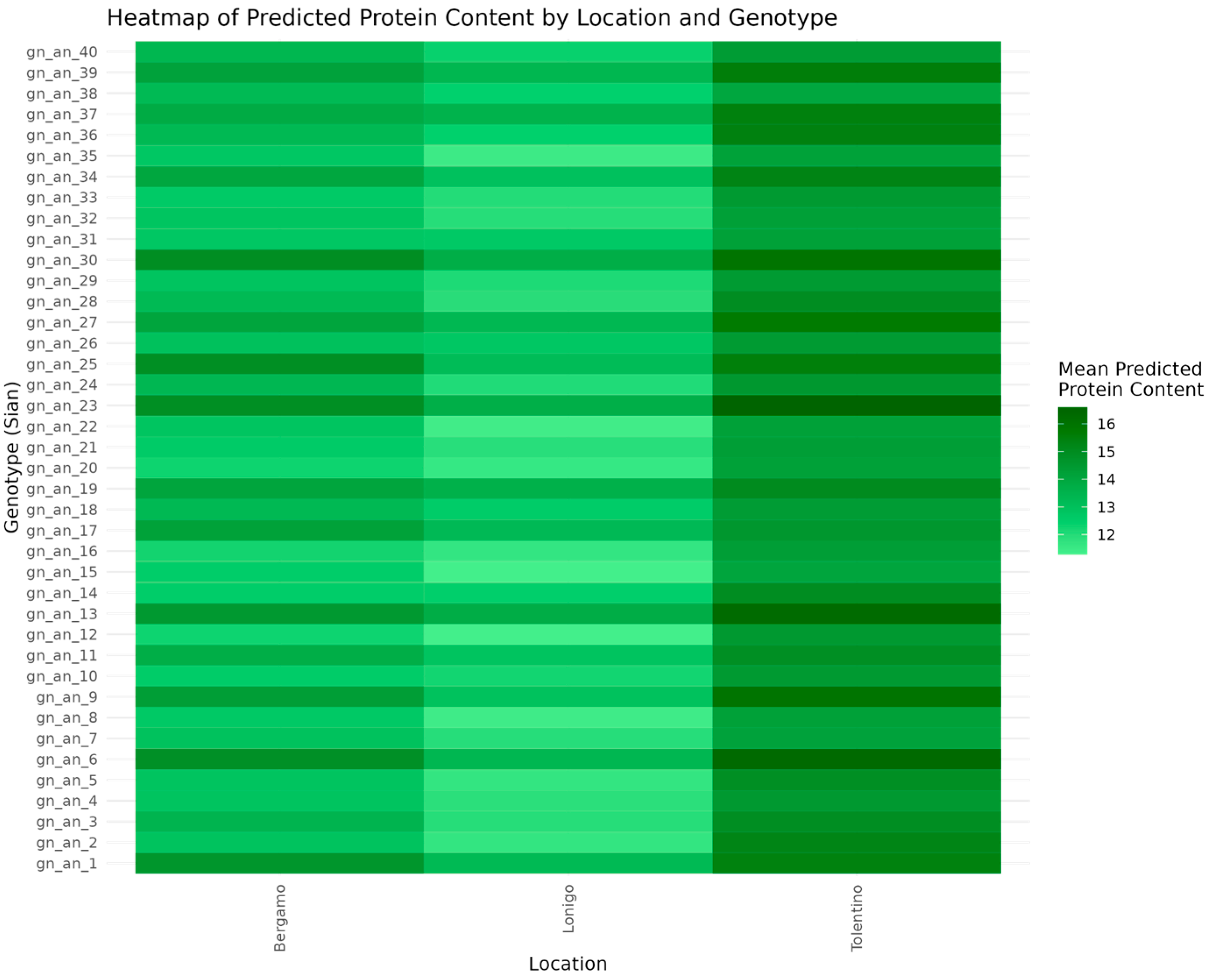
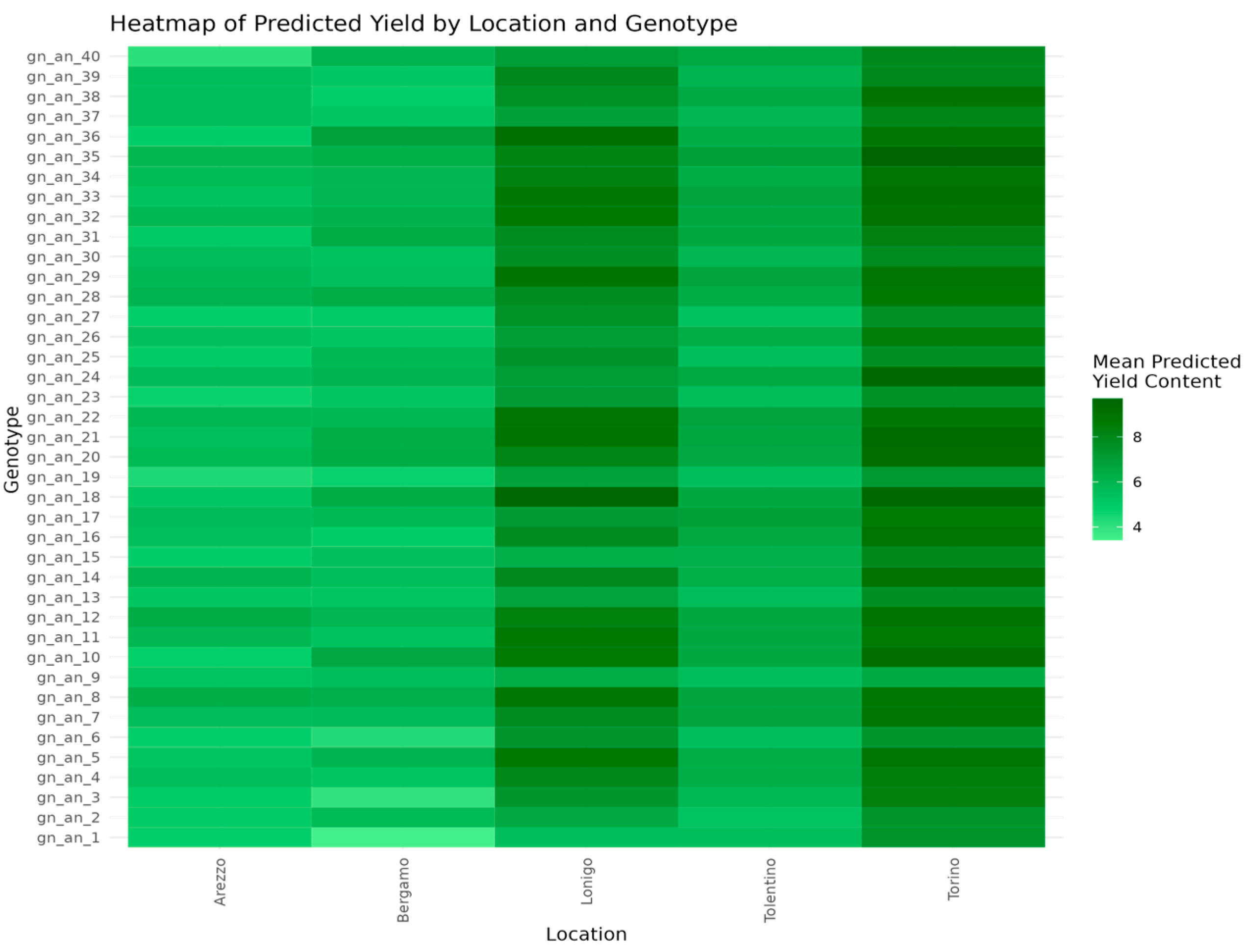
Explore temporal stability and environmental performance, highlighting consistently favorable sites such as Tolentino (protein) and Torino (yield);

(vi).

Demonstrate how the protocol can improve regulatory transparency, support agricultural innovation, and contribute to food security.

To introduce the general concepts of Interpretable Machine Learning (IML), we applied the Random Forest model to predict wheat cultivar yields and protein contents. To specifically address and illustrate Genotype-by-Environment (G×E) interactions within the IML framework, we employed AMBARTI—a model capable of capturing complex interaction patterns and producing intuitive visualizations [27]. The dataset used in this study—originating from Italian registration trials—enabled us to showcase AMBARTI’s communication value, particularly in highlighting key interactions that influence performance [28,29].

AMBARTI was selected for its ability to model G×E structures while generating interpretable results that go beyond traditional tools like biplots [27]. All methods described are fully reproducible using open-source tools in R, as detailed in the methodology section.

2. Materials and Methods

2.1. Experimental Design

The dataset used in this study comprises 40 anonymized wheat genotypes, including 36 new varieties and 4 reference varieties. Among the new varieties, 26 have been registered in the Italian Variety Catalogue. Genotype anonymization was carried out in two ways: (i) for the Random Forests application, genotypes were coded as gn_an_1 through gn_an_40; and, (ii) for the AMBARTI visualizations, genotypes were labeled as g1, g2, … g40, due to the software’s automatic anonymization feature [27].

These genotypes were evaluated for two key traits, yield (t/ha) and protein content (%), across different environmental conditions during the 2021 and 2022 seasons. Yield was assessed in five distinct environments, each corresponding to a different location (Arezzo, Bergamo, Lonigo, Tolentino, and Torino). For the Random Forests IML illustrations, original location names were retained. In the case of AMBARTI, environments were automatically coded as e1 through e5, as shown in

Table 1. Correspondence between the environments and its code for protein evaluations in Years 1 (2021) and 2 (2022) in the AMBARTI outputs.

Location	Code
Bergamo	e1
Lonigo	e2
Tolentino	e3

[27]. Yields were measured in tons per hectare under a standard grain humidity of 13.5%, providing a consistent basis for comparing productivity across environments.

Protein content was evaluated in three locations (Bergamo, Lonigo, and Tolentino), represented as e1 through e3 in

Table 2. Correspondence between the environments and its code for yield evaluations in Years 1 (2021) and 2 (2022) in the AMBARTI outputs.

Location	GPS Coordinates of Field Trials	Code
Arezzo	43.184500–11.494800	e1
Bergamo	45.661050–9.659516	e2
Lonigo	45.392700–11.380719	e3
Tolentino	13.346147–43.233995	e4
Torino	44.894023–7.878138	e5

. These evaluations allowed us to assess the nutritional quality of wheat genotypes across different conditions. Notably, the e1, e2, etc. labels differ between Table 1 and Table 2, as they correspond to different subsets of environments. This discrepancy stems from the AMBARTI software, which automatically assigns generic codes (g1, e1, etc.) without preserving consistent mapping across outputs [27]. All field trials followed a randomized complete block design with three replicates per environment.

For each location, the following weather variables, collected via NASAPOWER system, were considered: Temperature at 2 m (T2M–Celsius), Relative Humidity at 2 meters (RH2M—%), Corrected Total Precipitation (PRECTOTCORR—mm), Wind Speed at 2 meters (WS2M—m/s), and Ground Wetness Profile (GWETPROF—dimensionless). Each of the weather variables were collected daily, but, during the analysis, they were aggregated in the median values of the daily minimum, maximum, and quantile 0.05, 0.50, and 0.95 values.

Note on Environment Codes:

It is important to highlight that the codes used to represent environments (e.g., e1 to e5) when using the AMBARTI method differ between yield and protein content analyses due to the fact that each trait was assessed in a different subset of locations. These codes are automatically assigned by the modeling software R version 4.5.1 and serve only as internal categorical identifiers within each model. Since the environment variable is modeled as a categorical factor summarizing multiple underlying weather variables, these labels do not have intrinsic meaning across traits or figures and do not compromise the consistency or validity of interpretation within each modeling context.

2.2. Random Forests, Interpretable Machine Learning, Variable Importance, and Interactions

Random Forests (RF) [30] are ensemble learning models widely used for classification and regression. Their predictive robustness stems from aggregating multiple decision trees trained on bootstrap samples, with added randomness at each split to improve model generalization. For regression, RF outputs the average of tree predictions.

A major advantage of RF is its ability to estimate variable importance, typically using either Mean Decrease in Accuracy (MDA) or Mean Decrease in Gini (MDG) [25,26].

●

MDA evaluates how permuting a variable affects prediction accuracy:

$$\mathit{MDA}=\frac{1}{N}\ast \mathsf{\sum }(\mathit{Acc\_original}-\mathit{Acc\_permuted\_i})\mathit{for}i=1\mathit{to}N$$

MDG measures the cumulative reduction in impurity (e.g., Gini index) across all splits involving that variable:

$$\mathit{MDG}=\mathsf{\sum }\Delta \mathit{Gini}\left(t\right)\mathit{for}\mathit{all}t\mathit{in}\mathit{Trees}$$

RF also captures variable interactions, enabling the identification of predictor pairs that jointly influence the model’s response. These interactions are visualized using the vivid R package [25,26], which provides the following:

●

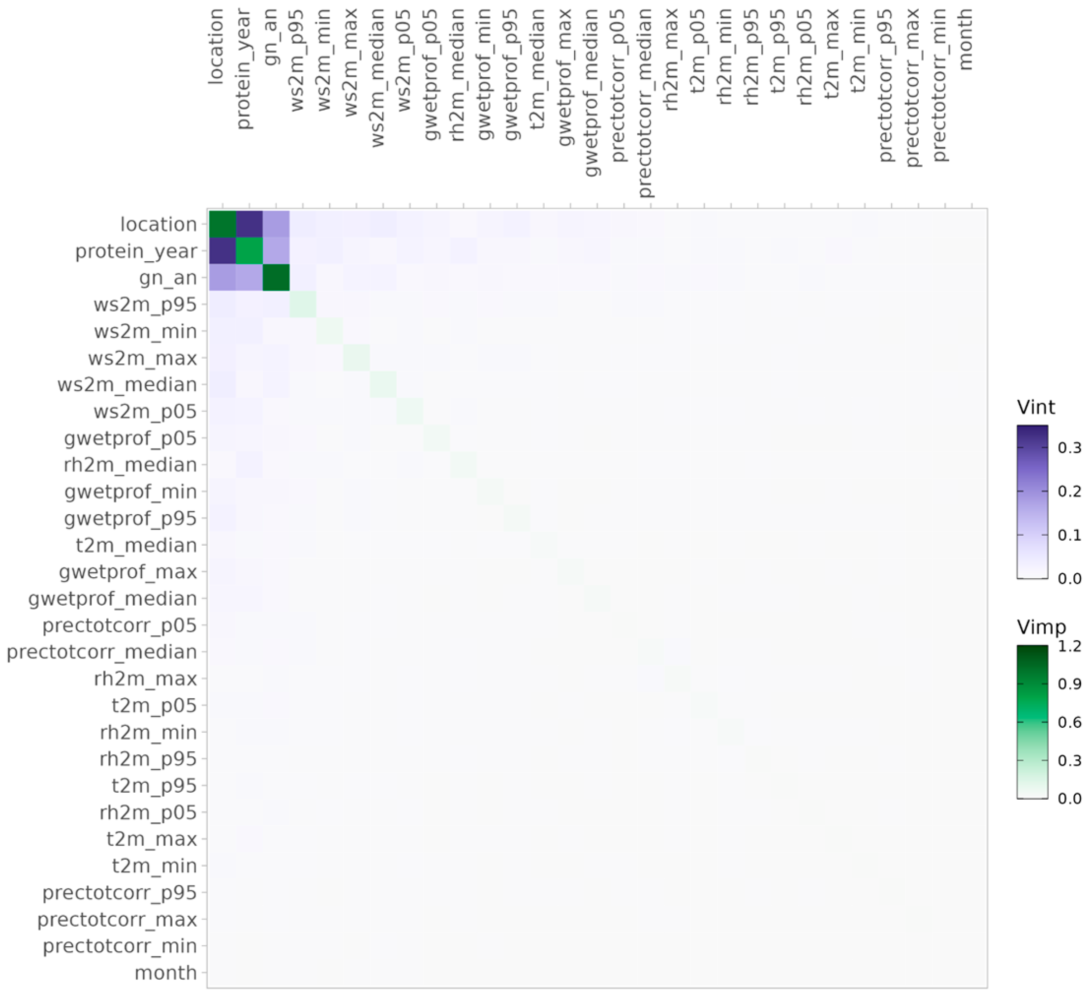
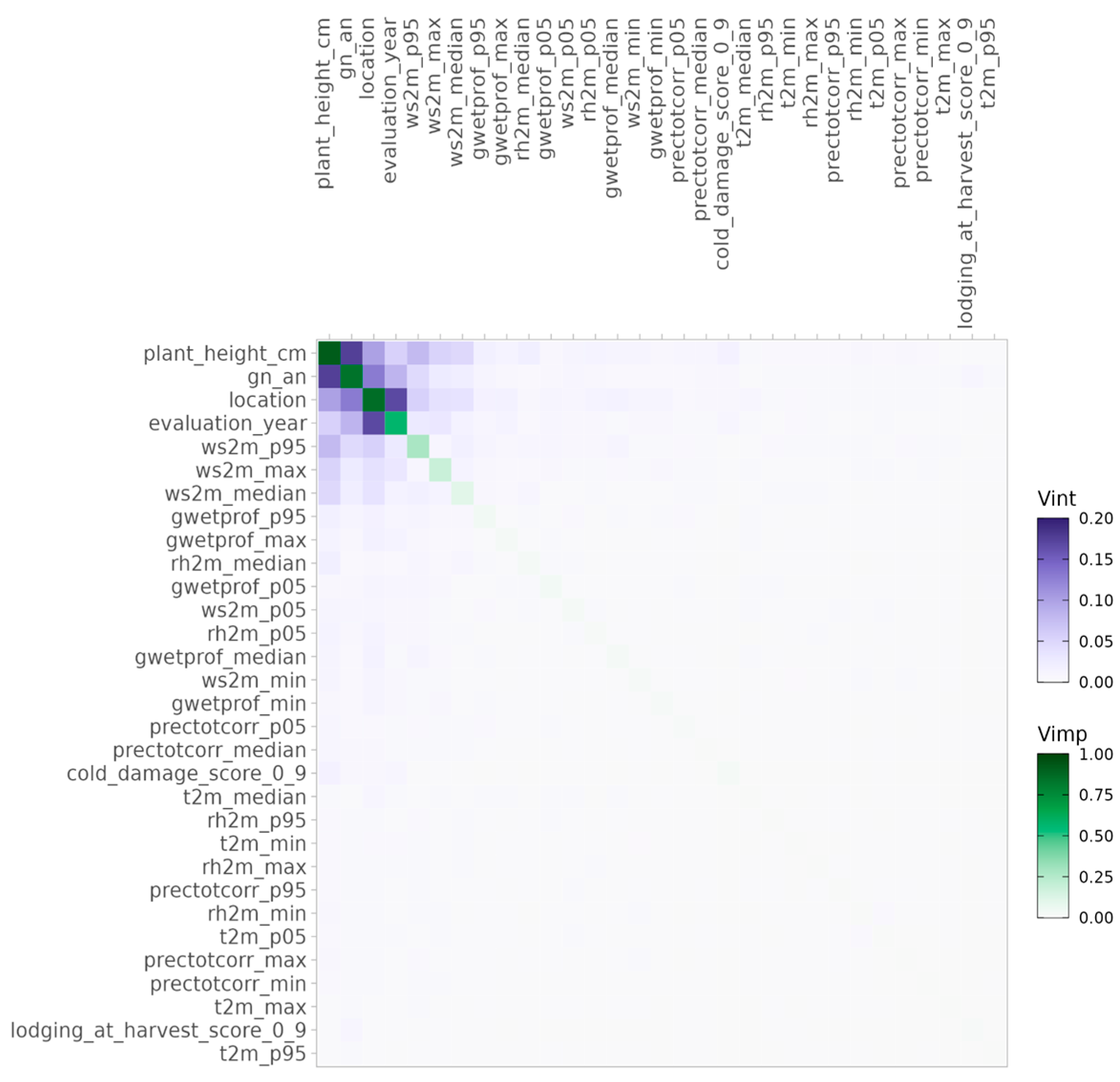
Heatmaps (viviHeatmap): These show variable importance on the diagonal and interactions on the off-diagonal;

●

Network graphs (viviNetwork): These represent variables as nodes, with node size and color indicating importance, and edge thickness reflecting interaction strength.

In this study, we used these visual tools to support communication within Variety Registration Offices (VROs), enabling clear interpretation of predictors and their interrelations from ML models. Additionally, the viviNetwork function was instrumental in visualizing variables as nodes within a network graph, where node size and color intensity reflected variable importance, and edge thickness indicated interaction strength. Advanced features such as filtering and clustering based on interaction strengths allowed for focused analysis on significant variables, enhancing the interpretability of the model’s predictions [25,26].

2.3. AMBARTI Method

To specifically model Genotype-by-Environment (G×E) interactions, we employed the AMBARTI method (Bayesian Additive Regression Trees for G×E interaction) [27]. This model decomposes phenotypic response into additive and interaction components:

$$p_{ij}=g_i+e_j+{(ge)}_{ij}$$

where p_ij is the response, g_i is the genotype effect, e_j the environment effect, and ge_ij the interaction term. AMBARTI modifies the BART model structure [31], extending it to G×E contexts using a Bayesian analogue of the AMMI model [28,32]. The predictive model is defined as follows:

$$\mathit{y\_ij}|\mathit{x\_ij},\mathsf{\Theta }\sim N(\mathsf{\mu }+\mathit{g\_i}+\mathit{e\_j}+\mathsf{\sum }(t=1\mathit{to}T)\mathit{of}h(\mathit{x\_ij},\mathit{M\_t},\mathit{T\_t}),{\sigma }^2)$$

In this equation, y_ij represents the response for genotype (i) and environment (j). The term Θ denotes the set of parameters (μ, g_i, e_j, M_t, T_t, σ²). Here, μ is the grand mean, and g_i and e_j are the effects of genotypes and environments, respectively. The term h (x_ij, M_t, T_t) represents a function applied to the genotype–environment combination, where M_t and T_t are model-specific parameters. The response follows a normal distribution with mean given by the sum of these effects and variance σ². Addressing the interactions using the tools presented in the AMBARTI Equation allows the user to address more complex mathematical structures in the interaction, which makes AMBARTI a better alternative when compared to the main models used in G by E studies, as shown in [27]. The method also allows for interpretable machine-learning solutions such as variable interactions and importance via heatmaps and bi-partite networks [25,26], making the visual outputs more efficient than traditional AMMI biplots in terms of communicating outputs of the model [27]. A comprehensive comparative analysis between AMBARTI and existing methods was presented in the original paper describing the method [27]. In that study, AMBARTI was benchmarked against the traditional AMMI model, and its Bayesian counterpart (B-AMMI), as well as more flexible interaction detection methods such as Smoothing Spline ANOVA (SS-ANOVA) and Bayesian Multivariate Adaptive Regression Splines (B-MARS). Simulation results revealed that, while AMMI performed well under bilinear interaction structures (its natural setting), it failed to capture the more complex interaction patterns simulated under AMBARTI [27]. Across multiple scenarios, AMBARTI demonstrated superior or highly competitive performance, particularly in predictive accuracy and in modeling non-additive, high-dimensional G×E structures. Furthermore, AMBARTI eliminated the need for pre-selecting the number of interaction components (as required in AMMI) and provided a posterior distribution for each parameter, enhancing uncertainty quantification [27]. It is important to note that the methods applied in this study—Random Forests and AMBARTI—do not rely on classical parametric inference procedures such as ANOVA or p-values. Instead, they offer alternative, model-based strategies to evaluate variable relevance and interaction strength. Random Forests derive variable importance and interaction metrics based on their contribution to prediction accuracy or reduction in node impurity. AMBARTI, as a Bayesian approach, provides posterior distributions and credible intervals for all components, enabling probabilistic reasoning and uncertainty quantification. These strategies are aligned with the principles of Interpretable Machine Learning, where the focus shifts from traditional hypothesis testing to model-based interpretation and visualization, especially in high-dimensional or complex settings like G×E trials. This shift enhances the ability of registration offices to communicate results transparently and support decision-making grounded in predictive relevance rather than statistical significance alone.

3. Results

3.1. Illustrating a Communication Protocol with IML Tools

In this section, we illustrate how Interpretable Machine-Learning (IML) techniques can be used to support and enhance communication strategies within Variety Registration Offices (VROs). Rather than comparing the predictive accuracy of models, our goal is to demonstrate a structured protocol that integrates visual and analytical tools derived from IML to inform variety approval decisions. We present results from two complementary models—Random Forests and AMBARTI—to showcase how variable importance, Genotype-by-Environment (G×E) interactions, and performance rankings can be translated into actionable visual summaries. The outputs are organized to reflect the steps of this proposed communication protocol: first, exploring predictions and variable effects using Random Forests; then, deepening G×E insights with the AMBARTI model; and, finally, synthesizing key findings into summary tools tailored to decision-makers.

3.2. Visualizing Trial Data with Random Forests

3.2.1. Protein Content Predictions for Communication (2021 and 2022)

We first explore the predicted protein content generated by the Random Forest model across the 2021 and 2022 trials using a heatmap (Figure 1). This visualization facilitates the identification of genotypes with a high performance or stable expression across three environments: Bergamo, Lonigo, and Torino. Notably, genotypes such as gn_an_39, gn_an_37, gn_an_36, gn_an_23, gn_an_13, gn_an_9, and gn_an_6 exhibit a superior protein content in Bergamo. Genotype gn_an_37 demonstrates a moderate protein content across all environments, representing a stable performer. Environments themselves can also be ranked from this heatmap, with Torino and Lonigo generally showing higher protein predictions. These insights serve as an example of how such visualizations can enhance internal VRO communication, support environmental targeting, and assist breeding decisions.

3.2.2. Identifying Key Variables and Interactions for Protein

To explore the main drivers of protein predictions, we display the variable importance and interaction in Figure 2. The location, year (protein_year), and genotype are the most important predictors, while interactions between gwetprof_p95 and prectotcorr_min are prominent, indicating a synergy between soil wetness and precipitation. A complementary visualization is provided in Figure 3, showing the same structure as a network.

3.2.3. Yield Predictions and Genotypic Stability

Figure 4 displays the predicted yield across genotypes and environments, revealing high-yielding performers like gn_an_12 (Arezzo), gn_an_24 (Torino), and gn_an_36 (Bergamo). Conversely, gn_an_9 and gn_an_19 underperform in Torino. Some genotypes, like gn_an_40, maintain a stable yield across all environments. These patterns provide intuitive guidance to registration offices and demonstrate the ability of heatmaps to communicate stability vs. sensitivity clearly.

The variable importance and interaction heatmaps for yield (Figure 5) identify the location, evaluation_year, plant height, and genotype as critical predictors. Their interactions are visualized via a network (Figure 6), emphasizing the role of ws2m_max, rh2m_median, and gwetprof_p95 as key environmental variables affecting yield.

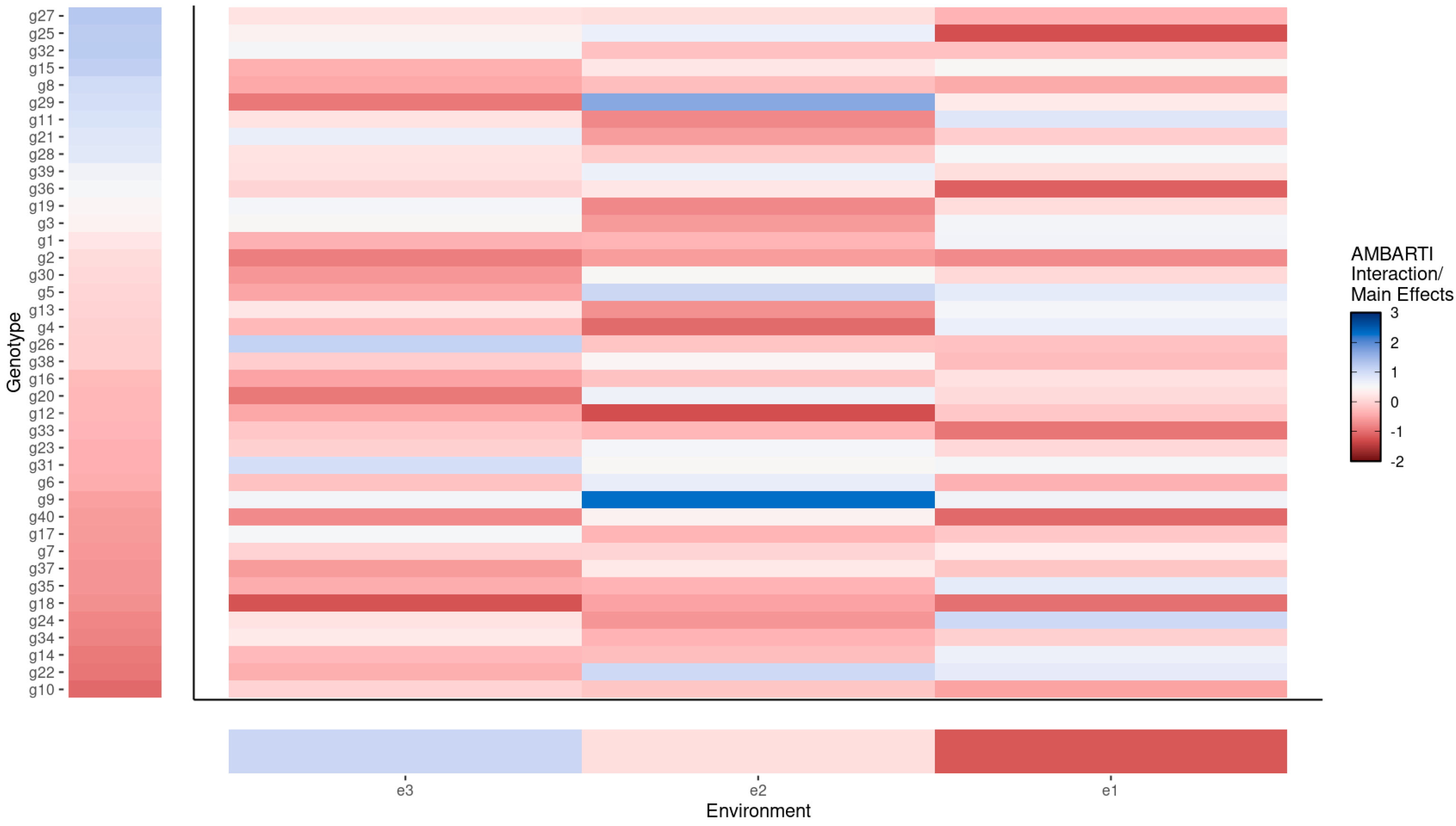
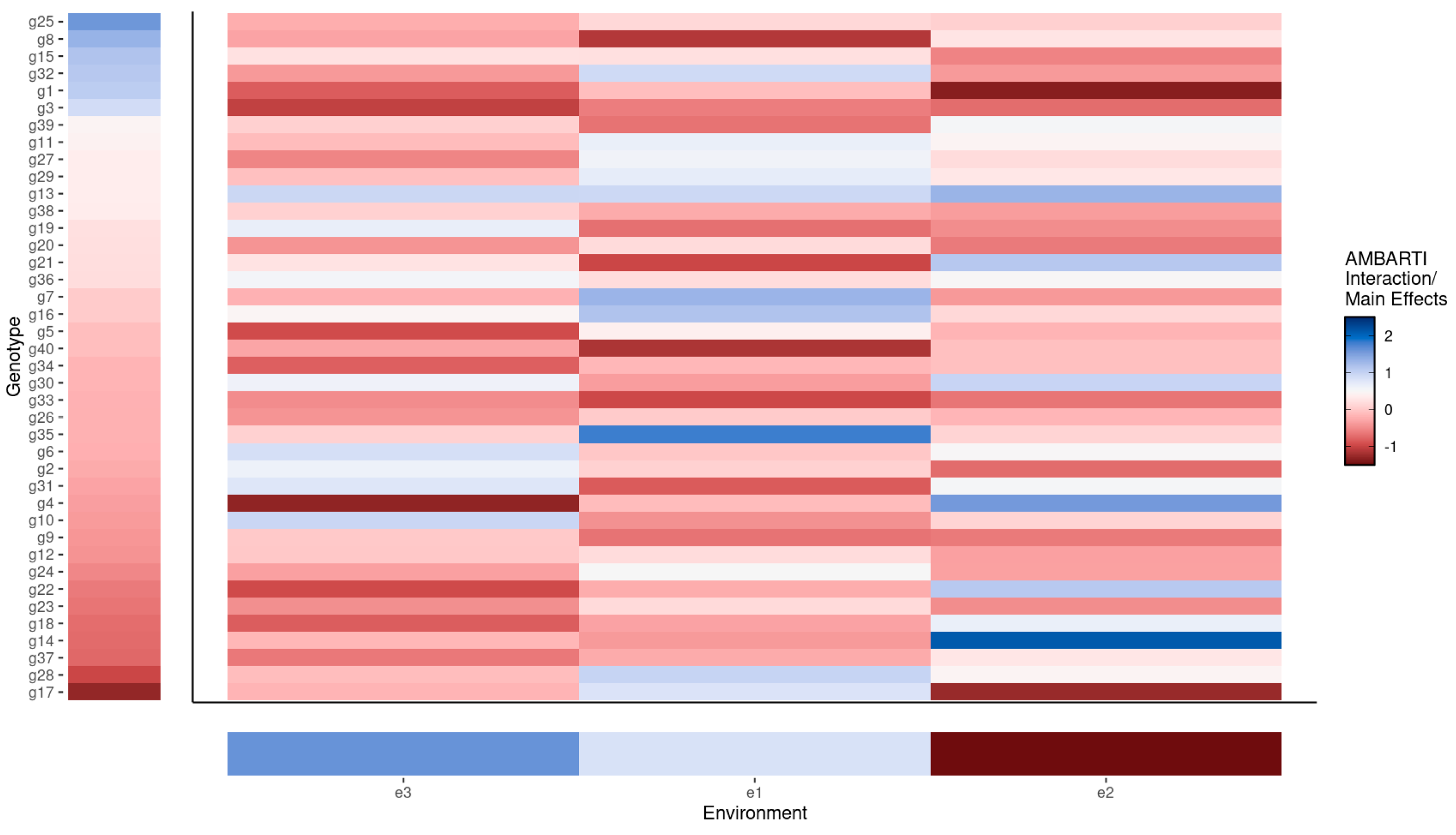
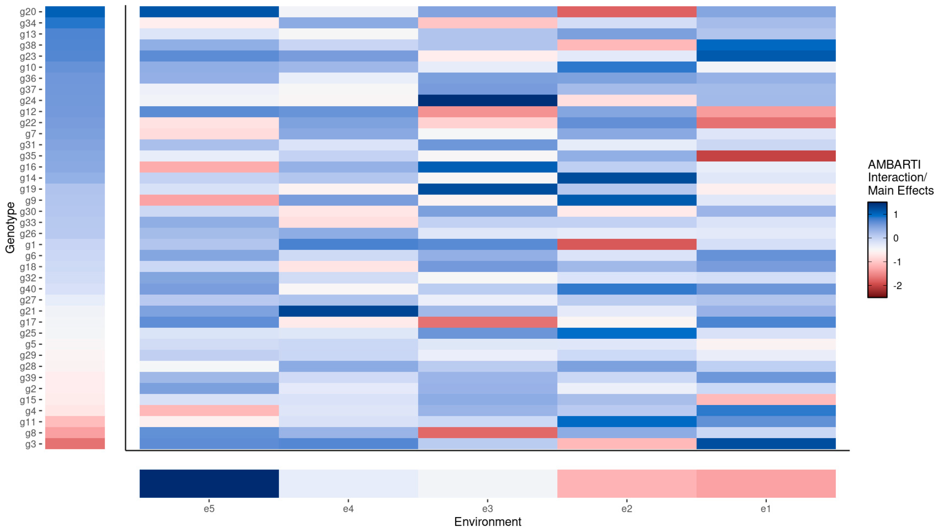
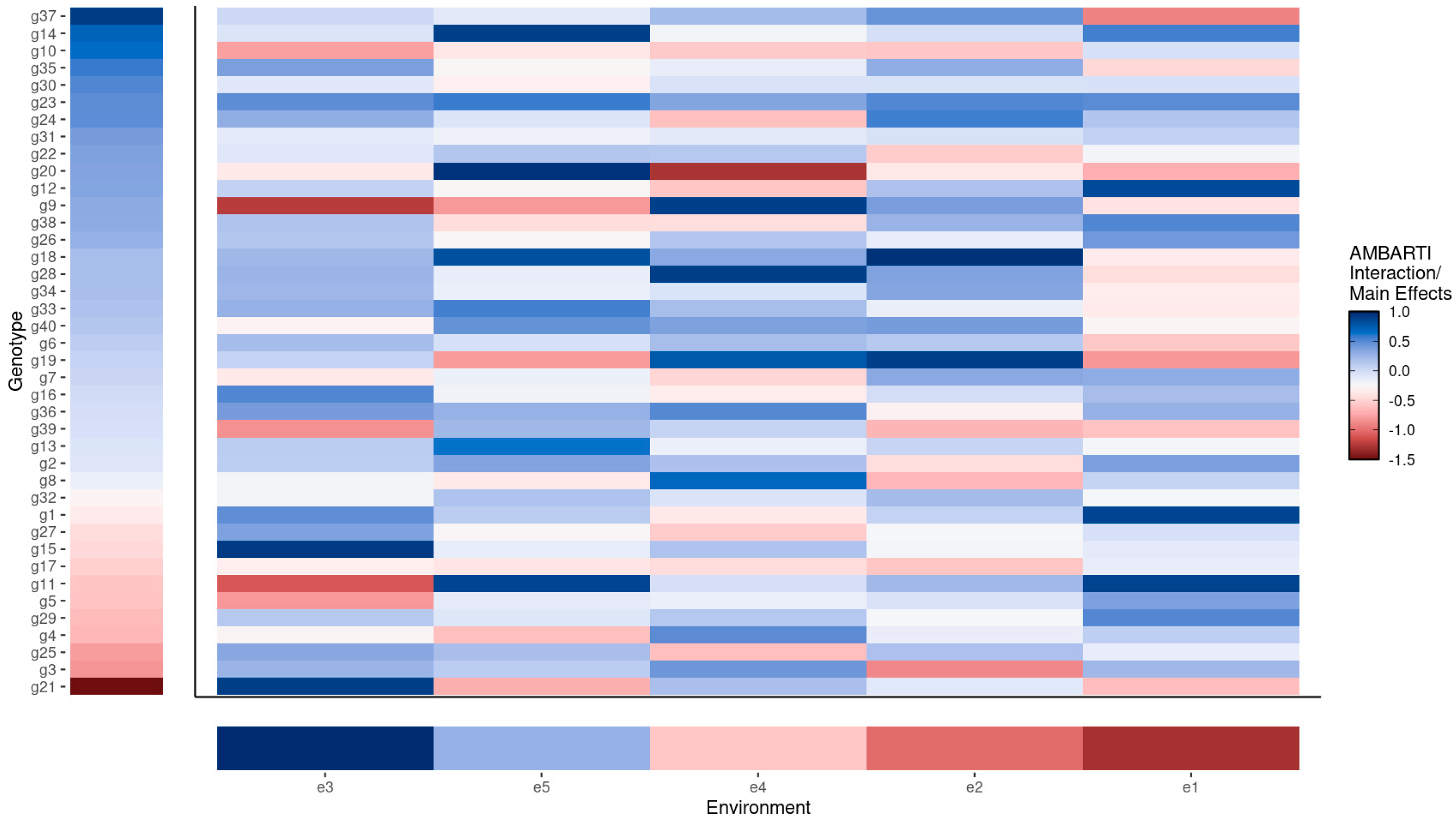
3.3. Visual Summaries via AMBARTI for G×E Understanding

3.3.1. Mapping Protein and Yield Interactions

Figure 7, Figure 8, Figure 9 and Figure 10 illustrate the G×E interactions and main effects from AMBARTI models for yield and protein across both years. These heatmaps reveal how genotypic performance and environment rankings change over time. For protein, e3 ranks the highest in both years. Genotype g25 maintains top ranking across both years, while g27 drops substantially.

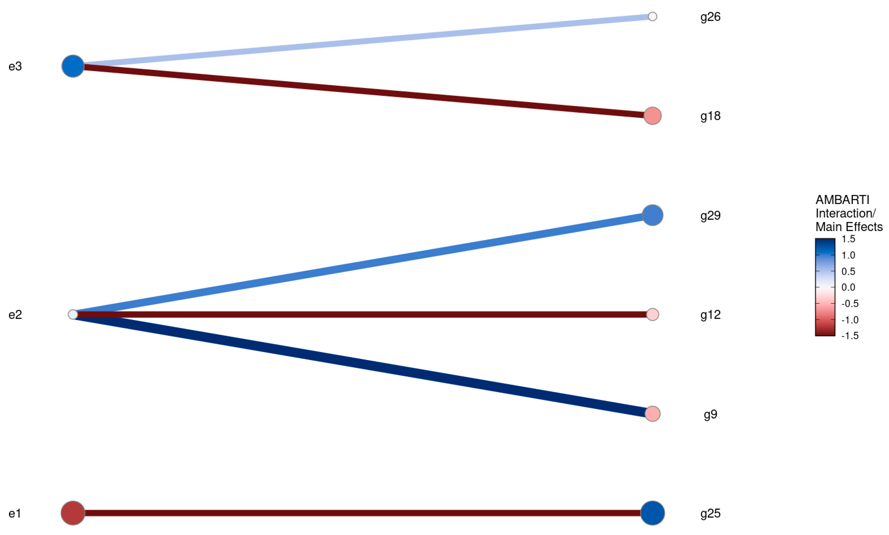
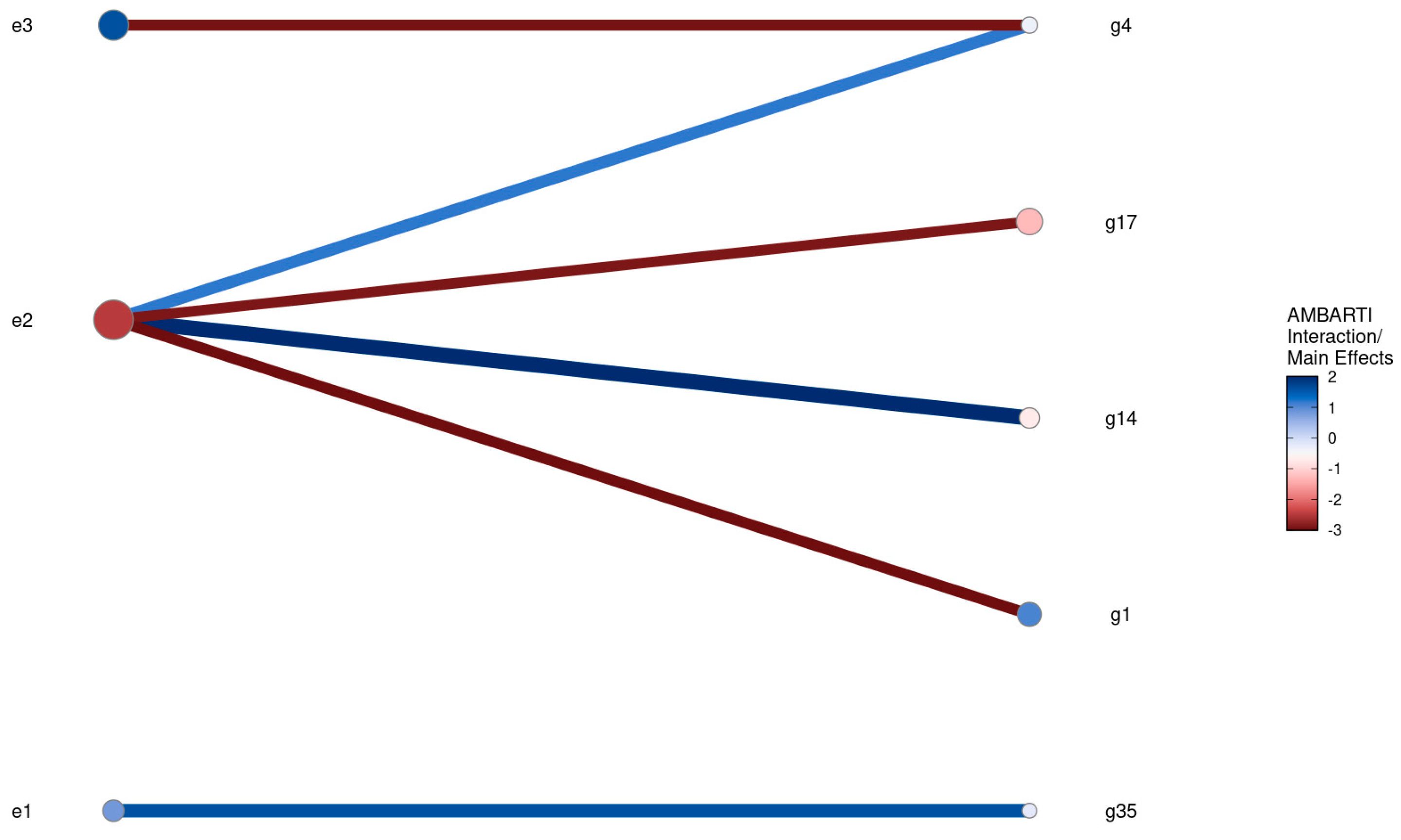
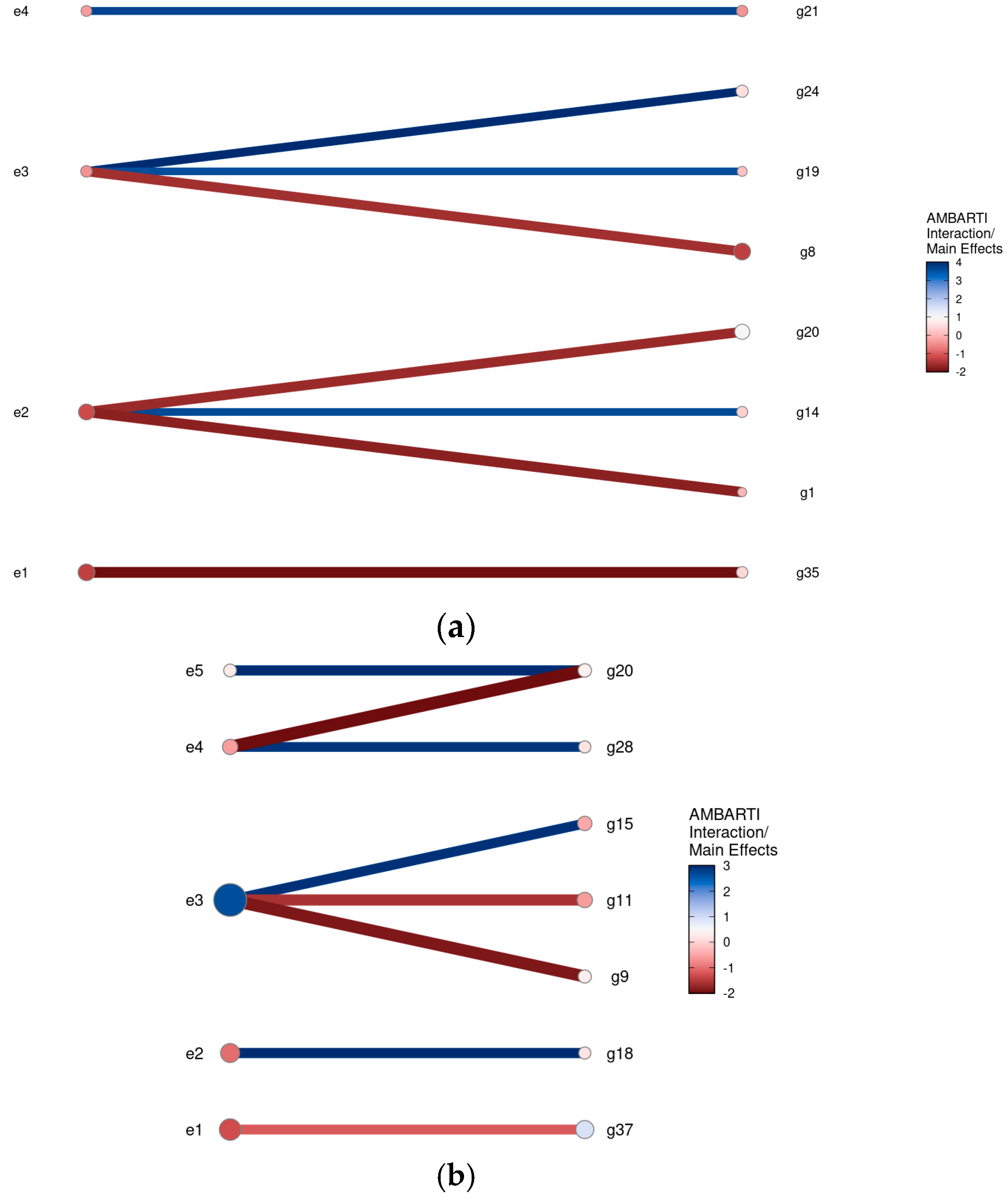
3.3.2. Highlighting Extreme Interactions via Networks

Figure 11 and Figure 12 display bipartite networks illustrating the top 2% strongest positive and negative G×E interactions. For instance, in protein data for year one, environment e3 interacts positively with g26 and negatively with g18. This network-based visualization supports the fast identification of critical genotype–environment matches.

3.3.3. Synthesizing Genotype and Environment Rankings

Table 3. Rank of environments in terms of protein and yield over the two years evaluated. Rank 1 implies the best environment in the set of environments considered (AMBARTI analysis).

Rank	Rank_Protein_Year1	Rank_Protein_Year2	Rank_Yield_Year1	Rank_Yield_Year2
1	Tolentino	Lonigo	Torino	Torino
2	Lonigo	Tolentino	Toentino	Tolentino
3	Bergamo	Bergamo	Lonigo	Arezzo
4			Bergamo	Lonigo
5			Arezzo	Bergamo

and

Table 4. Rank of genotypes in terms of protein and yield over the two years evaluated with AMBARTI method. Rank 1 implies the best genotype in the set of genotypes considered.

Genotype	Rank Prot Year 1	Rank Prot Year 2	Rank Yld Year 1	Rank Yld Year 2
g1	14	5	22	30
g10	40	30	6	3
g11	7	8	38	34
g12	24	32	10	11
g13	18	11	3	26
g14	38	37	16	2
g15	4	3	36	32
g16	22	18	15	23
g17	31	40	29	33
g18	35	36	24	15
g19	12	13	17	21
g2	15	27	35	27
g20	23	14	1	10
g21	8	15	28	40
g22	39	34	11	9
g23	26	35	5	6
g24	36	33	9	7
g25	2	1	30	38
g26	20	24	21	14
g27	1	9	27	31
g28	9	39	33	16
g29	6	10	32	36
g3	13	6	40	39
g30	16	22	19	5
g31	27	28	13	8
g32	3	4	25	29
g33	25	23	20	18
g34	37	21	2	17
g35	34	25	14	4
g36	11	16	7	24
g37	33	38	8	1
g38	21	12	4	13
g39	10	7	34	25
g4	19	29	37	37
g40	30	20	26	19
g5	17	19	31	35
g6	28	26	23	20
g7	32	17	12	22
g8	5	2	39	28
g9	29	31	18	12

summarize the environment and genotype ranks for both traits across two years. These rankings help structure VRO decisions regarding stability, performance, and temporal consistency.

3.4. Proposed Four-Step Protocol for IML-Based Communication in Variety Registration

Based on our results, we propose a four-step protocol:

1. Model fitting and visualization: Fit a model that allows for IML techniques, in our case, Random Forest or AMBARTI, to generate heatmaps and network plots (Figure 1, Figure 2, Figure 3, Figure 4, Figure 5 and Figure 6).

2. Identification of stable performers: Use visual summaries to identify stable genotypes (Figure 4 and Figure 7, Figure 8, Figure 9 and Figure 10).

3. Environmental matching: Analyze the importance of environmental drivers (Figure 2 and Figure 5) and interactions.

4. Communication and decision support: Translate findings into visual summaries and rankings (Table 3 and Table 4; Figure 11 and Figure 12) for evidence-based decisions.

4. Discussion

4.1. Enhancing Communication with IML Visual Tools

The results demonstrate that IML visualizations such as heatmaps and network plots can substantially improve communication within and beyond Variety Registration Offices (VROs). For example, the heatmaps in Figure 1 and Figure 4 allow for the immediate identification of genotypes with a high protein content or yield across multiple environments. The color gradients help non-specialists interpret performance levels without needing technical training in statistical modeling. Similarly, the importance–interaction heatmaps (Figure 2 and Figure 5) and their network counterparts (Figure 3 and Figure 6) provide accessible summaries of key predictors and their interactions. These tools support both internal technical decisions—such as genotype selection—and external communication with stakeholders, including farmers and breeders. The bipartite graphs from AMBARTI (Figure 11 and Figure 12) go a step further by visually highlighting the strongest 2% of positive and negative Genotype-by-Environment (G×E) interactions. These graphical interfaces simplify the translation of complex model outputs into intuitive, action-oriented insights that can be shared across interdisciplinary teams and institutional levels.

4.2. From Predictions to Practice: Translating Model Outputs

Beyond visual appeal, the results offer actionable insights. In the Random Forest model, certain genotypes such as gn_an_36, gn_an_12, and gn_an_40 demonstrated either a high yield or stable performance across environments, while others (e.g., gn_an_18) showed strong environmental responsiveness. Likewise, genotypes like g25, g32, and g8 consistently ranked among the top for protein content in the AMBARTI model, despite shifts in environmental rankings between years. These patterns can inform concrete recommendations for variety approval, regional planting advisories, or even strategic breeding focus areas. Additionally, the identification of environmental covariates—such as gwetprof_p95, ws2m_max, and rh2m_median—as key predictors allows VROs to better explain why certain genotypes succeed or fail in specific contexts. This level of detail strengthens the practical value of variety assessments, grounding them in observable, climate-linked drivers rather than opaque statistical models.

4.3. Stability vs. Responsiveness: A Visual Dialogue

The analysis also revealed the dual importance of identifying both stable and responsive genotypes. For example, genotype gn_an_37 consistently presented a moderate protein content across sites, while gn_an_12 and gn_an_36 exhibited a high yield in specific environments. The capacity to visually differentiate such patterns—via color saturation or interaction strength—enables VROs to simultaneously support breeding for stability and breeding for responsiveness, depending on the policy or market needs. In AMBARTI’s bipartite networks, we observe genotypes such as g27 dropping from first to ninth place over two years, illustrating a sensitivity to environmental shifts. Meanwhile, genotype g25 rose from second to first, signaling robustness. By visually encoding this type of temporal and environmental variability, IML tools offer a compelling narrative that can be shared in technical reports or farmer guides, enhancing the clarity of public-facing recommendations.

4.4. Proposed Protocol for IML-Based Communication

Building on the empirical results, we propose a four-step protocol to guide the use of IML tools in VRO workflows:

1. Model fitting and visualization: Employ Random Forests or AMBARTI to model G×E interactions and generate interpretable visual summaries, such as heatmaps of variable importance and interaction strength (Figure 2 and Figure 5).

2. Identification of stable performers: Use network representations (e.g., Figure 3) and G×E bipartite graphs (Figure 11 and Figure 12) to flag genotypes with consistently high or robust performance.

3. Environmental matching: Examine which environmental covariates most influence genotype success (e.g., wind speed, humidity, and soil moisture) and leverage those to explain variety behavior across agro-climatic zones.

4. Communication and decision support: Translate the results into accessible tools—such as recommendation maps or summary tables (Table 3 and Table 4)—to support variety approvals and stakeholder engagement.

This protocol promotes transparency and reduces the reliance on arbitrary thresholds, replacing them with evidence-based criteria drawn directly from model interpretation. It also bridges the gap between data science and regulatory practice, aligning model outputs with the real needs of public agencies, breeders, and growers.

4.5. Final Remarks: Moving Beyond Predictive Accuracy

It is important to emphasize that the primary aim of this paper is not to compare or identify the most accurate predictive model. Instead, our focus lies in proposing and demonstrating a practical, interpretable framework for improving institutional communication in variety registration workflows. By using Random Forests and AMBARTI as illustrative models, we highlight how Interpretable Machine-Learning (IML) tools—such as heatmaps, interaction plots, and bipartite networks—can be integrated into a transparent and replicable communication protocol. We acknowledge that a more in-depth comparison of modeling approaches—including the use of multiple feature selection strategies—can offer valuable insights. For instance, future studies dedicated to modeling performance could explore a range of feature selection techniques, starting with filter methods such as RReliefF to assess individual variable importance, followed by wrapper methods like Recursive Feature Elimination or Exhaustive Feature Selection to evaluate variable combinations. Comparing these methods alongside predictive performance metrics would provide a more comprehensive modeling assessment. However, such analyses go beyond the scope of the current study, whose goal is not to benchmark models but to showcase how IML tools can enhance the interpretability and communicability of model outputs within regulatory environments. We encourage future work to expand on this direction by systematically exploring model selection, tuning, and feature reduction strategies in the context of high-dimensional Genotype-by-Environment data.

5. Conclusions

This study underscores the critical role that Interpretable Machine-Learning (IML) [9] tools can play in enhancing the communication strategies of Variety Registration Offices (VROs) [10,33] through the use of intuitive visual techniques. By applying Random Forests and AMBARTI models, we were able to dissect and present complex Genotype-by-Environment (G×E) interactions in an accessible and interpretable way. The visual outputs generated by these models—such as heatmaps and network plots—serve not merely as analytical results but as communication bridges, translating complex, multidimensional data into formats that are easily understood. These visualizations enable VROs to effectively convey the nuanced effects of environmental factors on wheat yield and protein content. The integration of IML tools, particularly their visual components, provides VROs with a distinct advantage. They support objective, data-driven decision-making by clearly illustrating variable importance and interactions, thereby simplifying otherwise complex evaluations. The graphical representation of G×E interactions has proven especially valuable for highlighting genotype stability and adaptability across diverse environmental conditions. This level of clarity enhances the alignment between breeding strategies and environmental realities, while also facilitating the communication of complex findings to broader audiences, including farmers and policymakers. Ultimately, these IML tools have the potential to transform the analysis and dissemination of agricultural data, paving the way for more informed crop selection and a more resilient approach to food production.

As a recommendation for future research, to deepen the understanding of how individual environmental and genotypic variables influence yield and protein content, future research could integrate advanced visualization techniques such as Partial Dependence Plots (PDPs), Accumulated Local Effects (ALE), or Individual Conditional Expectation (ICE) plots. These methods allow for a more granular interpretation of the marginal effects of specific predictors, particularly in non-linear models like Random Forests. By isolating the contribution of variables such as gwetprof_p95 (subsurface soil moisture), ws2m_max (maximum wind speed), and rh2m_median (relative humidity), these tools can uncover nuanced response patterns that are not immediately visible through global importance metrics alone. Incorporating such approaches would enhance the explanatory power of IML tools in the context of agricultural decision-making and could support more precise agronomic recommendations under varying climatic conditions. To further enhance the interpretability and robustness of predictive models in variety testing, future research could benefit from the incorporation of additional feature selection strategies beyond the embedded importance measures used in Random Forests. Filter methods such as RReliefF can help evaluate the individual relevance of predictors, while wrapper methods like Recursive Feature Elimination or Exhaustive Feature Selection allow the assessment of variable subsets in terms of predictive power. Employing a combination of these approaches would enable a more comprehensive understanding of which environmental and phenotypic factors most consistently influence yield and protein outcomes, offering a stronger foundation for model refinement and communication in regulatory contexts.

References

1. Ortiz, R. Role of plant breeding to sustain food security under climate change. In Food Security and Climate Change; John Wiley & Sons, Ltd.: Hoboken, NJ, USA, 2018; pp. 145–158. [Google Scholar] [CrossRef]
2. Wardofa, G.A.; Mohammed, H.; Asnake, D.; Alemu, T. Genotype x environment interaction and yield stability of bread wheat genotypes in Central Ethiopia. J. Plant Breed. Genet. 2019, 7, 87–94. [Google Scholar] [CrossRef]
3. Pour-Aboughadareh, A.; Khalili, M.; Poczai, P.; Olivoto, T. Stability indices to deciphering the genotype-by-environment interaction (GEI) effect: An applicable review for use in plant breeding programs. Plants 2022, 11, 414. [Google Scholar] [CrossRef] [PubMed]
4. Hamidi, A.; Ramezani Moghaddam, M.R.; Najjar, H.; Arab Salmani, M.; Mohajer Abbasi, A. Value of Cultivation and Use (VCU) Evaluation of Some New Promising Genotypes of Upland Cotton (Gossypium hisutum L.) in Razavi Khorasan Province. Agrotech. Ind. Crops 2022, 2, 166–176. [Google Scholar] [CrossRef]
5. Bozzoli, M. GWAS Analysis for the Identification of Molecular Basis Responsible for Yield-Related Traits and Disease Resistance in Durum Wheat. Ph.D. Thesis, University of Bologna, Bologna, Italy, 2023. [Google Scholar]
6. Wang, L.; Zheng, Y.; Duan, L.; Wang, M.; Wang, H.; Li, H.; Li, R.; Zhang, H. Artificial selection trend of wheat varieties released in Huang-Huai-Hai region in China evaluated using DUS testing characteristics. Front. Plant Sci. 2022, 13, 898102. [Google Scholar] [CrossRef] [PubMed]
7. Banjarey, P.; Rani, A.; Pandey, S.; Shukla, R.S.; Kumawat, S.; Singh, S. Morphological characterization of cms based wheat hybrids (Triticum aestivum L.). Int. J. Chem. Stud. 2022, 11, 172–175. [Google Scholar]
8. Ghimire, S.; Verdonk, T. International Conference--IP Protection for Plant Innovation 2021. GRUR Int. 2022, 71, 535–539. [Google Scholar] [CrossRef]
9. Sarti, D.; Wagner, J.; Palma, F.; Kalvan, H.; Giachini, M.; Lautenschalaeger, D.; Lupianhez, V.; Pires, J.; Sales, M.; Faria, P.; et al. Interpretable machine learning unveils key predictors and default values in an expanded database of human in vitro dermal absorption studies with pesticides. Regul. Toxicol. Pharmacol. 2025, 159, 105801. [Google Scholar] [CrossRef] [PubMed]
10. van Etten, J.; de Sousa, K.; Aguilar, A.; Barrios, M.; Coto, A.; Dell’Acqua, M.; Fadda, C.; Vicente, J.; Mina, D.; Steinke, J.; et al. Crop variety management for climate adaptation supported by citizen science. Proc. Natl. Acad. Sci. USA 2019, 116, 4194–4199. [Google Scholar] [CrossRef]
11. Nehe, A.; Akin, B.; Sanal, T.; Evlice, A.K.; Ünsal, R.; Dinçer, N.; Demir, L.; Geren, H.; Sevim, I.; Orhan, Ş. Genotype x environment interaction and genetic gain for grain yield and grain quality traits in Turkish spring wheat released between 1964 and 2010. PLoS ONE 2019, 14, e0219432. [Google Scholar] [CrossRef]
12. Ahakpaz, F.; Abdi, H.; Neyestani, E.; Hesami, A.; Mohammadi, B.; Mahmoudi, K.N.; Abedi-Asl, G.; Noshabadi, M.R.J.; Ahakpaz, F.; Alipour, H. Genotype-by-environment interaction analysis for grain yield of barley genotypes under dryland conditions and the role of monthly rainfall. Agric. Water Manag. 2021, 245, 106665. [Google Scholar] [CrossRef]
13. Gupta, V.; Kumar, M.; Singh, V.; Chaudhary, L.; Yashveer, S.; Sheoran, R.; Dalal, M.S.; Nain, A.; Lamba, K.; Gangadharaiah, N. Genotype by environment interaction analysis for grain yield of wheat (Triticum aestivum (L.) em. Thell) genotypes. Agriculture 2022, 12, 1002. [Google Scholar] [CrossRef]
14. Benos, L.; Tagarakis, A.C.; Dolias, G.; Berruto, R.; Kateris, D.; Bochtis, D. Machine learning in agriculture: A comprehensive updated review. Sensors 2021, 21, 3758. [Google Scholar] [CrossRef] [PubMed]
15. Paudel, D.; Boogaard, H.; de Wit, A.; Janssen, S.; Osinga, S.; Pylianidis, C.; Athanasiadis, I.N. Machine learning for large-scale crop yield forecasting. Agric. Syst. 2021, 187, 103016. [Google Scholar] [CrossRef]
16. Zednik, C. Solving the black box problem: A normative framework for explainable artificial intelligence. Philos. Technol. 2021, 34, 265–288. [Google Scholar] [CrossRef]
17. Molnar, C.; Casalicchio, G.; Bischl, B. Interpretable machine learning—A brief history, state-of-the-art and challenges. In Joint European Conference on Machine Learning and Knowledge Discovery in Databases; Springer: Berlin/Heidelberg, Germany, 2020; pp. 417–431. [Google Scholar]
18. Rudin, C.; Chen, C.; Chen, Z.; Huang, H.; Semenova, L.; Zhong, C. Interpretable machine learning: Fundamental principles and 10 grand challenges. Stat. Surv. 2022, 16, 1–85. [Google Scholar] [CrossRef]
19. Carter, A.; Imtiaz, S.; Naterer, G.F. Review of interpretable machine learning for process industries. Process Saf. Environ. Prot. 2023, 170, 647–659. [Google Scholar] [CrossRef]
20. Chen, Y.; Calabrese, R.; Martin-Barragan, B. Interpretable machine learning for imbalanced credit scoring datasets. Eur. J. Oper. Res. 2024, 312, 357–372. [Google Scholar] [CrossRef]
21. Liu, B.; Lu, W.; Olofsson, T.; Zhuang, X.; Rabczuk, T. Stochastic interpretable machine learning-based multiscale modeling in thermal conductivity of Polymeric graphene-enhanced composites. Compos. Struct. 2024, 327, 117601. [Google Scholar] [CrossRef]
22. Lee, M.-H. Predicting and analyzing the fill factor of non-fullerene organic solar cells based on material properties and interpretable machine-learning strategies. Sol. Energy 2024, 267, 112191. [Google Scholar] [CrossRef]
23. Zhou, M.; Li, Y. Spatial distribution and source identification of potentially toxic elements in Yellow River Delta soils, China: An interpretable machine-learning approach. Sci. Total Environ. 2024, 912, 169092. [Google Scholar] [CrossRef]
24. Wani, N.A.; Kumar, R.; Bedi, J. DeepXplainer: An interpretable deep learning-based approach for lung cancer detection using explainable artificial intelligence. Comput. Methods Programs Biomed. 2024, 243, 107879. [Google Scholar] [CrossRef] [PubMed]
25. Inglis, A.; Parnell, A. Vivid: An R package for Variable Importance and Variable Interactions Displays for Machine Learning Models. arXiv 2022, arXiv:2210.11391. [Google Scholar] [CrossRef]
26. Inglis, A.; Parnell, A.; Hurley, C.B. Visualizing variable importance and variable interaction effects in machine learning models. J. Comput. Graph. Stat. 2022, 31, 766–778. [Google Scholar] [CrossRef]
27. Sarti, D.A.; Prado, E.B.; Inglis, A.N.; Dos Santos, A.A.L.; Hurley, C.B.; Moral, R.A.; Parnell, A.C. Bayesian Additive Regression Trees for Genotype by Environment Interaction Models. Ann. Appl. Stat. 2023, 7, 1936–1957. [Google Scholar] [CrossRef]
28. Sarti, D.A. The Statistical Paradigm: Probabilistic and Multivariate Analysis Applied Through Computational Stimulation in the Interaction Between Genotype x Environment. Ph.D. Thesis, Universidade de Sao Paulo, Sao Paulo, Brazil, 2019. [Google Scholar]
29. Sarti, D.A.; Dias, C.T.S. Comparison between AMMI, W-AMMI and GGE methodology in the context of simulated data. Rev. Bras. de Biom. 2020, 38, 290–393. [Google Scholar] [CrossRef]
30. Genuer, R.; Poggi, J.M. Random Forests; Springer: Berlin/Heidelberg, Germany, 2020. [Google Scholar]
31. Chipman, H.A.; George, E.I.; McCulloch, R.E. BART: Bayesian additive regression trees. Ann. Appl. Stat. 2010, 4, 266–298. [Google Scholar] [CrossRef]
32. Josse, J.; van Eeuwijk, F.; Piepho, H.P.; Denis, J.B. Another look at Bayesian analysis of AMMI models for genotype-environment data. J. Agric. Biol. Environ. Stat. 2014, 19, 240–257. [Google Scholar] [CrossRef]
33. Brown, D.; van den Bergh, I.; de Bruin, S.; Machida, L.; van Etten, J. Data synthesis for crop variety evaluation. A review. Agron. Sustain. Dev. 2020, 40, 25. [Google Scholar] [CrossRef]
Figure 1. Heatmap of predicted protein content across genotypes and conditions considering 2021 and 2022. Predicted protein content for a range of genotypes subjected to conditions represented by three distinct locations: Bergamo, Lonigo, and Torino. Darker shades correspond to higher protein predictions, revealing the influence of genotype–environment interactions on protein expression. The analysis provides insights into the genotypes’ adaptability and potential for protein yield optimization in varying environmental contexts. Random Forests analysis comprises a simple tool to inform varieties performance.
Agronomy 15 01603 g001
Figure 2. Variable importance and interaction heatmap. Simple manner to show in a single plot variable interactions and importance obtained with Random Forests for protein content and weather variables considered. Location, year of evaluation (protein_year), and genotype levels arise as more important variables.
Agronomy 15 01603 g002
Figure 3. Network visualization of variable importance and interactions in protein content analysis. Nodes sizes indicate variable importance for predicting protein content and purple lines the strength of interactions. This graph may be considered as an alternative to the heatmap in Figure 2.
Agronomy 15 01603 g003
Figure 4. Heatmap depicting the predicted yield across different locations and genotypes via Random Forests for years 2021 and 2022. From the figure, we show that, in general, Torino and Lonigo are the best environments.
Agronomy 15 01603 g004
Figure 5. Heatmap of variable importance and interaction for yield determination. Variables like location, year, plant height, and genotype levels are the most important to predict yield and interactions between such variables are also the most intense.
Agronomy 15 01603 g005
Figure 6. Network visualization of genotypic and environmental influence on crop yield. Alternative approach for assessing variable importance and interactions depicted in Figure 5. AMBARTI analysis and Genotype by Environment interactions for yield and protein.
Agronomy 15 01603 g006
Figure 7. G×E interactions and main effects for the AMBARTI model sorted by the main effects for protein content the CREA-DC VCU data year 1 (2021). We can see that environment e3 is the best in terms of protein content but interacts negatively with most parts of the genotypes, except for g31, g26, g21, and g32. On the other hand, e2 is the second-best environment and interacts strongly positively with g9. Genotypes g27, g25, g32, g15, g8, g29, g11, and g21 are the best in terms of the main effects of protein content.
Agronomy 15 01603 g007
Figure 8. G×E interactions and main effects for the AMBARTI model sorted by the main effects for Protein content in the CREA-DC VCU data year 2 (2021). We can see that the rank of environments changes when compared to year 1: e3, e1, and e2. In the second year, e1 and e3 positively affect protein content. Genotype g25 is the first in terms of the main effect in years two and one, as shown in Figure 1. Genotypes g32 and g8 also have good levels of the main effect for protein. Most of the interactions are generally negative, with some being positive, such as g35 in e1.
Agronomy 15 01603 g008
Figure 9. G×E interactions and main effects for the AMBARTI model sorted by the main effects for yield content in the CREA-DC VCU data year 1 (2021). We can see that the rank of environments is e5, e4, e3, e2, and e1. We can see that major part of the interactions is positive between genotypes and environments. G20 has strong positive interaction with e5 and negative with environment e2.
Agronomy 15 01603 g009
Figure 10. G×E interactions and main effects for the AMBARTI model sorted by the main effects for Protein content in the CREA-DC VCU data year 2 (2022). We can see that the rank of environments changes when compared to year 1: e3, e1, and e2. In the second year, e1 and e3 positively affect protein content. Genotype g25 is the first in terms of the main effect in years two and one, as shown in Figure 1. Genotypes g32 and g8 also have good levels of the main effect for protein. Most of the interactions are generally negative, with some being positive, such as g35 in e1.
Agronomy 15 01603 g010
Figure 11. Bipartite network plot: (top) the top (in blue) and bottom (in red) 2% G×E interactions and main effects from the AMBARTI model for the CREA-DC first year protein data. We can see that environment 3 has positive and negative interactions with genotypes 26 and 18, respectively. (bottom) Bipartite network plot showing the top (in blue) and bottom (in red) 2% G×E interactions and main effects from the AMBARTI model for the CREA-DC second year protein data. We can see that environment 3 has strong negative interactions with genotypes 4. Environment interacts positively with g4, g14, and g11, respectively.
Agronomy 15 01603 g011aAgronomy 15 01603 g011b
Figure 12. Bipartite network plot: (a) the top (in blue) and bottom (in red) 2% G×E interactions and main effects from the AMBARTI model for the CREA-DC first year protein data. We can see that environment 3 has positive and negative interactions with genotypes 26 and 18, respectively. (b) Bipartite network plot showing the top (in blue) and bottom (in red) 2% G×E interactions and main effects from the AMBARTI model for the CREA second year protein data. We can see that environment 3 has strong negative interactions with genotypes 4. Environment interacts positively with g4, g14, and g11, respectively.
Agronomy 15 01603 g012