Research on Interval Probability Prediction and Optimization of Vegetation Productivity in Hetao Irrigation District Based on Improved TCLA Model

Abstract

Vegetation productivity, as an essential global carbon sink, directly influences the variety and stability of ecosystems. Precise vegetation productivity monitoring and forecasting are crucial for the global carbon cycle. Traditional machine learning algorithms frequently experience overfitting when processing high-dimensional time-series data or substantial numbers of outliers, impeding the accurate prediction of various vegetation metrics. We propose a multimodal regression prediction model utilizing the TCLA framework—comprising the Transient Trigonometric Harris Hawks Optimizer (TTHHO), Convolutional Neural Networks (CNN), Least Squares Support Vector Machine (LSSVM), and Adaptive Bandwidth Kernel Density Estimation (ABKDE)—with the Hetao Irrigation District, a vast irrigation basin in China, serving as the study area. This model employs TTHHO to effectively navigate the search space and adaptively optimize network node positions, integrates CNN-LSSVM for feature extraction and regression analysis, and incorporates ABKDE for probability density function estimation and outlier detection, resulting in accurate interval probability prediction and enhanced model resilience to interference. Experimental data indicate that the TCLA model improves prediction accuracy by 10.57–26.47% compared to conventional models (Long Short-Term Memory (LSTM), Transformer). In the presence of 5–15% outliers, the fusion of multimodal data results in a substantial drop in RMSE (p < 0.05), with a reduction of 45.18–69.66%, yielding values between 0.079 and 0.137, thereby demonstrating the model’s high robustness and resistance to interference in predicting the next three years. This work introduces a scientific approach for precisely forecasting alterations in regional vegetation productivity using the proposed multimodal TCLA model, significantly enhancing global vegetation resource management and ecological conservation techniques.

1. Introduction

Vegetation productivity, a crucial quantitative metric of terrestrial vegetation communities, is essential for ecosystem monitoring and assessment. This measure accurately represents the dynamic alterations of regional biological settings and serves a vital function in ecological processes, including biodiversity conservation, carbon sink maintenance, climate control, and hydrological cycles [1]. A recent study reveals that the ongoing decline in global vegetation acreage has led terrestrial systems to surpass critical ecological thresholds, resulting in substantial adverse effects on biogeochemical cycles [2]. Enhancing vegetation resource conservation is crucial for reducing biodiversity loss and preserving ecosystem services. Accurate time-series monitoring and predictive technologies for vegetation productivity provide scientific evidence for the sustainable management of vegetation resources. They also create a foundational database for understanding future regional ecosystem changes. This information is valuable for developing ecological protection policies.

Heuristic optimization algorithms provide innovative methods for addressing multi-factor prediction challenges, especially in high-dimensional data environments, enhancing prediction accuracy [3]. In conventional machine learning models, the selection of network architecture and node placements frequently relies on manual configurations, potentially resulting in model bias [4]. Traditional techniques often encounter difficulties in managing vegetation cover parameters characterized by intricate linear connections, particularly when confronted with complicated and changing climatic conditions [5]. Moreover, various data formats frequently exhibit unique time-series patterns and geographic distribution characteristics, complicating the ability of conventional models to capture intricate trend elements accurately [6]. Due to the high-dimensional nature of multi-factor data, especially in the presence of outliers, conventional models are more susceptible to overfitting problems. Traditional machine learning algorithms often struggle to capture complex patterns in data. This is especially true when forecasting vegetation productivity, which is influenced by various factors [7]. Additionally, as layers are deeper over time, information tends to deteriorate, resulting in diminished accuracy in managing long-term relationships. Optimization methods successfully resolve challenges in conventional machine learning models, including high-dimensional data processing, outlier impact, and model resilience [8]. The TTHHO (Transient Trigonometric Harris Hawks Optimizer) method provides an efficient approach for modifying the search strategy in high-dimensional data, circumventing local optima, and systematically identifying the global optimum [9]. Moreover, conventional machine learning models frequently demonstrate prediction bias when confronted with substantial outliers and noise, impairing effectiveness [10]. TTHHO possesses robust global search capabilities, allowing the model to adaptively modify parameters during optimization adaptively, hence reducing the influence of outliers [11]. By modifying LSSVM settings (penalty factor and kernel width), TTHHO may significantly mitigate the impact of outliers on training and prediction, enhancing the predictive accuracy [12]. TTHHO’s global search capabilities allow the model to handle high-noise and incomplete data. It optimizes parameter selection, improving the model’s stability and resilience to interference [13]. When dealing with multifactorial variations and ambient noise, TTHHO can adjust the model parameters carefully. 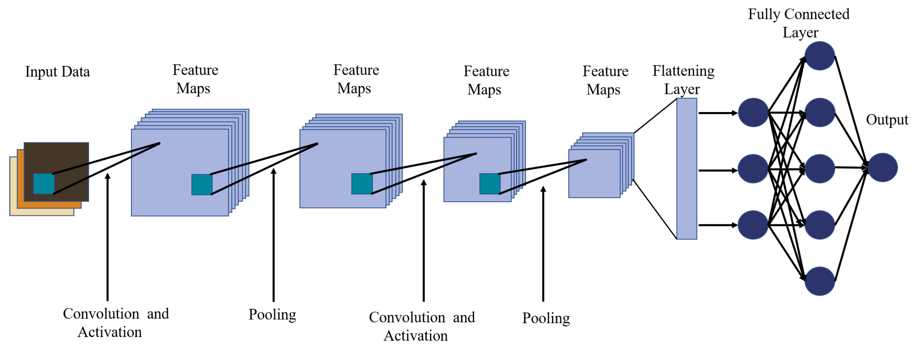This helps avoid predictive biases found in conventional approaches and ensures accurate forecasts in complex data settings [14]. To tackle the prevalent issues of multimodal data processing in vegetation productivity prediction, we suggest integrating TTHHO with a regression model with parallel computing capabilities and efficient optimization, namely CNN-LSSVM. Utilizing CNN to process spatially correlated data, LSSVM can proficiently execute regression analysis based on features derived from various data sources, markedly improving the multi-factor predictive performance.

Conventional point prediction techniques frequently neglect the uncertainty inherent in forecasts, particularly when addressing extremely dynamic data [15]. A solitary prediction of vegetation cover frequently inadequately represents the actual data conditions [16]. Using confidence intervals for interval probability prediction helps to clearly show the uncertainty in the predicted outcomes. 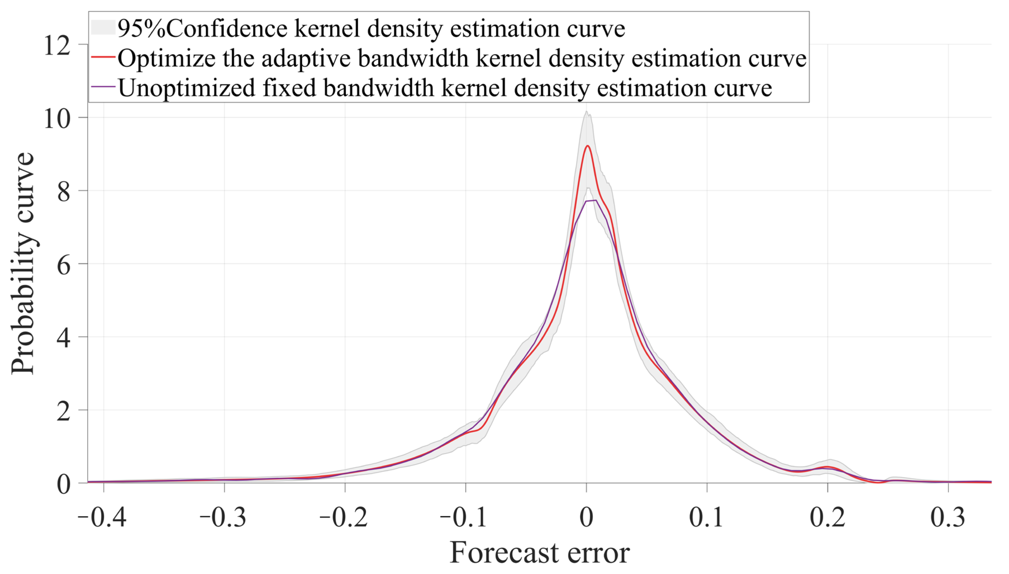In contrast to conventional point prediction, interval probability prediction offers not only the expected value but also its confidence interval, which signifies the likelihood of the prediction residing within a designated range, thus more thoroughly representing the potential variability of the data [17]. Adaptive Bandwidth Kernel Density Estimation (ABKDE) offers a novel method for evaluating the probability density function of prediction errors, facilitating the accurate identification of data instability [18]. When the data include outliers, interval prediction can accommodate data variability, offering an expanded range for the predicted value and diminishing dependence on a singular value, thereby improving the model’s resilience and stability [19]. Recent studies show that integrating ABKDE with machine learning models helps to improve distribution estimates. This approach better handles outliers and noise, reduces data interference, and enhances model resilience [20]. In multi-factor prediction tasks for vegetation productivity, ABKDE-based interval prediction uses probability density estimates to represent the data’s variance and uncertainty. While ABKDE shows promise in predicting multi-factor interval probabilities for vegetation productivity, further optimization is needed to address issues with high-dimensional data and outlier prediction.

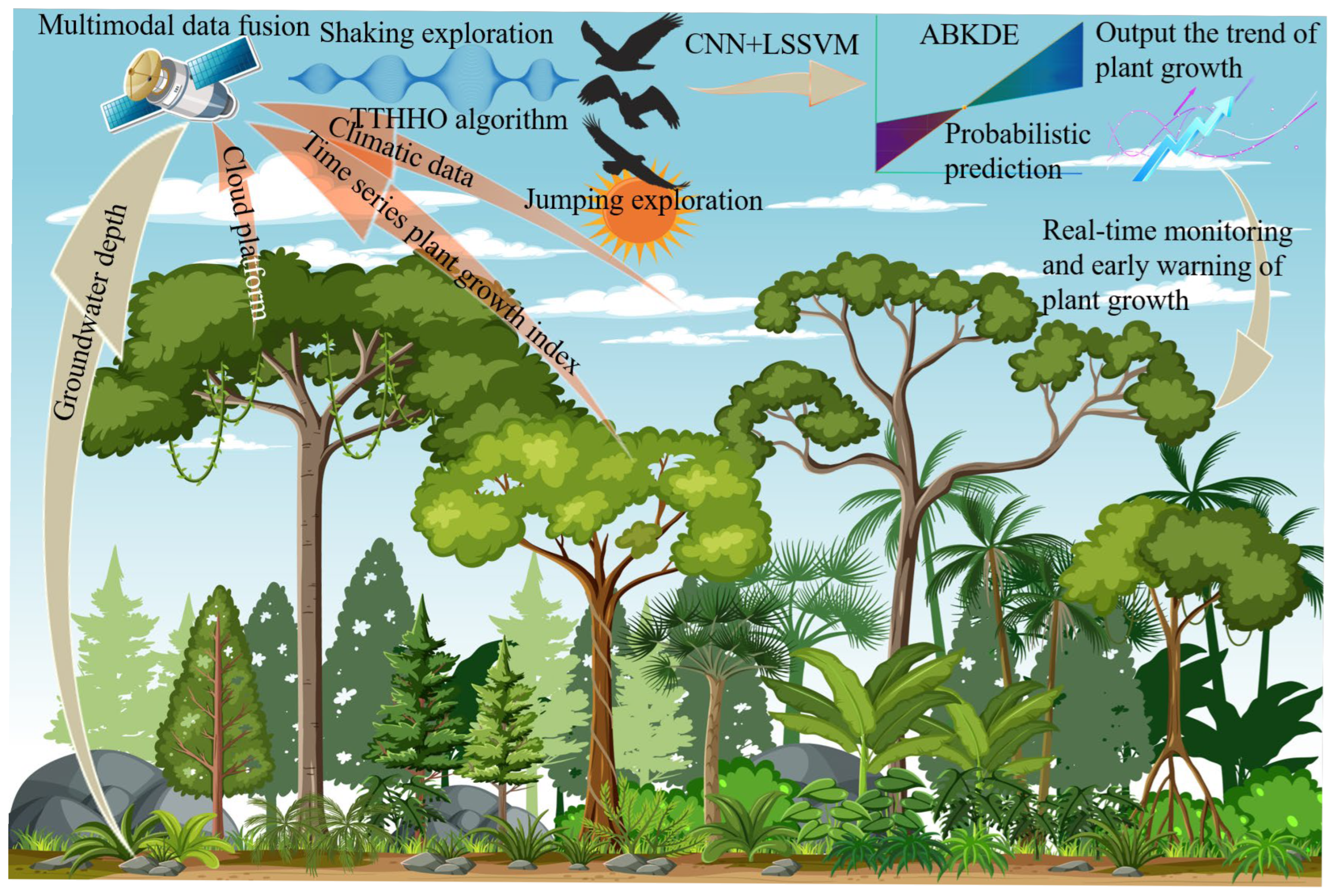
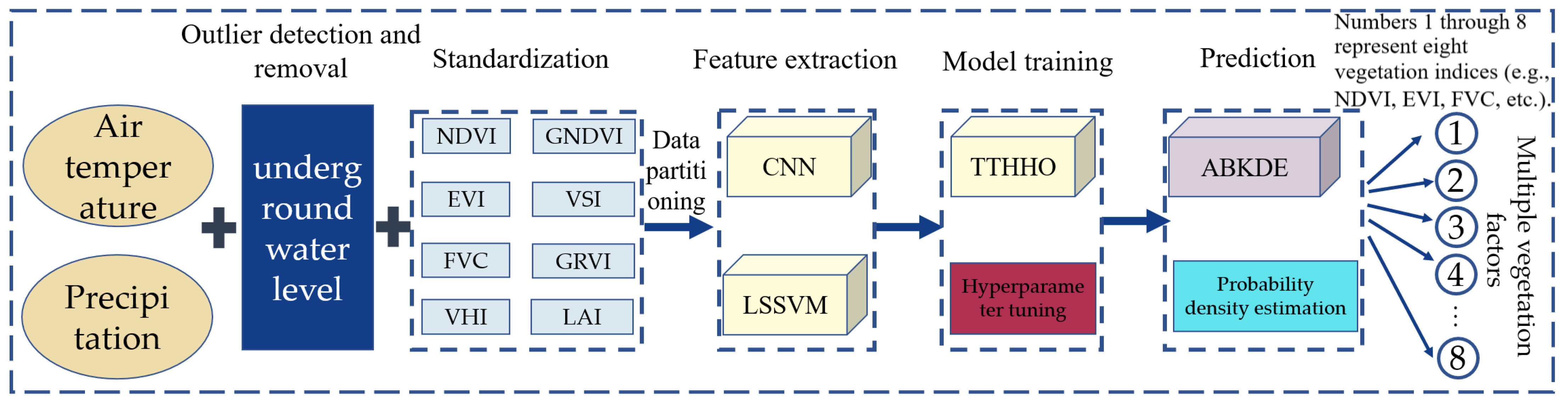
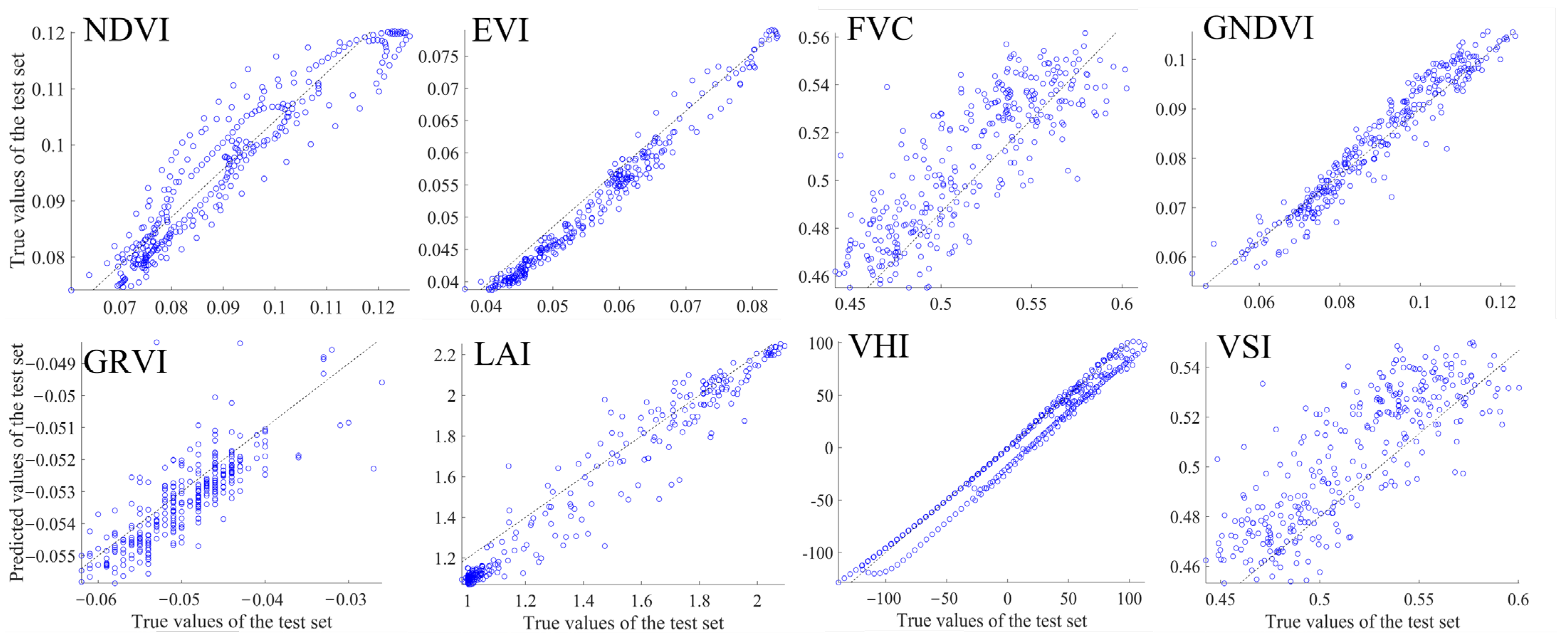
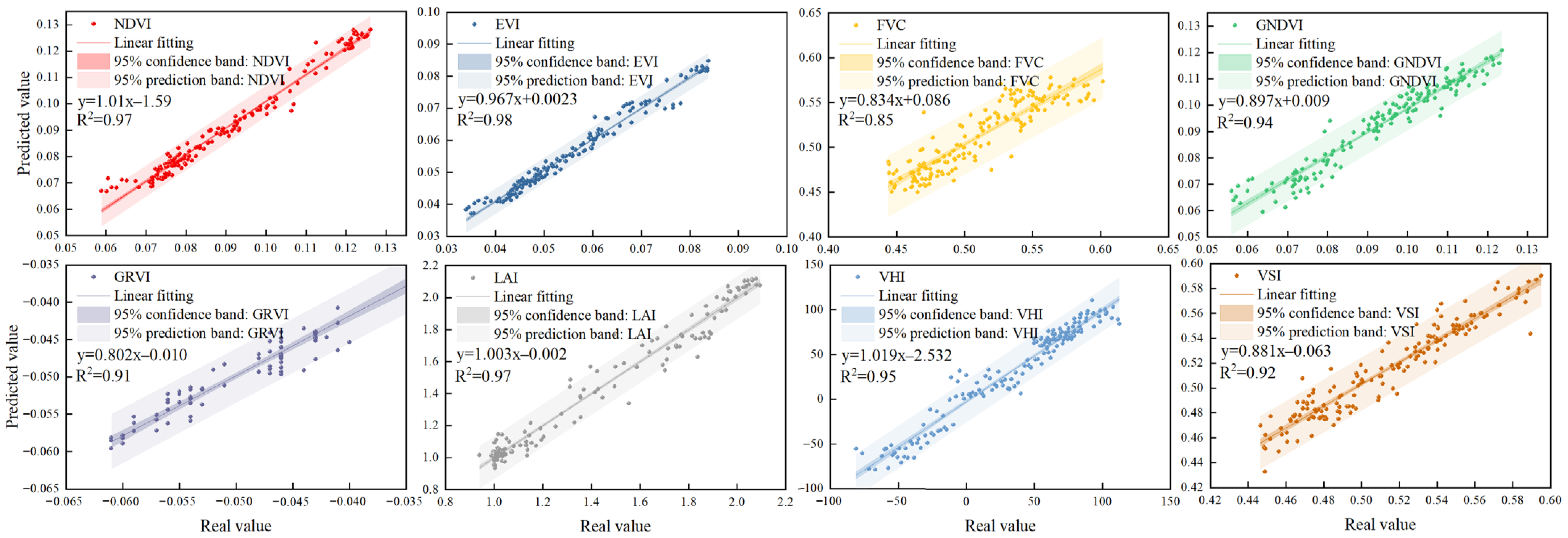
This paper introduces the TCLA technique, which integrates the TTHHO algorithm, CNN-LSSVM, and ABKDE model, to address two fundamental issues in conventional machine learning: the accuracy of regional probability predictions and resilience against interference. We chose the Hetao Irrigation District, China’s most significant irrigation region, as the research site to assess the model’s efficacy. The TTHHO algorithm navigates the search space and optimizes network node placements using multimodal data, including climate data, groundwater levels, and vegetation indices. The model’s robustness is improved by integrating CNN-LSSVM for feature extraction and regression analysis. ABKDE is also introduced to estimate the probability density function and identify outliers. This technique effectively performs region-specific probability prediction for several vegetation productivity parameters (NDVI (Normalized Difference Vegetation Index), EVI (Enhanced Vegetation Index), FVC (Fractional Vegetation Cover), VHI (Vegetation Health Index), GNDVI (Green Normalized Difference Vegetation Index), VSI (Vegetation Stress Index), GRVI (Green-Red Vegetation Index), and LAI (Leaf Area Index)) and demonstrates considerable resilience to interference. The principal advances of this work are as follows:

(1)

TTHHO intelligently explores the search space and adaptively optimizes network node placements, improving the model’s capacity to manage multimodal data. Compared to conventional approaches, TTHHO can more precisely analyze multi-factor data and enhance the network architecture, substantially increasing the accuracy of vegetation productivity forecasts. This study uses TTHHO as outlined in Section 2.4.2, differing from Abdulrab H’s original proposal of the TTHHO algorithm [12], which primarily assessed the algorithm’s advantages relative to conventional approaches. We present the inaugural application of TTHHO to a machine learning model, incorporating targeted enhancements and optimizations to its hyperparameters. It has been effectively utilized in the development of a practical model to improve the accuracy of vegetation productivity forecasts.

(2)

This research presents ABKDE for estimating probability density functions and detecting outliers. This invention successfully mitigates prediction bias in conventional models when encountering outliers. This study uses ABKDE as outlined in Section 2.5.3. In contrast to Liu et al.’s CBGRU-ABKDE-WT model [20], we innovatively incorporate the bootstrap method to generate prediction intervals, providing upper and lower bounds for forecasts and thereby enhancing the model’s credibility.

(3)

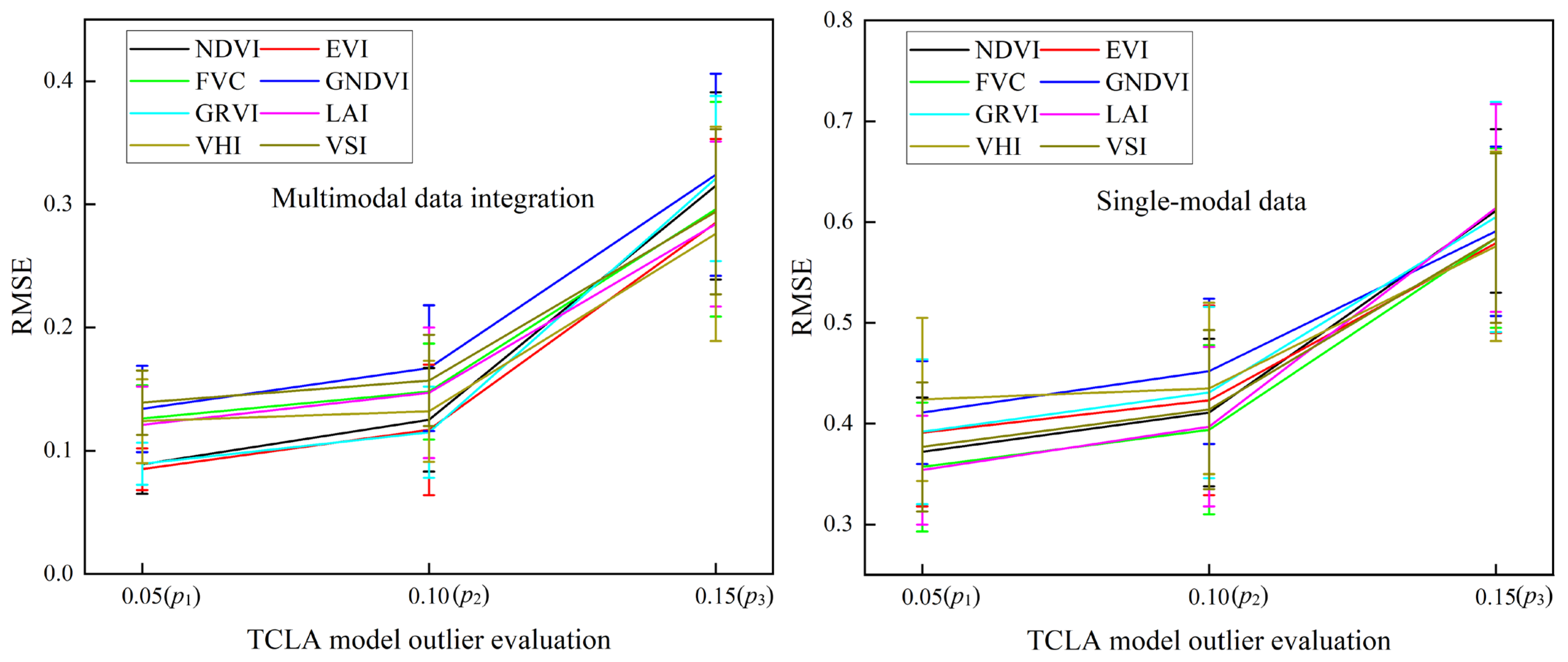
This research effectively combines TTHHO, CNN-LSSVM, and ABKDE to provide multi-factor regional probability forecasting for vegetation productivity. The model exhibits enhanced resilience to interference, considerably improving its robustness and precision in real applications, particularly when confronted with 5–15% outliers.

2. Materials and Methods

2.1. Study Area

This study picks the Hetao Irrigation District, the largest irrigation area in China’s designated irrigation region, to assess the efficacy of the multimodal model. The present irrigated area is 5560 km², and the study area’s location and particular monitoring sites are depicted in Figure 1 [21]. The study area is characterized by a temperate, arid, and semiarid continental climate, with cold winters with minimal snowfall, hot and arid summers, significant diurnal temperature fluctuations, extended hours of sunlight, and concurrent availability of light, heat, and water. The frost-free duration is around 130 days, conducive to vegetative development. The mean annual precipitation is 148.8 mm, whereas the mean annual evaporation is 2327 mm. In the growth season (May to September), precipitation constitutes about 85% of the yearly rainfall [22]. Recent advancements in irrigation technology and stronger ecological protection measures have increased plant cover in the irrigation district. These improvements have also enhanced the stability of agricultural production. In certain regions, excessive reclamation and imprudent water resource management have led to vegetation deterioration and land desertification. Climate dryness and anthropogenic activity have resulted in significant vegetation degradation in some regions, complicating ecological restoration efforts and presenting potential threats. Vegetation productivity, a vital indication of vegetation production, is essential for correctly evaluating the vegetation’s growth condition and carbon sink potential in the Hetao Irrigation District. Consequently, there is an imperative want for a methodology that can accurately forecast vegetation resources, systematically manage vegetation productivity, and furnish efficient decision-making assistance for ecological conservation and resource management.

2.2. Data and Processing

2.2.1. Remote Sensing Data Source

This study calculated vegetation productivity using the Google Earth Engine (GEE) cloud platform (1 January 2025). It extracted several vegetation indices to assess the growth state of vegetation. The multi-source remote sensing data originated from the Landsat and MODIS satellite series. Utilizing the robust data processing capabilities of the GEE platform, we preprocessed data from various sources, standardized it, and removed extraneous interferences, such as clouds and shadows, to guarantee data quality and consistency [23]. We identified eight remote sensing indices exhibiting a robust linear correlation with vegetation productivity: NDVI, EVI, FVC, VHI, GNDVI, VSI, GRVI, and LAI, with comprehensive calculations presented in

Table 1. Calculation of vegetation index.

Vegetation Index	Computational Formula	Formula Symbol Interpretation	References
NDVI	$NDVI={\displaystyle \frac{NIR-RED}{NIR+RED}}$	NIR indicates the reflectance of the near-infrared band, and RED indicates the reflectance of the red band.	[24]
EVI	$EVI=G\cdot {\displaystyle \frac{NIR-RED}{NIR+C_1 \cdot RED-C_2 \cdot BLUE+L }}$	G is the gain factor, C1, C2, and L are constants, and BLUE is the reflectance of the blue band.	[25]
FVC	$FVC={\displaystyle \frac{NDVI-NDV{I}_{min}}{NDV{I}_{max} -NDV{I}_{min}}}$	NDVImin and NDVImax are the minimum and maximum NDVI values.	[24]
VHI	$VHI={\displaystyle \frac{NDVI-VH{I}_{min}}{VH{I}_{max} -VH{I}_{min}}}$	VHImin and VHImax are the minimum and maximum VHI values.	[26]
GNDVI	$GNDVI={\displaystyle \frac{NIR-GREEN}{NIR+GREEN}}$	GREEN indicates the reflectance of the green light band.	[26]
VSI	$VSI= {\displaystyle \frac{NDVI-NDV{I}_{min}}{NDV{I}_{max} -NDV{I}_{min}}}$		[27]
GRVI	$GRVI={\displaystyle \frac{GREEN-RED}{GREEN+RED}}$		[28]
LAI	$LAI={\displaystyle \frac{NIR}{RED}}$		[29]

. We generated time-series data of several vegetation indices from 2011 to 2023. We included multimodal data (climate and groundwater levels) as input features to assess the accuracy and contribution of each vegetation indicator in predicting vegetation productivity.

2.2.2. Groundwater Depth Data Monitoring

This study utilized groundwater depth data obtained from specialized monitoring wells at the Dengkou experimental site, including a well depth of 80 m, mainly focusing on restricted water and pore water layers. The monitoring system uses an automated water level recorder to collect groundwater data daily. The data are sent, in real time, to a cloud-based database for storage. Data collection follows established hydrological monitoring standards. Raw water-level data are calibrated and validated against reference sites to ensure consistency over time and across locations. The monitoring equipment acquires water-level variation data using pressure sensors (Beijing Sinton Technology Co., Ltd., Beijing, China), exhibiting a precision of ±0.5 mm. The statistical metrics for the groundwater depth data are as follows: mean of 10.69 m, maximum of 12.3 m, minimum of 9.4 m, standard deviation of 0.96 m, coefficient of variation of 0.09, skewness of −0.45, and kurtosis of −1.66. The data-collecting period extends from January 2011 to December 2023, with a daily time step encompassing 14 monitoring sites.

2.2.3. Climatic Data Sources

The primary meteorological data for this study were sourced from the fifth-generation ECMWF Atmospheric Reanalysis Global Data Set (ERA5) provided by the GEE cloud platform [30]. This dataset covers the period from 2000 to 2023, with a spatial resolution of 0.1° × 0.1°, and includes daily temperature and precipitation data, specifically the following:

• Precipitation data are sourced from the ECMWF/ERA5_LAND/DAILY_AGGR dataset, specifically the total_precipitation_sum.
• Temperature data are selected from the same dataset, using temperature_2 m, representing daily average values calculated from hourly temperature observations 2 m above the ground.

Daily precipitation is obtained through cumulative calculations during data preprocessing, while time-weighted averages of hourly observations generate temperature data. This results in a spatiotemporal continuous sequence of meteorological input variables, the statistical indicators of climate data are shown in

Table 2. Statistical indicators of climate data.

Climatic Data	Time Range	Mean	Maximum	Minimum	Standard Deviation	Coefficient of Variation
Precipitation	2011.1–2023.12	0.00037	0.032 m	0 m	0.0019	5.04
Temperature	2011.1–2023.12	10.27	33.44 °C	−21.05 °C	12.75	1.24

.

2.3. Framework for TCLA Methods

Vegetation productivity is an essential component of ecosystems, primarily influenced by various factors, such as the climate, soil, vegetation, and groundwater. This study uses CLA as the base network. It combines it with the Transient Trigonometric Harris Hawks Optimizer to construct the TCLA model, incorporating groundwater levels and climate data as auxiliary variables to accurately capture the impact of multiple factors on vegetation productivity (as seen in Figure 2). The TCLA model consists of four main components—the TTHHO algorithm, CNN, LSSVM, and ABKDE modules. The overall process is shown in Figure 3, and the contribution of each component is detailed in

Table 3. The contribution of each component of the TCLA model.

Component	Role	Contribution
TTHHO	Optimization algorithm	Optimizes the hyperparameters (gamma, sigma) of LSSVM by balancing exploration and exploitation in the search space.
CNN	Feature extraction	Extracts relevant features from raw data, particularly in spatial or temporal contexts, enabling better input for LSSVM.
LSSVM	Prediction model	Performs regression or classification based on the features extracted by CNN and the optimized hyperparameters from TTHHO.
ABKDE	Density estimation and outlier detection	Provides probability density estimation and helps detect and handle outliers, improving the robustness and accuracy of predictions.

. TTHHO performs well with long time series of vegetation productivity. It can dynamically adjust both global and local search behavior, avoiding premature convergence to local optima. This ensures that the most relevant variables are included in the CLA model. By integrating it with the CLA model, CNN and LSSVM can map the input data to a high-dimensional space using kernel functions, thereby capturing complex nonlinear relationships. ABKDE improves the estimation process by using the adaptive bandwidth. It adjusts according to the data density in different vegetation productivity regions, enhancing the performance of vegetation productivity time-series prediction. The proposed method has three main innovations: (1) the transient trigonometric function of TTHHO will be employed to dynamically adjust the balance between exploration and exploitation, with the goal of efficiently finding the optimal parameter combination within the solution space. (2) The TCLA model is designed to address the nonlinear relationships among multi-source information, such as groundwater levels, climate data, and remote sensing data, in order to optimize the accuracy of vegetation productivity prediction through spatial estimation capabilities. (3) The TCLA model is designed to adapt to complex environments in arid and cold regions, with the objective of improving prediction accuracy by identifying suitable parameter combinations. This is particularly aimed at areas where there is significant spatial heterogeneity in vegetation productivity. In order to achieve high accuracy while reducing the computational cost, we referenced previous studies and specifically optimized the TCLA model [12,14,19,20]. The corresponding hyperparameter settings are shown in

Table 4. Model parameter settings.

Parameter	Value
Population size	300
Maximum iterations	150
Lower bound	[10, 0.1]
Upper bound	[1000, 100]
Dim	2
Type	F (regression)
Kernel	RBF(Radial Basis Function)_kernel
Proprecess	Preprocess
Gamma	Best_Pos (1)
Sigma	Best_Pos (2)
Z	[0.975; 0.95; 0.875; 0.75; 0.625; 0.55; 0.525]
Eta	0.5
Time_index	[25; 50; 75; 200]
Num_KD	Numel (time_index)
Convolution_kernel_size	[1, 5]
Filters	16
Activation function	ReLU
MaxPooling layer	2 × 2, stride = 7
Normalization	BatchNormalization Layer
Fully connected layer	32
Optimizer	Adam
Kernel function	Radial Basis Function (RBF) kernel
C (regularization parameter)	>0
Gamma	[0, 100]
Sig2	[0, 1]

.

2.4. Transient Trigonometric Harris Hawks Optimizer

TTHHO is an enhanced hybrid optimization method derived from the conventional Harris Hawks Optimizer. This algorithm’s benefit is its capacity to intelligently navigate the search space and adaptively optimize grid node positions [8]. It amalgamates the advantages of HHO (Harris Hawks Optimizer), SCA (Sine Cosine Algorithm), and TSO (Tuned Search Optimization). TTHHO can dynamically adjust the transition between exploration and exploitation using transient trigonometric functions. This allows the model to achieve a better balance between global search and local optimization [10]. Due to the complexity and variability of vegetation productivity time-series data, which is marked by significant geographical differences, TTHHO can make frequent large leaps within the search region. This enhances the effectiveness of vegetation productivity prediction. Furthermore, TTHHO, based on the adaptive modification of the search method, may more effectively identify the ideal parameter combination for the LSSVM and ABKDE models.

2.4.1. Transient Search Optimizer

The TSO algorithm is based on circuit system dynamics. It is derived from the mathematical modeling of the oscillatory properties of a second-order RLC circuit and the decay dynamics of a first-order discharge circuit [31]. This technique combines global search with local optimization by mimicking the transient response in the circuit system. Its global exploration approach is informed explicitly by the oscillation mode of the RLC resonant circuit at critical damping. In contrast, the local exploitation mechanism is derived from the exponential decay properties of voltage in a resistor–capacitor (RC) circuit (as seen in Figure 4) [8]. TSO incorporates a random variable (r₇) to ascertain the inclination towards exploration or exploitation. Furthermore, the circuit’s steady-state solution x(∞) is obtained from the optimum solution y_best. The precise mathematical model is delineated as follows:

$$y(t)=y(\infty )+(y(0)-y(\infty ))e^{-t/\tau }$$

(1)

where t represents time, y(t) corresponds to the capacitor voltage v(t) in an RC circuit or the inductor current i(t) in an RL circuit, and τ is the time constant of the circuit, which is equal to the product of the resistance R and the capacitance C in the RC circuit [32].

$$y(t)=e^{-\alpha t}\left(B_1\cos (2\pi f_{d}t)+B_2\sin (2\pi f_{d}t)\right)+y(\infty )$$

(2)

where α is the damping coefficient, f_d is the damping resonant frequency, and B₁ and B₂ are constants.

$$y_{t+1}=\left\{\begin{array}{ll}{y}_{best}+(y_t-C_1\cdot y_{best})e^{-L},\hfill & r_7<0.5\hfill \\ y_{best}+e^{-L}\left[\cos (2\pi L)+\sin (2\pi L)\right]\cdot |y_t-C_1\cdot y_{best}|,\hfill & r_7\ge 0.5\hfill \end{array}\right.$$

(3)

2.4.2. Improvements to the Transient Trigonometric Harris Hawks Optimizer

This paper presents a three-layer collaborative optimization system employing a hierarchical progressive multi-strategy integration mechanism. This design decomposes the optimization work into three tiers: the top tier, middle tier, and bottom tier, which are cooperatively implemented by the HHO, SCA, and TSO, as seen in Figure 5 [9]. The highest level configures M HHO search agents, each corresponding to M SCA populations at the intermediate level, with each SCA population including N optimization individuals. The optimization process begins at the lower and intermediate levels. TSO is responsible for iteratively refining candidate solutions generated by SCA. At the same time, SCA optimizes and modifies the original solutions supplied by HHO [11]. Each tier identifies the optimal solution using a fitness evaluation mechanism during the iterative process. Information is transmitted through the hierarchical structure, as shown in Figure 6. The premier HHO adjusts its locations according to the supplied optimization data, attaining a dynamic equilibrium between global exploration and local exploitation, to integrate the advantages of HHO, SCA, and TSO, thereby improving convergence and the quality of the solution. See

Table 5. Comparison of algorithm characteristics and application scenarios.

Algorithm	Exploration Capability	Exploitation Capability	Algorithm Complexity	Convergence Speed	Parameter Tuning Difficulty	Suitable Application Scenarios
TTHHO	Strong (jumping + oscillation)	Strong (fine-grained search)	High	Fast	High	Complex constraints, multi-objective optimization problems
HHO	Moderate (group collaboration)	Relatively strong	Medium	Moderate	Medium	Scenarios emphasizing local optimization accuracy
SCA	Strong (broad oscillation)	Moderate	Low	Average	Low	Suitable for rapid search, preliminary global exploration
TSO	Relatively strong (global jumps)	Weak	Low	Average	Low	Primarily global exploration, rapid initial optimization

. This hierarchical cooperation mechanism, via multi-scale information interaction, successfully prevents premature convergence and improves the algorithm’s optimization accuracy and convergence time.

The following equation represents the TTHHO exploration phase model, where the energy of prey escape satisfies |E| ≥ 1, and its energy is derived from the hunting behavior of the Harris hawk [8]. The behavioral characteristics of the bottom and middle layers are represented by the symbols A, B, C, and D, where t denotes the current iteration number, and T is the maximum number of iterations.

$$y_{t+1}=\left\{\begin{array}{ll}{y}_{rand}-r_1\ast |y_{rand}-2\ast r_2\ast [A]|,\hfill & r_3<0.5,r_7<0.5 \mathrm{and} q<0.5\hfill \\ y_{rand}-r_1\ast |y_{rand}-2\ast r_2\ast [B]|,\hfill & r_3<0.5,r_7\ge 0.5 \mathrm{and} q<0.5\hfill \\ y_{rand}-r_1\ast |y_{rand}-2\ast r_2\ast [C]|,\hfill & r_3\ge 0.5,r_7<0.5 \mathrm{and} q<0.5\hfill \\ y_{rand}-r_1\ast |y_{rand}-2\ast r_2\ast [D]|,\hfill & r_3\ge 0.5,r_7\ge 0.5 \mathrm{and} q<0.5\hfill \\ [y_{best}-Y_m]-r_1\ast (r_2(u_b-l_b)+l_b),\hfill & q\ge 0.5\hfill \end{array}\right.$$

(4)

$$\begin{array}{l}A=y_{best}+(y_t-C_1\ast y_{best})e^{-L}+r_1\sin (r_5)\times |r_6\ast y_{best}-(y_{best}+(y_t-C_1\ast y_{best})e^{-L})|\\ B=y_{best}+e^{-L}\left[\cos (2\pi L)+\sin (2\pi L)\right]|y_t-C_1\ast y_{best}|+r_1\sin (r_5)\times |r_6\ast y_{best}-\\ (y_{best}+e^{-L}\left[\cos (2\pi L)+\sin (2\pi L)\right]|y_t-C_1\ast y_{best}|)|\\ C=y_{best}+(y_t-C_1\ast y_{best})e^{-L}+r_1\cos (r_5)\times |r_6\ast y_{best}-(y_{best}+(y_t-C_1\ast y_{best})e^{-L})|\\ D=y_{best}+e^{-L}\left[\tan (2\pi L)+\sin (2\pi L)\right]|y_t-C_1\ast y_{best}|+r_1\cos (r_5)\times |r_6\ast y_{best}-\\ (y_{best}+e^{-L}\left[\tan (2\pi L)+\sin (2\pi L)\right]|y_t-C_1\ast y_{best}|)|\end{array}$$

(5)

$$\begin{array}{l}{E}_1=2\ast \left(1-{\displaystyle \frac{t}{T}}\right)\\ L=2\ast r_1\left(1-E_1\right)\\ C_1=K\ast r_2\ast E_1+1\\ E_0=2\ast r_1-1\\ E=E\ast E_0\\ r_5=2\pi \ast rand()\\ r_6=2\ast rand()\\ K=1\\ J=2(1-r_1)\end{array}$$

(6)

In the equation, r₁, r₂, r₃, r₄, r₇, and q are stochastic parameters uniformly distributed within the interval [0, 1], where y_best denotes the current optimal transient solution, y_t signifies the current solution, Y_m represents the overall mean, u_b indicates the upper limit, and lb refers to the lower bound.

The HHO and its enhanced variant, TTHHO, are based on the mathematical modeling of Harris hawk hunting behavior. This is described by the predator–prey dynamic model [33]. The program emulates the hunting behaviors of predators across many settings, developing an optimization process that encompasses four distinct modes: (1) hard encirclement strategy; (2) hard encirclement with rapid approach strategy; (3) soft encirclement strategy; (4) soft encirclement with rapid approach strategy. The strategy selection process employs two criteria: prey escape energy E (E ∈ [0, 1]) and the random disturbance factor r (r ∈ [0, 1]) [34]. The subsequent formulae delineate the mathematical representations of these strategies:

$$y_{t+1}=\left\{\begin{array}{ll}{y}_{prey}-E\ast |y_{prey}-2\ast r_2\ast [A]|,\hfill & r_3<0.5\mathrm{and}{r}_7<0.5\hfill \\ y_{prey}-E\ast |y_{prey}-2\ast r_2\ast [B]|,\hfill & r_3<0.5\mathrm{and}{r}_7\ge 0.5\hfill \\ y_{prey}-E\ast |y_{prey}-2\ast r_2\ast [C]|,\hfill & r_3\ge 0.5\mathrm{and}{r}_7<0.5\hfill \\ y_{prey}-E\ast |y_{prey}-2\ast r_2\ast [D]|,\hfill & r_3\ge 0.5\mathrm{and}{r}_7\ge 0.5\hfill \end{array}\right.$$

(7)

where y_prey denotes the optimal position of the prey, whereas y_best signifies the temporary best answer. When the stochastic disturbance parameter r is less than 0.5, the algorithm transitions into a high-intensity exploitation phase, employing a hybrid approach that integrates hard encircling with increasing rapid dives [9]. In this mode, the algorithm’s search approach exhibits distinct spatial contraction traits: global exploration diminishes progressively, whilst local exploitation capabilities are markedly intensified. This strategic shift allows search agents to identify and secure potential optimal solutions with higher fitness values. This improves the algorithm’s convergence rate [8]. The algorithm’s search procedure during this phase may be articulated using the subsequent mathematical model:

$$Y_{t+1}^i=\left\{\begin{array}{l}Z ifF(Z)<F(y_t)\&\hfill \\ y_t=\left\{\begin{array}{l}A,\hspace{1em}{r}_3<0.5\mathrm{and}{r}_7<0.5\hfill \\ B,\hspace{1em}{r}_3<0.5\mathrm{and}{r}_7\ge 0.5\hfill \\ C,\hspace{1em}{r}_3\ge 0.5\mathrm{and}{r}_7<0.5\hfill \\ D,\hspace{1em}{r}_3\ge 0.5\mathrm{and}{r}_7\ge 0.5\hfill \end{array}\right.\hfill \\ X ifF(X)<F(y_t)\&\hfill \\ y_t=\left\{\begin{array}{l}A,\hspace{1em}{r}_3<0.5\mathrm{and}{r}_7<0.5\hfill \\ B,\hspace{1em}{r}_3<0.5\mathrm{and}{r}_7\ge 0.5\hfill \\ C,\hspace{1em}{r}_3\ge 0.5\mathrm{and}{r}_7<0.5\hfill \\ D,\hspace{1em}{r}_3\ge 0.5\mathrm{and}{r}_7<0.5\hfill \end{array}\right.\hfill \end{array}\right.$$

(8)

where u and v are random variables ranging from 0 to 1, and σ represents the constant value 1.5. This work employs the TTHHO method to optimize the hyperparameters of the LSSVM model, namely gamma and sigma, which regulate the model’s complexity and the kernel’s width, both of which are essential for the model’s performance. The precise hyperparameter configurations are as follows: N = 300 is selected to balance the diversity of solutions with computational expense; MaxIt = 100 is established based on the problem’s complexity and empirical findings, which is adequate for the algorithm to converge to an optimal solution; LB = [10, 0.1] and UB = [1000, 100] delineate the search boundaries for gamma and sigma, established according to empirical values of LSSVM to ensure that TTHHO operates within a practical range; dim = 2 signifies that two hyperparameters (gamma and sigma) require optimization. The tuning process of TTHHO employs a combination of exploration and exploitation strategies. Initially, the algorithm broadly explores the solution space to identify potential optimal solutions, but in subsequent phases, it focuses on refining the existing best solution. All hyperparameters are optimized using cross-validation and grid search techniques to ensure the model’s optimal performance.

2.5. CLA Methods

Under intricate climatic situations like drought and cold, geographical data of vegetation productivity demonstrate considerable variation and robust association. The input variables for vegetation productivity prediction, such as remote sensing data, climatic indicators, and groundwater levels, generally exhibit high dimensionality and encompass intricate spatiotemporal interactions. Conventional deep learning models find it challenging to represent their nonlinear characteristics accurately. This work extracts multi-level features from various input data, such as groundwater levels, precipitation, and temperature. It uses the convolutional layers of CNN to improve the modeling efficiency of LSSVM. Concurrently, LSSVM employs kernel functions to transform the input data into high-dimensional space, elucidating intricate nonlinear connections. Consequently, ABKDE is used to assess the geographical distribution of LSSVM prediction outcomes, thereby enhancing the precision of the long-term time-series forecasts of regional vegetation productivity. This CLA model is an effective instrument for monitoring, managing, and predictive analysis of vegetation resources.

2.5.1. Convolutional Neural Network

With its distinctive hierarchical feature-extraction technique, CNN has shown considerable benefits in image processing, time-series data modeling, and feature learning [19]. The design primarily comprises convolutional, pooling, and fully linked layers, allowing the adaptive processing of heterogeneous input via multi-scale feature extraction, as seen in Figure 7. Unlike conventional feature engineering techniques, CNN uses learnable convolutional kernels (W) and automatically extracts high-order features from the data through a sliding window mechanism. This reduces the complexity of manual feature construction [35]. When combined with ABKDE, the model fully utilizes the spatial feature information gathered by CNN. This improves the accuracy of local density estimates in vegetation productivity time-series prediction, enhancing the precision of spatial distribution patterns. The computational procedure is as follows:

$$p\prime ={\displaystyle \frac{2\left(p-p_{\min }\right)}{p_{\max }-p_{\min }}}-1$$

(9)

where p is the input feature value, and p_min and p_max are the minimum and maximum values of the feature, respectively. Local temporal features are extracted through convolution operations, as shown in Equation (10):

$$h_{i,j}^{\left(k\right)}={\displaystyle \int \left({\displaystyle \sum _{\mathrm{m}=1}^M{\displaystyle \sum _{\mathrm{n}=1}^N{x}_{i+m,j+n}\bullet w_{m,n}^{\left(k\right)}+b^{\left(k\right)}}}\right)}$$

(10)

where x_{i, j} denotes the input picture’s pixel value, representing the convolutional kernel’s weight, b^(k) signifies the bias term, and ∫ indicates the activation function. The pooling layer is a key component of convolutional neural networks. It reduces the dimensionality of feature maps produced by the convolutional layer through down-sampling. This layer executes feature aggregation over local regions utilizing designated pooling functions, hence diminishing the spatial resolution of the feature map. This dimensionality reduction technique has two main benefits. It reduces the number of network parameters and computational complexity. At the same time, it improves the model’s resilience by preserving the most important features. The pooling layer ultimately produces the down-sampled feature representation, as indicated in Equation (11):

$$y_{i,j}=\max \left(x_{i+m,j+n}\right), \mathrm{m}, \mathrm{n}\in \{0, 1,\dots , k-1\}$$

(11)

where k is the pooling window size. Max pooling helps retain the most significant information from the convolutional features and reduces the size of the feature map.

2.5.2. Least Squares Support Vector Machine

LSSVM, an optimized variant of Support Vector Machine (SVM), reformulates the inequality constraints of conventional SVM into equality constraints, thus converting the quadratic programming solution of the original problem into the resolution of a linear system of equations, as illustrated in Figure 8 [36]. This method reduces the computational complexity and improves the algorithm’s operational efficiency [37]. In climate and forest vegetation index data characterized by noise interference and uncertain characteristics, LSSVM, integrating its linear regression framework with a least squares optimization technique, exhibits superior prediction performance and resilience. This paper presents a hybrid modeling system that seamlessly blends CNN with LSSVM. This fusion technique leverages the strengths of CNN in feature extraction and LSSVM in regression prediction, resulting in effective modeling and precise prediction of complicated nonlinear connections in multi-source data. The model formulates an optimum decision function inside a high-dimensional feature space, converting the nonlinear estimating challenge into a linear estimation issue, as seen in Equation (12):

$$f(x_i)=w^T\times x_i+b,\hspace{1em}i=1,2,\dots ,N$$

(12)

where x_i = (x_i,1, x_i,2,…, x_i,D) represents the input data, with D being the dimensionality of the input data, N being the total number of samples, f(x_i) being the output value of the function, b being the bias, and w^T being the regression coefficients [36]. The model was further optimized by transforming the regression problem into the constrained optimization problem shown in Equation (13).

$$\left\{\begin{array}{l}\min J(w,\xi )={\displaystyle \frac{1}{2}}\Vert w{\Vert }^2+{\displaystyle \frac{\gamma }{2}}{\displaystyle \sum _{i=1}^N{\xi }_i^2}\hfill \\ \mathrm{s}.\mathrm{t}.\hspace{1em}{y}_i=w^T\times \phi (x_i)+b+{\xi }_i,\hspace{1em}\gamma \ge 0\hfill \end{array}\right.$$

(13)

where γ is the penalty factor, ξ_i is the slack variable, and φ(x_i) is the mapping from the low-dimensional space to the high-dimensional feature space [19]. On this basis, Lagrange multipliers are introduced to construct the Lagrange function, as shown in Equation (14), thereby achieving a more profound optimization of the model.

$$J(w,b,{\xi }_i,{\alpha }_i)=J(w,{\xi }_i)-{\displaystyle \sum _{i=1}^N{\alpha }_i}\left[w^T\phi (x_i)+b+{\xi }_i-y_i\right]$$

(14)

where α_i is the Lagrange multiplier; by deriving the Lagrange multipliers α_i bias b slack variables ξ_i, and regression coefficients w, the final result is obtained in Equation (15).

$$\left\{\begin{array}{c}{\displaystyle \frac{\partial L}{\partial w}}=0\to w={\displaystyle \sum _{i=1}^N{\alpha }_i}\phi (x_i)\\ {\displaystyle \frac{\partial L}{\partial b}}=0\to {\displaystyle \sum _{i=1}^N{\alpha }_i}=0\\ {\displaystyle \frac{\partial L}{\partial {\xi }_i}}=0\to {\alpha }_i=\gamma {\xi }_i\\ {\displaystyle \frac{\partial L}{\partial {\alpha }_i}}=0\to w^T\phi (x_i)+b+{\xi }_i-y_i=0\end{array}\right.$$

(15)

The optimization problem is transformed into the linear system of equations shown in Equation (16).

$$\left[\begin{array}{cc}0& I^T\\ I& \Omega +{\gamma }^{-1}I\end{array}\right]\left[\begin{array}{c}b\\ \alpha \end{array}\right]=\left[\begin{array}{c}0\\ y\end{array}\right]$$

(16)

where Ω = K(x_i, x_j) = φ(x_i)^T φ(x_j), y = [y₁, y₂, …, y_N]^T, a = [a₁, a₂, …, a_N]^T, and I is the identity vector. Therefore, the final output of the LSSVM model is obtained, as shown in Equation (17).

$$f(x_i)={\displaystyle \sum _{i=1}^N{\alpha }_i}K(x,x_i)+b$$

(17)

2.5.3. Adaptive Bandwidth Kernel Density Estimation

KDE, as a non-parametric probability density estimation method, estimates the probability density function of a random variable by smoothing data points [37]. Suppose the prediction error sequence is er = [er₁, er₂, …, er_n]. The expression for the probability density estimation at the point er can be represented as follows:

$$f_h(er)={\displaystyle \frac{1}{N\times h}}{\displaystyle \sum _{t=1}^{N}K}\left({\displaystyle \frac{er-e{r}_i}{h}}\right)$$

(18)

where N is the sample size, h represents the bandwidth, and K(⋅) denotes the kernel function. Studies indicate that conventional KDE has considerable constraints when addressing non-uniformly distributed data [37]. Due to the geographic variability of real-world observational data, fixed bandwidth techniques can result in two forms of estimate errors: significant bias in sparse areas and excessive smoothing in crowded places, thereby elevating the estimation variance [15]. This study uses ABKDE to solve the technical bottleneck. It creates a dynamic mapping between the bandwidth parameter and local data density, enabling the precise modeling of non-uniformly distributed data. This significantly improves the accuracy and reliability of density estimation. The PDF derived from ABKDE can be expressed as follows:

$$\widehat{f_{h_i}}(er)={\displaystyle \frac{1}{N}}{\displaystyle \sum _{t=1}^N\frac{1}{h_i(er)}}K\left({\displaystyle \frac{er-e{r}_i}{h_t(er)}}\right)$$

(19)

where h_i(er) is the adaptive bandwidth associated with the i-th sample point er_i at the estimation point er. The selection of this bandwidth is contingent upon the local density data of the sample sites, aiming to utilize a narrower bandwidth in regions of high density and a broader bandwidth in areas of low density, thereby enhancing the estimate precision [15].

To determine the optimal bandwidth for each local position, a Local Error Function (LEF) C_i(er_k) is defined and used to optimize the bandwidth for each estimation point. The expression is given as follows:

$$C_1(e{r}_k)=\widehat{f_h}{(e{r}_k)}^2-2\widehat{f_h}(e{r}_k)f(e{r}_k)+{\displaystyle \frac{2}{\sqrt{2\pi h_i}}}f(e{r}_k)$$

(20)

where er_k is the target estimation point, and h_i is the adaptive bandwidth associated with the target estimation point related to the sample point er_k. The LEF includes terms related to probability density estimation and actual values, considering bias and variance. The estimate’s accuracy is measured by $\widehat{f_h}{(e{r}_k)}^2$ and $2\widehat{f_h}(e{r}_k)f(e{r}_k)$ representing bias; ${\displaystyle \frac{2}{\sqrt{2\pi h_i}}}f(e{r}_k)$ is associated with the smoothness of the estimate and controls the variance of the model. The LEF attains a dynamic equilibrium between estimating precision and smoothness by optimizing bias and variance components [38]. The golden section search technique minimizes the LEF, precisely determining the ideal bandwidth parameters for each local location. This adaptive bandwidth selection approach improves KDE’s flexibility and estimation precision [15]. The LEF quantifies local estimate errors and provides guidance for bandwidth optimization. This enables ABKDE to handle data with complex distribution characteristics, offering an efficient solution to density estimation challenges.

For a given quantile z, the corresponding quantile solution q(z) can be obtained based on $\widehat{F}\left(er\right)$ and PI, resulting in the upper and lower bounds of the interval. The expression is as follows:

$$q(z)={\widehat{F}}^{-1}(e_r)$$

(21)

$$L{b}_i={\widehat{y}}_i+q(1-z)$$

(22)

$$U{b}_i={\widehat{y}}_i+q(z)$$

(23)

where ${\widehat{F}}^{-1}(e_r)$ is the inverse of the cumulative distribution function, ${\widehat{y}}_i$ is the predicted response value, and Lb_i and Ub_i are the lower and upper bounds of the i-th sample PI.

2.6. Experiment

2.6.1. Can Multimodal Data Improve the Accuracy of TCLA in Predicting Vegetation Productivity?

This study aims to evaluate the impact of multimodal data fusion on the predictive accuracy in regionally non-stationary vegetation productivity. We integrate climate data, remote sensing data, and groundwater level data into a single input vector. Vegetation productivity data, derived from remote sensing images, serve as the target variable. We propose that enough multimodal training data, coupled with the optimization of CNN and LSSVM hyperparameters using the TTHHO method, together with the adjustment of ABKDE bandwidth parameters, can substantially enhance the accuracy of vegetation productivity predictions. Consequently, we evaluated the performance of models using a single data source versus those using multimodal data sources to forecast vegetation productivity across 14 locations. Therefore, we constructed Transformer, LSTM, and TCLA models using NDVI, EVI, FVC, VHI, GNDVI, VSI, GRVI, and LAI data from 1 January 2011 to 1 June 2020, for training, and then forecasted NDVI, EVI, FVC, VHI, GNDVI, VSI, GRVI, and LAI data from June 2020 to December 2023 to assess the accuracy. This study evaluates the improvement in the vegetation productivity forecast accuracy using TCLA by comparing several models utilizing multimodal data.

2.6.2. The Necessity of Multimodal Data for Improving TCLA Model Prediction

The TCLA coupling approach that we present seeks to enhance the accuracy of vegetation productivity predictions. Multimodal data equip the model with multidimensional information, improving its comprehension of the variability patterns in vegetation productivity. The TTHHO method balances global exploration and local exploitation. It investigates potential correlations among data while managing multimodal datasets and enhancing model effectiveness through local optimization. Vegetation productivity is influenced by factors like climate, groundwater, and remote sensing data. A single optimization technique cannot adequately capture their complex interrelationships. TTHHO offers strong global search capabilities, while LSSVM efficiently handles large datasets and complex nonlinear relationships through kernel functions. ABKDE integrates multi-source information with adaptive bandwidth to build more accurate spatial and probability density models. The TCLA coupling model integrates various methodologies to enhance performance by utilizing multimodal data. This link augments the TCLA model’s expressiveness and resilience in managing intricate, multi-source data, improving the prediction accuracy by eliminating or attenuating noise. Provided the regional division remains constant, we developed four zoning methodologies: LSTM, Transformer, univariate TCLA, and multimodal data input TCLA. By comparing the models’ computational efficiency and accuracy, we substantiate the importance of multimodal data in enhancing TCLA model predictions.

3. Results

3.1. Comparison of Prediction Performance Across Various Algorithm Models

In the multi-factor prediction challenge concerning vegetation productivity, we evaluated the efficacy of standard models against the TCLA model. The results show that TCLA outperforms the LSTM and Transformer models in prediction accuracy and stability, especially in non-stationary and steady-state time-series data. In particular, the LSTM model exhibited poor predictive performance, achieving acceptable accuracy only for relatively stationary indices such as EVC and VHI, while failing to capture the nonlinear dependencies present in the other six vegetation indices (Figure 9). The model attained an R² value of 0.68 and an MAPE of 23.24% (

Table 6. Performance comparison of different models: LSTM, Transformer, TCLA (p < 0.01).

Model	R2	RMSE	MAPE (%)	Learning Rate	Batch Size	Training (s/Epoch)
LSTM	0.68a	0.95a	23.24a	0.001	128	0.69a
Transformer	0.75b	0.73a	14.32b	0.001	128	0.95a
TCLA	0.88c	0.41b	4.42c	0.001	128	5.94b

). This outcome indicates that LSTM exhibits limited predictive capacity for non-stationary data. In contrast, the Transformer model showed better trend-capturing ability in most vegetation factor predictions compared to the single-modality TCLA model. Nonetheless, the forecasts for GRVI, VHI, and LAI exhibited substantial fluctuations and failed to accurately capture the rapid variations in these variables (see Figure 10). The R² value was at 0.75, signifying that the Transformer model continues to encounter difficulties in managing intricate fluctuations.

The TCLA model showed a 12.66–23.61% improvement (p < 0.01) in prediction accuracy compared to conventional models (LSTM, Transformer) and produced results that were closer to the actual values. In repeated studies, we observed that TCLA’s convergence time was comparatively sluggish, indicating that its computing efficiency is inferior to that of traditional models (refer to Figure 11). Consequently, model selection must include computational efficiency and resource allocation. The model comparison experiment demonstrated that TCLA surpassed standard models in parameter optimization. The hierarchical structure facilitates a more comprehensive search for superior solutions throughout a more expansive parameter space. Conversely, conventional models, dependent on a singular optimization technique, exhibit constrained performance in intricate optimization challenges. This signifies that TCLA possesses superior tuning capabilities and optimization potential in intricate data contexts.

3.2. Multimodal Data Prediction Performance Evaluation

Predicting vegetation productivity requires evaluating multiple criteria. Models often need strong feature selection and dimensionality reduction to reduce the negative impact of redundant information on performance. To investigate the link between multimodal data, we performed a correlation study utilizing a chord diagram. The findings showed that temperature and precipitation have complex interactions with vegetation indices, while groundwater depth has stronger associations with various vegetation indices (see Figure 12). This suggests that both climate and groundwater depth may affect plant development. Based on this, this study consolidates varied information via multimodal data input. It examines its impact on the performance of the TCLA model, employing multiple confidence intervals and optimized ABKDE to assess prediction errors. For a comprehensive study, we amplified the vegetation characteristics by a factor of 100 for comparison.

The experimental findings indicate that the TCLA model, utilizing multimodal data input, markedly surpasses single-modality data input in predicting vegetation factors, achieving an overall accuracy enhancement of 3.57 ± 2.13%. The anticipated values of the TCLA model demonstrate exceptional predictive efficacy, with the prediction curve precisely reflecting the trend of the actual values (refer to Figure 13). The discrepancy between predicted and actual values is minimal at most sample sites, signifying that the model possesses robust trend-capturing skills. Incorporating multimodal data input leads to a substantial convergence of the confidence intervals in the TCLA model, resulting in less prediction uncertainty and affirming the model’s stability for future forecasts. At sampling point 25, the kernel density curve has a unimodal distribution, signifying a substantial concentration of model predictions at this location (refer to Figure 14). At sampling points 50, 75, and 200, the actual values predominantly reside in the kernel density curve’s high probability area, reinforcing the strong correspondence between model predictions and actual observations. Nonetheless, at specific sample sites, the exact values diverge from the apex of the kernel density curve, signifying that the model retains certain predictive inaccuracies.

A trend analysis indicates minimal discrepancy between projected and actual values (Figure 15a). The model has exceptional trend-capturing capability in stable areas of the data. A residual analysis indicates oscillations between expected and actual values; nevertheless, no consistent bias is seen (see Figure 15b). The residual distribution approximates a normal distribution, with the apex centered at 0, signifying that the model’s prediction error is minimal and uniformly distributed (refer to Figure 15c). The mean residual is 0.04, and the standard deviation is 0.081959, further corroborating the precision and consistency of the model’s predictions. The error distribution’s general form indicates that, regardless of whether using confidence intervals, optimized adaptive bandwidth kernel density curves, or fixed bandwidth kernel density curves, the errors are predominantly centered around 0, suggesting that the model has accurate predictive capability in most instances (see Figure 16). The optimized adaptive bandwidth kernel density estimation curve offers better prediction accuracy and fewer error fluctuations compared to the fixed bandwidth estimation. This indicates that the TCLA model, via bandwidth optimization, more adeptly captures the characteristics of error distribution, thereby markedly improving prediction reliability in multimodal data processing.

Upon examining the evaluation metrics of the TCLA model (PINAW, PICP, CRPS, CWC) across various confidence intervals (95%, 90%, 75%, 50%, 25%, 10%), it was determined that the TCLA model exhibits superior accuracy at diminished confidence intervals, particularly at the 10% CI, where the PINAW and PICP values are maximized, signifying that the model yields exact prediction intervals (refer to

Table 7. Model evaluation index and its confidence interval.

Evaluation Indicators	95.00% CI	90.00% CI	75.00% CI	50.00% CI	25.00% CI	10.00% CI
PINAW	0.0516	0.0381	0.0226	0.0111	0.0044	0.0016
PICP	0.4363	0.3545	0.2121	0.0788	0.0273	0.0182
CRPS	0.1278	0.1273	0.1325	0.1364	0.1368	0.1368
CWC	1.3606	1.3849	1.4156	1.4099	1.3527	1.3062

CI (confidence interval), PINAW (Percentage of Improvement in the Average Width), PICP (Percentage of Intervals Containing the Prediction), CRPS (Continuous Ranked Probability Score), and CWC (Coverage Width Coefficient).

). The TCLA model has elevated PICP values at increased confidence intervals, indicating that the model’s predictions are more dependable at higher confidence levels. Despite the progressive decline of PICP with the contraction of the confidence interval, the model consistently exhibits good reliability throughout most confidence intervals. The CRPS and CWC values exhibit minimal volatility, signifying that the TCLA model has robust predictive distribution and calibration stability.

3.3. Experiments for Evaluating Outliers and Generalization Capability

The TCLA model can improve resilience to outliers through multi-level and multi-strategy optimization and prediction. The influence of outliers must not be overlooked. In predictions utilizing multimodal data integration, outliers in one modality might disrupt the fusion with other modalities, resulting in instability in the final prediction and adversely impacting the performance of the predictive task. We performed probability prediction for each vegetation productivity index with 5% outliers (p₁) and found that the multimodal TCLA performed well with fewer outliers, as shown in Figure 17. To further assess the model’s resilience to outliers, we performed an outlier input assessment experiment on the vegetation factor dataset, establishing three groups with varying outlier proportions: p₁ (5%), p₂ (10%), and p₃ (15%), to examine the TCLA model’s interference resistance and performance variations.

The experimental findings demonstrate that the TCLA model performs better in multimodal data integration than single-modality data. As the outlier fraction transitions from p₁ to p₃, the RMSE values of the model diminished by 45.18% to 69.66%, indicating that multimodal data substantially enhances the vegetation factor prediction job (p < 0.05) (see Figure 18). The RMSE values rose with more outliers; however, the multimodal data model gradually declined accuracy more than single-modality data, indicating enhanced resilience to interference. Our analysis revealed that outliers substantially elevated the RMSE values with single-modality data, resulting in a deterioration in prediction accuracy. This suggests that single-modality data are deficient in information redundancy and variety, amplifying outliers’ interference impact and resulting in model instability.

Under the multimodal TCLA model, we assessed the prediction accuracy of all vegetation factors across different years (2021, 2022, and 2023). The findings indicate that, through multimodal data integration, RMSE values remained consistently low (0.035–0.137), demonstrating that the fusion of diverse data modalities—climate data, groundwater depth, and vegetation factors—enabled the model to mitigate the influence of single-modality inputs and enhance forecasting precision over the subsequent three years. Although the predictive performance declined significantly in the third-year forecast, accuracy remained notably high (see Figure 19). To assess generalization capabilities, we conducted sequential performance evaluations over different years at 14 locations. The findings indicate that integrating multimodal TCLA data significantly enhances the generalization performance. RMSE values ranged from 0.045 to 0.124 across the 14 locations and years (see Figure 20). The forecast accuracy was high through 2022 but declined notably after the 2023 projection; nonetheless, the model continued to meet the requirements of most predictive scenarios. This substantiates that the CNN-LSSVM-ABKDE model, utilizing the TTHHO algorithm, has superior interference resistance and performance stability relative to the LSTM and Transformer models. The multimodal deep learning model manages multi-variable predictions and high-dimensional time-series data. The TCLA model markedly surpasses conventional metrics such as RMSE and R² (p < 0.05), reinforcing the significance of TTHHO, CNN, LSSVM, and ABKDE in improving resilience against outlier interference.

3.4. In-Depth Explanation of Multimodal TCLA Indicator Prediction Importance Based on SHAP

The multimodal TCLA model amalgamates diverse data sources, such as remote sensing data, meteorological data, and groundwater depth, to execute joint inference. Nonetheless, the model may integrate and learn from characteristics at several levels, rendering its decision-making process challenging to explain. SHAP facilitates a deeper comprehension of the multimodal model’s predictive mechanisms by attributing contribution values to each input feature. We calculated SHAP values and feature significance for the multimodal TCLA model to show how different data aspects affect the model’s predictions, which helps explain the model’s underlying mechanisms (see Figure 21). In panel (a), each point signifies a feature value, with blue denoting lower values and red denoting greater values. In panel (b), red signifies a substantial influence of the feature on the model for certain samples, whereas blue denotes a lesser impact.

The findings demonstrate that temperature substantially affects the predictions of the multimodal model, underscoring its vital importance in forecasting vegetative productivity. Groundwater depth ranks third, exerting a relatively lesser yet significant influence. The feature significance plot corroborates these findings, indicating that the integration of multimodal data significantly impacts outcomes, whereas the incorporation of climatic data and groundwater depth enhances the prediction of future changes. The SHAP heatmap demonstrates that with rising temperatures, the EVI increases, but lower temperatures inhibit EVI, consistent with the traits of the temperate continental monsoon climate in northern areas. Moreover, groundwater depth exerts a comparable influence, as elevated groundwater levels enhance plant development, but too deep groundwater levels markedly impede it. SHAP reveals the interactions between different modalities, helping us understand how characteristics influence the model’s output and identify which modality plays the dominant role in the final result.

4. Discussion

4.1. Performance Study of the TCLA Model in Multi-Factor Vegetation Productivity Prediction

This paper introduces the multimodal deep learning model TCLA, which integrates the TTHHO algorithm, CNN-LSSVM, and ABKDE to resolve accuracy challenges in multi-factor vegetation productivity prediction. This work addresses the shortcomings of point forecasts in conventional models by comparing the predictive efficacy of single-modality TCLA, LSTM, and Transformer models while also examining the uncertainty elements in the interval probability predictions of multimodal TCLA. Kong et al. forecasted China’s future FVC index utilizing five machine learning algorithms (support vector machine, random forest, extreme random trees, extended short-term memory network, and extreme gradient boosting), achieving an R² coefficient accuracy range of 0.815–0.965, thereby demonstrating the considerable efficacy of traditional machine learning algorithms in vegetation productivity prediction [39]. In contrast to conventional models, the multimodal TCLA model excels in accuracy, stability, and resilience to interference. Single-modality data exhibit inadequate information redundancy and variety, resulting in heightened sensitivity to outliers, destabilizing model performance [40]. Cheng et al. improved the precision of soil moisture content estimation beneath maize with high canopy coverage by using drone multimodal data and machine learning methods, such as partial least squares regression, k-nearest neighbors, random forest regression, and backpropagation neural networks [41]. This further underscores the significance of multimodal data in the TCLA model. Incorporating multimodal data input reduced RMSE values for the TCLA model from 45.18% to 69.66%, successfully addressing the challenges in vegetation productivity prediction. The global optimization capability of the TTHHO algorithm significantly contributed to improved accuracy. TTHHO conducts global parameter searches to assist the model in evading local optima, and its hierarchical framework considers variations in features across several levels, providing benefits, particularly in managing high-dimensional data and outliers [42]; it shows superior performance compared to other algorithms, as shown in

Table 8. Performance comparison of TTHHO with other algorithms and improved algorithms.

Algorithm	Exploration Capability	Exploitation Capability	Algorithm Complexity	Convergence Speed	Parameter Sensitivity	Computational Cost
TTHHO	Strong	Strong	Relatively High	Fast	High	Relatively High
PSO (Particle Swarm Optimization)	Moderate	Strong	Low	Relatively Fast	Moderate	Moderate
GA (Genetic Algorithm)	Moderate	Moderate	Medium	Slow	Moderate	Moderate
GWO (Grey Wolf Optimizer)		Moderate	Relatively Strong	Low	Relatively Fast	Low
ACO (Ant Colony Optimization)	Moderate	Strong	Medium	Slow	Moderate	Moderate
IWPSO (Invasive Weed Optimization Particle Swarm Optimization)	Relatively Strong	Strong	Medium–Low	Relatively Fast	Moderate	Medium–Low
MSDE (Multi-strategy Differential Evolution)	Relatively Strong	Relatively Strong	Medium	Moderate	Moderate	Moderate
AGWO (Adaptive Grey Wolf Optimizer)	Relatively Strong	Relatively Strong	Medium-Low	Relatively Fast	Medium–Low	Moderate
CFA (Cuckoo Search Algorithm)	Relatively Strong	Moderate	Low	Slow	Medium–Low	Medium–Low

. Zhang et al. integrated WOA with LSTM to address vegetation productivity’s intricate nonlinear interactions, enhancing the prediction accuracy [43]. This further validates the significance of optimization methods in nonlinear time series forecasting. This research utilizes the TTHHO method, integrating LSSVM, which effectively manages noise and mitigates interference from high-dimensional data via kernel techniques and regularization. Simultaneously, ABKDE improves predictive accuracy for nonlinear and high-dimensional data via bandwidth optimization.

It is essential to acknowledge that the multimodal fusion in the TCLA model, which encompasses the global optimization of TTHHO, feature extraction via CNN, and kernel density estimation through ABKDE, considerably elevates the computational complexity and memory demands, particularly when handling extensive multimodal data. The calculation time dramatically rises in comparison to conventional LSTM and Transformer models. Consequently, while executing multi-factor prediction, it is essential to account for computational expenses and resource utilization.

4.2. Exploring the Tolerance of the Multimodal TCLA Model to Outliers

This research compares the interference resistance and performance of the multimodal TCLA model with the single-modality TCLA model, focusing on trials that evaluate outlier tolerance. The influence of outliers on the TCLA model is more pronounced with single-modality data, significantly when the outlier fraction is elevated, resulting in a considerable reduction in the model’s predictive accuracy. Qiu et al. (2022) indicated that most single-modality models depend on certain assumptions, which are compromised in the presence of outliers, leading to failure of the model’s foundational premises and adversely affecting its performance [44]. The training process of single-modality models is contingent upon the training data distribution, and outliers induce instability in gradient updates, resulting in significant prediction errors at specific data points [45]. Consequently, the influence of outliers underscores the significance of multimodal models. Yang et al. demonstrated that employing multi-source, multi-feature data and incorporating deep learning model fusion may yield a more thorough representation of the ecosystem dynamic properties, enhancing tolerance to outliers. This is consistent with the study’s findings [46]. Peng et al. observed that while the influence of outliers remains in multimodal data, data fusion allows the model to significantly mitigate the disruption caused by outliers on predictive outcomes, exhibiting enhanced resilience [47]. In contrast to single-modality data, multimodal data offer enhanced contextual information, enabling the model to rectify and adjust, utilizing data from other modalities when outliers occur in one modality [48]. This suggests that while outliers can disrupt vegetation component predictions in the TCLA model, including groundwater depth or other vegetation data allows the algorithm to extract valuable insights from alternative data sources, thus reducing the influence of outliers.

The model’s intrinsic resilience to outliers, including data fusion, merits more investigation. ABKDE optimizes the bandwidth to accommodate varying data distributions, allowing for adjustments in the presence of outliers, hence mitigating their influence on density estimates [49]. ABKDE can effectively smooth the kernel density estimate in the presence of substantial outliers by modifying the bandwidth range, thus reducing the influence of outliers. Zheng et al. employed continuous variational mode decomposition (SVMD), sample entropy (SE), partial autocorrelation function (PACF), random forest (RF), singular spectrum analysis (SSA), CatBoost, kernel extreme learning machine (KELM), Shapley additive explanations (SHAP), and ABKDE to develop a carbon price prediction model [18]. The findings indicated that ABKDE markedly enhanced the coverage probability of the prediction interval by 4.7%. This further illustrates the smoothing impact of ABKDE in the presence of outliers. Furthermore, LSSVM, an integral element of the TCLA model, has robust regression and classification skills but is notably susceptible to noise and outliers in the dataset. Chen et al. found that integrating LSSVM with the convolutional kernel operation of CNN helps CNN focus on the local characteristics of the data, reducing the impact of outliers on global features [19]. The superiority in local feature extraction renders the TCLA model more resilient and consistent in the presence of outliers.

Consequently, in the multi-factor vegetation cover prediction job, it is essential to examine the quality of data input and augment the model’s intrinsic robustness and resilience to interference. Improving the accuracy of multi-factor prediction and ensuring consistent model performance in complex situations requires effectively managing unexpected changes caused by outliers.

4.3. Limitations and Future Prospects

This work seeks to tackle the challenge of enhancing multi-factor time-series forecast accuracy for vegetation cover. While it successfully addresses the constraints of conventional models, many deficiencies remain. The primary concern resides in the amalgamation of various algorithms within the model, encompassing the global optimization of TTHHO, feature extraction via CNN, classification/regression through LSSVM, and kernel density estimation by ABKDE, which markedly escalates the computational complexity, particularly when managing large-scale data. The model’s computation time is significantly more than that of conventional models. When managing multimodal data, the model’s training and optimization procedure necessitates substantial computer resources [50]. Future research could include adaptive learning techniques that continuously acquire knowledge and dynamically adjust the optimization parameters to respond to real-time environmental changes, addressing the rapidly evolving data landscape [51]. The TCLA model necessitates stringent quality standards for input data, especially for the correlation between trend changes in the feature vector and the predicted components. Missing, noisy, or inaccurately labeled data substantially impact the model’s ultimate outcomes. Although multimodal data can mitigate certain shortcomings of individual data sources, the model’s resilience and predictive accuracy remain compromised when data quality is subpar [52]. As a result, integrating automated outlier-identification techniques with reinforcement learning can significantly reduce the impact of outliers on the model.

Nonetheless, the TCLA model possesses significant applicability, particularly in domains necessitating the simultaneous processing of several data sources, including remote sensing data analysis, environmental monitoring, and climate change forecasting. The model can deliver more precise and complete predictions through multimodal data fusion than single-modality models. In conclusion, we anticipate that subsequent research will tackle challenges like the elevated computing complexity, obstacles in hyperparameter optimization, and inadequate interpretability. Through optimization of the computational efficiency, augmentation of outlier resistance, and enhancement of model interpretability, we want to facilitate the extensive utilization of the TCLA model, establishing it as a crucial instrument for managing intricate, multi-source data jobs.

5. Conclusions

This research introduces a deep learning model, TCLA, founded on multimodal data fusion, which creatively amalgamates TTHHO, CNN, LSSVM, and ABKDE to achieve precise predictions of the future three years of forest cover multi-factor time series. The Hetao Irrigation District in China serves as the study area, where the model adeptly captures nonlinear relationships among diverse factors by incorporating multi-source information, including climate data, vegetation parameters, and groundwater depth, while exhibiting remarkable robustness in managing outliers. The principal research findings are as follows:

(1)

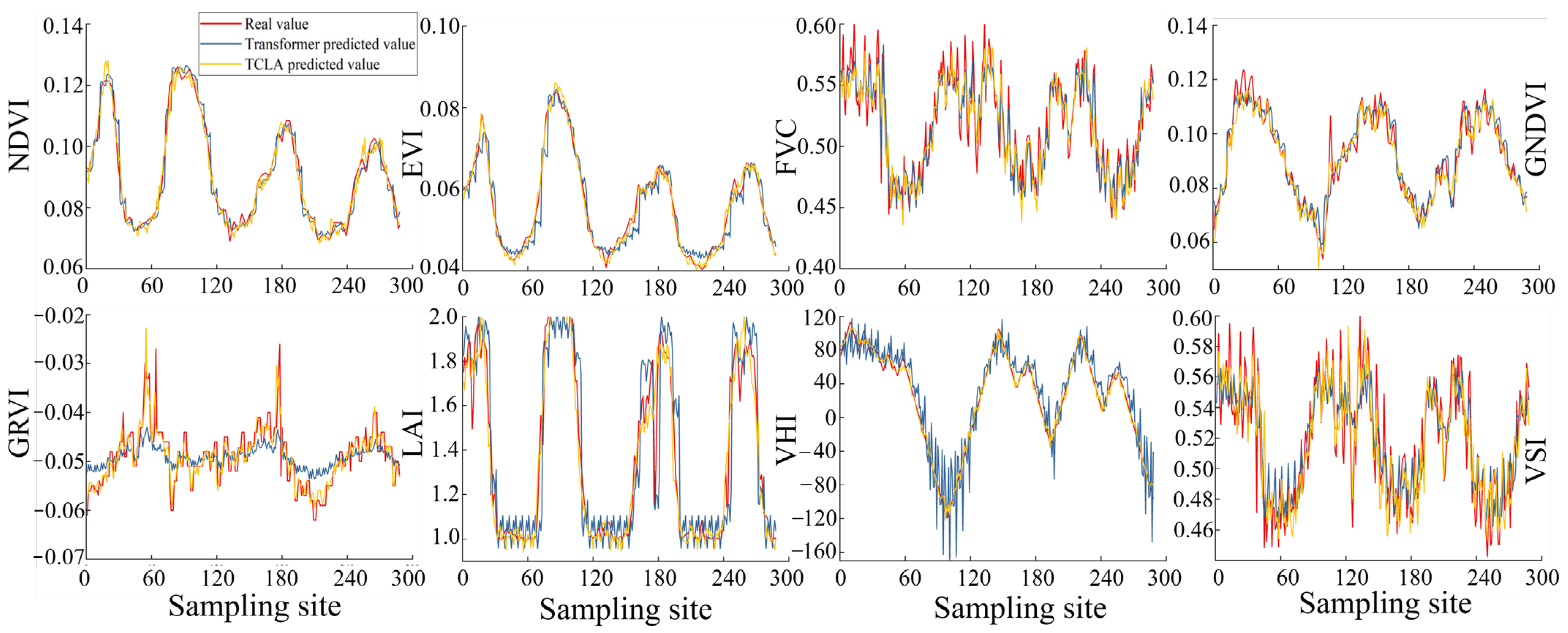
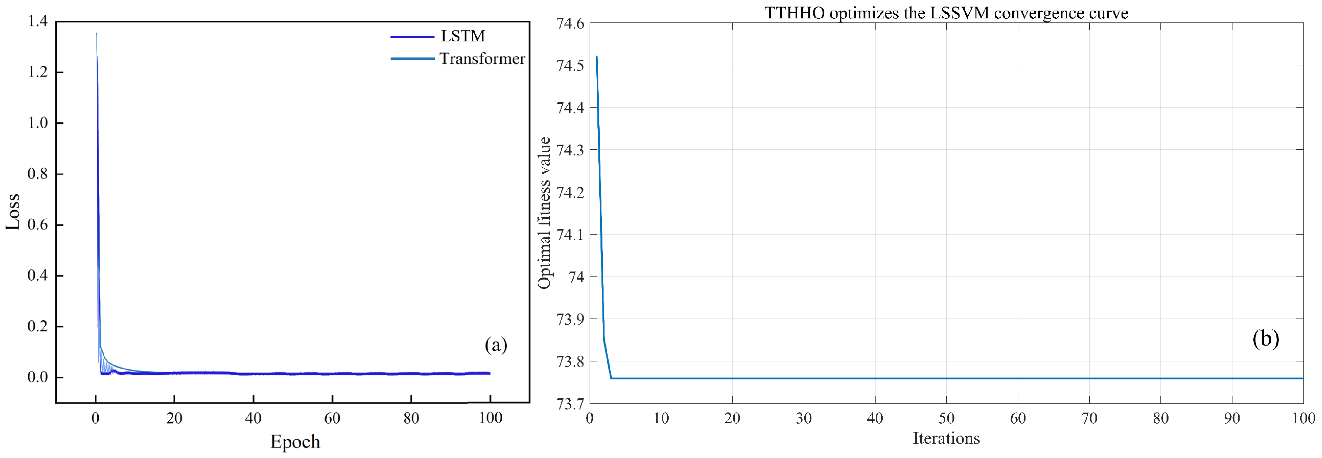
The TCLA model enhances prediction accuracy by 10.57% to 26.47% relative to traditional models (LSTM, Transformer), demonstrating superior generalization ability in managing complex datasets and effectively resolving the limitations of LSTM and Transformer models in high-dimensional and non-stationary data.

(2)

The multimodal TCLA model exhibits an overall accuracy enhancement of 3.57 ± 2.13% compared to single-modality models. The model exhibits optimal PINAW and PICP values performance, with negligible CRPS and CWC value variations. TCLA offers exact prediction intervals, a robust prediction distribution, and calibration stability.

(3)

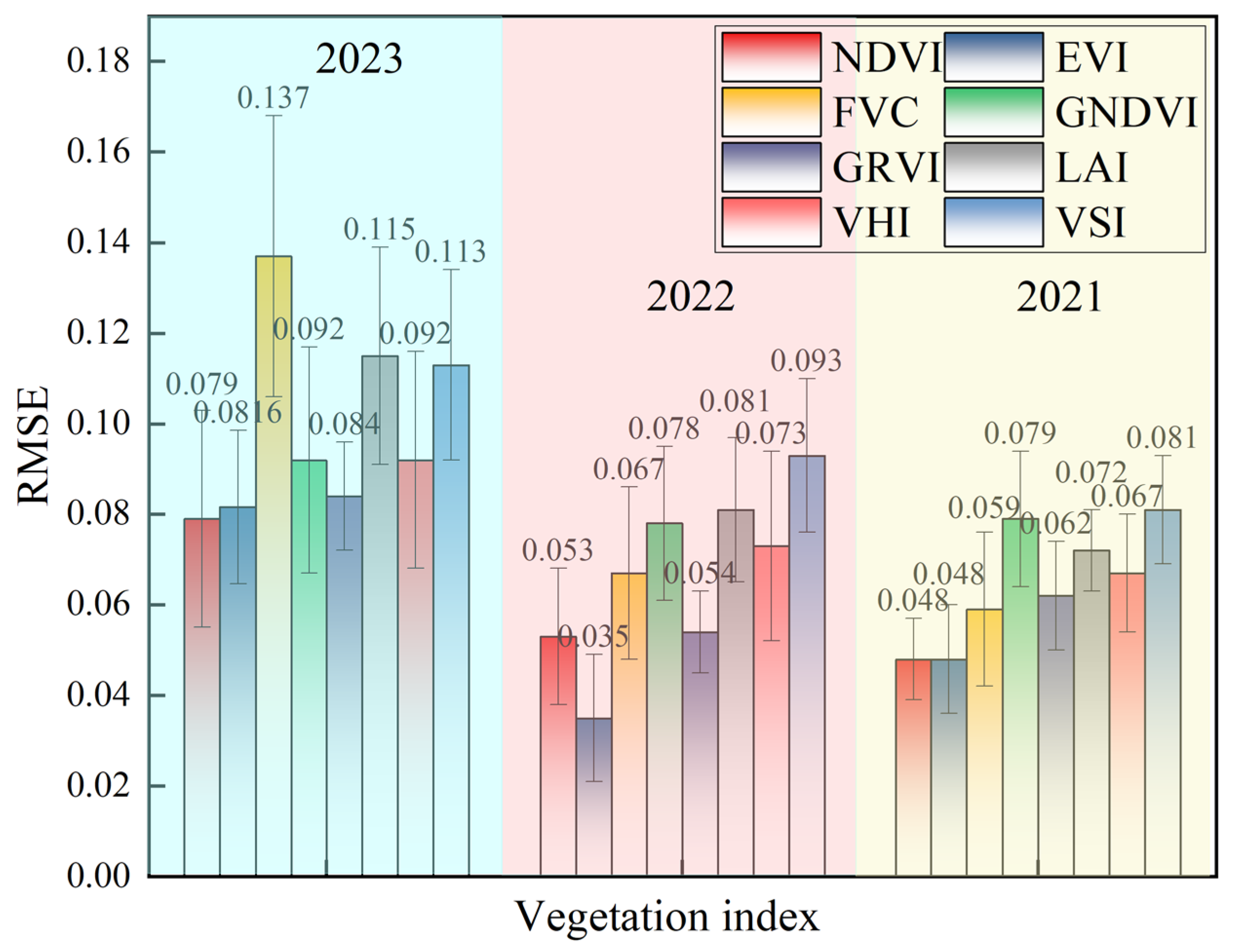
In the presence of outlier proportions between p₁ and p₃, the RMSE of the TCLA model diminishes by 45.18% to 69.66%, within a range of 0.079 to 0.137, thereby mitigating the influence of single-modality data and markedly enhancing the predictive accuracy.

Despite TCLA’s exceptional performance in accuracy and durability, its comparatively large computational complexity requires optimization. Future research will resolve critical challenges such as model complexity regulation, automated hyperparameter optimization, and enhancing interpretability to broaden the model’s application and significance, offering scientific backing for worldwide vegetation productivity monitoring.

References

1. De Lombaerde, E.; Vangansbeke, P.; Lenoir, J.; Van Meerbeek, K.; Lembrechts, J.; Rodríguez-Sánchez, F.; De Frenne, P. Maintaining forest cover to enhance temperature buffering under future climate change. Sci. Total Environ. 2022, 810, 151338. [Google Scholar] [CrossRef] [PubMed]
2. Blaga, L.; Ilieș, D.C.; Wendt, J.A.; Rus, I.; Zhu, K.; Dávid, L.D. Monitoring forest cover dynamics using orthophotos and satellite imagery. Remote Sens. 2023, 15, 3168. [Google Scholar] [CrossRef]
3. Ganjirad, M.; Bagheri, H. Google Earth Engine-based mapping of land use and land cover for weather forecast models using Landsat 8 imagery. Ecol. Inform. 2024, 80, 102498. [Google Scholar] [CrossRef]
4. Ball, J.G.; Petrova, K.; Coomes, D.A.; Flaxman, S. Using deep convolutional neural networks to forecast spatial patterns of Amazonian deforestation. Methods Ecol. Evol. 2022, 13, 2622–2634. [Google Scholar] [CrossRef]
5. Rana, M.; Sethuvenkatraman, S.; Goldsworthy, M. A data-driven approach based on quantile regression forest to forecast cooling load for commercial buildings. Sustain. Cities Soc. 2022, 76, 103511. [Google Scholar] [CrossRef]
6. Dupuy, F.; Mestre, O.; Serrurier, M.; Burdá, V.K.; Zamo, M.; Cabrera-Gutiérrez, N.C.; Oller, G. ARPEGE cloud cover forecast postprocessing with convolutional neural network. Weather Forecast. 2021, 36, 567–586. [Google Scholar] [CrossRef]
7. Walters, M.; Sinnett, D. Achieving tree canopy cover targets: A case study of Bristol, UK. Urban For. Urban Green. 2021, 65, 127296. [Google Scholar] [CrossRef]
8. Abdulrab, H.; Hussin, F.A.; Ismail, I.; Assad, M.; Awang, A.; Shutari, H.; Arun, D. Energy efficient optimal deployment of industrial wireless mesh networks using transient trigonometric Harris Hawks optimizer. Heliyon 2024, 10, e28719. [Google Scholar] [CrossRef]
9. Wei, F.; Feng, Y.; Shi, X.; Hou, K. Improved sparrow search algorithm with adaptive multi-strategy hierarchical mechanism for global optimization and engineering problems. Clust. Comput. 2025, 28, 215. [Google Scholar] [CrossRef]
10. Li, D.; Monteiro, D.D.G.N.; Jiang, H.; Chen, Q. Qualitative analysis of wheat aflatoxin B1 using olfactory visualization technique based on natural anthocyanins. J. Food Compos. Anal. 2025, 141, 107359. [Google Scholar] [CrossRef]
11. Shen, Y.; Wu, J.; Ma, M.; Du, X.; Niu, D. Application of an Improved Differential Evolution Algorithm in Practical Engineering. Concurr. Comput. Pract. Exp. 2025, 37, e8358. [Google Scholar] [CrossRef]
12. Shutari, H.; Ibrahim, T.; Nor, N.B.M.; Abdulrab, H.Q.; Saad, N.; Al-Tashi, Q. Coordination of enhanced control schemes for optimal operation and ancillary services of grid-tied VSWT system. IEEE Access 2023, 11, 43520–43535. [Google Scholar] [CrossRef]
13. Bala Krishna, A.; Saxena, S.; Kamboj, V.K. hSMA-PS: A novel memetic approach for numerical and engineering design challenges. Eng. Comput. 2022, 38, 3513–3547. [Google Scholar] [CrossRef]
14. Ali, H.H.; Fathy, A. Reliable exponential distribution optimizer-based methodology for modeling proton exchange membrane fuel cells at different conditions. Energy 2024, 292, 130600. [Google Scholar]
15. Su, Q.; Lu, H.; Yin, X.; Lu, Q.; Yan, J. Hybrid point-interval prediction method for stochastic dynamic response of subsea umbilical cable based on BO-BiLSTM and adaptive bandwidth KDE. Ocean Eng. 2025, 320, 120317. [Google Scholar] [CrossRef]
16. Cui, C.; Zhao, J.; Xu, M.; Xu, C.; Liu, H.; Wang, K. Multidimensional seismic fragility analysis of subway station structures using the adaptive bandwidth kernel density estimation and Copula function. Undergr. Space 2025, 22, 110–123. [Google Scholar] [CrossRef]
17. Li, J.D.; Sun, Y.Z.; Wang, X.C.; Yang, Q.; Liu, G.D.; Qie, H.T.; Li, F.X. Explainable machine learning for predicting mechanical properties of hot-rolled steel pipe. J. Iron Steel Res. Int. 2025, 18, 1–16. [Google Scholar] [CrossRef]
18. Zheng, G.; Li, K.; Yue, X.; Zhang, Y. A multifactor hybrid model for carbon price interval prediction based on decomposition-integration framework. J. Environ. Manag. 2024, 363, 121273. [Google Scholar] [CrossRef]
19. Chen, H.; Zheng, Y.; Huang, H.; Wang, Z.; Yang, B.; Ni, J. A point-interval prediction framework for minimum miscibility pressure of CO2-crude oil systems. Fuel 2025, 381, 133573. [Google Scholar] [CrossRef]
20. Liu, S.; Wang, Z.; Li, Y. A novel approach for multivariate time series interval prediction of water quality at wastewater treatment plants. Water Sci. Technol. 2024, 90, 2813–2841. [Google Scholar] [CrossRef]
21. Cao, Z.; Zhu, T.; Cai, X. Hydro-agro-economic optimization for irrigated farming in an arid region: The Hetao Irrigation District, Inner Mongolia. Agric. Water Manag. 2023, 277, 108095. [Google Scholar] [CrossRef]
22. Zhang, X.; Guo, P.; Zhang, F.; Liu, X.; Yue, Q.; Wang, Y. Optimal irrigation water allocation in Hetao Irrigation District considering decision makers’ preference under uncertainties. Agric. Water Manag. 2021, 246, 106670. [Google Scholar] [CrossRef]
23. Liu, Z.; Chen, Y.; Chen, C. Analysis of the spatiotemporal characteristics and influencing factors of the NDVI based on the GEE cloud platform and Landsat images. Remote Sens. 2023, 15, 4980. [Google Scholar] [CrossRef]
24. Hou, H.; Li, R.; Zheng, H.; Tong, C.; Wang, J.; Lu, H.; Wang, W. Regional NDVI Attribution Analysis and Trend Prediction Based on the Informer Model: A Case Study of the Maowusu Sandland. Agronomy 2023, 13, 2882. [Google Scholar] [CrossRef]
25. Shammi, S.A.; Meng, Q. Use time series NDVI and EVI to develop dynamic crop growth metrics for yield modeling. Ecol. Indic. 2021, 121, 107124. [Google Scholar] [CrossRef]
26. Meivel, S.; Maheswari, S.; Banu, D.F. Indices and Multispectral Images. In Proceedings of UASG 2021: Wings 4 Sustainability: Unmanned Aerial System in Geomatics; Springer: Berlin/Heidelberg, Germany, 2023; Volume 304, p. 343. [Google Scholar]
27. Yuan, Y.; Bao, A.; Liu, T.; Zheng, G.; Jiang, L.; Guo, H.; De Maeyer, P. Assessing vegetation stability to climate variability in Central Asia. J. Environ. Manag. 2021, 298, 113330. [Google Scholar] [CrossRef]
28. Štroner, M.; Urban, R.; Suk, T. Filtering green vegetation out from colored point clouds of Rocky terrains based on various vegetation indices: Comparison of simple statistical methods, support vector machine, and neural network. Remote Sens. 2023, 15, 3254. [Google Scholar] [CrossRef]
29. Qiao, K.; Zhu, W.; Xie, Z. Application conditions and impact factors for various vegetation indices in constructing the LAI seasonal trajectory over different vegetation types. Ecol. Indic. 2020, 112, 106153. [Google Scholar] [CrossRef]
30. Masoud, A.A. Hybrid wind-solar energy potential modeling using ERA5 and solar irradiation data in google Earth Engine. Renew. Energy 2024, 232, 121042. [Google Scholar] [CrossRef]
31. Givisiez, A.G.; Petrou, K.; Ochoa, L.F. A review on TSO-DSO coordination models and solution techniques. Electr. Power Syst. Res. 2020, 189, 106659. [Google Scholar] [CrossRef]
32. Silva, R.; Alves, E.; Ferreira, R.; Villar, J.; Gouveia, C. Characterization of TSO and DSO grid system services and TSO-DSO basic coordination mechanisms in the current decarbonization context. Energies 2021, 14, 4451. [Google Scholar] [CrossRef]
33. Kamboj, V.K.; Nandi, A.; Bhadoria, A.; Sehgal, S. An intensify Harris Hawks optimizer for numerical and engineering optimization problems. Appl. Soft Comput. 2020, 89, 106018. [Google Scholar] [CrossRef]
34. Wang, S.; Jia, H.; Abualigah, L.; Liu, Q.; Zheng, R. An improved hybrid aquila optimizer and harris hawks algorithm for solving industrial engineering optimization problems. Processes 2021, 9, 1551. [Google Scholar] [CrossRef]
35. Kattenborn, T.; Leitloff, J.; Schiefer, F.; Hinz, S. Review on Convolutional Neural Networks (CNN) in vegetation remote sensing. ISPRS J. Photogramm. Remote Sens. 2021, 173, 24–49. [Google Scholar] [CrossRef]
36. Kadkhodazadeh, M.; Farzin, S. A novel LSSVM model integrated with GBO algorithm to assessment of water quality parameters. Water Resour. Manag. 2021, 35, 3939–3968. [Google Scholar] [CrossRef]
37. Kamalov, F. Kernel density estimation based sampling for imbalanced class distribution. Inf. Sci. 2020, 512, 1192–1201. [Google Scholar] [CrossRef]
38. Moreo, A.; González, P.; del Coz, J.J. Kernel density estimation for multiclass quantification. Mach. Learn. 2025, 114, 92. [Google Scholar] [CrossRef]
39. Kong, Z.; Ling, H.; Deng, M.; Han, F.; Yan, J.; Deng, X.; Wang, W. Past and projected future patterns of fractional vegetation coverage in China. Sci. Total Environ. 2023, 902, 166133. [Google Scholar] [CrossRef]
40. Chen, M.; Xue, Y.; Xue, Y.; Peng, J.; Guo, J.; Liang, H. Assessing the effects of climate and human activity on vegetation change in Northern China. Environ. Res. 2024, 247, 118233. [Google Scholar] [CrossRef]
41. Cheng, M.; Jiao, X.; Liu, Y.; Shao, M.; Yu, X.; Bai, Y.; Jin, X. Estimation of soil moisture content under high maize canopy coverage from UAV multimodal data and machine learning. Agric. Water Manag. 2022, 264, 107530. [Google Scholar] [CrossRef]
42. Guan, Y.; Grote, K. Assessing the potential of UAV-based multispectral and thermal data to estimate soil water content using geophysical methods. Remote Sens. 2023, 16, 61. [Google Scholar] [CrossRef]
43. Zhang, M.; Tan, S.; Zhang, C.; Han, S.; Zou, S.; Chen, E. Assessing the impact of fractional vegetation cover on urban thermal environment: A case study of Hangzhou, China. Sustain. Cities Soc. 2023, 96, 104663. [Google Scholar] [CrossRef]
44. Qiu, S.; Miller, M.I.; Joshi, P.S.; Lee, J.C.; Xue, C.; Ni, Y.; Kolachalama, V.B. Multimodal deep learning for Alzheimer’s disease dementia assessment. Nat. Commun. 2022, 13, 3404. [Google Scholar] [CrossRef]
45. Venugopalan, J.; Tong, L.; Hassanzadeh, H.R.; Wang, M.D. Multimodal deep learning models for early detection of Alzheimer’s disease stage. Sci. Rep. 2021, 11, 3254. [Google Scholar] [CrossRef]
46. Yang, Y.; Wei, X.; Wang, J.; Zhou, G.; Wang, J.; Jiang, Z.; Ren, Y. Prediction of seedling oilseed rape crop phenotype by drone-derived multimodal data. Remote Sens. 2023, 15, 3951. [Google Scholar] [CrossRef]
47. Peng, X.; Ma, Y.; Sun, J.; Chen, D.; Zhen, J.; Zhang, Z.; Wang, Y. Grape leaf moisture prediction from UAVs using multimodal data fusion and machine learning. Precis. Agric. 2024, 25, 1609–1635. [Google Scholar] [CrossRef]
48. Peng, X.; Chen, D.; Zhou, Z.; Zhang, Z.; Xu, C.; Zha, Q.; Hu, X. Prediction of the nitrogen, phosphorus and potassium contents in grape leaves at different growth stages based on UAV multispectral remote sensing. Remote Sens. 2022, 14, 2659. [Google Scholar] [CrossRef]
49. He, F.; Zhang, S. Prediction of Ultra-Short Term Electricity Price Interval in Electricity Market Based on MIC-LSSVM-ABKDE. In International Conference of Electrical, Electronic and Networked Energy Systems; Springer Nature: Singapore, 2024; pp. 219–229. [Google Scholar]
50. Ezzaim, A.; Dahbi, A.; Aqqal, A.; Haidine, A. AI-based learning style detection in adaptive learning systems: A systematic literature review. J. Comput. Educ. 2024, 9, 1–39. [Google Scholar] [CrossRef]
51. Schilcher, J.; Nilsson, A.; Andlid, O.; Eklund, A. Fusion of electronic health records and radiographic images for a multimodal deep learning prediction model of atypical femur fractures. Comput. Biol. Med. 2024, 168, 107704. [Google Scholar] [CrossRef]
52. Dentamaro, V.; Impedovo, D.; Musti, L.; Pirlo, G.; Taurisano, P. Enhancing early Parkinson’s disease detection through multimodal deep learning and explainable AI: Insights from the PPMI database. Sci. Rep. 2024, 14, 20941. [Google Scholar] [CrossRef]
Figure 1. Study area. (a) Location of Dengkou in China. (b) Dengkou elevation. (c) Experimental site vegetation coverage and groundwater depth monitoring site.
Agronomy 15 01279 g001
Figure 2. TCLA model structure diagram.
Agronomy 15 01279 g002
Figure 3. TCLA model flowchart.
Agronomy 15 01279 g003
Figure 4. RLC exponential decay of voltage.
Agronomy 15 01279 g004
Figure 5. TTHHO algorithm structure diagram.
Agronomy 15 01279 g005
Figure 6. Performance comparison of TTHHO and HHO based on benchmark functions.
Agronomy 15 01279 g006
Figure 7. CNN model structure diagram.
Agronomy 15 01279 g007
Figure 8. LSSVM model structure diagram.
Agronomy 15 01279 g008
Figure 9. LSTM model: comparison of multiple vegetation indices between the training set and the test set.
Agronomy 15 01279 g009
Figure 10. Comparison of Transformer model and single-mode TCLA model in prediction accuracy of eight planting targets (NDVI, EVI, FVC, GNDVI, GRVI, LAI, VHI, VSI).
Agronomy 15 01279 g010
Figure 11. Model iteration process error comparison: (a) epoch error of LSTM and Transformer model within 100 times; (b) the optimum fitness value of the single-mode TCLA model over 100 iterations.
Agronomy 15 01279 g011
Figure 12. Correlation among multimodal data.
Agronomy 15 01279 g012
Figure 13. NDVI accuracy prediction and confidence interval of multimodal TCLA model.
Agronomy 15 01279 g013
Figure 14. Comparison between kernel density curves of different sampling points and actual values.
Agronomy 15 01279 g014
Figure 15. Model prediction results and residual analysis: (a) comparison of fundamental values and predicted values; (b) the residual of the model prediction error; (c) the distribution of residuals.
Agronomy 15 01279 g015
Figure 16. Kernel density estimation curves of prediction error under different bandwidth estimation methods.
Agronomy 15 01279 g016
Figure 17. The performance accuracy of the TCLA multimodal model under the condition of fewer outliers.
Agronomy 15 01279 g017
Figure 18. Evaluation of prediction accuracy for multi-modal and single-modal models with different outliers.
Agronomy 15 01279 g018
Figure 19. Prediction accuracy of vegetation factors in different years using the outlier-free TCLA multimodal model.
Agronomy 15 01279 g019
Figure 20. Testing the generalization capability of the TCLA multimodal model’s vegetation factors across different years and locations. (a) represents the first seven locations, (b) represents the remaining eight locations.
Agronomy 15 01279 g020
Figure 21. The importance of features predicted by the multimodal TCLA model as analyzed using the SHAP method (“Tem” stands for “temperature”, “Pre” stands for “precipitation”, “gd” stands for “groundwater depth”). (a) SHAP summary plot, (b) Mean absolute SHAP values (feature importance), (c) SHAP decision plot for EVI.
Agronomy 15 01279 g021