Article

Design and Implementation of an Intelligent Pest Status Monitoring System for Farmland

1
College of Engineering, Heilongjiang Bayi Agricultural University, Daqing 163319, China
2
College of Information and Electrical Engineering, Heilongjiang Bayi Agricultural University, Daqing 163319, China
*
Author to whom correspondence should be addressed.
Agronomy 2025, 15(5), 1214; https://doi.org/10.3390/agronomy15051214 (registering DOI)
Submission received: 26 April 2025 / Revised: 9 May 2025 / Accepted: 14 May 2025 / Published: 16 May 2025
(This article belongs to the Section Pest and Disease Management)

Abstract

:
This study proposes an intelligent agricultural pest monitoring system that integrates mechanical control with deep learning to address issues in traditional systems, such as pest accumulation interference, image contrast degradation under complex lighting, and poor balance between model accuracy and real-time performance. A three-axis coordinated separation device is employed, achieving a 92.41% single-attempt separation rate and 98.12% after three retries. Image preprocessing combines the Multi-Scale Retinex with Color Preservation (MSRCP) algorithm and bilateral filtering to enhance illumination correction and reduce noise. For overlapping pest detection, EfficientNetv2-S replaces the YOLOv5s backbone and is combined with an Adaptive Feature Pyramid Network (AFPN), achieving 95.72% detection accuracy, 94.04% mAP, and 127 FPS. For pest species recognition, the model incorporates a Squeeze-and-Excitation (SE) attention module and α-CIoU loss function, reaching 91.30% precision on 3428 field images. Deployed on an NVIDIA Jetson Nano, the system demonstrates a detection time of 0.3 s, 89.64% recall, 86.78% precision, and 1.136 s image transmission delay, offering a reliable solution for real-time pest monitoring in complex field environments.

1. Introduction

Agricultural pest infestations are one of the core threats to food security and crop yields [1,2,3]. Effective pest monitoring not only helps in the early detection of pest invasions but also provides accurate data to support the development of scientifically based pest control measures [4,5,6]. Traditional pest monitoring relies on manual inspections and chemical trapping devices, which suffer from low efficiency and high error rates [7,8,9]. With the modernization of agricultural production, deep learning-based visual detection technologies have provided a new approach for the automated monitoring of pests. Researchers have proposed various pest monitoring systems based on deep learning [10,11,12].
Lee et al. [13] proposed a deep learning-based citrus pest and disease automatic classification service system. The study established a multi-variable citrus image dataset, which was used to train transfer learning-based models, including VGGNet, ResNet, DenseNet, EfficientNet, and ViT, for citrus disease detection. The most effective EfficientNet model was then used to build a web application server capable of efficiently classifying citrus diseases. Azfar et al. [14] proposed an IoT-based cotton plant pest standard distortion correction formula and monitoring and intelligent response system. The system detected insects using motion detection sensors and triggered automatic responses through drone-based directional spraying. It covered the entire process of detecting cotton pests and responding to them, effectively eliminating pests with the help of drones and pesticides. Ali et al. [15] developed an IoT-based automatic pest monitoring system. The system utilized audio preprocessing techniques for pest sound analysis, collecting features and other statistical metrics from the sounds of 500 pest species, and trained, validated, and evaluated CNN, LSTM, Bi-LSTM, and CNN-Bi-LSTM models. Liu C and colleagues proposed a real-time field pest monitoring and early warning system based on deep learning. The system was designed with a dual-mode image acquisition device, using a light curtain sensor to trigger a high-speed camera for capturing free-falling pests. The system employed a Gaussian mixture model to achieve a 90.2% background removal rate.
A ResNet V2 deep learning model was built, and the experimental results on a standard laboratory dataset showed a detection accuracy of 96%, significantly outperforming traditional SVM (73.9%) and BPNN (75.0%). Using transfer learning and an indoor-field symmetric mixed dataset, the field data detection rate was improved to 84.6% and 85.7%, respectively [16]. Lippi et al. [17] proposed a data-driven monitoring system based on the YOLOv4 framework for the early detection of hazelnut gall mite pests in precision agriculture. The study optimized the model’s performance by integrating various data augmentation techniques and training it on two distinct seasonal datasets (spring and autumn). The system was tested for real-time performance on an embedded device, the NVIDIA Jetson Xavier. Čirjak et al. [18] developed an intelligent trap based on image analysis by integrating IoT and AI technologies. The system used convolutional neural networks (CNNs) for real-time species detection from moth trap images, achieving a detection accuracy of 96.9%. Additionally, infrared sensors and wingbeat frequency detection technologies were employed for automatic pest counting, with an accuracy near 100% for apple codling moth monitoring. The experimental results showed that compared to traditional manual monitoring, the system reduced the field inspection frequency by 60% and decreased pesticide use by 30% through real-time data warnings. The approach provided a precise management solution for the multi-generational and invasive pest issues caused by climate change.
Gao et al. [19] proposed a deep learning-based intelligent cotton pest and disease detection system by integrating Transformer technology and agricultural knowledge graphs, optimized for edge computing deployment. The system utilized data augmentation techniques to expand the dataset and combined a joint attention mechanism with a joint head design specifically tailored for small object detection to enhance feature detection capabilities. The system also built a structured knowledge graph incorporating pest and disease features and pest control knowledge, enhancing semantic understanding through feature embedding and model output fusion. A multi-source data alignment module was designed to integrate environmental sensor data, and local inference was achieved on mobile devices using the Core ML framework. Liu and colleagues [20] proposed an improved YOLOv4-based tomato pest detection system. The system optimized the feature extraction network CSPDarknet53 by integrating a triple attention mechanism, allowing the model to focus on key pest features. To address the class imbalance issue, the Focal Loss function was introduced to adjust the loss calculation, and K-means++ clustering was used to generate anchor boxes tailored to the size of the pests. The study constructed a labeled dataset containing four types of pests, including whitefly, aphids, leaf miners, and others, and enhanced the model’s generalization capability through data augmentation.
However, despite the theoretical advancements in pest monitoring systems, several challenges remain in practical applications [21,22,23]: (1) traditional pest trapping devices mostly rely on insecticidal lamps to attract and kill pests; these trapping devices lack the ability to separate overlapping pests, resulting in mixed image features and a 22–35% reduction in the average precision of detection models; (2) complex field lighting conditions, such as strong reflections or low illumination, degrade image contrast, making it difficult for the existing algorithms to reliably recover pest details; and (3) lightweight models deployed on edge devices face challenges in balancing accuracy and real-time performance. To address these issues, this study designs and develops a pest monitoring device that allows agricultural workers to obtain timely pest information and implement effective pest control measures.

2. Materials and Methods

2.1. System Architecture

The architecture of the intelligent pest detection system for farmland developed in this study is shown in Figure 1. The overall 12 v power is provided by solar photovoltaic (Mutual Wide Technology Corporation, Longyan, China). The system remotely collects pest images through a pest trapping device deployed in fields and uploads them to a cloud server via wireless transmission modules. A deep learning model is then applied to identify various types of pests within the images, enabling autonomous long-distance pest status analysis based on object detection techniques. The analysis results are instantly fed back to the staff, allowing them to monitor pest conditions in the fields in real-time and make timely pest management decisions based on the findings.

2.2. Design and Construction of the Pest Trapping Device

Traditional pest trapping devices mostly rely on insecticidal lamps to attract and kill pests. Once the pests are killed, they fall into a collection tray. However, the pests that accumulate in the tray can sometimes form clusters, which may lead to issues in the captured images. This can result in false negatives or false positives when the detection model analyzes the images. As a result, inaccurate pest status information may be obtained, leading to misjudgment and potential economic losses.
To address this issue, this study designed a pest separation device based on machine vision. This device can separate clustered pests after they are killed, capture images of the separated pests, and upload the images to a server for analysis.
The structure of the pest trapping and monitoring device developed in this study is shown in Figure 2. The main components include a frequency vibration insecticidal lamp (Jiaduo Science and Technology Ltd., Hebi, China), a partition plate, a ranging camera (Meisuoke Science and Technology Ltd., Shenzhen, China), stepper motors for axis control, a scraper, a pest collection box, a stepper motor for the partition, and a separation probe, among others. Based on its working principle, the device can be divided into two main functional modules: a pest trapping module and a pest separation module.
The pest trapping module is responsible for attracting and killing pests, while the pest separation module separates the accumulated pests and captures images of the separated pests. Both modules work in coordination to ensure the proper functioning of the pest monitoring system. The device is powered by a solar energy system, meeting the requirements for long-term use in unmanned environments.
Considering the typical activity height of pests [24,25,26] and the potential interference with data collection in field installations, the device is mounted at a height of 0.5 m above the ground. Upon activation, the pest trapping module begins operation, utilizing a frequency vibrating insecticidal lamp to attract and eliminate pests. This lamp employs a dynamically tuned combination of discrete light spectra that are sensitive to pest vision, enabling precise targeting. It is also equipped with a programmable frequency vibration module (0.1–100 Hz), which simulates key interspecific communication frequencies among pests to interfere with their behavior. This disrupts pest adaptation and helps maintain a consistently high trapping efficiency. The trapping cycle is set to two hours. After each cycle, the killed pests fall into a partition compartment. When the trapping cycle ends, a stepper motor drives the partition to open, allowing the pests to drop into a collection tray. Before the next cycle begins, the partition automatically closes. Upon completion of the trapping process, the pest separation module is activated. A pest overlap detection model deployed on an NVIDIA Jetson Nano development board is used to detect overlapping pests in the collection tray and determine the locations of overlapping regions. A range camera captures the spatial coordinates of these regions, which are then converted into two-dimensional coordinates. These coordinates are translated into electrical pulses by a microcontroller to control stepper motors, enabling precise separation of pest bodies. After separation, the system captures images of the pests and uploads them to a cloud server. A pest detection model on the server analyzes the images to identify pest species and count their numbers. The resulting data are transmitted to the client side, where staff can formulate targeted pest control strategies based on real-time pest status information.

2.3. Development of the Pest Separation Algorithm

2.3.1. Visual Localization Algorithm

This study proposed a dual-core heterogeneous architecture based on the NVIDIA Jetson Nano and STM32F407 platforms, adopting a hybrid scheduling strategy that combines preemptive priority and round-robin time slicing. This ensured the coordinated execution of motion control tasks and visual processing tasks. A monocular camera was mounted at the top of the device, facing downward for vertical imaging.
The visual localization component was constructed using an OV5647 camera (Xinleshi Technology Company, Shenzhen, China) with the following specifications: 5 megapixels, MIPI CSI-2 interface, 1080p at 30 fps. Due to the wide-angle lens, the OV5647 camera exhibits both radial and tangential distortions, which must be corrected through calibration. For this purpose, a 7 × 9 matte checkerboard calibration plate (with a square size of 30 mm × 30 mm) was employed, as illustrated in Figure 3.
A monocular camera was mounted vertically on the top of the device for image acquisition. The vision-based localization module was built using an OV5647 camera (5 MP, MIPI CSI-2 interface, 1080p, 30 fps) in conjunction with an NVIDIA Jetson Nano. Due to the wide-angle lens of the OV5647, both radial and tangential distortions were present. Radial distortion causes straight lines to appear curved, typically leading to barrel or pincushion effects. Tangential distortion arises from misalignment between the lens and the image sensor, resulting in image skew. If not corrected, these distortions introduce spatial inaccuracies that degrade the precision of coordinate mapping between the vision system and the mechanical execution system. Therefore, intrinsic calibration was required to eliminate such distortions.
The calibration procedure was as follows: a 7 × 9 matte checkerboard calibration board was used, with each square measuring 30 mm × 30 mm, covering a total area of 216 mm × 270 mm, as shown in Figure 3. The white circle in the upper left corner of the board was defined as the calibration origin (coordinate (0, 0)), with the X-axis extending horizontally to the right and the Y-axis extending vertically downward. The X-axis and Y-axis were aligned with the row and column directions of the image. Black squares were alternated with blue circular dots, positioned at the intersections between squares. The matte surface of the board helped reduce interference from ambient light reflections during image capture.
A total of 20 images were captured by adjusting the angle of the calibration plate to ensure coverage of the camera’s field of view, including edge regions and varying distances. During the acquisition process, external light interference was avoided to maintain image quality.
Subpixel corner detection was performed using the “Find Chessboard Corners” function in OpenCV 4.5.5, followed by refinement with the corner sub-pix function, which reduced corner localization error from ±1 pixel to ±0.1 pixel. A corresponding list of physical coordinates was generated, with the top left corner of the checkerboard defined as the origin.
Subsequently, the “cv2.calibrateCamera” function was used to compute the intrinsic matrix K (including focal lengths fx = 2916, fy = 2916, and principal point coordinates cx = 1296, cy = 972) and the distortion coefficients D (radial distortion: k = −0.2, k = 0.1; tangential distortion: p = 0.001, p = −0.002). Finally, the radial and tangential distortions were corrected using their respective distortion elimination formulas.
The radial distortion correction formula is:
x c o r r e c t e d = x 1 + k 1 r 2 + k 2 r 4 y c o r r e c t e d = y 1 + k 1 r 2 + k 2 r 4
The tangential distortion correction formulas are given as follows:
x c o r r e c t e d = x + 2 p 1 x y + p 2 ( r 2 + 2 x 2 ) y c o r r e c t e d = y + 2 p 2 x y + p 1 ( r 2 + 2 y 2 )
where x and y are the original normalized image coordinates, r2 = x2 + y2 is the squared radius from the optical center, and p1 and p2 are the tangential distortion coefficients.
An inverse mapping table was generated using “cv2.initUndistortRectifyMap”, and image rectification was performed using bilinear interpolation. After correction, the straightness error of the checkerboard lines was less than 0.1 pixels, and the distance error between adjacent circular markers was controlled within ±0.1 mm, as verified by a laser rangefinder. The root mean square (RMS) of the reprojection error from the calibration was 0.18 pixels. The maximum deviation in mapping to the mechanical coordinate system was 2.2 mm, primarily attributed to the measurement uncertainty of the camera installation height (H = 500 mm ± 0.5 mm).
After distortion correction, hand–eye calibration was performed to align the image coordinate system with the mechanical coordinate system. The objective of hand–eye calibration was to establish an accurate mapping between image coordinates and mechanical coordinates, ensuring that the actuator can move precisely to the target positions identified by the camera.
The hand–eye calibration procedure was as follows: four reference markers were fixed on the planar surface of the pest collection tray. A laser rangefinder was used to precisely measure their mechanical coordinates. A vertically mounted OV5647 camera, which was previously intrinsically calibrated (fx = 2916, fy = 2916, cx = 1296, cy = 972), captured images of the markers. The pixel coordinates of the markers were extracted using the “aruco.detectMarkers” function in OpenCV 4.5.5.
These pixel coordinates were then converted to world coordinates using the monocular distance estimation formula:
X w = u c x f x ,   Y w = v c x · H f y
where u and v represent the position of the target in the image and H is the camera height (set to 500 mm).
Since the mapping from the image coordinate system to the mechanical coordinate system is an affine transformation, it was necessary to construct an affine transformation equation, as shown in the following formula. The parameters of the equation can be solved using the least squares method:
X m Y m = a b c d X w Y w + t x t y
The Equation (4) can be expanded as:
X m = a X w + b Y w + t x Y m = c X w + d Y w + t y
where a and d are the scaling factors in the mechanical coordinate system; b and c represent the deformation of the mechanical coordinate system; tx is the offset of the world coordinate system origin along the Xm direction of the mechanical coordinate system; and ty is the offset of the world coordinate system origin along the Ym direction of the mechanical coordinate system. In practical applications, the target world coordinates (35.0, 4.8) mm can be mapped to the mechanical coordinates (37.2, 3.3) mm through the affine transformation. The converted coordinates were then used to generate electrical pulses, driving the actuator to move to the target position.

2.3.2. Machine Motion Control Algorithm

The motion control algorithm of this system is based on a three-axis coordinated driving architecture, integrating kinematic modeling, closed-loop feedback control, and adaptive fault tolerance strategies. As shown in the gantry structure diagram, the core of the system hardware consists of three 42BYGH34 stepper motors and their synchronous belt drive mechanisms:
The X-axis (horizontal motion axis) employs a ball screw with a lead of 10 mm, coupled with a half-step driving mode (800 steps per revolution), achieving a single-step displacement resolution of 0.0125 mm. The motion range spans from 0 to 300 mm, with a maximum speed of 150 mm/s.
The Y-axis (vertical motion axis) transmits the motor output torque to a lead screw with a lead of 5 mm via a synchronous belt drive system. In full-step mode (1600 steps per revolution), the effective lead is corrected to 10 mm, resulting in a resolution of 0.00625 mm per step.
The Z-axis (vertical motion axis) directly drives a ball screw with a lead of 5 mm, achieving a resolution of 0.003125 mm per step in full-step mode. This axis works in conjunction with the separation probe to perform precise downward pressing operations.
After determining the location of the overlapping regions, the motion control algorithm uses a discrete pulse distribution to achieve multi-axis linkage:
The pulse count NX corresponding to the X-axis displacement ΔX is calculated as NX = ΔX/0.0125, and the pulse count NY corresponding to the Y-axis displacement ΔY is calculated as NY = ΔY/0.00625. The pulse frequency ratio between the two axes is strictly maintained at 2:1 to ensure the precision of linear interpolation.
The downward pressing stroke ΔZ is calculated as NZ = ΔZ/0.003125 and combined with an S-curve velocity profile to achieve smooth contact. The acceleration curve function is given by:
a t = 1 2 j m t 2 0 t < t 1 a t = a m a x t 1 t < t 2 a t = a m a x 1 2 j m t 2 ( t t 2 ) 2 ( t 2 t < t 3 )
where jm represents the rate of change in acceleration; amax is the maximum allowable acceleration of the motor; t1 is the time required for acceleration to increase from zero to amax; t2 is the duration for which the motor maintains the maximum acceleration amax; and t3 is the time for acceleration to decrease from amax to zero.
The acceleration rate jm is set to 5000 mm/s3, and the maximum acceleration amax is set to 200 mm/s2. These parameters effectively suppress probe impact, thereby preventing pest displacement.
The pressure closed-loop control module achieves precise force adjustment through current feedback. When the probe contacts the pest, the STM32F407 microcontroller samples the current signal from the motor driver chip at a frequency of 10 kHz. The signal is then converted by a 12-bit ADC and fed into a PID controller:
u k = K p e k + K i i = 0 k e ( i ) T s + K d e k e ( k 1 ) T s
where Kp is the proportional gain, determining the direct influence of the current error on the control output; Ki is the integral gain, used to eliminate steady-state error; TS is the time interval between two control cycles; and Kd is the derivative gain, used to suppress the rate of error change and improve system stability.
For complex adhesion cases, the system employs a three-level adaptive retry strategy, as shown in Figure 4. Separation failure is defined when the overlapping area detected by vision exceeds 80% or the current peak is below 1.0 A. Upon the first separation failure, uniform random disturbances are introduced within a ±0.3 mm range around the target position in both the X-axis and Y-axis (ΔX∼U (−0.3,0.3), ΔY∼U (−0.3,0.3)), and the pressure is increased to 0.7 N. In the second retry, the disturbance range is expanded to ±0.5 mm, and the pressure is increased to 0.9 N. If the separation still fails, a spiral path scraping mode is activated, where the probe follows an Archimedean spiral trajectory.
X k = X t + 0.2 k c o s 0.4 π k Y k = Y t + 0.2 k s i n 0.4 π k
where Xt represents the center position of the overlapping pest bodies detected by the vision system. The coordinates (Xt, Yt) serve as the geometric center of the spiral path, ensuring that the scraping motion always occurs around the target area; 0.2k is the instantaneous radius of the spiral path; and 0.4πk is the instantaneous angle of the spiral path.
k represents the number of scraping turns. With each increase of 1 in k, the radius of the spiral path expands by 0.2 mm, gradually increasing the scraping range of the separation probe. If all three retries fail, the system performs an emergency rollback operation: the Z-axis lifts by 20 mm with an acceleration of 200 mm/s2, and the X/Y axes move in reverse along the motion trajectory back to the origin. An alarm command is then sent via the UART protocol.
The experimental results show that the machine achieves a single separation success rate of 92.41% on the standard test board (3D-printed pest model). After three retries, the cumulative success rate increases to 98.12%.

2.4. Image Processing

In order to better simulate the environment of overlapping pest detection and ensure the diversity of experimental sample data, pest images were captured using a smartphone. The image acquisition took place in the experimental field of the Baiyi Agricultural University in Heilongjiang, China, in July 2023, resulting in a total of 2367 pest images.
Most of the images captured with the smartphone contained individual pests, which did not meet the requirements for overlapping clusters. Therefore, a Copy–Paste data augmentation technique was applied to simulate the overlapping accumulation of pests in real-world scenarios.
Additionally, since the photos were taken at different times, natural light intensity variations also affected the quality of the pest images. Excessive lighting could reduce the image contrast, making the image appear blurry, while insufficient lighting could make it difficult to distinguish details and lead to the loss of important feature information. Directly using such images would compromise the detection accuracy of the model. To address this issue, the Multi-Scale Retinex with Color Restoration (MSRCP) algorithm was applied to enhance the images by correcting uneven illumination and restoring color fidelity. The MSRCP algorithm, based on Retinex theory, simulates how the human eye perceives color while ignoring the effects of uneven lighting. Compared with traditional multi-scale Retinex algorithms, the MSRCP algorithm introduces a color restoration factor, which improves the restoration of color information. This improvement makes MSRCP more effective in maintaining natural color and rich details in images under uneven lighting conditions. However, images enhanced with MSRCP may have halos and noise, so bilateral filtering was used in this study to remove halos and noise from the images.
To compare the effects of different image enhancement techniques, this study compared the results of MSRCP enhancement alone and the combined use of MSRCP and bilateral filtering. The comparison results are shown in Figure 5. As seen in the figure, in the pest images captured under strong sunlight, the contrast between the pest bodies and the background, as well as between different pests, is not apparent. In images taken in outdoor environments with insufficient lighting, the details of pest bodies are blurred, causing the loss of many key features. After color reconstruction with the MSRCP algorithm, the images with abnormal brightness were corrected, and the brightness returned to normal, while the image saturation was enhanced. For the images with excessively high brightness, the outlines of the pests became more prominent after processing with the MSRCP algorithm. For the images with insufficient brightness, the pest features became clearer under the MSRCP algorithm. As shown in Processing 1 in Figure 5, the images processed with MSRCP have noticeable noise. In Processing 2, after applying bilateral filtering, although some details of the image were lost, the salt-and-pepper noise was significantly reduced, effectively simplifying the background of the image. In summary, the combination of the MSRCP algorithm and bilateral filtering can effectively solve the issue of image quality degradation due to environmental lighting variations.
Due to the limited number of pest images in the dataset, data augmentation techniques, such as scaling and flipping, were applied to the original images to reduce the risk of overfitting caused by insufficient training samples. After data augmentation, a total of 4000 overlapping pest images were obtained. The dataset was then divided into training and validation sets in a 9:1 ratio.
In this study, pest images captured in the field were used to construct the experimental dataset. The primary pest categories collected included lepidopteran borers, beetles, and flies. After screening, 3428 images were selected as the raw dataset, with the specific pest species and their quantities detailed in Table 1. Following image enhancement, the dataset was expanded to 1600 images per pest category. To mitigate the impact of uneven illumination on image quality, the MSRCP algorithm was applied in combination with bilateral filtering to enhance the original images.
To prevent overfitting due to the small size of the dataset, data augmentation techniques, such as horizontal and vertical flipping, brightness enhancement, brightness reduction, and adding salt-and-pepper noise, were employed to expand the dataset. After augmentation, a total of 16,000 images were obtained, which were then divided into training and testing sets in a 9:1 ratio.

2.5. Construction of the Overlapping Pest Detection Model

2.5.1. Algorithm Selection

In this study, the YOLOv5 model was selected as the baseline model. YOLOv5 is the fifth iteration in the YOLO series, with significant improvements over YOLOv4 that enhance both speed and accuracy. The model’s architecture can be divided into four main components: the input, the backbone network, the neck, and the head.
The backbone network begins by extracting features: the Focus structure compresses image slices while expanding the number of channels; the Cross Stage Partial (CSP) module performs staged extraction of multi-level features efficiently; and the Spatial Pyramid Pooling (SPP) module enhances the receptive field through multi-scale pooling operations. The neck employs the PANet structure, which integrates deep semantic and shallow detailed features through a bidirectional feature pyramid (bottom-up and top-down), improving the detection capability for multi-scale objects, especially small targets. Finally, the head performs multi-scale predictions across different feature maps, outputting the object location, class, and confidence. Non-Maximum Suppression (NMS) is then used to eliminate redundant bounding boxes, achieving high-precision detection.

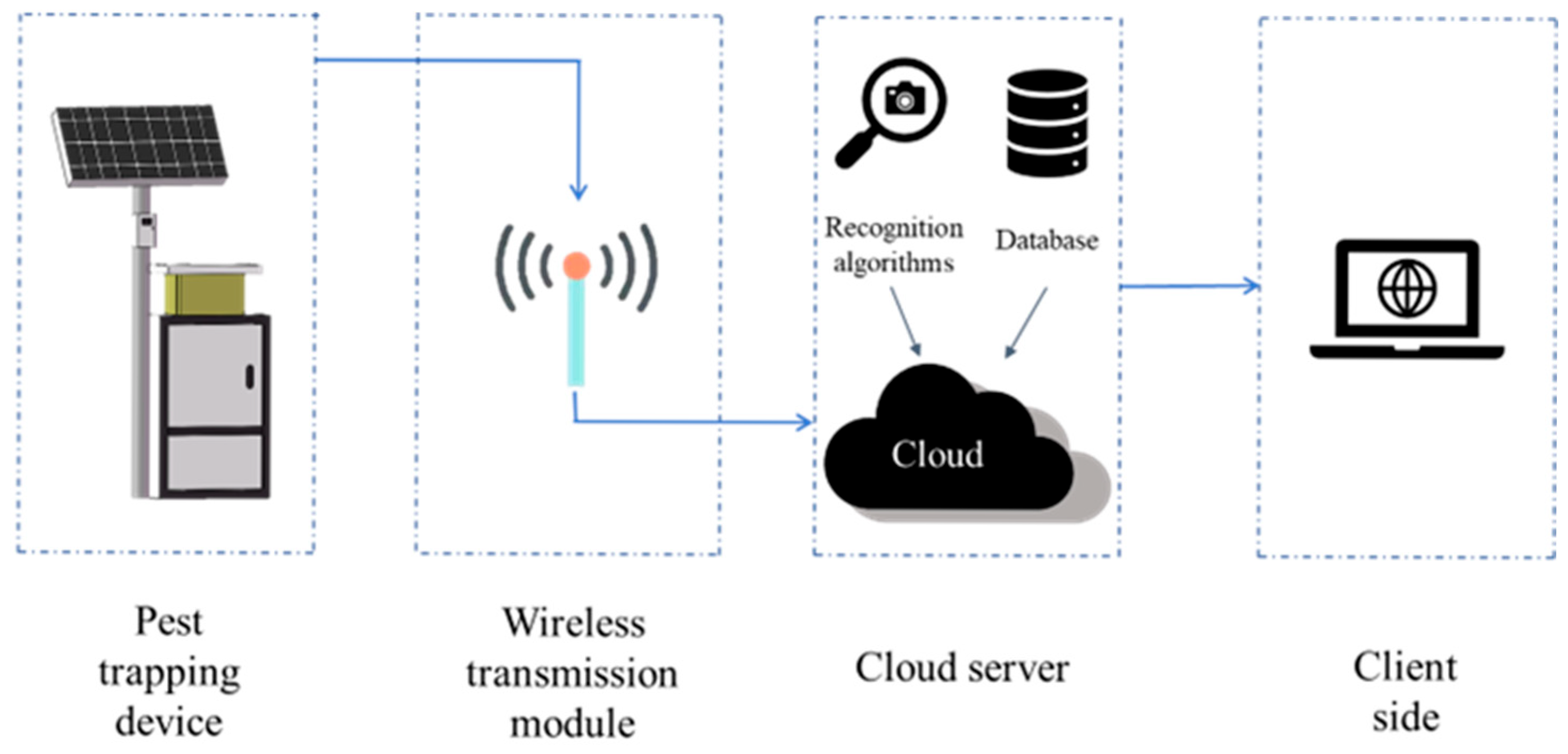
2.5.2. Algorithm Improvement

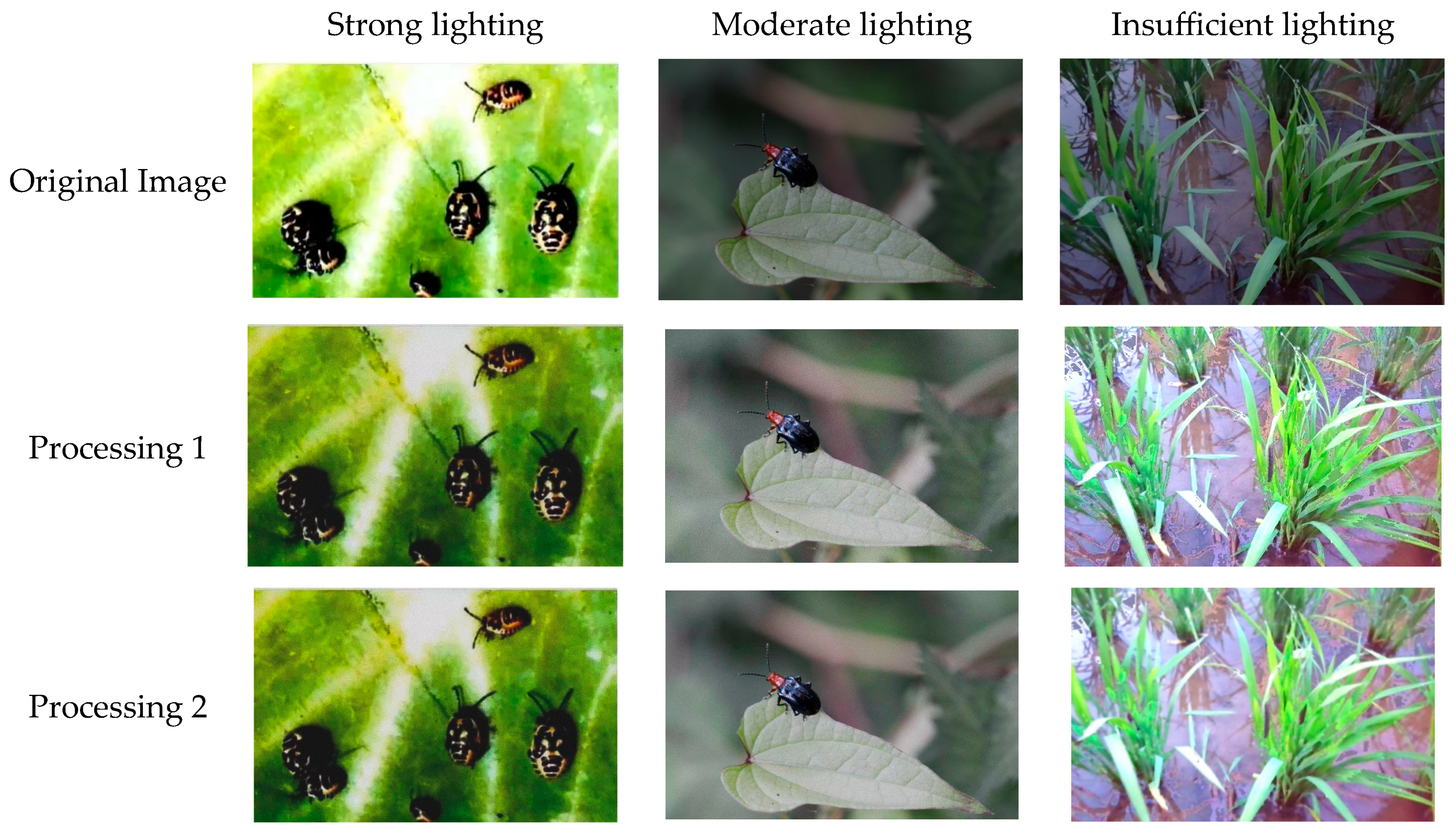
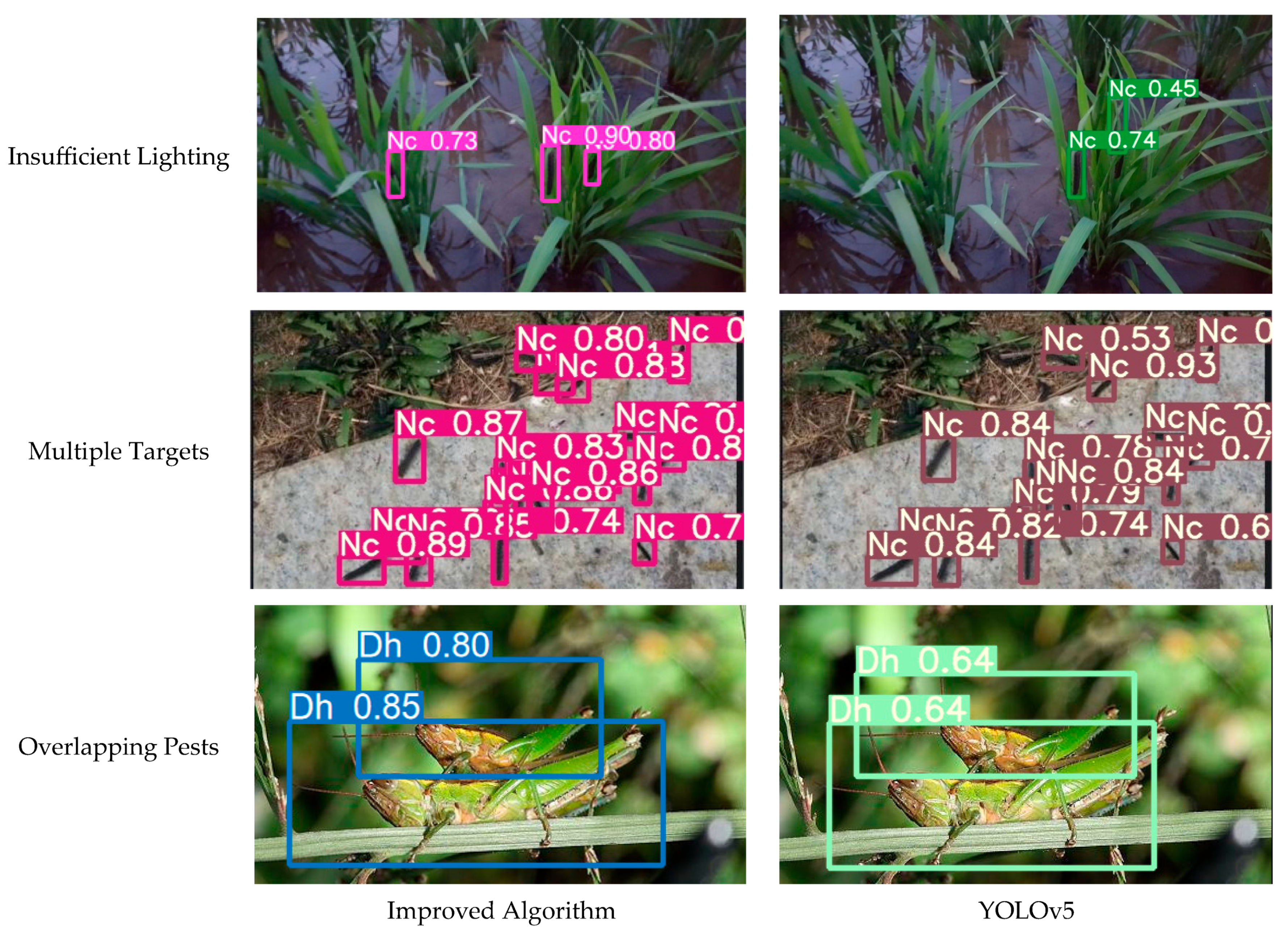
Although the impact of uneven lighting on the collected overlapping pest images was corrected using the MSRCP algorithm, there still exist near-field interference sources, such as soil particles and crop residues. Additionally, due to the local similarity in the texture and appendage features of the pests, there is a risk of feature confusion, which can lead to false detections. Furthermore, due to the limitations of the smartphone’s shooting angle and depth of field variations, along with the 3D stacking effect during pest aggregation, traditional methods face a risk of missing detections when identifying the morphological continuity of partially occluded pests.
To address these issues, this study replaced the YOLOv5 backbone network with EfficientNetv2-S while retaining the Spatial Pyramid Pooling-Fast (SPPF) structure. The Convolutional Block Attention Module (CBAM) was introduced as a hybrid attention mechanism to enhance the response weights of pest-related features, such as antenna textures and intersegmental connections. Additionally, the Adaptive Feature Pyramid Network (AFPN) was employed to construct multi-scale adaptive fusion pathways, improving the representation of overlapping targets through adaptive cross-scale feature interactions.
(1)
Replacing the Backbone Network.
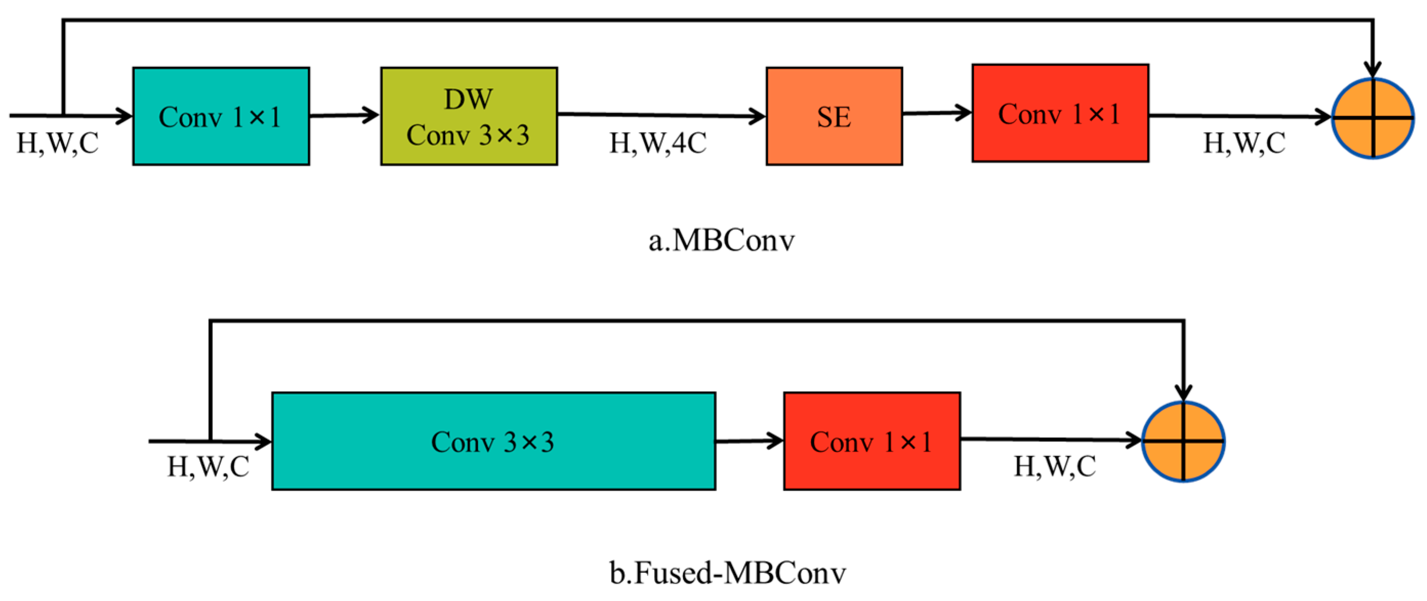
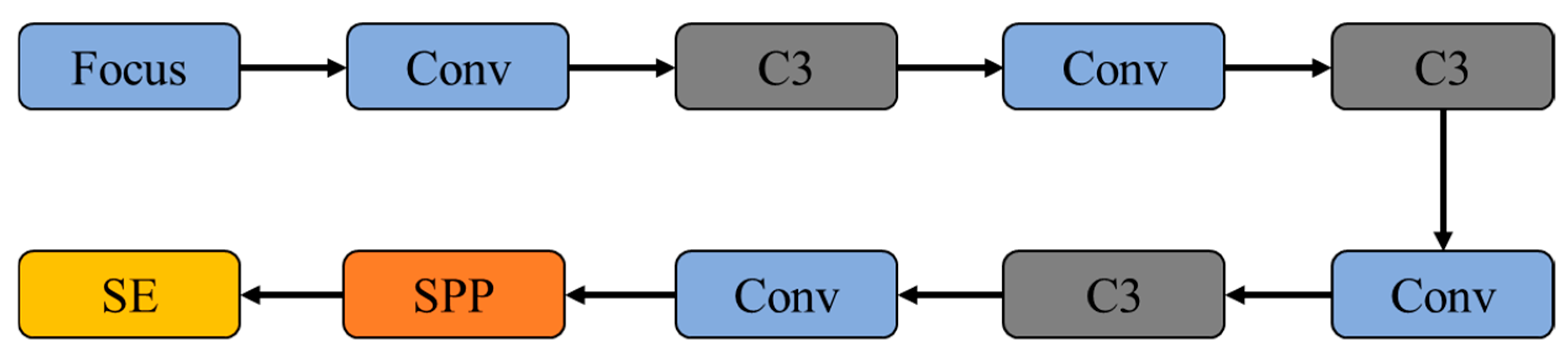
Due to the limited computational power of the NVIDIA Jetson Nano development board, the model was optimized for lightweight processing by replacing the backbone network with the EfficientNetv2-S lightweight network.
Compared to the EfficientNetv1 network, EfficientNetv2 replaces the shallow-layer MBConv with Fused-MBConv, which combines the 1 × 1 convolution and 3 × 3 depthwise convolution in MBConv into a single standard 3 × 3 convolution. This optimization fully utilizes GPU performance. Additionally, a progressive scaling strategy and optimized training methods were introduced, significantly improving training speed and inference efficiency.
The EfficientNetv2 series includes three model variants: S, M, and L. The S version serves as the base architecture, while M and L variants achieve performance gains by increasing the structural complexity, but this also requires more computational resources. Considering the balance between model efficiency and device computational capacity, this study selected the EfficientNetv2-S as the optimal solution for the backbone network due to its computational cost efficiency. The detailed structure of EfficientNetv2 is shown in Figure 6.
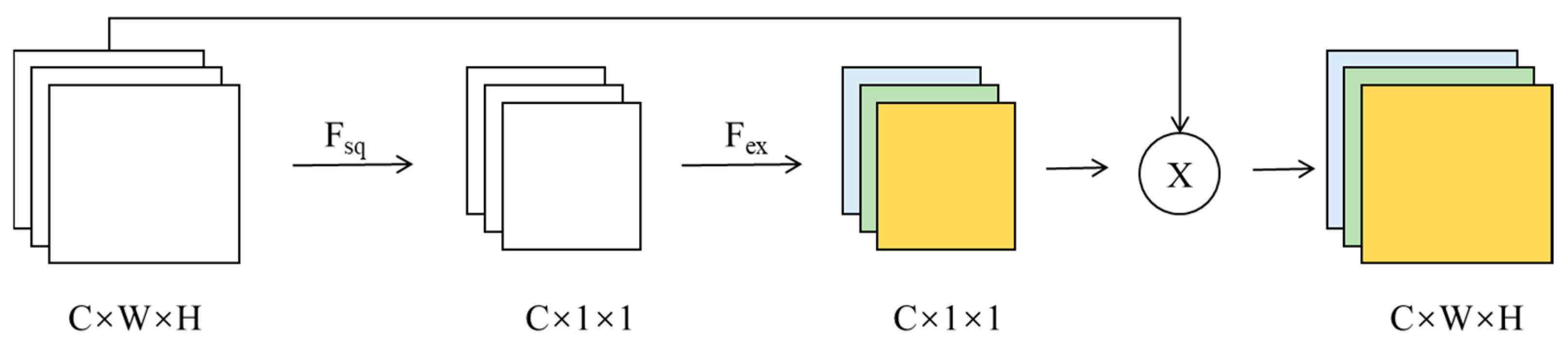
The SE module was used to enhance the network’s channel feature extraction capabilities. However, in the actual network construction, the Fused-MBConv in shallow layers did not use the SE module, while the MBConv in deeper layers incorporated the SE module. This is because, in shallow layers with fewer channels, the computational overhead of the SE module is relatively high, and the benefits are limited.
(2)
Adding the CBAM attention mechanism.
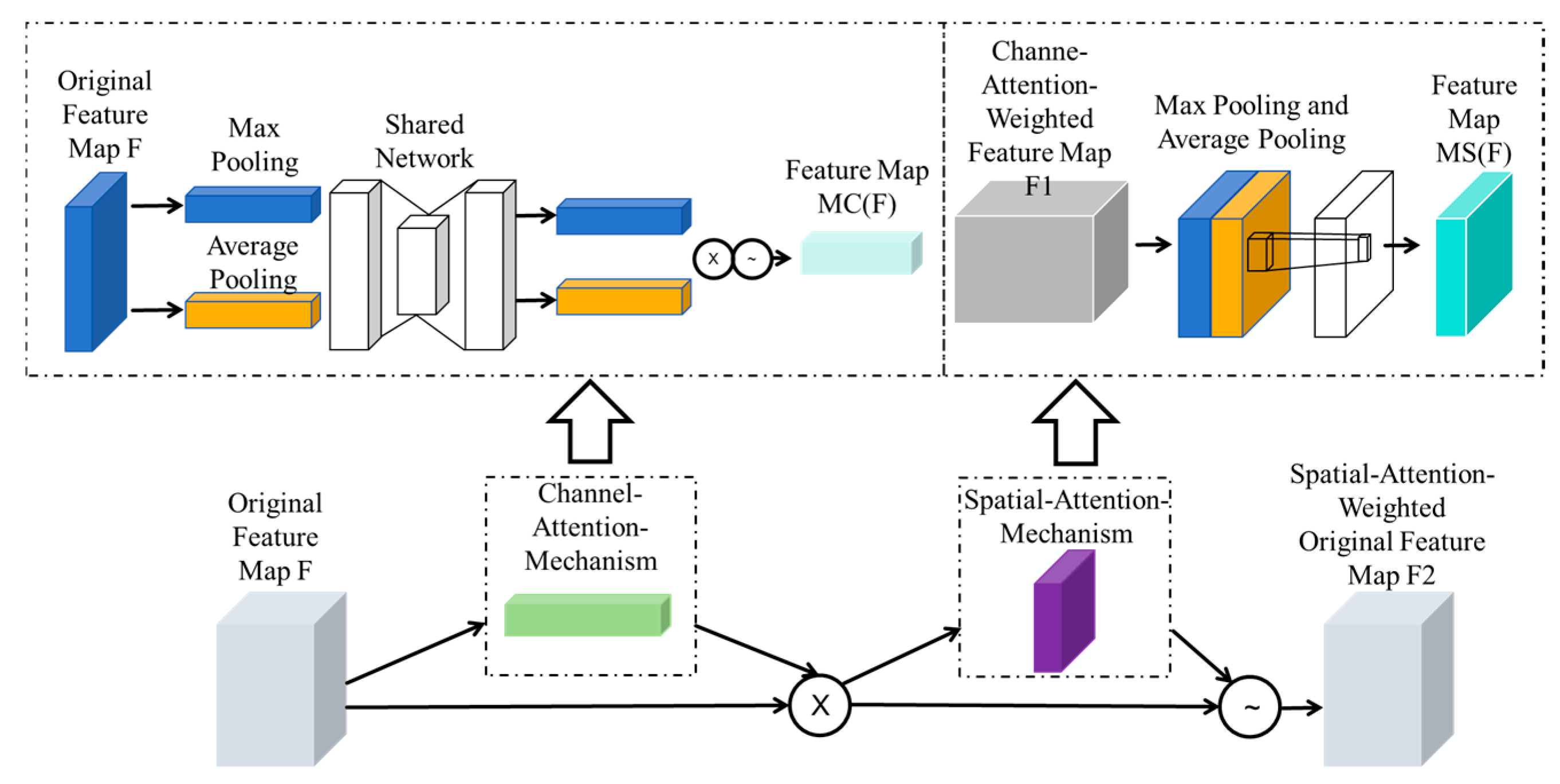
To improve detection performance in overlapping pest detection, which is hindered by overlapping pest body shapes, low-contrast features, and multi-scale interference, the CBAM (Convolutional Block Attention Module) attention mechanism employed a channel-space dual-branch weight recalibration strategy. By adding the CBAM attention mechanism before the SPPF, the model was optimized.
The channel attention module generates channel weight vectors using global average pooling and a multi-layer perceptron, selectively enhancing the channel dimensions corresponding to the morphology and high-frequency textures of overlapping pest bodies while suppressing interference from background channels with similar colors. The spatial attention module constructs a spatial weight matrix through max pooling and convolution operations, strengthening the spatial activation of key pest features (e.g., the base of the antenna and segmental connections) in overlapping areas. This spatial domain recalibration enhances the gradient response of these critical features.
The structure of the CBAM attention mechanism is illustrated in Figure 7.
(3)
Replacing PANet with the AFPN Structure.
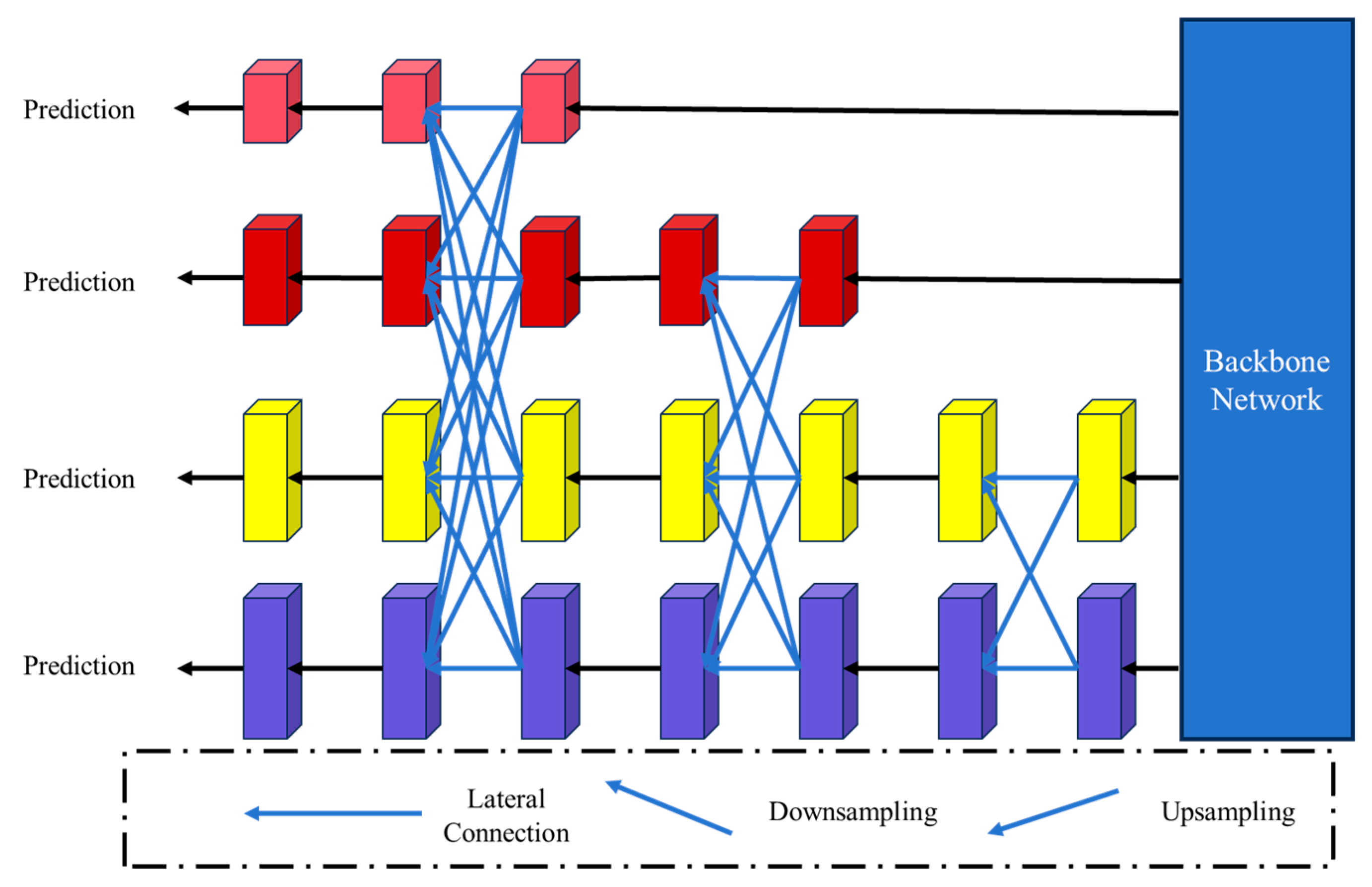
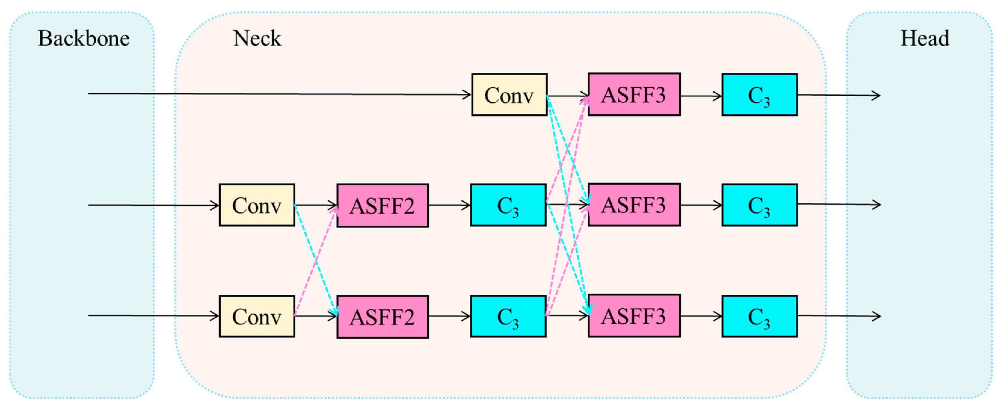
In the task of overlapping pest detection, feature confusion arises due to the dense accumulation of pest bodies, significant scale differences, and blurred anatomical details. To address this issue, the Neck layer of YOLOv5 was topologically restructured: the original PANet was replaced with the Adaptive Feature Pyramid Network (AFPN). The core improvement in AFPN lies in establishing an asymmetric interaction mechanism for multi-level features, as shown in Figure 8.
Traditional FPN/PANet uses a linear bidirectional fusion strategy, which overlooks the heterogeneous contribution of features at different resolutions to overlapping pest detection tasks. This was especially problematic when processing low-resolution images in the dataset, as the high-frequency texture features of small-scale pests are easily overwhelmed by the large-scale background noise. As a result, PANet suffers from inadequate feature fusion, semantic information loss, and the degradation of fine details, ultimately affecting detection accuracy and robustness. To address this limitation, this study introduced the Adaptive Feature Pyramid Network (AFPN) to replace PANet in YOLOv5, as illustrated in Figure 9.
ASFF2 to ASFF3: The specific structure of adaptive spatial feature fusion (ASFF). In the multilevel feature fusion process, ASFF technique is used to match the spatial weights of features at different levels and to adjust the influence of features at different levels so as to increase the importance of the key layers and to reduce the information conflicts from different layers.
As shown in Figure 8, AFPN optimizes multi-scale information fusion through a hierarchical feature integration mechanism. During the feature generation process from bottom to top in the backbone network, an incremental fusion strategy is employed: first, shallow high-resolution features are integrated, followed by the fusion of middle-level semantic features, and finally, high-level features are incorporated.
Due to significant semantic differences between non-adjacent layers (e.g., bottom and top layers), cross-layer connections in traditional pyramid networks often lead to feature exclusion. AFPN innovatively introduces a dynamic spatial weight allocation module (indicated by the blue connection lines in the figure). This module constructs a feature importance evaluation matrix through a learnable spatial attention mechanism, achieving optimization in three aspects:
Differentiated spatial weight allocation: High weight coefficients are assigned to low-level detail features (e.g., pest appendage contours), while the weight of high-level abstract features is adaptively adjusted according to background complexity.
Conflicting signal suppression: A channel-space dual-dimension calibration is used to eliminate response conflicts between cross-layer feature maps.
Key feature enhancement: Spatial pyramid pooling is used to strengthen the structural significance of pest bodies.
This design, through the coordinated operation of lateral connections (cross-resolution feature bridging), downsampling (spatial information compression), and upsampling (detail restoration), significantly improves the feature separability of overlapping pest targets.

2.6. Construction of the Pest Detection Model

This study applied the YOLOv5s model to agricultural pest detection, employing a transfer learning strategy to train the model. The following improvements were made to the model: first, an enhancement in pest feature extraction by adding the SE attention mechanism to the backbone network; second, a modification of the loss function during the network training process, replacing the CIoU loss function in YOLOv5 with Alpha-IoU.
The agricultural pest detection and counting algorithm model was deployed on an Alibaba Cloud server in this study, establishing data communication between the server and client. Additionally, a NoSQL database, MongoDB, was used for internal data storage and management.

2.6.1. SE Attention Mechanism

By applying the attention mechanism, deep learning models can more accurately capture the structural characteristics and semantics of input data. When processing visual information, the attention mechanism enables the model to focus on the key parts of the input data, allowing for a deeper understanding of the image content and enhancing the model’s interpretability. Therefore, specific attention mechanisms can be utilized to process important information in agricultural pest detection.
The SE attention mechanism, as a lightweight attention mechanism, is plug-and-play with a simple structure, as shown in Figure 10. Although the SE module introduces additional channel-wise operations, these operations are lightweight and do not significantly increase the computational burden relative to the overall model. By directly revealing the interdependencies between channels, it significantly enhances the model’s expressive power, enabling it to handle complex input data more effectively.
The SE attention mechanism consists of two key operations: squeeze and excitation. The squeeze operation uses a global average pooling layer to compress the feature map of each channel into a scalar value, resulting in a global feature descriptor. This operation effectively integrates global contextual information, allowing the network to capture the global dependencies between channels. The formula for the squeeze operation is as follows:
Z c = F s q ( u c ) = 1 H × W i = 1 H j = 1 W u c i , j
where H, W, and C represent the height, width, and number of channels of the image, respectively; uc denotes the output of size H × W × C; and zc is the output after compression, resulting in a 1 × 1 × C output.
The excitation operation consists of two fully connected layers. The first fully connected layer uses the ReLU activation function, which retains positive inputs and sets negative inputs to zero, thereby performing nonlinear feature transformation and selection. The second fully connected layer uses the Sigmoid function to normalize the channel values to the range (0, 1). This value represents the proportion of each channel’s contribution to the final weight, resulting in the activation values of the channels. These activation values reflect the model’s attention to each channel’s features. Through subsequent operations, the weights adjust the contribution of each channel. The formula for the excitation operation is as follows:
s = F e x ( z , W ) = σ W 2 δ W 1 z
where W1 is the dimensionality reduction matrix; W2 is the dimensionality expansion matrix; δ is the ReLU activation matrix; σ is the Sigmoid activation matrix; z is the channel feature vector after the squeeze operation; and s is the channel weight vector generated after the excitation operation.
To enhance the model’s focus on channel information, this study added the SE attention module to the backbone network of the YOLOv5 model, as shown in Figure 11. This modification constructed feature mappings based on inter-channel relationships, increasing the weight of useful information within the feature layers. As a result, the detection accuracy of pest species was improved, and the probability of false detections during model inference was reduced.

2.6.2. Training Strategy

During model training, a transfer learning strategy was adopted in this study. Pest images were first collected via web crawling to construct a pretraining dataset, which was used to pretrain the model and obtain a pretrained backbone. Subsequently, a separate dataset of pest images captured by a smartphone was used to fine-tune and optimize the model parameters. This two-stage approach improves both model performance and accuracy.
Specifically, the crawled pest image dataset was used to pretrain the backbone network of the YOLOv5 model, yielding a pretrained model that was integrated into the improved architecture. The parameters of the pretrained backbone were frozen during subsequent training to ensure they remained unchanged. The training process then focused solely on the neck and head components of the network, which were retrained and updated accordingly, as illustrated in Figure 12.
The pest images obtained through web crawling and the smartphone capture shared similar characteristics, which are typically represented as low-level features in convolutional neural networks. As the component closest to the input, the backbone network retains a large amount of low-level information, ensuring that the extracted features possess broad generalizability.
By applying the pretrained weights to the improved model and freezing the parameters of the backbone network, the number of trainable parameters was significantly reduced during training. This, in turn, lowered the amount of data required and helped prevent overfitting caused by insufficient training samples. Moreover, leveraging the pretrained model reduced the computational resources needed for training, improved training efficiency, and enhanced the generalization ability and robustness of the model.

2.6.3. Loss Function

As a key optimization objective in model training, the loss function measures the spatial discrepancy between predicted and ground truth bounding boxes. Its value decreases as the predicted boxes become closer to the actual annotations. Adapting the loss function to the specific characteristics of the detection task can effectively improve model convergence efficiency and localization accuracy, thereby enhancing overall object detection performance.
In this study, the loss function was primarily used to measure the difference between predicted and ground truth bounding boxes, evaluate classification accuracy through classification loss, assess detection reliability via confidence loss, and optimize localization precision through regression loss.
YOLOv5 adopts the CIoU loss function for bounding box regression. However, CIoU exhibits limitations in accurately describing aspect ratios, which can lead to regression errors in localization. To address this issue, this study introduced the Alpha-IoU loss function, which resolves the limitation of CIoU in handling inconsistent scaling of width and height.
The proposed Alpha-IoU loss function generalizes and improves upon the traditional Intersection over Union (IoU) metric by constructing a compound expression involving power IoU terms and power-based regularization terms. This family of loss functions enables controllable optimization of bounding box regression by adjusting the exponent parameter α. By tuning the α value, Alpha-IoU offers greater flexibility to adapt to different levels of localization precision requirements and demonstrates enhanced robustness, particularly in small-scale or noisy datasets.
The definition of the Alpha-IoU loss function is shown below. By adjusting the hyperparameter α, most existing IoU-based loss functions can be derived as special cases.
α I o U = 1 I o U α α , α > 0
Furthermore, by introducing an additional penalty term, the above Alpha-IoU loss function can be extended to a more general form. The definition is given as follows. This generalized formulation allows existing IoU-based loss functions to be represented as special cases by adjusting the value of α.
L o s s α I o U = 1 I o U α 1 + ρ α 2 B ,   B g t
where α1 controls the exponent of the original IoU term, α2 controls the exponent of the penalty term ρ, and ρ represents the distance-based discrepancy function between the predicted box B and the ground truth box Bgt.
Based on the generalized form of Alpha-IoU, several commonly used IoU-based loss functions can be derived. In this study, the alpha-CIoU loss was selected, and its specific definition is given as follows:
L o s s α I o U = 1 I o U α 1 + ρ 2 α ( B , B g t ) c 2 α + ( β γ ) α
where β is the balancing parameter used to control the weight of the aspect ratio penalty term in the total loss; γ is the quantification term for the aspect ratio difference; and c represents the diagonal length of the smallest enclosing box that covers both the predicted box B and the ground truth box Bgt.

2.7. Performance Evaluation Experiment

Performance evaluation was conducted separately for the constructed overlapping pest detection model and the pest detection model.

2.7.1. Model Evaluation Metrics

The algorithm’s testing accuracy was evaluated using precision (P), recall (R), F1 score, and mean average precision at IoU threshold 0.5 (mAP@0.5). The model’s performance was assessed in terms of the number of parameters (Params), floating point operations (FLOPs), and frames per second (FPS).

2.7.2. Experimental Setup and Parameter Configuration

The experiments were conducted on a Windows 10 operating system, with an Intel Core™ i9-10900K CPU and an NVIDIA GeForce RTX 4060 GPU, equipped with 24 GB of VRAM. The CUDA version used was 11.3. The deep learning framework was built using Python 3.9 and PyTorch 1.9. The input image size was set to 640 × 640, with a batch size of 16. The number of epochs was set to 200, and the optimizer used was Adam with a beta value of 0.937. The initial learning rate was 0.001, the learning rate momentum was set to 0.9, and the weight decay coefficient was 0.00036.

3. Results and Discussion

3.1. Overlapping Pest Detection Model

3.1.1. Ablation Experiment

To thoroughly analyze the impact of integrating the EfficientNetv2, CBAM, and AFPN modules on the overlapping pest detection model, and to validate the feasibility and effectiveness of each improvement method on the dataset detection, a series of ablation experiments were conducted using YOLOv5s as the baseline model [27,28,29,30]. The training results are shown in Table 2.
By sequentially integrating EfficientNetv2, CBAM, and AFPN, it was found that the model’s performance in detecting overlapping pests improved. The precision, recall, and mAP@0.5 were increased from 89.32%, 87.47%, and 88.04% to 95.72%, 93.45%, and 94.04%, respectively. The number of parameters and computational complexity were reduced to 76.78% and 34.18% of the original YOLOv5s, respectively, while the network processing speed increased by 36.56%, reaching 127 frames per second. This demonstrates a stronger real-time detection capability of the model. The ablation experiments confirm that each improvement method based on YOLOv5s enhances the performance of the original model. All three improvement strategies are necessary, and the model that integrates all the improvements achieves the best performance.

3.1.2. Performance Comparison of Different Algorithms

To further analyze the performance differences between the proposed model and the current mainstream object detection models, comparative experiments were conducted in the same experimental environment. The improved model was compared with SSD, Faster R-CNN, YOLOv5s, YOLOv6s, YOLOv7, and YOLOv8s. The results are shown in Table 3.
As shown in Table 2, SSD has a precision of 89.45% and a recall of 64.26%. Faster R-CNN achieves a recall of 83.26%, but its precision is only 64.93%, and it requires the most floating-point operations, resulting in the longest inference time. The YOLO series models perform better. YOLOv5s achieves a mAP of 88.04% for overlapping pests, with a precision of 89.32% and a recall of 87.47%. YOLOv6s shows a mAP of 91.31%, a precision of 91.07%, and a recall of 85.32%, which is 2.15 percentage points lower than YOLOv5s, but with more parameters and computational cost. YOLOv7 has a larger model size and higher computational complexity, making it unsuitable for lightweight real-time detection requirements. YOLOv8s achieves a detection speed of 119 FPS, which is better than YOLOv5s, with similar detection accuracy, but its recall is 2.15 percentage points lower, and it is also larger in model size compared to YOLOv5s. The improved model achieves a mAP@0.5 of 94.04% and a recall of 93.45%, both higher than the other object detection algorithms. It also achieves a detection speed of 127 FPS, which is 6.72% faster than YOLOv8, and has the smallest number of parameters, computational cost, and weights, providing reliable technical support for real-time detection of overlapping pests.

3.2. Pest Detection Model

3.2.1. Comparative Experiment

Similar to the performance evaluation of the overlapping pest detection model, in order to validate the effectiveness of the pest detection model, its pest species detection results were compared with those of the previous method using the same hardware environment and the same test dataset. The specific detection results are shown in Table 4.
Figure 13 shows a comparison of detection results between the improved algorithm and YOLOv5 under three conditions: insufficient lighting, multiple targets, and overlapping pests.
As shown in Figure 13, under low lighting conditions, the YOLOv5 algorithm suffers from false positives and performs poorly on occluded targets, leading to missed detections. In images with multiple targets, YOLOv5 exhibits lower confidence in predicting some pests and experiences missed detections. In the case of overlapping pests, the algorithm’s confidence is low, and the detection box misses certain pest features, resulting in incomplete detection of pests. In contrast, the improved algorithm can more accurately detect pest species in complex conditions, such as insufficient lighting, multiple targets, and overlapping pests. The improved algorithm also reduces false negatives and false positives, demonstrating stronger robustness. It can reliably handle various complex scenarios in practical applications, improving the accuracy and reliability of pest detection.
The improved YOLOv5 model proposed in this study demonstrates higher accuracy in recognizing both pest species and their locations, reflecting its strong capabilities in feature extraction and inference. The average precision results for different pest categories are shown in Table 5.
The improved YOLOv5 model achieves detection accuracies of 93.32% and 87.41% for rice water weevil and rice leaf miner—two typical small-target samples—representing improvements of 10.6 and 8.1 percentage points over the original model, respectively. The enhanced model emphasizes the extraction of low-level features, enabling it to capture more fine-grained characteristics of pests, thereby improving detection accuracy for small objects.
Furthermore, the improved model achieves a 7.92% increase in detection precision for armyworms, a pest species characterized by dense clustering. This demonstrates that the model also performs well in complex environments with densely distributed pests.
To further validate the effectiveness of the proposed method, a comparison was conducted with other detection methods using the same test dataset and experimental platform. The detection results are shown in Table 6. As observed, the pest species detection method based on the improved YOLOv5 outperforms the other algorithms in terms of detection performance, meeting the requirements of practical detection scenarios.

3.2.2. Ablation Experiment

To evaluate the effectiveness of the pest detection model, ablation experiments were conducted using a custom dataset to verify the impact of each improvement module on model performance. Two key factors were considered in the experiments: the SE attention module and the Alpha-IoU loss function. These two improvement strategies were sequentially added to the original YOLOv5 model, and all models were trained for 200 epochs under identical experimental conditions. The training results are summarized in Table 7.
Replacing the bounding box loss function in the YOLOv5 model with Alpha-IoU significantly accelerated the model’s convergence speed and improved regression accuracy. Additionally, incorporating the SE attention mechanism resulted in a 2.6 percentage point increase in precision compared to Method 2, demonstrating the attention module’s ability to effectively suppress background noise and other non-informative features while enhancing the model’s sensitivity to pest-related characteristics. The ablation results confirm that each optimization module contributes to an overall improvement in detection accuracy while the model continues to meet real-time performance requirements. These findings highlight the potential of the proposed method to provide reliable technical support for real-time pest species detection. The detailed results are summarized in Table 7.

3.3. Field Application Testing of the System

3.3.1. System Implementation

To meet the needs of various types of users, the system integrates pest detection, result visualization, and remote device control functions, and provides a web-based user interface as shown in Figure 14. After authentication, users can access the system to perform pest monitoring and control device operations.
The web interface enables comprehensive management of multi-scenario, multi-device, and multi-user operations across the platform. It consists of two parts: the operations management backend and the user control panel. The operations management backend is responsible for the overall administration and maintenance of the system, including device connection authorization, user management, user permission settings, parameter configuration, and data management. The user control panel is designed for pest monitoring users and provides functionalities for managing user profiles, monitoring devices, field locations, and historical pest data.

3.3.2. Field Test

To evaluate the effectiveness of the pest monitoring system across different locations, the monitoring device was deployed at the experimental field of Heilongjiang Bayi Agricultural University from 12 to 21 July 2024.
To verify the system’s information transmission speed, 50 pest images—each approximately 1.3 MB in size and obtained after separation—were uploaded to the cloud server via the web-based interface upon triggering the image capture module. The average upload time per image was 1.136 s, corresponding to a transmission speed of approximately 1.14 MB/s, which meets the real-time requirements for pest monitoring.
To assess the robustness of the system and its detection algorithm, a sampling cycle of two days was adopted. The field deployment is illustrated in Figure 15a, showing the collected and recognized pest images along with the counting results. The ground truth pest counts in each image were jointly determined by three experts with extensive experience in pest morphology detection. After multiple on-site verification cycles, the system achieved a recall of 89.64%, an F1 score of 88.00%, and a precision of 86.78%, indicating its capability to accurately identify and count various pest species.
In summary, the system demonstrated reliable performance when applied across different field locations.

4. Conclusions

(1)
At the algorithm level, a dual-model improvement scheme was proposed. For overlapping pest detection, the backbone was replaced with EfficientNetv2-S, and both the CBAM attention mechanism and AFPN were integrated. This improved the model’s mAP to 94.04%, reduced the number of parameters to 5.39 million (a 23.2% reduction compared to the baseline model), and achieved an inference speed of 127 FPS. For pest species detection, the SE attention module was embedded into the YOLOv5 backbone and the Alpha-IoU loss function was adopted, significantly enhancing the model’s ability to detect small and densely clustered pests, with a mean average precision of 91.30%. After MSRCP enhancement and bilateral filtering, the false detection rate under complex lighting conditions was significantly reduced.
(2)
At the hardware level, a three-axis coordinated pest separation device was developed. This device integrates X/Y-axis ball screw drives and a Z-axis backlash-eliminating screw, combined with a three-stage adaptive retry strategy, to effectively mitigate detection interference caused by pest accumulation. The experimental results demonstrated a single-attempt separation success rate of 92.41%, which increased to 98.12% after three retries. Furthermore, a dual-core heterogeneous architecture based on the NVIDIA Jetson Nano and STM32F407 was implemented. A hybrid scheduling strategy—preemptive priority for visual tasks and time-slice rotation for motion control—enabled millisecond-level coordination, ensuring efficient integration of visual processing and mechanical execution. This architecture also indirectly improved the system’s accuracy in pest body recognition by enhancing the responsiveness and reliability of task execution.

Author Contributions

Conceptualization, X.Y., Z.H. and C.H.; Methodology, X.Y. and Z.H.; Software, X.Y. and Z.H.; Validation, X.Y.; Formal analysis, Z.H.; Investigation, Z.H.; Writing—review & editing, X.Y. and Z.H.; Visualization, X.Y. and Z.H.; Supervision, C.H.; Funding acquisition, X.Y. All authors have read and agreed to the published version of the manuscript.

Funding

This research received no external funding.

Data Availability Statement

The original contributions presented in this study are included in the article. Further inquiries can be directed to the corresponding author.

Conflicts of Interest

The authors declare no conflict of interest.

References

  1. Skendžić, S.; Zovko, M.; Živković, I.P.; Lešić, V.; Lemić, D. The impact of climate change on agricultural insect pests. Insects 2021, 12, 440. [Google Scholar] [CrossRef] [PubMed]
  2. Stathas, I.G.; Sakellaridis, A.C.; Papadelli, M.; Kapolos, J.; Papadimitriou, K.; Stathas, G.J. The effects of insect infestation on stored agricultural products and the quality of food. Foods 2023, 12, 2046. [Google Scholar] [CrossRef] [PubMed]
  3. Chuang, C.-L.; Ouyang, C.-S.; Lin, T.-T.; Yang, M.-M.; Yang, E.-C.; Huang, T.-W.; Kuei, C.-F.; Luke, A.; Jiang, J.-A. Automatic X-ray quarantine scanner and pest infestation detector for agricultural products. Comput. Electron. Agric. 2011, 77, 41–59. [Google Scholar] [CrossRef]
  4. Prasad, Y.G.; Mathyam Prabhakar, M.P. Pest monitoring and forecasting. In Integrated Pest Management: Principles and Practice; Cabi: Wallingford, UK, 2012; pp. 41–57. [Google Scholar]
  5. Preti, M.; Verheggen, F.; Angeli, S. Insect pest monitoring with camera-equipped traps: Strengths and limitations. J. Pest Sci. 2021, 94, 203–217. [Google Scholar] [CrossRef]
  6. Arad, B.; Balendonck, J.; Barth, R.; Ben-Shahar, O.; Edan, Y.; Hellström, T.; Hemming, J.; Kurtser, P.; Ringdahl, O.; Tielen, T. Development of a sweet pepper harvesting robot. J. Field Robot. 2020, 37, 1027–1039. [Google Scholar] [CrossRef]
  7. Wang, S.; Xu, D.; Liang, H.; Bai, Y.; Li, X.; Zhou, J.; Su, C.; Wei, W. Advances in Deep Learning Applications for Plant Disease and Pest Detection: A Review. Remote Sens. 2025, 17, 698. [Google Scholar] [CrossRef]
  8. Mul, M.F.; Ploegaert, J.P.; George, D.R.; Meerburg, B.G.; Dicke, M.; Koerkamp, P.W.G. Structured design of an automated monitoring tool for pest species. Biosyst. Eng. 2016, 151, 126–140. [Google Scholar] [CrossRef]
  9. Sciarretta, A.; Calabrese, P. Development of automated devices for the monitoring of insect pests. Curr. Agric. Res. J. 2019, 7, 1. [Google Scholar] [CrossRef]
  10. Zhao, N.; Zhou, L.; Huang, T.; Taha, M.F.; He, Y.; Qiu, Z. Development of an automatic pest monitoring system using a deep learning model of DPeNet. Measurement 2022, 203, 111970. [Google Scholar] [CrossRef]
  11. Liu, L.; Xie, C.; Wang, R.; Yang, P.; Sudirman, S.; Zhang, J.; Li, R.; Wang, F. Deep learning based automatic multiclass wild pest monitoring approach using hybrid global and local activated features. IEEE Trans. Ind. Inform. 2020, 17, 7589–7598. [Google Scholar] [CrossRef]
  12. Faisal, S.A.M.; Pauline, O. A pest monitoring system for agriculture using deep learning. Res. Prog. Mech. Manuf. Eng. 2021, 2, 1023–1034. [Google Scholar]
  13. Lee, S.; Choi, G.; Park, H.-C.; Choi, C. Automatic classification service system for citrus pest detection based on deep learning. Sensors 2022, 22, 8911. [Google Scholar] [CrossRef]
  14. Azfar, S.; Nadeem, A.; Ahsan, K.; Mehmood, A.; Almoamari, H.; Alqahtany, S.S. IoT-based cotton plant pest detection and smart-response system. Appl. Sci. 2023, 13, 1851. [Google Scholar] [CrossRef]
  15. Ali, M.A.; Dhanaraj, R.K.; Nayyar, A. A high performance-oriented AI-enabled IoT-based pest detection system using sound analytics in large agricultural field. Microprocess. Microsyst. 2023, 103, 104946. [Google Scholar] [CrossRef]
  16. Liu, C.; Zhai, Z.; Zhang, R.; Bai, J.; Zhang, M. Field pest monitoring and forecasting system for pest control. Front. Plant Sci. 2022, 13, 990965. [Google Scholar] [CrossRef] [PubMed]
  17. Lippi, M.; Carpio, R.F.; Contarini, M.; Speranza, S.; Gasparri, A. A data-driven monitoring system for the early pest detection in the precision agriculture of hazelnut orchards. IFAC-PapersOnLine 2022, 55, 42–47. [Google Scholar] [CrossRef]
  18. Čirjak, D.; Miklečić, I.; Lemić, D.; Kos, T.; Pajač Živković, I. Automatic pest monitoring systems in apple production under changing climatic conditions. Horticulturae 2022, 8, 520. [Google Scholar] [CrossRef]
  19. Gao, R.; Dong, Z.; Wang, Y.; Cui, Z.; Ye, M.; Dong, B.; Lu, Y.; Wang, X.; Song, Y.; Yan, S. Intelligent cotton pest and disease detection: Edge computing solutions with transformer technology and knowledge graphs. Agriculture 2024, 14, 247. [Google Scholar] [CrossRef]
  20. Liu, J.; Wang, X.; Miao, W.; Liu, G. Tomato pest detection algorithm based on improved YOLOv4. Front. Plant Sci. 2022, 13, 814681. [Google Scholar] [CrossRef]
  21. Barbedo, J.G.; Castro, G.B. Influence of image quality on the detection of psyllids using convolutional neural networks. Biosyst. Eng. 2019, 182, 151–158. [Google Scholar] [CrossRef]
  22. Ju, M.; Luo, J.; Wang, Z.; Luo, H. Adaptive feature fusion with attention mechanism for multi-scale target detection. Neural Comput. Appl. 2021, 33, 2769–2781. [Google Scholar] [CrossRef]
  23. Zheng, J.; Lv, Z.; Li, D.; Lu, C.; Zhang, Y.; Fu, L.; Huang, X.; Huang, J.; Chen, D.; Zhang, J. FPGA-Based Low-Power High-Performance CNN Accelerator Integrating DIST for Rice Leaf Disease Classification. Electronics 2025, 14, 1704. [Google Scholar] [CrossRef]
  24. Garcia-Menchaca, L.; Guerra-Sánchez, C.; Tarchoun, N.; Lebbihi, R.; Cruz-Dominguez, O.; Sifuentes-Gallardo, C.; Peréz-Martínez, J.G.; Cleva, M.; Ortega-Sigala, J.; Durán-Muñoz, H. Early-Stage Research to Characterize the Electrical Signal of Optically Stimulated Hydroponic Strawberries Using Machine Learning Techniques. Eng. Proc. 2025, 87, 44. [Google Scholar] [CrossRef]
  25. Aldossary, M.; Almutairi, J.; Alzamil, I. Federated LeViT-ResUNet for Scalable and Privacy-Preserving Agricultural Monitoring Using Drone and Internet of Things Data. Agronomy 2025, 15, 928. [Google Scholar] [CrossRef]
  26. Yin, J.; Zhu, J.; Chen, G.; Jiang, L.; Zhan, H.; Deng, H.; Long, Y.; Lan, Y.; Wu, B.; Xu, H. An Intelligent Field Monitoring System Based on Enhanced YOLO-RMD Architecture for Real-Time Rice Pest Detection and Management. Agriculture 2025, 15, 798. [Google Scholar] [CrossRef]
  27. Holý, K.; Kovaříková, K. Spring Abundance, Migration Patterns and Damaging Period of Aleyrodes proletella in the Czech Republic. Agronomy 2024, 14, 1477. [Google Scholar] [CrossRef]
  28. Oliveira, D.; Mafra, S. Implementation of an Intelligent Trap for Effective Monitoring and Control of the Aedes aegypti Mosquito. Sensors 2024, 24, 6932. [Google Scholar] [CrossRef]
  29. Zhao, N.; Wang, L.; Wang, K. Insights into Mosquito Behavior: Employing Visual Technology to Analyze Flight Trajectories and Patterns. Electronics 2025, 14, 1333. [Google Scholar] [CrossRef]
  30. Wang, C.; Wang, L.; Ma, G.; Zhu, L. CSF-YOLO: A Lightweight Model for Detecting Grape Leafhopper Damage Levels. Agronomy 2025, 15, 741. [Google Scholar] [CrossRef]
Figure 1. Schematic diagram of the intelligent pest detection system for farmland.
Agronomy 15 01214 g001
Figure 2. Schematic diagram of the intelligent pest detection system for farmland. (a) Isometric view A; (b) isometric view B; (c) actual object. 1. Frequency vibrating insecticidal lamp; 2. partition plate; 3. range camera; 4. X-axis stepper motor; 5. scraper; 6. Z-axis stepper motor; 7. pest collection box; 8. partition stepper motor; 9. Y-axis stepper motor; 10. separation probe; 11. scraper stepper motor.
Agronomy 15 01214 g002
Figure 3. Schematic diagram of the checkerboard calibration plate.
Agronomy 15 01214 g003
Figure 4. Schematic diagram of the separation strategy. (a) First separation; (b) second separation; (c) third separation. 1. point of identification of the body of a pest; 2. overlapping stripping trajectories.
Agronomy 15 01214 g004
Figure 5. Schematic diagram of data augmentation results. (Processing 1 represents the effect after enhancement using the MSRCP algorithm; Processing 2 represents the effect after processing with both the MSRCP algorithm and bilateral filtering).
Agronomy 15 01214 g005
Figure 6. Schematic diagram of MBConv and Fused MBConv. DW represents depthwise convolution; H denotes the height of the feature map; W refers to the width of the feature map; and C represents the number of channels in the feature map.
Agronomy 15 01214 g006
Figure 7. Schematic diagram of the convolution block attention module.
Agronomy 15 01214 g007
Figure 8. Schematic diagram of the Adaptive Feature Pyramid Network.
Agronomy 15 01214 g008
Figure 9. Schematic diagram of the progressive feature fusion architecture.
Agronomy 15 01214 g009
Figure 10. SE attention mechanism architecture diagram.
Agronomy 15 01214 g010
Figure 11. Integration of SE modules.
Agronomy 15 01214 g011
Figure 12. Transfer learning schematic diagram.
Agronomy 15 01214 g012
Figure 13. Pest detection results diagram.
Agronomy 15 01214 g013
Figure 14. System web front-end interface. (a) User-side pest image acquisition module; (b) system settings page. 1. Real-time monitoring display; 2. System function operation panel; 3. System title; 4. Monitoring device information; 5. Photo preview interface; 6. System setting function operation panel; 7. System settings display interface.
Agronomy 15 01214 g014
Figure 15. Field system testing results. (a) User-side pest image acquisition module; (b) system settings page. 1. Bug types; 2. bug statistics, 3. bug counts; 4. service interface function tabs.
Agronomy 15 01214 g015
Table 1. Pest identification species and population statistics.
Pest Species12345678910
Quantity368447331231307349368359324344
Note: 1—striped rice stem borer; 2—rice locust; 3—rice leaf beetle; 4—rice water weevil; 5—rice caseworm; 6—black-tailed leafhopper; 7—armyworm; 8—small brown planthopper; 9—rice leaf miner; 10—mole cricket.
Table 2. Ablation experiment results of the overlapping pest detection model.
ModelmAP/(%)Precision P/(%)Recall R/(%)F1 Score/(%)ParametersFLOPs/(G)FPS
YOLOv5s88.0489.3287.4787.797.0215.8093.00
Imp-1 184.6884.9383.2682.615.505.50160.00
Imp-2 292.2593.3392.8491.575.365.40130.00
Imp-3 394.0495.7293.4592.605.395.50127.00
Note: 1 Improvement 1 involves replacing the backbone network of the baseline model with EfficientNetv2; 2 Improvement 2 integrates EfficientNetv2 with the CBAM attention mechanism; 3 Improvement 3 combines the EfficientNetv2 network, CBAM attention mechanism, and the AFPN feature pyramid network.
Table 3. Overlapping pest detection model test results.
ModelmAP/(%)Precision P/(%)Recall R/(%)F1 Score/(%)ParametersFLOPs/(G)FPS
SSD84.2289.4564.2687.6526.30281.9747.00
Faster R-CNN62.4656.6887.5265.8728.28909.5016.00
YOLOv5s88.0489.3287.4787.797.0215.8093.00
YOLOv6s91.3191.0785.3287.6517.2044.20105.00
YOLOv789.6087.3283.0584.6136.48103.20115.00
YOLOv8s90.2588.7383.1786.3411.4028.60119.00
Imp-YOLOv5s94.0495.7293.4592.605.395.50127.00
Table 4. Comparison of pest Image detection results before and after improvement.
Detection MethodPrecision/(%)Recall/(%)Mean Average Precision/(%)
YOLOv5s89.0881.3084.20
Improved YOLOv5s95.1786.3491.30
Table 5. Comparison of average precision for the identification of different pest species.
ModelMean Average Precision/(%)
12345678910
YOLOv5s89.1481.2892.1282.7275.4294.2279.6388.1279.3380.31
Imp-YOLOv5s95.7789.6399.4593.3581.6199.6387.5494.6487.4584.32
Note: 1—striped rice stem borer; 2—rice locust; 3—rice leaf beetle; 4—rice water weevil; 5—rice caseworm; 6—black-tailed leafhopper; 7—armyworm; 8—small brown planthopper; 9—rice leaf miner; 10—mole cricket.
Table 6. Comparison of experimental results.
ModelPrecision/(%)Recall/(%)Mean Average Precision/(%)Detection Speed/(f/s)
SSD87.2168.2374.3224.29
Faster R-CNN61.3372.4169.8517.89
YOLOv382.5672.8677.4321.28
YOLOv486.1472.2378.5424.57
YOLOv589.0881.3084.2026.33
Imp-YOLOv5s95.1786.3491.3026.22
Table 7. Results of the ablation test.
ModelPrecision/(%)Recall/(%)Mean Average Precision/(%)Detection Speed/(f/s)
YOLOv589.0881.3084.2026.32
YOLOv5 + Alpha-IoU89.9885.5385.1325.52
YOLOv5 + Alpha-IoU + SE92.5785.6188.2325.92
Improved YOLOv595.1786.3491.3026.22
Disclaimer/Publisher’s Note: The statements, opinions and data contained in all publications are solely those of the individual author(s) and contributor(s) and not of MDPI and/or the editor(s). MDPI and/or the editor(s) disclaim responsibility for any injury to people or property resulting from any ideas, methods, instructions or products referred to in the content.

