Effect of Variety and Site on the Allometry Distribution of Seed Cotton Composition

Abstract

As the area of land being reclaimed for cotton cultivation in the inland cotton region of Northwest China continues to expand, new requirements for variety selection and promotion have emerged. Therefore, research on the effects of cotton varieties and the environment is becoming increasingly essential. This study focuses on the role of variety and site factors in cotton production, specifically examining the impact of these factors on lint, seed cotton, and lint percentage. The research extends the application of the allometry allocation model by analyzing long-term experimental data from ecological network sites and national regional trials of cotton varieties. The results indicated that between 2012 and 2018, the average seed cotton yield in the regional trials in the inland northwest cotton region ranged from 44,667.8 kg/ha to 5462.7 kg/ha, while lint yield ranged from 2044.4 kg/ha to 2261.5 kg/ha. The fluctuations in seed cotton and lint yields were not consistent. Using the GGE model to evaluate the zoning of sites, it was found that cotton performance in the inland northwest cotton region showed considerable variation between subzones, with most sites exhibiting significant differentiation across years or indicators. At the site scale, lint yield and seed weight generally aligned with the allometry distribution model. For example, the allometry distribution index fluctuated year-to-year in sites like Shihezi, Tahe, and Aksu, while interannual fluctuations were smaller at sites like Kuqa and Shache. The results from the GGE model analysis of lint percentage differentiation were consistent with the allometry distribution index. These findings suggest that the allometry distribution model can effectively assess interannual variations in varietal differences across sites. These research findings provide a theoretical foundation for future crop variety selection, habitat selection, and variety structure development in the inland cotton region of Northwest China and similar regions.

1. Introduction

After years of development, China has become the world’s leading producer and consumer of cotton. China’s cotton production accounts for a quarter of the global total, while its cotton consumption represents one-third of worldwide demand. Variety is an important factor influencing cotton yield [1]. The widespread adoption of cotton varieties globally and the popularity of cotton textiles are largely attributed to the discovery of the American continent, where land cotton replaced the original Asian cotton and grass cotton [2]. This improvement in variety is considered the most significant turning point in the history of cotton cultivation [3,4]. In recent years, the direct impact of cotton variety improvement on yield has slowed, but varietal improvements have significantly enhanced cotton’s pest and disease resistance, indirectly boosting cotton yield [5,6].

Environmental factors also significantly influence cotton yield. Fertilizers affect cotton production by altering soil conditions, thereby influencing cotton yield [7]. Crop rotation, intercropping, and agroforestry systems can also impact cotton yield by modifying the microenvironment for cotton growth [8]. Additionally, farmland drainage indirectly affects cotton production by influencing nitrogen loss [9,10]. Studies in India have shown that a combination of organic and inorganic nitrogen fertilization improves cotton yield and key yield components more effectively than inorganic fertilizers alone [11]. Furthermore, conservation tillage in the Mediterranean region has increased soil organic matter, leaf area index, and water-use efficiency in cotton production areas [12].

Experiments in the Yellow River Basin demonstrated that growing cotton on irrigated silt soils increased yields by 6.10% and 38.76% compared to clay and wind-sand soils [13]. Long-term experiments in the United States also showed that no-tillage and mulching improved soil quality and cotton yields [14]. Significant differences in traits and the genotype–environment (GE) interaction effects in different ecological environments are common in crops [15]. These effects vary greatly from year to year and from site to site [16]. Lee et al. found that 80–90% of the treatment variance in crop multi-environment trials is attributed to environmental variation, with genotype–environment interactions being more significant than varietal variation [17,18]. Understanding and estimating genotype–environment interaction effects is crucial for rational variety evaluation, site evaluation, and ecological zone delineation in crop trials [19]. However, most of these studies have focused on identifying optimal sites for better variety selection, while neglecting regions with less variability within sites [20,21]. In agricultural production, it is important to consider varietal differences within regions and to build varietal diversity to optimize varietal structure [22,23]. Yan et al. (2000) first proposed the genotype plus genotype environment interaction (GGE) model and later developed the GGE biplot software by integrating it with the biplot principle [24]. Currently, GGE biplot software is the most widely used statistical method for environmental evaluation, variety ecological zone exploration, and experimentation. Naiyin Xu et al. (2013) applied the GGE biplot method to study experimental environmental assessment and classify variety ecozones in the cotton region of the Yangtze River Basin, dividing it into three fiber-quality ecozones [25]. Shurong Tang et al. (2016) used the GGE model to explore and preliminarily divide the variety ecozones in the Northwest Inland Cotton Region, proposing ecozones based on fiber quality traits [26]. However, due to limited experimental data over the years, the representativeness of these divisions remains restricted. Beata et al. (2024) evaluated the yield characteristic of potato cultivars by additive main effects and multiplicative interactions (AMMIs) and GGE biplot analyses [27]. In addition, as the primary cotton-producing region in China, the Northwest Inland Cotton Region is inevitably influenced by the interaction between genotype and environment throughout the growth and development of cotton. Due to the region’s vast geographical span, there are significant regional differences in the performance of the same cotton varieties when planted in distinct ecological environments across the Northwest Inland. Additionally, nutrient partitioning is a key focus of heterozygous growth modeling and has been extensively studied. For example, differences in the environment and management practices lead to distinct nitrogen and phosphorus partitioning in oil pine [28]. However, there has been insufficient investigation into the nutrient allocation strategies of cotton’s primary economic organs.

The lint percentage of cotton is influenced by both varietal and environmental factors. Research on 16 cotton varieties from the Yellow River Basin, introduced to the Northwest Inland Cotton Region, showed a general improvement in the lint percentage of cotton [29]. An experiment involving 110 historical cotton varieties in Dunhuang and Shihezi, Xinjiang, demonstrated that the coefficient of variation in lint percentage was most stable for indicators such as the number of single bolls, the rate of spitting flocculent, and the weight of a single boll, although some differences were still observed [30]. This relatively low variation in the lint percentage is one reason it has often been overlooked in previous studies. However, lint percentage plays an important role in assessing the adaptability of cotton varieties [31].

At present, there remains a lack of systematic analysis of yield composition indicators closely related to environmental factors, particularly with respect to multi-year data from variety trials in the Northwest Inland Cotton Region. This is especially important when considering the period since 2012, in which Xinjiang’s share of China’s cotton production has increased significantly. Research on the impact of varietal changes on lint percentage has mainly been conducted through model simulations, with limited support from actual measured data. Furthermore, while studies on anisotropic biomass growth have been used to assess above-ground and below-ground biomass and the biomass of different organs, they have not been applied to assess the composition of seed cotton yield.

Therefore, this study aims to collect and organize regional trial data from 2012 to 2019, combine the heterozygous distribution model to explore the distribution of seed cotton yield composition and its changes over time, and apply the heterozygous growth model to assess growth differences across sites and varieties. Using the GGE model, we will assess subzones for lint yield and seed cotton yield, comparing the similarities and differences between subzones based on the lint percentage. We hypothesized that (1) the cotton performance in the inland northwest cotton region showed considerable variation between subzones, with most sites exhibiting significant differentiation across years or indicators; (2) the results from the GGE model analysis were consistent with the allometry distribution index and the allometry distribution model can effectively assess interannual variations in varietal differences across sites. Additionally, we aim to identify regions suitable for varietal diversification and those appropriate for variety selection and breeding, ultimately offering recommendations for the promotion of multiple cotton varieties. This study will provide valuable insights for future cotton variety selection and promotion.

2. Data and Methods

2.1. Description of the Region

The regional experiment of national cotton varieties in the Northwest Inland Cotton Region has established multiple test sites across Xinjiang over the years. This study focuses on the relatively stable test sites that conducted cotton variety experiments for more than six years, from 2012 to 2018. The selected research sites include nine test environments within the early- and mid-maturing cotton regions: Aksu, Bazhou, Kuqa, Maigeti, Shache, Shihezi University, Tahe, Fuquan, and Nongsanshi. This region is characterized by a cold desert climate, with aridisols and entisols as the primary soil types. Detailed information on heat resources, precipitation, and sunshine conditions for each test environment is provided in Appendix B,

Table A1. Climatic factors of trial environments in the national cotton variety trials in the Northwest Inland cotton production region in 2012−2018.

Location	Mean Annual Temperature (°C)	Annual Range (°C)	Accumulated Temperature (°C)	Duration (°C)	Annual Precipitation (mm)	Annual Sunshine Time (h)
Aksu	10.9	33.4	3953	220.1	65.1	2621.2
Bazhou	11.7	33.4	4250	196.6	57.5	2670.1
Kuche	11.3	32.4	4134	199.4	74.6	2718.4
Maigaiti	11.8	30.9	4215	207.7	64.1	2727.6
Shache	11.7	30.8	4183	205	53.4	2861.4
Shihezi University	7.4	40.6	3770	176.3	181.1	2713.7
Tahe	10.7	31.2	4214	195.3	55.2	2868.2
Fuquan	9.5	32.9	3274	177.4	42.2	3259.3
Nongsanshi	12.1	35.2	4596.5	191.2	53.1	2596

. Following the Implementation Plan for the National Cotton Varieties Experiment and the Implementation Plan for the National Cotton Varieties Display and Demonstration, each test site was arranged using a randomized block design with three replications. The plot size was approximately 20 m², and field management adhered to local high-yield agricultural practices. Additional details are available in Appendix B,

Table A2. Basic information and cultivation management of regional cotton trials in the Northwest Inland Cotton Region in 2012–2018.

Year	Region	Preceding Crop	Sowing Period	Weeding and Cultivating (Time)	Irrigation and Drainage (Time)	Pruning (Time)	Chemical Regulation (Time)	Pest Control (Time)	Topping Period
2012	Aksu	Cotton	18 April	5	8	0	3	3	18 July
	Bazhou	Cotton	11 April	3	5	0	6	0	8 July
	Kuche	Cotton	14 April	5	9	0	5	3	10 July
	Maigaiti	Cotton	8 April	5	4	0	6	2	13 July
	Shache	Cotton	15 April	3	4	0	3	4	3 July
	Shihezi	Cotton	30 April	3	8		4	3	12 July
	Tahe	Cotton	20 April	5	11	0		7	5 July
2013	Aksu	Cotton	18 April	5	8	0	3	3	18 July
	Bazhou	Cotton	11 April	3	5	0	6	0	8 July
	Kuche	Cotton	14 April	5	9	0	5	3	10 July
	Maigaiti	Cotton	8 April	5	4	0	6	2	13 July
	Shache	Cotton	15 April	3	4	0	3	4	3 July
	Shihezi	Cotton	30 April	3	8	0	4	3	12 July
	Tahe	Cotton	17 April	N	11	0		7	5 July
	Nongsanshi	Cotton	11 April	8	14	0	4	3	9 July
2014	Aksu	Cotton	9 April	3	9	0	3	3	23 July
	Kuche	Cotton	13 April	2	9	0	5	3	20 July
	Maigaiti	Cotton	8 April	5	3	0	6	2	13 Dec
	Shache	Cotton	10 April	3	4	0		4	8 July
	Shihezi	Cotton	24 April	3	10	0	3	9	16 July
	Tahe	Cotton	11 April	N	10	0	8	10	7 July
	Nongsanshi	Cotton	15 April	5	14	2	3	3	11 July
	Fuquan	Cotton	18 April	5	6	0	3	2	10 July
2015	-	-	-	-	-	-	-	-	-
2016	Aksu	Cotton	13 April	3	9	0	3	3	23 July
	Kuche	Cotton	13 April	4	9	0	5	4	12 July
2016	Maigaiti	Cotton	11 April	5	7	0	4	8	13 July
	Shache	Cotton	15 April	3	4	0	0	5	5 July
	Shihezi	Cotton	21 April	3	12	0	4	5	6 July
	Tahe	Cotton	13 April	-	9	2	6	12	2 July
	Nongsanshi	Cotton	13 April	5	11	0	5	4	5 July
	Fuquan	Cotton	20 April	5	8	0	4	3	10 July
2017	Aksu	Cotton	13 April	3	9	0	3	3	23 July
	Nongsanshi	Cotton	17 April	4	9	0	5	4	12 July
	Shache	Cotton	12 April	5	7	0	4	8	13 July
	Kuche	Cotton	12 April	3	4	0	0	5	5 July
	Tahe	Cotton	11 April	3	12	0	4	5	6 July
	Bazhou	Cotton	21 April	N	9	2	6	12	2 July
	Fuquan	Cotton	19 April	5	11	0	5	4	5 July
2018	Aksu	Cotton	6 May	3	6	0	5	4	12 July
	Bazhou	Cotton	14 April	3	11	0	7	12	9 July
	Fuquan	Cotton	18 April	5	8	0	3	2	10 July
	Kuche	Cotton	12 April	4	7	0	5	5	15 July
	Nongsanshi	Cotton	10 April	9	11	0	4	3	15 July
	Shache	Cotton	14 April	2	4	0	0	5	6 July
	Tahe	Cotton	15 April	-	11	0	6	12	5 July
	Maigaiti	Cotton	20 April	8	11	1	5	12	13 July

.

2.2. Data Sources

The data were compiled from the 2012–2018 Regional Experiment Report on Chinese Cotton Varieties, published by the Seed Administration Bureau of the Ministry of Agriculture and Rural Development. The site information, including site abbreviations and years of participation in the experiment, was selected and organized as shown in

Table 1. Detailed information on the test sites.

Region	Abbreviation	Year	Altitude	Longitude	Latitude
Aksu	AKS	2012–2018	1028	80°45′	40°37′
Bazhou	BZ	2012–2013, 2015–2018	1500	86°70′	41°44′
Kuche	KC	2012–2018	1099	82°54′	41°21′
Maigaiti	MGT	2012–2014, 2016, 2018	1180	77°70′	38°90′
Shache	SC	2012–2018	1236	77°20′	38°40′
Shihezi University	SD	2012–2016, 2018	443	86°20′	44°20′
Tahe	TH	2013–2018	917	73°10′	34°55′
Fuquan	FQ	2014–2018	800	88°10′	45°00′
Nongsanshi	NSS	2013–2018	1050	86°07′	40°31′

. The site abbreviations use the first letter of each Chinese character in the standard pronunciation of Putonghua, with the English names of some Uygur-inhabited areas presented in English transliteration, which are not included in this paper.

The participating varieties are denoted by the first letter of each Chinese character of the variety’s name in capital letters, with numbers and letters retained from the original name.

Table 2. Test varieties and abbreviations.

Year	Variety
2012	ChuanMian 50 (XM50), Xin 46 (X46), 2–3, Kl58, B17468, DJ09-520, TianFeng 2 (TF2), AwlOOl, HuiXiang 8 (HX8), HuaiMian 125 (HM125), Cl017, ZhongMianSuo 49 (ZMS49)
2013	J206-5, ChuanMian 501 (CM501), HeMianH l09 (HMH109), ChengTian10-70 (CT1070), Ta 09-1446 (T091446), MS90836, K516, B17468, DJ09-520, ChuanMian 50 (CM50), ShengNong JXZ6H119 (SNJXZ6H119), HuaCuiMian 9 (HCM9), Ba 19556 (B19556), ZhongMianSuo 49 (ZMS49)
2014	XinLuZhong 47 (XLZ47), ZhongMianSuo 49 (ZMS49), Ta 09-1446 (T091446), HuiXiang 10 (HX10), HeMianA 9-9 (HMA99), JiTian 17 (JT17), XinMuMian 11 (XMM11), JinXin 9 (JX9), ChuanJinMian 39 (CJM39), ChuanMian 501 (CM501), 206-5, HuaCuiMian 9 (HCM9)
2015	HeMianA 9-9 (CMA99), HuiXiang15 (HX15), JiTian 17 (JT17), ChuanMian 507 (CM507), YouNong 19 (YN19), FuQuan 45 (FQ45), ZhongMianSuo 49 (ZMS49)
2016	ZLF 616, ChuanMian 507 (CM507), Zhong 8813 (Z8813), ChuanMian 512 (CM512), Ba 42789 (B42789), HuiXiang 17 (HX17), J8031, ZhongMian 49 (ZM49)
2017	ZhongMianSuo 49 (ZMS49), ZhongMianSuo 96B (ZMS96B), Zhong 8813 (Z8813), 15B05X\ChuanMian 512 (CM512), Ba 43541 (B53541), X 19075, YouZhi 1286 (YZ1286), J8031, Nanjing Agri. 6272 (NN6272)
2018	ZhongShengMian 17 (ZSM17), Nanjing Agri. 6272 (NN6272), Zhong 1619 (Z1619), Ba 43541 (B43541), SuxinMian 168 (SXM168), X 19075, ZhongMian 698 (ZM698), 96D, ZhongMianSuo 49, Zhejiang Jin Yan-2 (ZJY-2), ZhongMianSuo 96B (ZMS96B)

provides the abbreviations and details of the participating varieties for each year. Additional information about the sources of the participating varieties, the test-supplying units, and basic site information can be found in Appendix A.1.

2.3. Data Analysis

The regional trial data from 2012 to 2018, including sites, lint yield, seed cotton yield, and the lint percentage of cotton, were summarized and analyzed using Excel 2021. Analysis of Variance (ANOVA) and multiple comparisons of the indicators of different years were performed using the least significant difference and Duncan methods (p < 0.05) in SPSS 24.0. GGE analysis was conducted using the GGE biplot GUI package in R, with the relevant codes and settings provided in Appendix A.2. Comparisons were made based on the regional trial data of cotton varieties in the Northwest Inland Cotton Region using the GGE “which-won-where/what” plot. In this analysis, sites located in the same sector indicated that the same varieties exhibited the highest yields in those regions, thus grouping these regions into the same subregion.

Site differentiation was assessed using the “Ranking Environments” plot from the GGE package. In this type of analysis, the closer a site is to the center of the circle, the more differentiated it is from other sites.

The following equation represents the difference between lint yield and seed cotton yield in the respective organ, with logarithmic conversion applied:

This is example 1 of an equation:

$$Y=b{X}^a,$$

(1)

where X and Y represent the differences in lint and seed cotton yield between organs, respectively. The transformed equation was:

$$\log \left(Y\right)=\log \left(b\right)+alog\left(X\right),$$

(2)

where b is the intercept and a is the slope, representing the allometry allocation index.

Crop allometric distribution was analyzed using spindle standardized major axis (SMA) estimation [32], which was performed using SMART V2.0 software, with the specific software setup interface shown in Appendix A.2.

A significance test with slope 1 was conducted using R’s smatr package.

3. Results

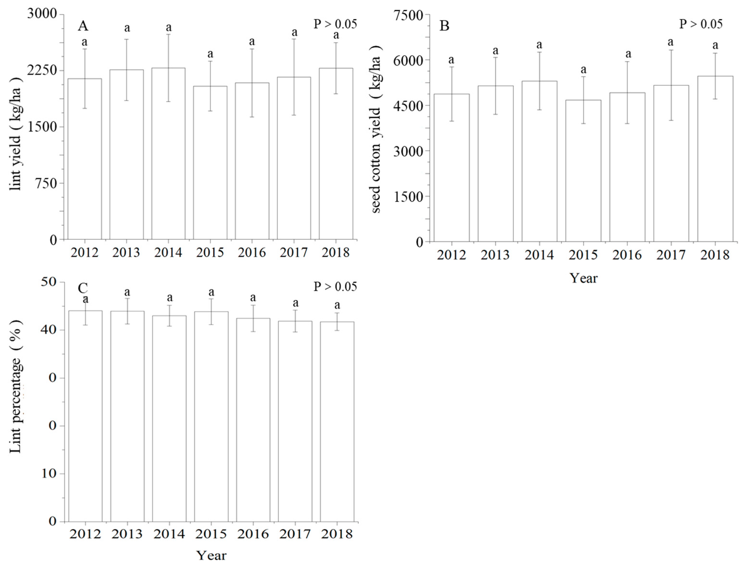
3.1. Change Pattern of Yield and Lint Percentage in the Regional Trials of Cotton Varieties from 2012 to 2018

No significant differences were observed in both lint yield and seed cotton yield from 2012 to 2018 (Figure 1). During this period, lint yield ranged from 2044.4 kg/ha to 2261.5 kg/ha, and seed cotton yield ranged from 4667.8 kg/ha to 5462.7 kg/ha. The lowest average yield occurred in 2015, while the highest seed cotton yield was recorded in 2018, and the highest lint yield was recorded in 2014. However, the patterns of lint yield and seed cotton yield did not follow the same trend. Lint percentages of cotton varieties remained stable from 2012 to 2018 (Figure 1C) and did not show significant differences between years (p < 0.05). The mean lint percentage ranged from 40.9% to 42.3%. The interannual fluctuations were primarily influenced by differences in the participating varieties and some variations in meteorological conditions.

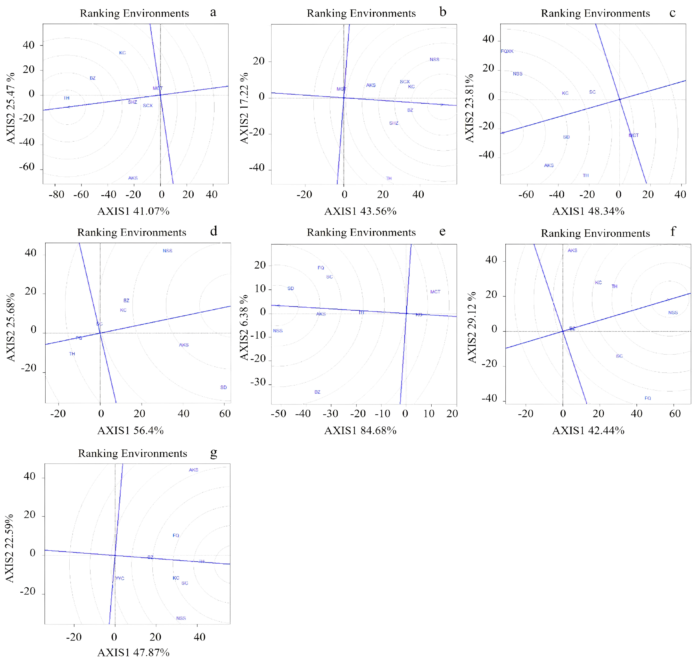
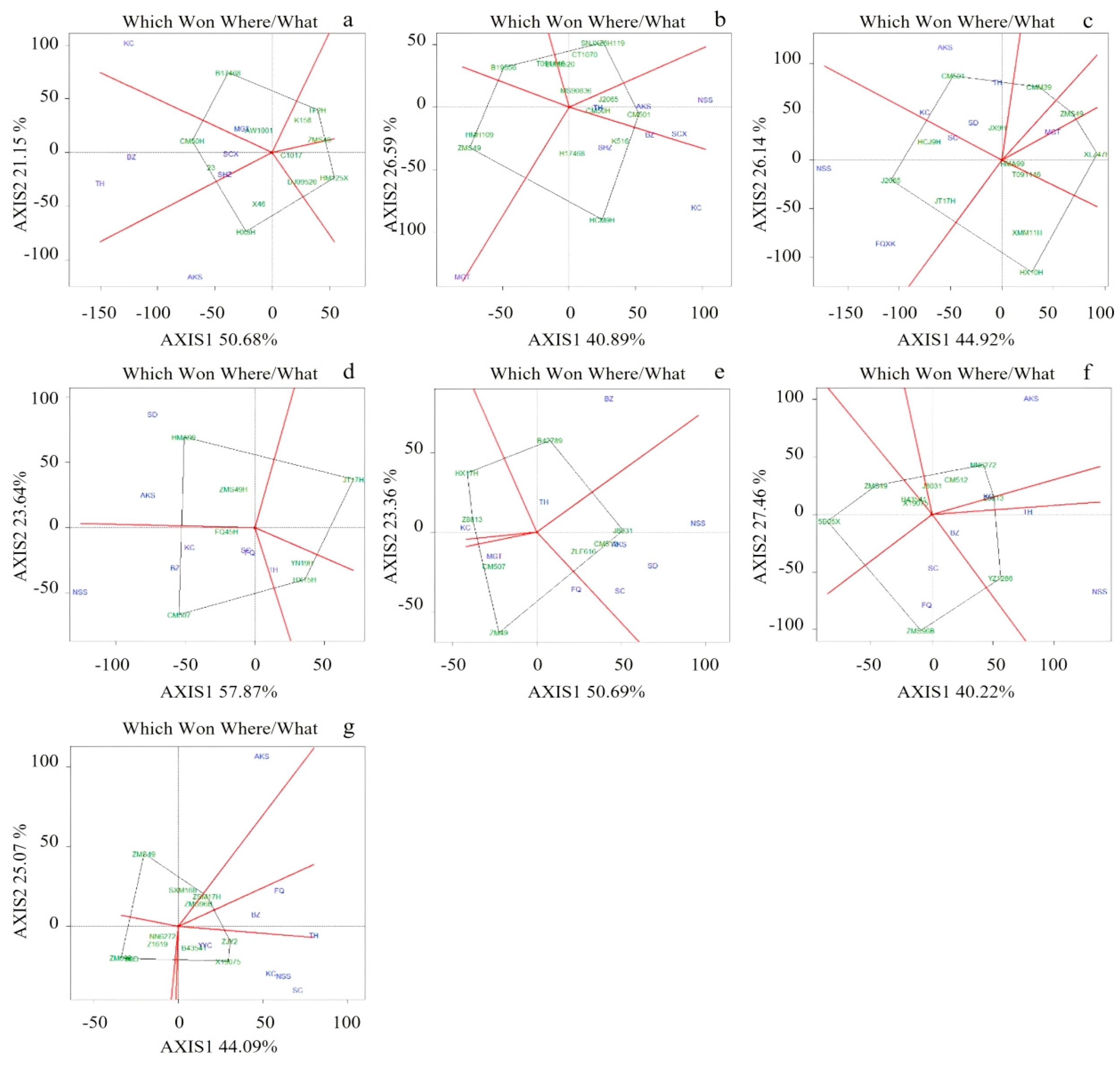
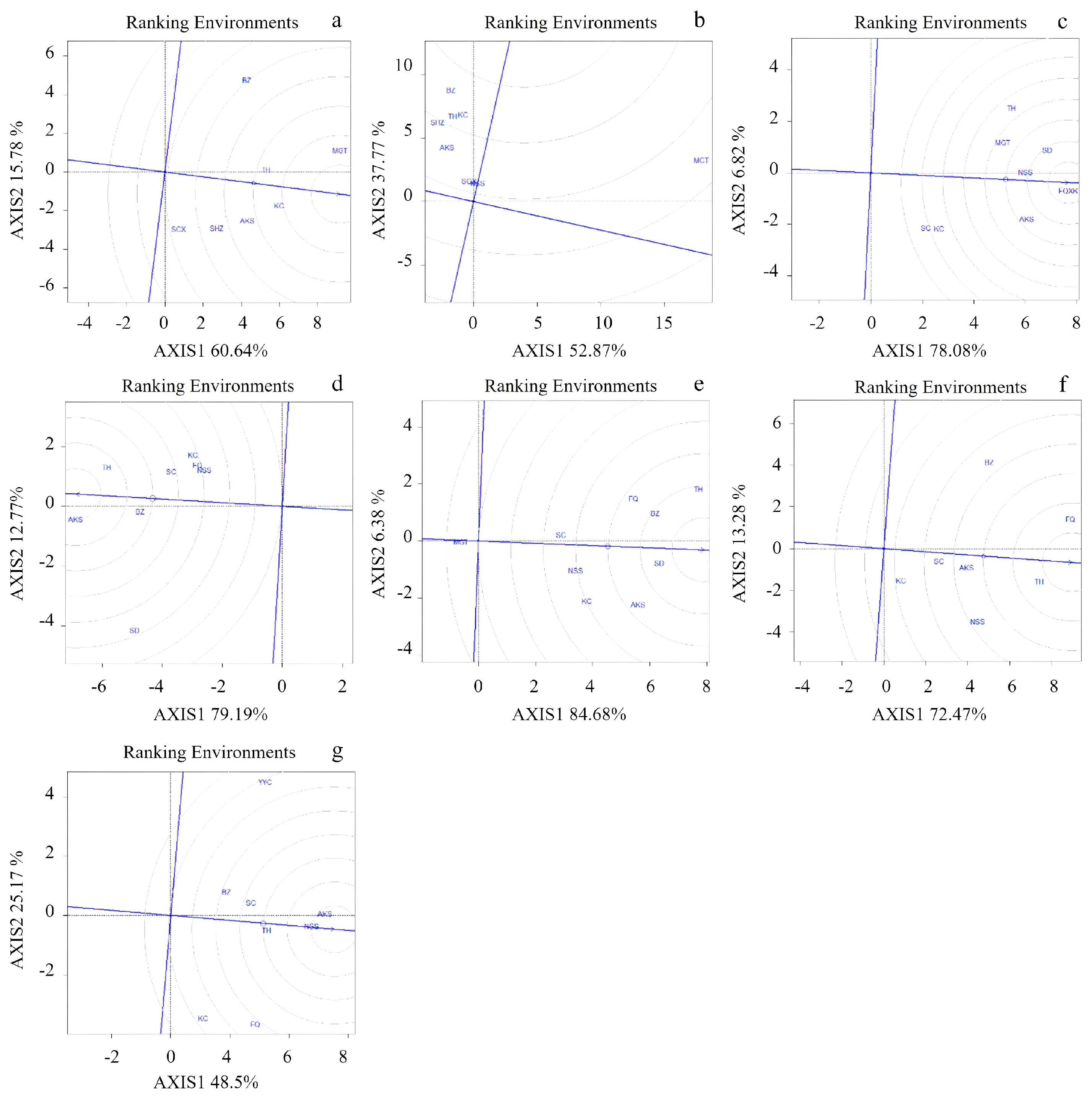
3.2. Cotton Planting Area Division Based on Yield

The cotton planting area division based on lint yield is shown in Figure 2. In 2012, the areas were divided into three sectors: AKS/SC/SHZ with HX8H as the winning genotype, TH, and BZ/KC/MGT with B17168 at the vertex. In 2013, the divisions were MGT with CM50H as the winning genotype, AKS/SC/NSS with J2065 as the winning genotype, and KC/BZ/SHZ/TH with HCM9H as the winning genotype. The 2014 division included four sectors: FQ/NSS/KC/SC with J2065 as the winning genotype, SD/AKS with HMA99 as the winning genotype, TH with JX9H as the winning genotype, and MGT with ZMS49 as the winning genotype. In 2015, three sectors were formed: NSS/BZ/KC/SC, FQ with CM507 as the winning genotype, TH with JT17H as the winning genotype, and AKS/SD with HMA99 at the vertex. The 2016 divisions included three sectors: KC with Z8813 at the vertex, MGT with ZM49 as the winning genotype, and FQ/NSS/AKS/BZ/TH/SC/FQ with J8031 as the winning genotype. In 2017, the sectors were AKS/KC with CM512 as the winning genotype, TH/NSS/SC/BZ with YZ1286 as the winning genotype, and FQ with ZMS96B as the winning genotype. And in 2018, there were four subzones: AKS/FQ with ZSM17H as the winning genotype, BZ/TH/KC/SC with ZJY2 as the winning genotype, NSS, and MGT. The sector distributions showed no obvious patterns, and the sites with the largest differentiation from 2012 to 2018 were TH, BZ, AKS, SD, NLS, and TH, respectively (Figure A1). The evaluation of zoning and site differentiation based on lint yield showed significant interannual variation.

Based on seed cotton yield, the “which-won-where/what” map (Figure 3) revealed three partitions in 2012 (MGT/KC with B17468 as the winning genotype, SC/SHZ/BZ/TH with CM50H as the winning genotype, and AKS with HX8H as the winning genotype), three partitions in 2013 (MGT, AKS/SC/NSS with HCM9H as the winning genotype, KC/BZ/SHZ/TH with CM501 as the winning genotype), and three partitions in 2014 (FQ/NSS/KC/SC with J2065 as the winning genotype, SD/AKS/ KC/TH with CM501 as the winning genotype, and MGT). In 2015, three divisions emerged: NSS/BZ/KC/SC/FQ with CM507 at the vertex, TH with HX15H at the vertex, and AKS/SD with NMA99 at the vertex. The 2016 divisions were: KC with ZMS96B at the vertex, MGT/FQ with ZM49 at the vertex, BZ/TH with B42789 at the vertex, AKS /NSS/SC /SD with J8031 at the vertex. And in 2017, the sectors were AKS/KC with NN6272 as the winning genotype, TH/BZ /NSS with YZ1286 as the winning genotype, and FQ/SC with ZMS96B at the vertex. In 2018, the subzones were: AKS, BZ/TH/FQ, and NSS/KC/SC/MGT with X15075 at the vertex.

The partitions based on seed cotton yield not only displayed large interannual differences but also varied greatly from the partitions based on lint yield. According to the results in Figure A2, the sites with the largest differentiation in seed cotton yield were TH, KC, AKS, SD, NSS, and TH. These differences in lint cotton yield in two years indicate that the relationship between seed and lint yields is not entirely consistent. The primary reason for this discrepancy is the fluctuation of the lint percentage, which refers to the changing composition of seed cotton yield.

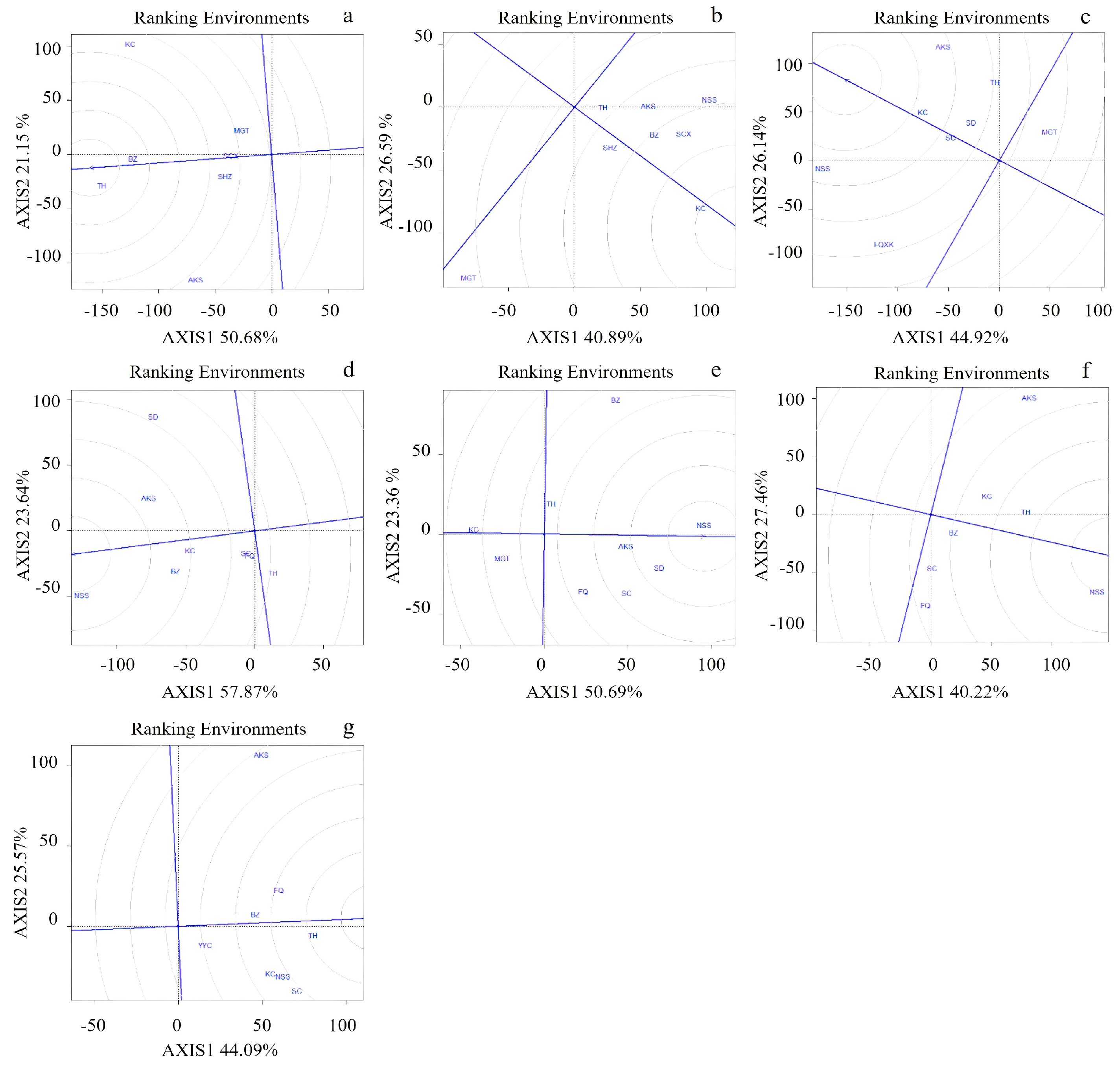
3.3. Division of Cotton Planting Areas Based on Lint Percentage

From 2012 to 2018, the sites with the highest degree of differentiation were MGT, BZ, FQ, AKS, SD, TH, and AKS. The sites with the lowest degree of differentiation were SC, SC, SC, SD, MGT, KC, and KC. The degree of differentiation in lint percentages showed some regularity; for example, the sites with the lowest degree of differentiation in the consecutive years 2012–2013 and 2017–2018 were consistent. However, there were also large fluctuations, such as the SHZ site, which had the lowest differentiation in 2012 and the highest in 2014. Considering that variety trials typically require adequate water and fertilizer, these fluctuations in differentiation are likely linked to the variation in field microclimates. Future research on variety trials should strengthen the observation of field microclimates to better understand these patterns.

The “which-won-where/what” plot of the lint percentage results from 2012 to 2018 (Figure 4) revealed the following divisions: In 2012, there were two partitions (BZ/MGT/TH with DJ09520 at the vertex, KC/AKS/SHZ/SC with HM125X as the winning genotype); in 2013, there were two partitions (MGT, SC/AKS/TH/KC/BZ/SHZ with DJ09520 as the winning genotype); in 2014, the divisions were SC/KC with J2665 as the winning genotype and AKS/FQ/NSS/FQ/SC/TH/MGT with HMA99 as the winning genotype; in 2015, the divisions were SC/TH/FQ/NSS, KC with YN19H as the winning genotype, and AKS /SD /BZ with HMA99 as the winning genotype; in 2016, the divisions were MGT with Z8813 as the winning genotype, SC/FQ/BZ/TH/SD with ZLF618 as the winning genotype, and NSS/KC/AKS; in 2017, the sectors were BZ/FQ with J8031 as the winning genotype and TH/AKS/SC/NSS with CM512 as the winning genotype; and in 2018, the divisions were KC, FQ, and TH/NSS/AKS/CS/BZ/MGT with ZSM17H as the winning genotype.

The division of planting subzones based on lint percentage also exhibited significant fluctuations. It is generally assumed that two sites with an angle greater than 90° between the connecting line and the zero point coordinates are extremely different. Based on Figure 5, it can be observed that the WS site was difficult to categorize within 90° of most sites in certain years, suggesting this site may have specific geographical characteristics related to fertility. However, the presence of interannual variability was not sufficient to stabilize the classification into distinct subzones.

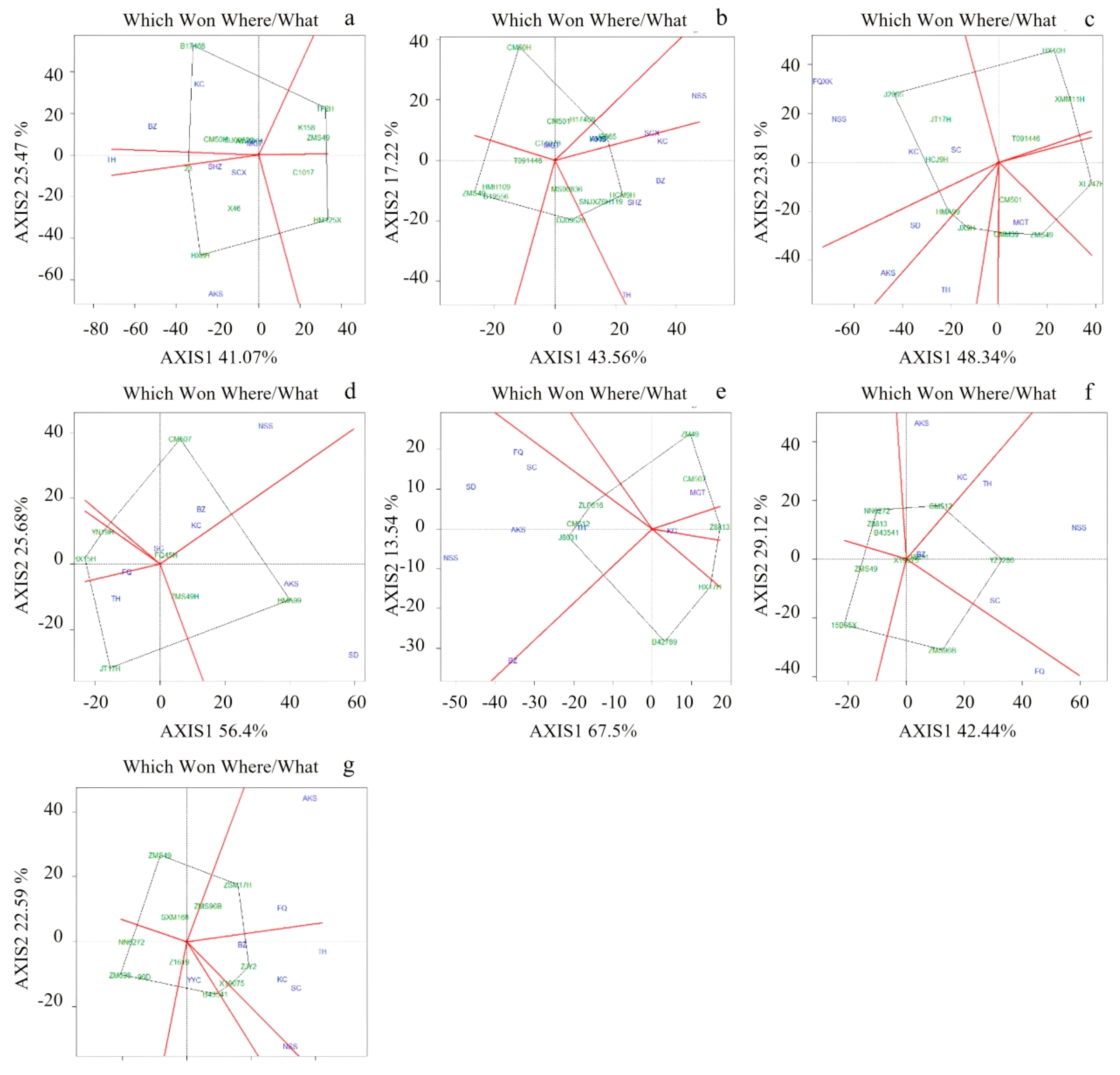
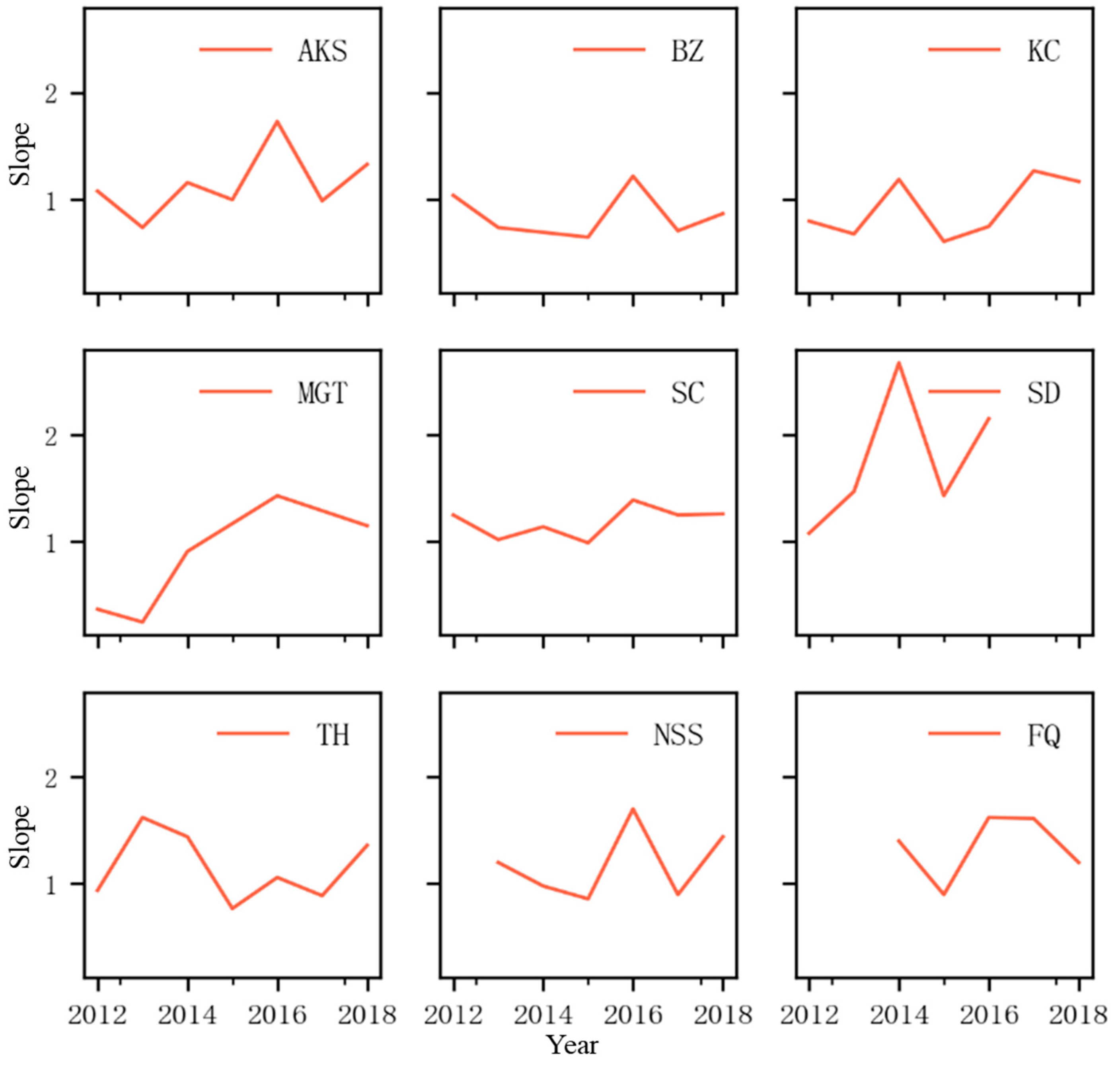
3.4. Heterozygous Growth of Seed Cotton Composition on Sites

Heterozygous growth in seed cotton composition was generalized across sites. The results of heterozygous growth calculations at each experimental site from 2012 to 2018 are shown in

Table 3. SMA analysis results of different sites from 2012 to 2018.

Year	Group	Slope	95%CI	Interc	95%CI	R2	p
2012	AKS	1.08	0.82~1.42	0.28	0.92~0.37	0.85	<0.01
	BZ	1.04	0.66~1.64	0.19	1.32~0.94	0.55	<0.01
	KC	0.8	0.56~1.14	0.34	0.33~1.01	0.73	<0.01
	MGT	0.37	0.2~0.68	1.33	0.8~1.87	0.12	0.27
	SC	1.25	0.86~1.83	0.77	−1.88~0.35	0.7	<0.01
	SHZ	1.08	0.66~1.78	−0.23	−1.44~0.98	0.46	<0.05
	TH	0.94	0.66~1.34	0.04	−0.75~0.84	0.74	<0.01
2013	AKS	0.74	0.5~1.09	0.46	−0.19~1.11	0.6	<0.01
	BZ	0.74	0.43~1.27	0.53	−0.42~1.48	0.17	0.15
	KC	0.68	0.45~1.02	0.63	−0.03~1.29	0.54	<0.01
	MGT	0.25	0.14~0.45	1.63	1.28~1.99	0.01	0.8
	NSS	1.2	0.87~1.67	−0.59	−1.55~0.37	0.72	<0.01
	SC	1.02	0.8~1.31	−0.17	−0.75~0.4	0.84	<0.01
	SHZ	1.47	0.92~2.33	−1.11	−2.63~0.42	0.42	<0.01
	TH	1.62	0.93~2.81	−1.58	−3.78~0.62	0.15	0.17
2014	AKS	1.16	0.81~1.65	−0.51	−1.46~0.44	0.74	<0.01
	FQ	1.4	0.9~2.18	−1.05	−2.56~0.47	0.57	<0.01
	KC	1.19	0.88~1.62	−0.58	−1.42~0.27	0.8	<0.01
	MGT	0.91	0.53~1.55	0.13	−1.08~1.34	0.36	<0.05
	NSS	0.98	0.64~1.49	−0.09	−1.1~0.93	0.62	<0.01
	SC	1.14	0.83~1.58	−0.45	−1.3~0.39	0.78	<0.01
	SD	2.67	1.61~4.42	−3.82	−6.94~−0.7	0.45	<0.05
	TH	1.44	1~2.07	−1.1	−2.3~0.1	0.72	<0.01
2015	AKS	1	0.45~2.23	−0.14	−2.1~1.82	0.4	0.13
	BZ	0.65	0.37~1.14	0.7	−0.14~1.55	0.74	<0.01
	FQ	0.9	0.36~2.28	0.12	−2.08~2.32	0.14	0.41
	KC	0.61	0.32~1.16	0.79	−0.13~1.71	0.65	<0.05
	NSS	0.86	0.61~1.21	0.2	−0.5~0.9	0.91	<0.01
	SC	0.99	0.39~2.48	−0.12	−2.44~2.19	0.15	0.39
	SD	1.43	0.9~2.3	−1	−2.49~0.5	0.82	<0.01
	TH	0.77	0.3~1.96	0.41	−1.52~2.34	0.11	0.47
2016	AKS	1.73	0.8~3.75	−1.82	−5.15~1.5	0.27	0.19
	BZ	1.22	0.64~2.33	−0.62	−2.56~1.31	0.52	<0.05
	FQ	1.62	0.68~3.86	−1.58	−5.39~2.22	0.03	0.67
	KC	0.75	0.37~1.5	0.45	−0.85~1.76	0.44	0.08
	MGT	1.43	0.95~2.15	−1.07	−2.42~0.28	0.82	<0.01
	NSS	1.7	1.2~2.4	−1.84	−3.27~−0.42	0.88	<0.01
	SC	1.39	0.9~2.16	−1.06	−2.48~0.36	0.8	<0.01
	SD	2.15	1.32~3.5	−2.59	−4.93~−0.24	0.74	<0.01
	TH	1.06	0.45~2.51	−0.21	−2.38~1.97	0.04	0.62
2017	AKS	0.99	0.75~1.3	−0.14	−0.73~0.45	0.88	<0.01
	BZ	0.71	0.35~1.45	0.53	−0.69~1.75	0.09	0.39
	FQ	1.61	0.78~3.29	−1.58	−4.55~1.38	0.08	0.43
	KC	1.27	0.9~1.79	−0.74	−1.75~0.27	0.81	<0.01
	NSS	0.9	0.56~1.45	0.11	−0.97~1.19	0.63	<0.01
	SC	1.25	0.93~1.66	−0.72	−1.54~0.11	0.87	<0.01
	TH	0.89	0.47~1.7	0.11	−1.34~1.56	0.29	0.11
2018	AKS	1.33	0.8~2.21	−0.95	−2.63~0.73	0.5	<0.05
	BZ	0.87	0.57~1.33	0.16	−0.7~1.01	0.67	<0.01
	FQ	1.2	0.73~1.96	−0.59	−1.98~0.79	0.54	<0.01
	KC	1.17	0.69~1.97	−0.54	−2.05~0.97	0.47	<0.05
	NSS	1.44	0.82~2.52	−1.2	−3.22~0.82	0.39	<0.05
	SC	1.26	0.98~1.63	−0.76	−1.5~−0.03	0.88	<0.01
	TH	1.36	0.88~2.12	−0.98	−2.44~0.48	0.64	<0.01
	MGT	1.15	0.6~2.2	−0.48	−2.33~1.38	0.15	0.23

Note: CI: confidence interval; R²: determination coefficient; p < 0.05: significant; p < 0.01: extremely significant.

. The slope represents the linear trend in the results of the SMA (Weighted Average Analysis) for different locations from 2012 to 2018. It reflects the rate of change over time for certain variables (such as yield, quality, etc.) across these years. A larger slope value indicates a more significant change in the variable. A positive slope suggests that the variable increases over time, while a negative slope indicates a decrease over time. Significant differences were found at most sites, except for MGT in 2012. The slopes ranged from 0.5 to 1.1, and all were significant except for BZ, TH, and MGT in 2013, where slopes ranged from 0.7 to 4.5. In 2014, all sites reached significance with slopes ranging from 0.96 to 2.7. For 2015, sites such as AKS, FQ, SC, and TH did not reach significance, and the slopes were between 1.6 and 1.5. In 2016, AKS, FQ, and TH did not reach significance, with slopes between 0.5 and 2.6. In 2017, BZ and FQ did not reach significance, with slopes between 0.9 and 1.3. In 2018, MGT did not reach significance, and slopes ranged from 0.8 to 1.5. There were significant site differences in heterozygous growth across years.

3.5. Interannual Variation in Seed Cotton Composition of Heterozygous Growth

Slope is the primary indicator of heterozygous growth. During the 2012–2018 trials (Figure 6), the year with the lowest slope was 2014/2015, and the year with the highest slope was 2016/2017, with more obvious interannual variations at each site. TH exhibited the greatest fluctuations, ranging from 0.3 to 2.4. BZ and SC showed relatively stable heterozygous distributions (ranging from 0.6 to 1.2). AKS (0.6–1.8), FQ (0.6–1.8), KC (0.6–1.5), and SD (0.6–1.5) displayed some degree of interannual variability. Fluctuations ranged from less than 1 to greater than 1 across all nine sites, indicating that all sites experienced both positive and reverse correlations in the anisotropic velocity distribution in different years. The significance of these variations was either significant or highly significant in both years with extreme values.

4. Discussion

Lint yield is the final output of cotton cultivation, but in practice, agricultural laborers harvest seed cotton, which is purchased at ginning mills for processing into lint [33]. This process is part of the industrial sector’s scope of research. Consequently, the ratio of lint to seed cotton remains the most intuitive indicator for assessing cotton quality and determining its purchase price [34].

From 2012 to 2018, the regional trials of cotton varieties in the Northwest Inland Cotton Region did not show significant differences in seed cotton yield. The average seed cotton yield slightly declined over this period, indicating that cotton breeding has entered a relatively stable phase with respect to yield indices. It has become more difficult to increase cotton yield through varietal improvement compared to the previous century. As a result, regional trials now emphasize the regional adaptability of varieties. Similarly, there were no significant changes in lint yield from 2012 to 2018, with a slight decline observed on average, marking a bottleneck in cotton yield improvements. Therefore, the focus of cotton regional variety trials should now shift toward enhancing the regional adaptability of varieties.

Lint percentage is a key indicator of cotton yield composition and a critical determinant of seed cotton quality [35]. In practice, cotton farmers sell seed cotton to ginning mills, where it is de-seeded and sold as lint. Thus, the lint percentage is an important factor influencing the purchase price for both ginning mills and cotton farmers. The results of studies in different regions may vary due to the impact of varieties or local environments. For example, a study in Argentina found that lint percentage was primarily influenced by the genotype of cotton varieties, with little effect from environmental factors [36]. However, differences in cotton varieties used at various agro-gas stations or between years were not consistent, making it difficult to fully attribute the changes in lint percentage to environmental factors alone.

This study systematically summarized the performance of lint percentage in regional cotton variety trials from 2012 to 2018. It was found that no clear pattern emerged in terms of lint percentage based on sites or varieties, and fluctuations in lint percentage could not be linked to a consistent trend across the time series. Interannual fluctuations in lint percentage were extremely large, with sites showing both high and low differentiation across years. Some sites even exhibited drastic changes, being the most differentiated in one year and the least differentiated in another [37]. This variability highlights that cotton production in the Northwest Inland Cotton Region of China is highly sensitive to the combined effects of varieties and sites, and the premature promotion of certain varieties could result in a decline in cotton quality [38]. Therefore, it is crucial to evaluate whether new varieties are suitable for promotion through extended demonstration periods.

The heterosis growth patterns of seed cotton and lint yield also support this phenomenon. The generally low heterosis growth index (slope) observed in 2015 may be related to the specific varieties tested, while the site-specific fluctuations in the heterosis growth index observed in 2016 and 2017 are likely due to environmental factors.

Previous research has often assigned higher ratings to sites with greater varietal differences within the same region, as such sites are favorable for selecting and breeding high-yielding varieties [39,40]. However, sites with higher varietal differences tend to also exhibit larger yield and quality differences, particularly in regions like MGT, BZ, FQ, AKS, SD, and TH, where lint percentage differentiation varied significantly over the years. These sites should be carefully considered during varietal promotion to avoid potential quality declines, especially if some varieties have excessively high seed weights, leading to low purchase prices. In contrast, sites such as SC and KC, where lint percentage differentiation was minimal, showed more stable performance over the years. Therefore, promoting multiple varieties in these areas is less likely to result in large fluctuations in lint percentage. This conclusion is further supported by the analysis of the allometry distribution index across the sites.

5. Conclusions

Based on the 2012–2018 regional trials in the Northwest Inland Cotton Region, and utilizing the GGE biplot diagrams to analyze regional differences in variety trials over several years, we found that seed cotton yield, lint yield, and lint percentage exhibited significant interannual fluctuation. These fluctuations were especially notable between the best- and worst-performing sites, although regional partitioning based on the average values can still be performed. However, the yield and quality differences caused by varietal variations at specific sites should be emphasized in actual cotton production.

The heterosis growth model was applied to assess heterosis growth patterns of lint and seed yields across different sites from 2012 to 2018. The results indicated that most sites exhibited highly significant or significant heterosis growth, with notable site differences. Lint yield and seed weight at the site scale generally conformed to the allometry distribution model, showing large interannual fluctuations in the allometry distribution index at sites such as Shihezi, Tahe, and Aksu, and smaller fluctuations at sites like Kuqa and Shache. These findings align with the results from the GGE model analysis of lint percentage differentiation, demonstrating that the allometry distribution index can be used to assess interannual variations in varietal differences within a site.

The substantial interannual fluctuations in lint percentage and yield outcomes may be related to the varieties selected each year, and environmental factors play a crucial role in these variations. Given the unique microclimates of the oases in the Northwest Inland Cotton Region, it is recommended that future variety trials incorporate more comprehensive microclimate observations to better understand the environmental influences on cotton production.

References

1. Markinos, A.T.; Gemtos, T.A.; Pateras, D.; Toulios, L.; Zerva, G.; Papaeconomou, M. The influence of cotton variety in the calibration factor of a cotton yield monitor. Oper. Res. Int. J. 2005, 5, 165–176. [Google Scholar] [CrossRef]
2. Desrochers, P.; Szurmak, J. Long Distance Trade, Locational Dynamics and By-Product Development: Insights from the History of the American Cottonseed Industry. Sustainability 2017, 9, 579. [Google Scholar] [CrossRef]
3. Stewart, S. A Community Crop: Cotton, Science, and Extension in Interwar Shandong, 1918–1937. Twent.-Century China 2021, 46, 199–219. [Google Scholar] [CrossRef]
4. Zhu, Y.; Zheng, B.; Luo, Q.; Jiao, W.; Yang, Y. Uncovering the Drivers and Regional Variability of Cotton Yield in China. Agriculture 2023, 13, 2132. [Google Scholar] [CrossRef]
5. Dai, J.; Dong, H. Intensive cotton farming technologies in China: Achievements, challenges and countermeasures. Field Crops Res. 2014, 155, 99–110. [Google Scholar] [CrossRef]
6. Feng, L.; Dai, J.; Tian, L.; Zhang, H.; Li, W.; Dong, H. Review of the technology for high-yielding and efficient cotton cultivation in the northwest inland cotton-growing region of China. Field Crops Res. 2017, 208, 18–26. [Google Scholar] [CrossRef]
7. Chen, W.; Hou, Z.; Wu, L.; Liang, Y.; Wei, C. Effects of salinity and nitrogen on cotton growth in arid environment. Plant Soil. 2010, 326, 61–73. [Google Scholar] [CrossRef]
8. Vitale, G.S.; Aurelio, S.; Silvia, Z.; Teresa, T.; Carmelo, S.; Gaetano, P.; Sara, L.; Umberto, A.; Paolo, G. Agronomic Strategies for Sustainable Cotton Production: A Systematic Literature Review. Agriculture 2024, 14, 1597. [Google Scholar] [CrossRef]
9. Khan, A.; Tan, D.K.Y.; Munsif, F.; Afridi, M.Z.; Shah, F.; Wei, F.; Fahad, S.; Zhou, R. Nitrogen nutrition in cotton and control strategies for greenhouse gas emissions: A review. Environ. Sci. Pollut. Res. 2017, 24, 23471–23487. [Google Scholar] [CrossRef]
10. Macdonald, B.C.T.; Chang, Y.F.; Nadelko, A.; Tuomi, S.; Glover, M. Tracking fertiliser and soil nitrogen in irrigated cotton: Uptake, losses and the soil N stock. Soil. Res. 2016, 55, 264–272. [Google Scholar] [CrossRef]
11. Tao, R.; Wakelin, S.A.; Liang, Y.; Chu, G. Organic Fertilization Enhances Cotton Productivity, Nitrogen Use Efficiency, and Soil Nitrogen Fertility under Drip Irrigated Field. Agron. J. 2017, 109, 2889–2897. [Google Scholar] [CrossRef]
12. Boulal, H.; Gómez-Macpherson, H.; Villalobos, F.J. Permanent bed planting in irrigated Mediterranean conditions: Short-term effects on soil quality, crop yield and water use efficiency. Field Crops Res. 2012, 130, 120–127. [Google Scholar] [CrossRef]
13. Ma, Z.B.; Gong, Y.F.; Han, M.; Li, L.L.; Zhu, W. The influence of different soil textures on the spatiotemporal distribution and yield of cotton boll formation. J. Henan Agric. Univ. 2011, 45, 497–501. [Google Scholar]
14. Nouri, A.; Lee, J.; Yin, X.; Tyler, D.D.; Saxton, A.M. Thirty-four years of no-tillage and cover crops improve soil quality and increase cotton yield in Alfisols, Southeastern USA. Geoderma 2019, 337, 998–1008. [Google Scholar] [CrossRef]
15. Moreno, P.M.; Sproul, E.; Quinn, J.C. Economic and environmental sustainability assessment of guayule bagasse to fuel pathways. Ind. Crops Prod. 2022, 178, 114644. [Google Scholar] [CrossRef]
16. Shojaei, S.H.; Mostafavi, K.; Bihamta, M.R.; Omrani, A.; Mousavi, S.M.N.; Illés, Á.; Bojtor, C.; Nagy, J. Stability on Maize Hybrids Based on GGE Biplot Graphical Technique. Agronomy 2022, 12, 394. [Google Scholar] [CrossRef]
17. Lee, S.Y.; Lee, H.S.; Lee, C.M.; Ha, S.K.; Park, H.; Lee, S.; Kwon, Y.; Jeung, J.U.; Mo, Y. Multi-Environment Trials and Stability Analysis for Yield-Related Traits of Commercial Rice Cultivars. Agriculture 2023, 13, 256. [Google Scholar] [CrossRef]
18. Malosetti, M.; Ribaut, J.-M.; van Eeuwijk, F.A. The statistical analysis of multi-environment data: Modeling genotype-by-environment interaction and its genetic basis. Front. Physiol. 2013, 4, 44. [Google Scholar] [CrossRef]
19. Wu, J.; Wang, Y.; Xiang, L.; Gu, Y.; Yan, Y.; Li, L.; Tian, X.; Jing, W.; Wang, X. Machine learning model to predict the efficacy of antiseizure medications in patients with familial genetic generalized epilepsy. Epilepsy Res. 2022, 181, 106888. [Google Scholar] [CrossRef]
20. Beninde, J.; Veith, M.; Hochkirch, A. Biodiversity in cities needs space: A meta-analysis of factors determining intra-urban biodiversity variation. Ecol. Lett. 2015, 18, 581–592. [Google Scholar] [CrossRef]
21. Cassman, K.G. Ecological intensification of cereal production systems: Yield potential, soil quality, and precision agriculture. Proc. Natl. Acad. Sci. USA 1999, 96, 5952–5959. [Google Scholar] [CrossRef] [PubMed]
22. Isaacs, K.; Weltzien, E.; Some, H.; Diallo, A.; Diallo, B.; Sidibé, M.; vom Brocke, K.; Samake, B.; Nebié, B.; Rattunde, F.W. Increasing sorghum yields for smallholder farmers in Mali: The evolution towards a context-driven, on-farm, gender-responsive sorghum breeding program. Front. Sustain. Food Syst. 2024, 8, 1334385. [Google Scholar] [CrossRef]
23. Lin, B.B. Resilience in Agriculture through Crop Diversification: Adaptive Management for Environmental Change. BioScience 2011, 61, 183–193. [Google Scholar] [CrossRef]
24. Yan, W.K. GGEbiplot—A Windows Application for Graphical Analysis of Multienvironment Trial Data and Other Types of Two-Way Data. Agron. J. 2001, 93, 1111–1118. [Google Scholar] [CrossRef]
25. Xu, N.Y.; Zhang, G.W.; Li, J.; Zhou, Z. Environmental evaluation of cotton regional test in Yangtze River Basin based on GGE biplot and fiber length selection. Resour. Environ. Yangtze Basin 2013, 22, 735–741. [Google Scholar] [CrossRef]
26. Tang, S.R.; Xu, N.Y.; Yang, W.H.; Wei, S.; Zhou, Z. Is based on the analysis of the GGE northwest inland cotton fiber quality ecological division. J. Chin. Ecol. Agric. 2016, 24, 1674–1682. [Google Scholar] [CrossRef]
27. Daemo, B.B.; Zeleke, A. Application of AMMI and GGE biplot for genotype by environment interaction and yield stability analysis in potato genotypes grown in Dawuro zone, Ethiopia. J. Agric. Food Res. 2024, 18, 101287. [Google Scholar] [CrossRef]
28. Liu, Y.; Zhao, X.; Liu, W.; Feng, B.; Lv, W.; Zhang, Z.; Yang, X.; Dong, Q. Plant biomass partitioning in alpine meadows under different herbivores as influenced by soil bulk density and available nutrients. Catena 2024, 240, 108017. [Google Scholar] [CrossRef]
29. Matloob, A.; Aslam, F.; Rehman, H.U.; Khaliq, A.; Ahmad, S.; Yasmeen, A.; Hussain, N. Cotton-Based Cropping Systems and Their Impacts on Production. In Cotton Production and Uses: Agronomy, Crop Protection, and Postharvest Technologies; Ahmad, S., Hasanuzzaman, M., Eds.; Springer: Singapore, 2020; pp. 283–310. [Google Scholar] [CrossRef]
30. Wang, C.X.; Yuan, W.M.; Liu, J.J.; Xie, X.Y.; Ma, Q.; Jiu, J.S.; Chen, Y.Y.; Wang, N.; Feng, K.Y.; Su, J.J. Comprehensive evaluation and breeding evolution of early-maturing landrace cotton varieties in inland Northwest China. Chin. Agric. Sci. 2023, 56, 1–21. [Google Scholar]
31. Thorp, K.R.; Ale, S.; Bange, M.P.; Barnes, E.M.; Hoogenboom, G.; Lascano, R.J.; McCarthy, A.C.; Nair, S.; Paz, J.O.; Rajan, N.; et al. Development and application of process-based simulation models for cotton production: A review of past, present, and future directions. J. Cotton Sci. 2014, 18, 10–47. [Google Scholar] [CrossRef]
32. Westgeest, A.J.; Vasseur, F.; Enquist, B.J.; Milla, R.; Gómez-Fernández, A.; Pot, D.; Vile, D.; Violle, C. An allometry perspective on crops. New Phytol. 2024, 244, 1223–1237. [Google Scholar] [CrossRef]
33. Hardin, R.G.; Barnes, E.M.; Delhom, C.D.; Wanjura, J.D.; Ward, J.K. Internet of things: Cotton harvesting and processing. Comput. Electron. Agric. 2022, 202, 107294. [Google Scholar] [CrossRef]
34. Sun, Q.; Chen, S.; Sun, L.; Qiao, C.; Li, X.; Wang, L. Calculation and evaluation of cotton lint carbon footprint based on different cotton straw treatment methods: A case study of Northwest China. J. Clean. Prod. 2024, 484, 144374. [Google Scholar] [CrossRef]
35. Tlatlaa, J.S.; Tryphone, G.M.; Nassary, E.K. Unexplored agronomic, socioeconomic and policy domains for sustainable cotton production on small landholdings: A systematic review. Front. Agron. 2023, 5, 1281043. [Google Scholar] [CrossRef]
36. Scarpin, G.J.; Dileo, P.N.; Winkler, H.M.; Cereijo, A.E.; Lorenzini, F.G.; Roeschlin, R.A.; Muchut, R.J.; Acuña, C.; Paytas, M. Genetic progress in cotton lint and yield components in Argentina. Field Crops Res. 2022, 275, 108322. [Google Scholar] [CrossRef]
37. Zhang, Q.H.; He, W.Z.; Pei, M.Y. Analysis of yield and related traits of spring cotton varieties approved by the state in the Yellow River Basin from 2011 to 2020. China Cotton 2023, 50, 17–21. [Google Scholar] [CrossRef]
38. Mao, S.C.; Cheng, S.X.; Ma, X.Y.; Wei, S.J.; Tang, S.R.; Wang, W.K.; Wang, Z.B. Quality Changes of Main Cotton Varieties in Xinjiang from 2018 to 2020 and Suggestions for Selection and Promotion of High Quality Cotton Varieties. China Cotton 2021, 48, 1–7. [Google Scholar]
39. Benaragama, D.; Rossnagel, B.G.; Shirtliffe, S.J. Breeding for Competitive and High-Yielding Crop Cultivars. Crop Sci. 2014, 54, 1015–1025. [Google Scholar] [CrossRef]
40. Joshi, K.D.; Musa, A.M.; Johansen, C.; Gyawali, S.; Harris, D.; Witcombe, J.R. Highly client-oriented breeding, using local preferences and selection, produces widely adapted rice varieties. Field Crops Res. 2007, 100, 107–116. [Google Scholar] [CrossRef]
Figure 1. Regional trial yield of cotton varieties in 2012–2018. (A) The lint yield of cotton, (B) the seed cotton yield of cotton, and (C) the lint percentage of cotton. p represents significance. Different lowercase letters indicate significant differences between different years (p > 0.05 is not significant).
Agronomy 15 00989 g001
Figure 2. Which won what/where chart of lint yield in the Northwest Inland Cotton Region from 2012 to 2018: (a) 2012, (b) 2013, (c) 2014, (d) 2015, (e) 2016, (f) 2017, (g) 2018.
Agronomy 15 00989 g002
Figure 3. Which won what/where for the yield of seed cotton in the Northwest Inland Cotton Region from 2012 to 2018: (a) 2012, (b) 2013, (c) 2014, (d) 2015, (e) 2016, (f) 2017, (g) 2018.
Agronomy 15 00989 g003
Figure 4. Which won what/where for the lint percentage in the Northwest Inland Cotton Region from 2012 to 2018: (a) 2012, (b) 2013, (c) 2014, (d) 2015, (e) 2016, (f) 2017, (g) 2018.
Agronomy 15 00989 g004
Figure 5. Ranking environments for lint percentage in the Northwest Inland Cotton Region from 2012 to 2018: (a) 2012, (b) 2013, (c) 2014, (d) 2015, (e) 2016, (f) 2017, (g) 2018.
Agronomy 15 00989 g005
Figure 6. Interannual variation of slope in Northwest Inland Cotton Region from 2012 to 2018. The vertical slope represents the degree of skewness and the horizontal coordinates represent different planting years. AKS represents Aksu; BZ represents Bazhou; KC represents Kuche; MGT represents Maigaiti; SC represents Shache; SD represents Shihezi University; TH represents Tahe; NSS represents Nongliushi; FQ represents Fuquan.
Agronomy 15 00989 g006