Abstract
In modern agricultural production, accurately estimating the leaf water content (LWC) of Korla fragrant pear is crucial for achieving scientific irrigation and ensuring fruit quality. However, constructing accurate and effective LWC prediction models remains challenging due to limitations in sample selection, spectral feature analysis, and model applicability. To address these issues, this study was conducted to systematically optimize the process. During sample collection, a random split method was employed to divide the dataset into modeling and testing sets at a ratio of 75%:25%. This approach ensures computational efficiency, avoids data leakage, and balances training and evaluation needs, particularly for small- to medium-sized datasets. Specifically, in stage S1, 352 samples were allocated to the modeling set and 108 to the testing set, while in stage S2, 137 and 58 samples were assigned, respectively. The analysis revealed slight differences in LWC distribution and standard deviation between the modeling and testing sets, validating the scientific rigor of dataset division. For instance, the LWC distribution in the S1 modeling set ranged from 4.88% to 83.45%, with a standard deviation of 11.33%. The spectral acquisition process within the range of 4000 cm−1 to 10,000 cm−1 exhibited complex absorbance variation trends, showing distinct characteristics across different intervals. Preprocessing techniques such as SG convolution smoothing, MSC, and SNV significantly reduced the absorbance variability and enhanced spectral features. Notably, the selection of LWC feature bands differed markedly between stages S1 and S2. For example, in S1, SNV-SPA (successive projections algorithm) feature bands were concentrated around 5000 cm−1, 6000 cm−1, and 7000 cm−1, whereas their positions shifted significantly in S2, reflecting the growth dynamics of the Korla fragrant pear. During the model-building phase, various algorithms, including Random Forest Regression (RFR), Backpropagation Neural Network (BP), and Support Vector Regression (SVR), were compared. Under different feature selections, the RFR model demonstrated strong predictive ability with determination coefficients (R2) exceeding 0.75 and root mean square errors (RMSE) below 0.7%. Specifically, the SNV-CARS-BP model achieved an R2 of 0.81594 in S1, while the SNV-SPA-RFR model reached an R2 of 0.817756 in S2, with relative deviations between the predicted and actual values of less than 5%. These results provide robust support for the precise LWC monitoring of Korla fragrant pear and offer valuable insights for subsequent research.
1. Introduction
In the context of the close interconnection between modern agricultural scientific research and production practices, the precise measurement and in-depth analysis of crop physiological characteristic parameters have become essential for advancing agriculture towards refined and scientifically informed management, thereby ensuring the high quality and yield of crops [1,2].
As a fruit variety distinguished by its unique characteristics and significant economic value in China, the Korla Xiangli enjoys considerable popularity in both domestic and international markets. The key physiological index of leaf water content (LWC) serves as a barometer for crop growth, providing direct and comprehensive insights into growth trends, water metabolism levels, and the overall health status of plants. Understanding the mechanisms underlying the growth and development of Korla fragrant pear is crucial for optimizing planting management strategies.
In recent years, spectral analysis technology has demonstrated significant potential in the detection of crop physiological parameters, owing to its advantages of non-destructive testing, rapid data acquisition, and the ability to reveal the chemical structural characteristics of substances [3,4,5]. Building on this foundation, in the present study, spectral data were collected from Korla fragrant pear leaves, characteristic information related to LWC was accurately extracted, and a reliable and efficient predictive model was developed.
Sample collection serves as the foundation of this research, with the quality of the dataset directly influencing the reliability and generalization capability of the model [6]. Korla fragrant pear exhibits significant variations in physiological characteristics and water requirements across different growth stages [7], particularly during the late fruit expansion phase (S1) and the early maturity phase (S2). During the S1 stage, the fruit undergoes rapid expansion, accompanied by active cell division and material accumulation, which heavily depend on nutrients synthesized through leaf photosynthesis and an adequate water supply [8]. LWC plays a pivotal role in regulating photosynthetic efficiency, nutrient transport, and overall plant metabolism, ultimately determining the quality of fruit expansion [9,10,11]. As the fruit transitions into the S2 stage, key quality attributes such as sweetness, color, and texture begin to stabilize [12].
However, existing research predominantly focuses on isolated growth stages, lacking a comprehensive exploration of the distinct key growth phases of Korla fragrant pear, such as the fruit enlargement and maturity stages. Furthermore, studies on the spectral detection of LWC in Korla fragrant pear remain limited, and a cohesive theoretical framework and technical methodology have yet to be established.
Given the unique characteristics of the S1 and S2 stages, this study employs a scientifically sound random splitting method to partition the dataset. This approach ensures an accurate capture of the data distribution patterns of pears across different growth phases while minimizing potential biases [13]. Specifically, 75% of the samples are allocated for model development, and the remaining 25% are reserved for testing model performance. Additionally, the sample size is carefully selected based on the distinct growth traits of the S1 and S2 stages, ensuring that the dataset comprehensively reflects the actual conditions of each phase. This meticulous approach lays a robust data foundation for subsequent research.
The spectral data obtained within the 4000–10,000 cm−1 range exhibit complex trends, with significant fluctuations in absorbance values. While these data contain rich spectral feature information, they are also plagued by interference factors such as baseline shifts and noise, which impede the precise extraction of LWC-related features [14,15,16]. Despite these challenges, existing research predominantly relies on a single preprocessing method, lacking a thorough exploration and optimization of the combined effects of multiple preprocessing techniques.
Spectral preprocessing plays a pivotal role in addressing the complexities of spectral data. The SG (Savitzky–Golay) convolution smoothing method enhances the smoothness of spectral curves, providing a stable foundation for subsequent analysis [17]. Meanwhile, MSC (Multiplicative Scatter Correction) and SNV (Standard Normal Variate) techniques effectively eliminate baseline shifts and background interference, thereby enhancing spectral features and creating optimal conditions for identifying characteristic wavelengths [18]. On the other hand, FD (first derivative) and SD (second derivative) transformations excel at highlighting subtle spectral changes, such as the positions of reflection peaks and valleys. However, these methods are prone to amplifying noise, potentially introducing glitch phenomena [19]. Given these considerations, the judicious selection and combination of preprocessing methods are crucial for optimizing spectral data quality, laying a solid groundwork for subsequent research.
Feature band selection is a critical factor influencing the overall performance of a model. However, research on the extraction of characteristic wavelengths for Korla fragrant pear LWC remains limited, and the variations in these wavelengths across different growth stages have yet to be fully elucidated. Notably, the LWC characteristic bands of Korla fragrant pear exhibit significant differences between the S1 and S2 periods, reflecting dynamic changes in leaf physiological traits, chemical composition, and spectral interactions. By precisely identifying these characteristic bands, researchers can optimize spectral models to better align with the actual growth patterns of pears, thereby enhancing the accuracy and reliability of leaf water content predictions. For instance, Ye et al. [20] successfully employed a hyperspectral imaging system (866.4–1701.0 nm) combined with the CARS (Competitive Adaptive Reweighted Sampling) algorithm to extract spectral features, achieving an impressive 97.92% accuracy in shrimp freshness recognition using an ELM (Extreme Learning Machine) model. Tang et al. [21] utilized hyperspectral technology to detect soil nitrogen ion content in offshore environments. The researchers employed the SPA to extract spectral features and developed a partial least squares regression (PLSR) model for soil total nitrogen (TN) content. The results demonstrated an R2 of 0.649 and an RPD (Residual Predictive Deviation) of 1.72%, indicating that the SPA algorithm effectively extracted spectral features and achieved satisfactory performance. Inspired by these findings, this study adopts both the CARS and SPA algorithms to extract spectral feature bands and reduce the dimensionality of the spectral data.
In the model development phase, existing research predominantly relies on a single model for prediction, lacking a systematic comparative analysis of the applicability of different models across various growth stages. Additionally, studies on prediction models for Korla fragrant pear LWC remain scarce, and an efficient, reliable prediction model has yet to be established. Common prediction models, such as RFR (Random Forest Regression), BP (Backpropagation Neural Network), and SVR (Support Vector Regression), each possess unique strengths and limitations. These models exhibit significant variations in performance metrics, such as R2 (determination coefficients) and RMSE (root mean square errors), depending on the feature selection methods employed. Therefore, a thorough and systematic comparative analysis is essential to evaluate the performance of each model under diverse conditions, clarifying their respective applicability and advantages.
In the model selection process in this study, we rigorously evaluated each model using key metrics, such as the relative deviation between the actual and predicted values. By identifying the most suitable models for different growth stages, the accuracy and reliability of the pear LWC model were ensured. This approach not only offers robust technical support for the precise irrigation and growth monitoring of Korla fragrant pear but also establishes a solid foundation for informed scientific decision-making in agricultural practices.
This study marks the first systematic application of spectral analysis technology to achieve the non-destructive and rapid detection of LWC in Korla fragrant pear, with a focus on two critical growth stages: fruit expansion and early maturity. By integrating advanced data preprocessing and feature selection methods, the quality of the data and the precision of feature extraction were significantly enhanced. Through a comparative analysis of three machine learning algorithms—RFR, BP, and SVR—the optimal LWC prediction model was identified. This research provides scientific support for the precise irrigation and growth monitoring of Korla fragrant pear while also offering a technical framework that can be adapted for physiological parameter detection in other crops.
2. Materials and Methods
2.1. Survey of Test Sites and Materials
The experiment was conducted in the pear orchard of the 15th Company of the ninth Regiment of the first Division of the Xinjiang Production and Construction Corps from July to September 2022. The experimental site has a temperate continental arid climate, with an annual evaporation rate of 1,403.65 mm and precipitation of 30.25 mm. During the experiment, daily sunshine duration averaged was 10–12 h, providing ample light energy for pear tree growth. The soil type was sandy loam, characterized by thick layers, abundant sunlight, and significant diurnal temperature variation. The experimental materials consisted of five-year-old trunk-shaped fragrant pear trees spaced at 1.5 m × 4 m intervals. Fertilizer application was uniformly managed, and included urea (N 46%), diammonium phosphate (N-P-K 18-46-0), and potassium sulfate (K 51%). The total annual application rate was 65 kg/667 m2.
2.2. Determination of Leaf Water Content of Trunk-Shaped Fragrant Pear
The leaf relative water content was measured using the drying weighing method. Fresh samples were collected, cleaned, and weighed before being placed in an oven at 105 °C for 30 min, followed by 80 °C for 48 h until constant weight was achieved. Dry weights were then recorded [22], and LWC (%) was calculated using Formula (1):
where W1 is the leaf fresh weight (g), and W2 is the dry weight of leaves (g).
In this study, the LWC data of Korla fragrant pear were measured at two important stages of fruit development and maturation. In the S1 phase, 360 samples were collected, while in the S2 phase, 198 samples were collected each year. A total of 518 samples were collected in the experimental stage.
2.3. Collection of Spectral Data of Trunk-Shaped Pear Leaves
From 15 July to 30 August, leaves were collected every 15 days from well-grown trunk-shaped fragrant pear trees, resulting in four collections. As shown in Figure 1, Leaves were sampled from the east, south, west, and north directions at mid-height on the tree(The red circle in Figure 1). Twenty leaves per tree were collected, stored in labeled Ziplock bags, and transported to the laboratory. Dust was removed with a damp cloth, and the samples were temporarily stored at −4 °C. Prior to spectral measurement, the samples were conditioned in the measuring chamber for 12 h at 20 °C and 60% relative humidity. The Antaris II FT-NIR spectrometer was preheated for 30 min to ensure stability. Diffuse reflection calibration was performed before fixing the blade for measurement. Six regions were selected on the upper, middle, and lower portions of both sides of the blade, bounded by the veins. Each region was scanned three times within the range of 10,000–4000 cm−1, with a resolution of 8 cm−1, gain of 2×, and 32 scans. Eighteen spectral curves were obtained per sample, and their average was used as the final absorbance value. Finally, these data were further analyzed and processed to establish a predictive model [23].
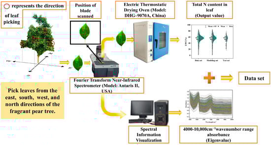
Figure 1.
Data acquisition flow chart.
2.4. Spectral Data Preprocessing
The process used when utilizing spectral technology to analyze LWC and other relevant features of Korla Xiang pear leaves is illustrated in Figure 2. The original spectral data often exhibit issues such as baseline deviation, noise interference, and significant differences in absorbance, which severely affect the accuracy of the subsequent feature extraction and model construction. Spectral pretreatment methods can effectively address these problems. Preprocessed data were used to generate correlation images, evaluate curve smoothness, noise levels, and scattering effects, eliminate background interference, and highlight spectral features related to LWC. This process facilitates the screening of the optimal preprocessing method. Below, several commonly used spectral pretreatment methods are introduced in detail.
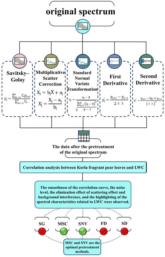
Figure 2.
Pretreatment flow chart.
SG convolution smoothing is primarily based on polynomial fitting. It performs local polynomial fitting for spectral data within a specific window width to achieve smooth processing of spectral curves and reduce the impact of noise and local fluctuations on the data. Additionally, it ensures that the overall trend of the spectrum remains unchanged as much as possible [24]. SG smoothing effectively enhances the smoothness of spectral images, although its direct contribution to improving the correlation between LWC and spectra is relatively limited. However, it creates a stable foundation for subsequent analysis. The formula is as follows:
In this formula, represents the given spectral data sequence for i = 1, 2, …, n; is the data point after convolution smoothing with the Savitzky–Golay filter (where j corresponds to the central position within the window) ; m is the window width (m is usually an odd number); and is the weight coefficient related to the polynomial fitting coefficients.
MSC is used to cope with the scattering effect caused by factors such as sample particles, distribution conditions, and changes in light range. This effect will cause the spectrum to generate a baseline offset and an overall shape change [25]. The principle is based on the assumptions of the ideal spectral shape of all samples, though there are differences in strength due to factors such as scattering. Through correction, the spectrum of all samples can achieve better consistency in strength, thereby eliminating scattering effects. The differences are highlighted through component-related spectral characteristics. The formula is as follows:
represents the average spectrum of all sample spectra. Assuming each sample spectrum contains P wavelength points , where denotes the mean absorbance value of all samples at the i wavelength point represents the spectral value of each individual sample, is the regression coefficient obtained from linear regression fitting, andis the intercept term obtained from the linear regression fitting.
The Standard Normal Variate (SNV) method normalizes the spectrum by subtracting its own mean from each spectrum and dividing by its own standard deviation [26].
The FD (Formula (6)) and SD (Formula (7)) are based on the principle of calculus. The first derivative or second derivative of the spectral data is used to highlight the subtle changes in the spectrum, such as the positional change of the reflection peak and the valley. The derivative transformation can amplify the characteristics of the spectral curve at the slope change, making it easier to identify the less significant features, which is helpful to better extract the feature information. However, these two transformation methods are sensitive to noise. When the derivative transformation is performed in the spectral region with weak signal intensity, the noise can be easily amplified. Therefore, in practical applications, it is often necessary to combine appropriate noise reduction measures to ensure the accuracy of the results [27]. The formula is as follows:
is the discrete sequence of the spectral data (), and is the wavelength interval.
2.5. Spectral Feature Extraction
Given the high dimensionality of spectral data, feature extraction is crucial for identifying relevant bands. Two algorithms were employed: CARS combines Monte Carlo sampling with partial least squares (PLS) regression to select wavelength variables contributing significantly to target variables [28]. It gradually screens the wavelength variables that contribute to the target variables using multiple random sampling and an adaptive weighted process based on the PLS regression coefficient, while simultaneously eliminating those variables with fewer contributions to prediction or strong interference. During each sampling process, the wavelength variables are given different weights based on the size of the PLS regression coefficient. Variables with large weights are considered to be more correlated with the target variables and more important. Throughout the weighted process, the performance is stable, and important variables are used as feature variables to achieve effective feature selection. The SPA is a specialized method for variable selection, with its core objective being to screen out a minimal set of spectral wavelength variables from a large pool [29]. Based on the principle of vector projection, the SPA employs iterative calculations to ensure that the selected variable subset maximizes the information related to the target variable while minimizing collinearity among the variables. This results in a final set of variables that are both representative and independent, making them more suitable for building accurate and robust prediction models.
2.6. Modeling Algorithm
Based on the aforementioned hyperspectral data processing, three machine learning regression algorithms—RFR, SVR, and BP—were utilized to construct an LWC estimation model for Korla Xiang pear.
RFR [30] has obvious advantages, including the ability to handle high dimensional data, strong robustness to noise and outliers, excellent nonlinear modeling capabilities, and good stability and generalization performance, making it suitable for various regression scenarios [31]. In this study, the key parameters include the number of decision trees (n_estimators), the maximum number of features for each tree (max_features), and the minimum number of samples required to split a node (min_samples_split), among others. The range for n_estimators is set to 100–1000 based on the comprehensive analysis by Probst et al. [32], who demonstrated that increasing the number of trees beyond 1000 provides diminishing returns in most practical applications. The max_features parameter ranges from “auto” to the total number of features, following the recommendations of Breiman [33], the original developer of Random Forests, who suggested that this approach typically yields optimal results. The range for min_samples_split is set to 2–5, consistent with the findings of Díaz-Uriarte and Alvarez de Andrés [34], who systematically evaluated parameter settings for Random Forests in high dimensional data analysis.
SVR [35], based on kernel statistical theory, transforms the sample space into a high dimensional or infinite-dimensional feature space via nonlinear mapping, converting nonlinear separable problems in the original sample space into linear separable problems in the feature space. The algorithm exhibits strong robustness to noise and outliers, excellent nonlinear modeling capabilities, and superior performance in handling high dimensional data with strong generalization abilities, making it widely applicable to various regression problems [36]. In this study, the radial basis function was selected as the kernel function, and the penalty coefficient (C) and kernel function parameter (γ) were optimized using grid search. The penalty coefficient (C) was set in the range of 0.2–0.4, and the kernel function parameter (γ) was set in the range of 0.1–500 to ensure optimal model performance.
BP [37] neural networks are widely used in nonlinear modeling and data prediction. They consist of input, output, and intermediate hidden layers, with their learning process encompassing two key steps: forward propagation and backpropagation. During forward propagation, input data sequentially pass through the input layer, hidden layer(s), and output layer for processing. If there is an error between the predicted output and actual data, the backpropagation process is triggered, adjusting neuron weights layer by layer using gradient descent until the error meets the predetermined threshold [38]. In this study, an empirical formula (Equation (7)) was used to define an appropriate range for the number of nodes in the hidden layer. Grid search determined the optimal number of nodes in each hidden layer, with two hidden layers containing the same number of neurons adopted. The iterations were set to 1000, the learning rate was 0.01, and the training target was 1 × 10−⁶ to optimize model performance. The formula is as follows:
where q represents the number of nodes in the hidden layer, k represents the number of input layer cells, m is the number of output layer cells, and α is a constant within the model [1,10].
2.7. Model Evaluation Method
The regression algorithm used in this study was implemented in the MATLAB 2024bsoftware environment. In view of the limited number of samples obtained during a single growth stage, the cross-validation (CV) method was used to verify the model built. This method was derived from the research carried out by Stone [39] in 1976. During the specific CV process, a sample is used as a test set for iteration. The determination of the model parameters is obtained through a comprehensive comparison after multiple training iterations. The results provided are considered to be the expected values obtained from training on the entire dataset. In order to evaluate the performance of the model, we used the R2, the RMSE, and the RPD as the evaluation indicators. The closer R is to unity, the higher the degree of fit between the model and the data; an RMSE value closer to 0 indicates that the model demonstrates excellent predictive accuracy, as evidenced by the tight distribution of forecast values around the ideal prediction line of 1:1, with 95% of predictions falling within ±5% of actual values. According to Zhu et al.’s [40] study conducted in 2020, when RPD ≤ 1.4, the model is determined to be unable to accurately predict the sample; if 1.4 ≤ RPD < 2, the model is considered to be moderately effective and can be used for rough evaluation; and when RPD ≥ 2, the model is considered to have excellent prediction capabilities. The specific calculation formulas of R2, RMSE, and RPD are shown in Formulas (8)–(10), respectively.
where n is the sample size; and are the actual value and the predicted value of Korla fragrant pear LWC, respectively; is the average value of the actual Korla fragrant pear LWC; and is the standard deviation of the LWC measurement value of Korla fragrant pear.
3. Results and Analysis
3.1. Sample Collection Data Statistics
In the process of model construction and subsequent testing, to ensure that both the modeling and testing datasets accurately capture the inherent distribution characteristics of the entire dataset, we employed a scientifically robust data partitioning method. This approach effectively mitigates biases caused by specific data distributions, thereby enhancing the model’s generalization capability. Specifically, the dataset was divided according to a predefined ratio, with 75% of the total samples allocated to the modeling dataset for model construction and the remaining 25% reserved for the testing dataset to evaluate model performance.
For the two distinct growth stages of Korla fragrant pear, samples were carefully selected based on the aforementioned principles. During the S1 growth stage, 252 samples were assigned to the modeling dataset, while 108 samples were allocated to the testing dataset. Similarly, for the S2 growth stage, 137 samples were included in the modeling dataset, and 58 samples were allocated to the testing dataset. Figure 3 illustrates the distribution of samples across the modeling and testing datasets for both growth stages.
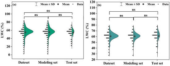
Figure 3.
LWC distribution in different stages of Korla fragrant pear: (a) LWC distribution in the late stage of fruit expansion, (b) LWC distribution in the early stage of maturity.
From Figure 3, the mean and SD values for each growth stage can be derived. In the S1 stage, the LWC in the modeling dataset ranged from 4.88% to 83.45%, with an SD of 11.33%. In the testing dataset, the LWC ranged from 22.03% to 74.29%, with an SD of 9.70% (Figure 3a). For the S2 stage, the LWC in the modeling dataset ranged from 28.77% to 76.52%, with an SD of 6.09%, while in the testing dataset, the LWC ranged from 30.86% to 77.55%, with an SD of 8.32% (Figure 3b).
The analysis of the mean and SD values between the modeling and testing datasets for both growth stages reveals only minor differences. This outcome strongly demonstrates that the dataset partitioning is both reasonable and scientifically sound, meeting the requirements for subsequent model construction and performance evaluation. This careful partitioning lays a solid data foundation for the successful progression of the research.
3.2. Spectral Collection Data Visualization
The original spectral data usually have problems such as noise interference, baseline drift, abnormal samples, high dimensionality and redundant information, uneven sample distribution, and overlapping spectral features. These problems may affect data quality and model performance. The Mahalanobis distance method can effectively detect abnormal samples, improve data quality, enhance model robustness, and consider data distribution characteristics to more accurately measure the distance between samples. Therefore, the Mahalanobis distance method was used in this study to process the original data.
As illustrated in Figure 4, the absorbance values exhibit a complex trend across the entire wavelength range (4000 cm−1 to 10,000 cm−1). The absorbance values cover a wide dynamic range from 0 to 2.0, indicating significant variations in the light absorption capacity of the material or system under investigation within this spectral region. In the 4000 cm−1 to 5000 cm−1 range, the absorbance values gradually increase from a relatively low baseline. Notably, some curves exhibit a steep rise in this interval, suggesting the presence of specific absorption mechanisms or material components that interact strongly with light in this wavelength range.
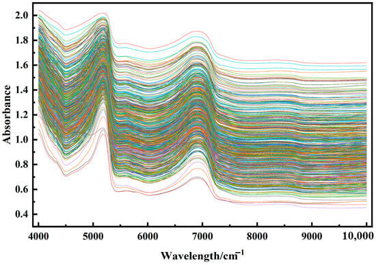
Figure 4.
Visualization of near-infrared original spectra of Korla fragrant pear leaves.
The 5000 cm−1 to 6000 cm−1 region displays more intricate curve shapes, with distinct peaks and valleys observed across multiple curves. This complexity likely arises from the diverse vibrational and rotational modes of molecular structures or chemical bonds within the material, leading to varied light absorption characteristics. The differences in the colored curves in this region may reflect subtle variations in molecular structure or composition among the samples.
In the 6000 cm−1 to 8000 cm−1 range, the absorbance curves generally exhibit a fluctuating trend. Although the overall absorbance decreases, the decline is not monotonic, with localized peaks and valleys still present. This suggests that, despite the overall reduction in absorption capacity, certain wavelengths still exhibit enhanced absorption, possibly due to the presence of specific functional groups or chemical bonds within the material.
Finally, in the spectral range of 8000 cm−1 to 10,000 cm−1, the absorbance values are relatively low with smoother spectral curves, indicating weaker light absorption by the material in this short-wavelength region. This phenomenon can be attributed to the higher photon energy in this range, which exceeds the required energy thresholds for effectively exciting most molecular transitions or chemical bond vibrations in the material.
3.3. Spectral Processing
Figure 5 illustrates the original spectral curves and their mathematical transformations for Korla fragrant pear leaf samples. As shown in Figure 5a, the original absorbance (A) varies significantly among samples, with noticeable baseline shifts and tilts. These variations can be attributed to differences in light absorption characteristics and optical path lengths within the leaves. After applying SG convolution smoothing Figure 5b, the spectral curves become more centered, though the overall trend remains largely unchanged. Following MSC and SNV Figure 5c,d treatments, the differences in absorbance are significantly reduced, resulting in more concentrated and consistent spectral curves.
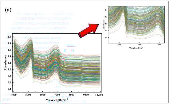
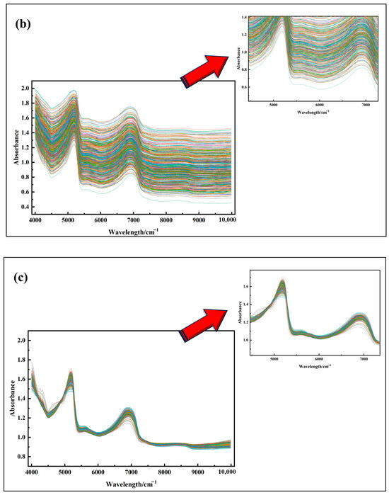
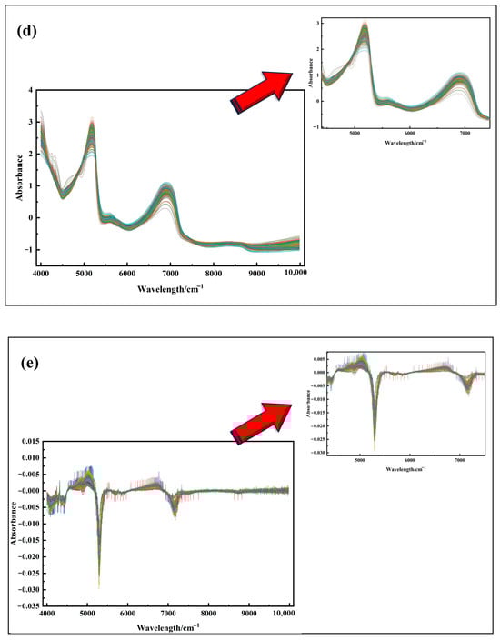
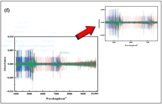
Figure 5.
(a) Spectral images with outliers removed; (b) SG convolution smoothing preprocessing; (c) MSC preprocessing; (d) SNV preprocessing; (e) FD processing; (f) SD processing.
These results demonstrate that MSC and SNV effectively address spectral offset issues, eliminate background interference and noise, and enhance spectral features, laying a solid foundation for the more accurate identification of characteristic wavelengths. In contrast, FD and SD transformations Figure 5e,f excel at highlighting subtle spectral changes, such as the positions of reflection peaks and valleys, thereby reducing background interference and improving feature extraction accuracy. However, in Figure 5e,f, a burr phenomenon is observed in specific wavelength ranges, primarily due to weak signal strength in those regions, which amplifies noise during the derivative conversion process. In summary, each spectral preprocessing method has unique characteristics and plays a vital role in analyzing Korla fragrant pear leaf spectra, offering diverse perspectives and effective data processing approaches for subsequent research and analysis.
3.4. Correlation Analysis Between Korla Fragrant Pear Leaves and LWC
Based on the actual measured LWC data from two key stages of Korla fragrant pear fruit development, the correlation between absorbance and LWC was analyzed before and after mathematical transformations of the spectral data. The results are shown in Figure 6. The correlation analysis between Korla fragrant pear LWC and different transformed spectra revealed diverse characteristics and trends. In the original spectrum (Figure 6a), fluctuations are evident, with distinct peaks and troughs. While these features may relate to LWC, the presence of baseline shifts, tilts, and various interference factors makes it challenging to directly and accurately extract relevant information.
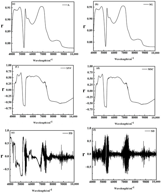
Figure 6.
Correlation between LWC of Korla fragrant pear and different transformation spectra. (a) Original spectrum (b) SG convolution smoothing spectra (c) MSC treatment spectra (d) SNV treatment spectrum (e) FD transform spectrum (f) SD transform spectra.
The purpose of SG convolution smoothing is to enhance the smoothness of the spectrum. However, as shown in the correlation diagram (Figure 6b), there is no significant difference compared to the original spectrum, suggesting that SG smoothing primarily acts as a filter. While its effect on improving the correlation between LWC and spectral data is limited, it provides a stable foundation for subsequent analysis. In contrast, the MSC-treated spectrum (Figure 6c) and SNV-treated spectrum (Figure 6d) show significantly reduced absorbance differences, higher spectral concentrations, and more consistent curve characteristics. These methods effectively eliminate scattering and background interference, highlighting spectral features related to LWC, which facilitates the exploration of their correlation and provides a robust data basis for establishing quantitative analysis models.
The FD-transformed spectrum (Figure 6e) and SD-transformed spectrum (Figure 6f) excel at emphasizing subtle changes, reducing background interference, and improving feature extraction accuracy. However, due to weak signal strength in certain spectral regions, noise is amplified during the derivative conversion process, resulting in burrs. To address this, noise reduction measures should be incorporated to ensure accurate and reliable results.
Based on these findings, this study will focus on exploring correlations and screening characteristic wavelengths using MSC, SNV, and other preprocessed data. By refining and confirming relevant spectral characteristics and optimizing the data processing workflow, this research aims to provide a scientific foundation and practical guidance for developing a rapid detection model for LWC in Korla fragrant pear.
3.5. Selection of the LWC Feature Zones of Korla Fragrant Pear
The LWC feature zones of Korla fragrant pear during the critical fruit development stages (S1 and S2) exhibit significant differences, as clearly illustrated in the corresponding images. The horizontal axis of the images represents wavelengths (wavelength/cm−1), ranging from 4000 to 10,000 cm−1.
During the S1 stage (Figure 7a), the SNV-SPA feature bands, represented by green dots, are primarily concentrated around 5000 cm−1, 6000 cm−1, and 7000 cm−1, indicating specific correlations with LWC. The MSC-SPA feature bands, depicted by blue dots, are distributed around 5500 cm−1 and 7500 cm−1, reflecting the unique spectral characteristics of the Korla fragrant pear LWC. The SNV-CARS feature bands, shown as red dots, cover a broader range around 4500 cm−1, 5500 cm−1, and 8000 cm−1, suggesting a wider association with LWC. The MSC-CARS feature bands, marked by black dots, are concentrated near 6000 cm−1 and 7000 cm−1, highlighting their importance within specific wavelength ranges.
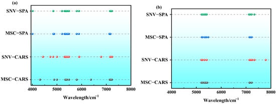
Figure 7.
The characteristic wave position distribution screened by different feature screening algorithms: (a) S1 period; (b) S2 period.(Green line: SNV–SPA algorithm features; Blue line: MSC–SPA algorithm features; Red Line: SNV–CARS Algorithm Features; Black Line: MSC–CARS Algorithm Feature).
In the S2 stage (Figure 7b), the SNV-SPA green dots are mainly located around 5500 cm−1 and 7000 cm−1. Compared to the S1 stage, the feature band near 5000 cm−1 disappears, and new positions emerge, reflecting changes in the growth characteristics of Korla fragrant pear. The MSC-SPA blue dots are predominantly located around 6000 cm−1 and 7500 cm−1, with the feature band near 5500 cm−1 disappearing and shifting towards longer wavelengths, indicating physiological and spectral response changes in Korla fragrant pear. The SNV-CARS red dots are distributed near 4500 cm−1, 6000 cm−1, and 8500 cm−1, with the emergence of a new feature band at 8500 cm−1 demonstrating dynamic changes in the characteristic wavelength zones. The MSC-CARS black dots are fewer in number, mainly around 7000 cm−1, showing a more concentrated distribution and positional changes.
Comparing the images from both stages, it is evident that the physiological characteristics, chemical composition, and spectral interactions of Korla fragrant pear leaves undergo dynamic changes during growth. These findings provide valuable references for researchers to optimize spectral models according to the characteristics of different growth stages, thereby improving the accuracy and reliability of LWC prediction. This, in turn, offers scientific support and technical guarantees for precise irrigation and growth monitoring in agricultural production.
3.6. Korla Fragrant Pear LWC Model Establishment
Figure 8 illustrates the performance indicators of the LWC predictive model for Korla fragrant pear, comprising four subfigures labeled as Figure 8a–d. Each subfigure features three curves representing distinct predictive models: RFR (denoted by a black dotted line), BP (indicated by a red dotted line), and SVR (represented by a blue dotted line). The x-axis of each subfigure corresponds to various feature selection methods, namely, MSC-CARS, SNV-CARS, MSC-SPA, and SNV-SPA. The y-axis in Figure 8a,c displays the coefficient of determination (R2), whereas Figure 8b,d depict the RMSE.
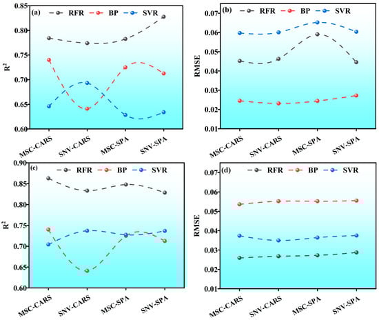
Figure 8.
Modeling results: (a) S1 period R2; (b) S1 period RMSE; (c) S2 period R2; (d) S2 period RMSE.
In Figure 8a, the RFR model demonstrates high and stable R2 values across different feature selection methods, consistently exceeding 0.75. The peak R2 value, nearing 0.85, is achieved using the SNV-SPA method, indicating robust predictive capability, minimal sensitivity to feature selection, and excellent stability and generalization. Conversely, the BP model exhibits significant variability in R2 values. While it achieves a higher R2 value of approximately 0.75 under the MSC-CARS method, this value drops to around 0.65 with the SNV-CARS method, highlighting the model’s sensitivity to feature selection. The SVR model also shows variability in R2 values across different methods, generally lower than those of the RFR model. It performs relatively well under the MSC-SPA method but is less effective than the RFR model overall.
Comparing Figure 8a,c, the RFR model maintains small variations in R2 values and better stability across both periods. The BP model shows reduced variability in Figure 8c compared to Figure 8a, though some fluctuations persist. The SVR model’s R2 values follow a similar trend in both periods, performing well under certain feature selection methods but poorly under others.
In Figure 8b, the RFR model’s RMSE values are consistently low and stable, all below 0.7%, indicating minimal deviation from actual values and high predictive accuracy. The BP model’s RMSE values remain around 0.6% across different methods, suggesting consistent performance in predictive error despite fluctuations in R2 values. The SVR model’s RMSE values vary more significantly, generally higher than those of the RFR model, with some values nearing 0.8% under certain methods, indicating larger prediction errors and a need for improved accuracy.
When comparing Figure 8b,d, the RFR model’s RMSE values show little change, maintaining stable predictive accuracy. The BP model’s RMSE values in Figure 8d are similar to those in Figure 8b, indicating consistent error stability across periods. The SVR model’s RMSE values exhibit a similar trend in both periods, with some fluctuations and generally higher error levels.
3.7. Model Selection and Verification
To further refine the model selection process, a comprehensive validation of all models was conducted. Figure 9 presents the validation results of the combined models constructed using each algorithm, comprising a total of 12 subplots. In each subplot, green scatter points represent the data points, the black line denotes the fitted regression line, and key statistical metrics—including the coefficient of R2, RMSE, and RPD—are provided below each subplot.
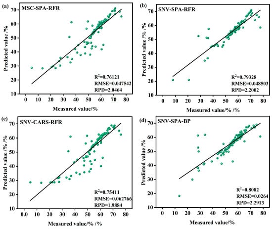
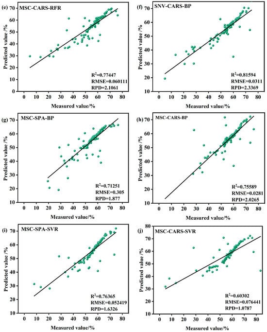
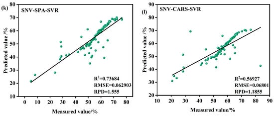
Figure 9.
Model validation in the S1 period. (a) MSC-SPA-RFR model validation (b) SNV-SPA-RFR model validation (c) SNV-CARS-RFR model validation (d) SNV-SPA-BP model validation (e) MSC-CARS-RFR model validation (f) SNV-CARS-BP model validation (g) MSC-SPA-BP model validation (h) MSC-CARS-BP model validation (i) MSC-SPA-SVR model validation (j) MSC-CARS-SVR model validation (k) SNV-SPA-SVR model validation (l) SNV-CARS-SVR model validation.
Among the subplots, the models based on the RFR algorithm demonstrate strong performance in most cases. For instance, the SNV-CARS-BP model achieves an R2 value of 0.81594, indicating an excellent fit, with an RMSE of 0.0311%, reflecting minimal prediction error, and an RPD of 2.3369, highlighting robust predictive capability and stability. Similarly, the SNV-SPA-BP model performs well, with an R2 of 0.8082, an RMSE of 0.0264%, and an RPD of 2.2913. In contrast, certain RFR-based models, such as the SNV-SPA-RFR model, exhibit slightly lower performance, with an R2 of 0.79328, an RMSE of 0.048503%, and an RPD of 2.2002. Another RFR model shows an R2 of 0.77447, an RMSE of 0.060111%, and an RPD of 2.1061, indicating room for improvement.
The SVR models, such as the MSC-SPA-SVR model, display comparatively weaker performance, with an R2 of only 0.76365, an RMSE of 0.052419%, and an RPD of 1.6326, reflecting similar limitations in predictive accuracy.
From the subplots and associated statistical metrics, it is evident that models based on the BP generally outperform the others in most cases, particularly in terms of the coefficient of R2, RMSE, and RPD. In summary, the SNV-CARS-BP model during the S1 period emerges as the most suitable choice for predicting the LWC of Korla fragrant pears.
Figure 10 presents the validation results of the combined models constructed by each algorithm during the S2 period, comprising 12 subplots. The horizontal and vertical axes represent the measured and predicted percentages, respectively. Each subplot includes green scatter points, a black fitted regression line, and key statistical metrics—such as the coefficient of determination (R2), root mean square error of prediction (RMSEP), and RPD—displayed below.
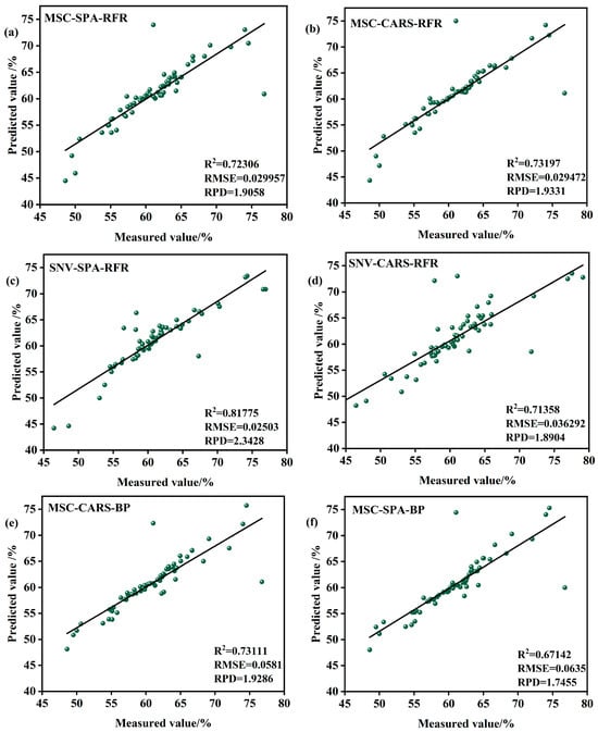
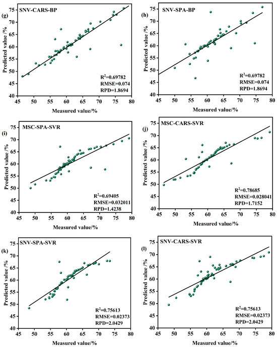
Figure 10.
Model validation in the S2 period. (a) MSC-SPA-RFR model validation (b) MSC-CARS-RFR model validation (c) SNV-SPA-RFR model validation (d) SNV-CARS-RFRmodel validation (e) MSC-CARS-BPmodelvalidation (f) MSC-SPA-BPmodelvalidation (g) SNV-CARS-BPmodel validation (h) SNV-SPA-BP model validation (i) MSC-SPA-SVR model validation (j) MSC-CARS-SVR model validation (k) SNV-SPA-SVR model validation (l) SNV-CARS-SVRmodel validation.
Among the models, those based on RFR demonstrate strong performance. For instance, the SNV-SPA-RFR model achieves an R2 of 0.817756, indicating an excellent fit, with an RMSE of 0.02503%, reflecting minimal deviation, and an RPD of 2.3428, showcasing robust predictive capability and stability. Similarly, the MSC-CARS-RFR model, with an R2 of 0.79331, an RMSEP of 0.02933%, and an RPD of 1.9331, also provides valuable predictive insights.
In contrast, models based on the BP exhibit mixed performance during the S2 period. While some BP-based models, such as SNV-CARS-BP and MSC-SPA-BP, show relatively lower R2 values, higher RMSEP, and reduced RPD, indicating limitations in fitting accuracy and predictive performance, others demonstrate potential but require further optimization. Similarly, SVR models, such as MSC-CARS-SVR and SNV-SPA-SVR, display scattered data points, with R2 values of 0.78685 and 0.76365, RMSEP values of 0.028041% and 0.030419%, and RPD values of 1.7152 and 1.6326, respectively. These results suggest that SVR models also need improvement or exploration of alternative methods to enhance their predictive accuracy.
In summary, the SNV-SPA-RFR model during the S2 period is well suited for data prediction, offering a balance of high R2, low RMSEP, and strong RPD. However, the performance of BP- and SVR-based models highlights the need for further optimization or exploration of new methodologies to improve their predictive capabilities. These findings provide valuable insights for subsequent research and model refinement, contributing to a deeper understanding of the performance characteristics and applicability of each algorithm in this context. Practical applications should consider these results comprehensively to select the most appropriate model for specific predictive tasks.
Model accuracy is a critical factor in determining the usability of a predictive model. To further validate the constructed models, we assessed the relative deviation between the actual values and the predicted values, which serves as a key indicator of model accuracy. As illustrated in Figure 11, the relative deviations for the SNV-CARS-BP model during the S1 period and the SNV-SPA-RFR model during the S2 period are notably small, ranging from 0.00041% to 2.96649% and 0.00039% to 0.13751%, respectively. These deviations fall well within the acceptable threshold of less than 5%, demonstrating that the LWC prediction models for Korla fragrant pear leaves exhibit high accuracy.
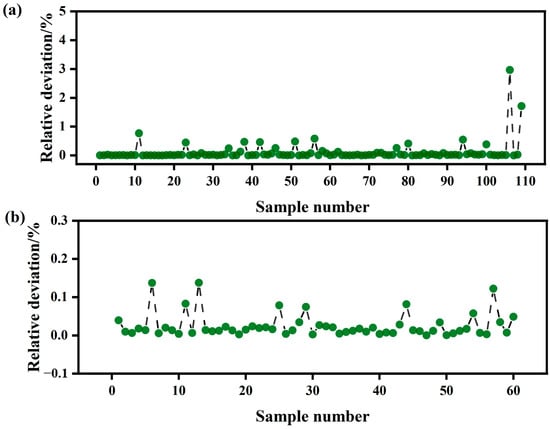
Figure 11.
Standard deviation of the measured and predicted values of the LWC of the validation set samples: (a) the S1 period; (b) the S2 period.
This result confirms the reliability of the models and their potential for practical applications in predicting the water content of Korla fragrant pear leaves. The minimal deviations further validate the robustness and precision of the selected models, highlighting their suitability for real-world use.
4. Discussion
In this study, a random splitting method was employed during the sample collection stage to partition the dataset, ensuring that both the modeling and test datasets accurately capture the inherent distribution characteristics of the data and enhance the model’s generalization ability. Specifically, in the S1 growth stage of Korla fragrant pear, 252 samples were allocated to the modeling dataset, while 108 samples were designated for the test dataset. Similarly, in the S2 stage, 137 and 58 samples were selected for the modeling and test datasets, respectively.
The distribution range and standard deviation of LWC were analyzed for both stages. In the S1 stage, the LWC distribution of the modeling set ranged from 4.88% to 83.45%, with a standard deviation of 11.33, while the test set ranged from 22.03% to 74.29%, with a standard deviation of 9.70. The corresponding data for the S2 stage also exhibited reasonable differences, with minimal discrepancies in the mean values and standard deviations between the modeling and test sets. These results strongly validate the rationality and scientific rigor of the dataset partitioning method. A well-partitioned dataset serves as the cornerstone for constructing high quality models in subsequent analyses [41]. Compared with traditional methods, which usually rely on hand designed feature extraction methods, machine learning algorithms can well reflect the characteristics of RFR, SVR, and BP that can effectively process high dimensional data (such as spectral data), extract key information through feature selection and dimensionality reduction techniques, and reduce the interference of redundant data. By adopting this approach, the model is exposed to a diverse range of data during training, thereby avoiding issues such as overfitting caused by data bias and ensuring robust predictive performance when applied to new data [42]. However, it is worth noting that while the current partitioning method has yielded satisfactory results, the sample collection process in practical applications may be influenced by various factors, such as limitations in sampling sites and the inherent randomness of individual samples. The traditional method is sensitive to noise and outliers, and it is easy to overfit or underfit. However, RFR has high robustness to noise and outliers, which can effectively avoid overfitting problems. SVR can also improve the generalization ability of the model through regularization technology. In the future, expanding the sampling range to include Korla fragrant pear samples from a wider variety of growth environments could enhance the dataset’s representativeness and further optimize model performance.
The spectral acquisition data exhibit complex trends. Within the range of 4000–10,000 cm−1, the absorbance varies significantly across different intervals, reflecting the diverse and intricate light absorption characteristics of the material [43]. Each spectral preprocessing method has its own strengths and limitations. SG convolution smoothing enhances spectral smoothness but has a limited effect on improving the correlation between LWC and spectral data. In contrast, MSC and SNV processing significantly reduce absorbance differences, enhance spectral features, and effectively address issues such as spectral offset and background interference. While FD and SD transformations excel at highlighting subtle changes to aid feature extraction, they tend to amplify noise and produce burrs in regions with weak signals.
In practical research, the comprehensive application of various preprocessing methods offers diverse perspectives and effective tools for subsequent analysis. However, this also highlights the need to carefully weigh the characteristics of different methods and research objectives when selecting preprocessing techniques. For instance, if the focus is on noise reduction and obtaining more stable spectral features, MSC and SNV methods may be more suitable. As demonstrated by Chenbo et al. [44] in their construction of a hyperspectral monitoring model for oat grain β-glucan content, the model based on SNV-transformed spectra and SPA–multiple linear regression (SPA-MLR) achieved the highest accuracy, enabling effective hyperspectral monitoring of oat grain β-glucan content.
The wavelength range of near-infrared (NIR) light spans from 780 nm to 2500 nm, enabling it to penetrate various organic substances and interact with chemical bonds. The O-H bond in water molecules (H2O) exhibits characteristic absorption bands in the NIR region, particularly near 1450 nm and 1940 nm. When NIR light irradiates fruit tree tissue, photons are absorbed by the O-H bond, causing a transition in the molecular vibration energy levels and increasing vibrational energy. By measuring the light absorption intensity at different wavelengths, the absorption spectrum of water molecules can be obtained, with peaks corresponding to the vibrational modes of the O-H bond.
However, near-infrared spectroscopy detection may encounter interference from other functional groups, such as O-H bonds in alcohols and phenols, as well as N-H and C-H bonds, which also exhibit absorption bands in the near-infrared region. To mitigate these interferences, feature selection can be applied after spectral preprocessing to identify wavelength points most relevant to the target variable, such as moisture content. For instance, prioritizing water-specific absorption bands (e.g., 1450 nm and 1940 nm) can enhance the signal of water molecules while minimizing the influence of other functional groups. This approach significantly improves the accuracy and specificity of detection, providing reliable support for the application of near-infrared spectroscopy in analyzing fruit tree water content.
In spectral analysis, accurately capturing subtle changes often requires advanced preprocessing techniques. FD and SD transformations, particularly when combined with noise reduction measures, play a crucial role in enhancing spectral features. Previous studies have demonstrated the effectiveness of these approaches; for instance, Li et al. [45] analyzed β-glucan and total starch in oats using spectral data and chemometric methods. Their results showed varying model performance across components, with the total starch model achieving optimal results after SD-SPA treatment (Rp2 = 0.768, RMSEP = 2.057% relative to a mean response value of 78.3%). This represents a prediction error of ±2.63% of the measured range and a 62.5% improvement over previous approaches. These findings underscore the importance of derivative transformations in spectral modeling, which we have further developed in our current study. The findings demonstrate that this technology enables accurate quantification and provides an effective approach for oat quality detection. Furthermore, with the ongoing advancement of spectral technology, exploring new and more targeted spectral preprocessing methods, or refining and optimizing existing ones, holds promise for further enhancing spectral data quality. This improvement would lay a stronger foundation for more accurate LWC prediction models.
Notably, the selection of LWC characteristic bands for Korla fragrant pear during the S1 and S2 periods revealed significant differences. The positions of characteristic bands identified by various feature screening algorithms varied between the two stages. For instance, during the S1 period, the SNV-SPA characteristic bands were concentrated around 5000 cm−1, 6000 cm−1, and 7000 cm−1, with corresponding shifts observed in the S2 period. These variations reflect the dynamic changes in leaf physiological characteristics, chemical composition, and spectral interactions throughout the growth of Korla fragrant pear.
Accurately understanding these characteristic band differences is crucial for optimizing spectral models. Researchers can adjust model parameters or select appropriate model structures based on the unique characteristics of different growth stages, thereby enhancing the accuracy and reliability of LWC predictions. However, it is important to recognize that current feature band selection methods rely on existing data and algorithms, which may have inherent limitations. In the future, hyperparameter optimization research can be enhanced through multiple approaches to improve the performance and practical value of the Korla fragrant pear LWC prediction model. First, more efficient and intelligent optimization methods, such as Bayesian optimization or reinforcement learning-based algorithms, can be explored to reduce computational costs and enhance search efficiency. Second, by integrating dynamic feature selection methods, the feature selection strategy can be automatically adjusted according to the physiological characteristics of Korla fragrant pear at different growth stages, further improving the model’s adaptability.
In the model development process, the performance of machine learning models is significantly influenced by the selection of hyperparameters. Optimizing these hyperparameters directly impacts the model’s generalization ability and prediction accuracy [46]. To ensure optimal model performance, grid search and cross-validation were employed in this study to fine-tune the hyperparameters of RFR, SVR, and BP. The results are illustrated in Figure 12a,b.
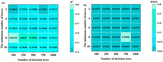
Figure 12.
Parameter selection. (a) Change in R2 in the process of decision tree and cotyledon number change in SNV-SPA-RFR model during S2 period of Korla fragrant pear; (b) change in RMSE during the change in decision tree and cotyledon number in SNV-SPA-RFR model during S2 period of Korla fragrant pear; (c) change in R2 in the process of decision tree and cotyledon number change in SNV-CARS-SVR model during S2 period of Korla fragrant pear; (d) change in RMSE in the process of decision tree and cotyledon number change in SNV-CARS-SVR model during S2 period of Korla fragrant pear; (e) changes in R2 and RMSE in the optimization process of BP model hyperparameters q and α.
For the S2 period of Korla fragrant pear, taking the SNV-SPA-RFR model as an example, R2 exhibits a clear trend, with varying values for the number of decision trees and leaf nodes. When the number of leaf nodes (cotyledons) is set to 8 and the number of decision trees is 100, the model achieves the highest R2 value of 0.81519, indicating optimal accuracy. Additionally, the RMSE reaches its minimum value of 0.02503% at this parameter combination, further confirming the best model fit. Therefore, the optimal parameters for this model are cotyledon = 8 and decision tree = 100.
For the SVR model, the SNV-SPA-RFR model in the S2 period of Korla fragrant pear was used as an example to optimize the hyperparameters C and γ. As shown in Figure 12c,d, R2 exhibits a clear trend, with varying values for C and γ. When C = 0.3 and γ = 0.1, the model achieves the highest R2 value of 0.73719, indicating optimal generalization ability. Additionally, Figure 12c,d illustrate the changes in R2 values corresponding to different C and γ parameters. Consistent with the RMSE heat map, these results further confirm the best model fit under this parameter combination. Therefore, the optimal parameters for this model are C = 0.3 and γ = 0.1.
For the BP model, the SNV-CARS-BP model of the S1 stage of Korla fragrant pear was used as an example, and grid search was employed to determine the optimal constant α. As shown in Figure 12e, variations in the number of q and the constant α result in significant fluctuations in the model’s R2 and RMSE values. Notably, when q = 8 and α = 4, the model achieves the highest R2 value of 0.81594 and the lowest RMSE value of 0.0311%, indicating the best model fit. Therefore, the optimal parameters for this model are q = 8 and α = 4.
During the model selection phase, we compared the performance of RFR (Random Forest Regression), BP (Backpropagation Neural Network), and SVR (Support Vector Regression) under various feature selection methods. The results demonstrated that the RFR model exhibited superior stability and generalization capabilities, with minimal performance variations across different feature selection approaches. Conversely, the BP model showed significant sensitivity to feature selection, leading to substantial performance fluctuations. The SVR model, while also influenced by feature selection, displayed slightly lower overall predictive accuracy compared to RFR.
Further model validation revealed that the SNV-CARS-BP model performed exceptionally well during the S1 stage, while the S2-SPA-RFR model excelled in the S2 stage. Both models maintained low relative deviations between predicted and actual values, confirming their high accuracy, as detailed in Table 1 and Table 2. However, this does not negate the value of other models. Different algorithms may exhibit unique strengths under specific application scenarios or data characteristics. For instance, the BP neural network shows potential in handling complex nonlinear relationships. By optimizing its algorithmic structure to address current limitations, the BP model could achieve enhanced performance in predicting LWC (Leaf Water Content) for Korla fragrant pears. Similarly, refining the kernel functions and parameter configurations of the SVR model may further improve its effectiveness.

Table 1.
S1- and S2-stage model modeling data.
Table 2.
S1- and S2-stage model validation set data.
Our results are consistent with those of several recent studies using machine learning to predict LWC. For example, Li et al. [11] used RFR to analyze hyperspectral data and obtained a result of R2 = 0.85, which is comparable to the result of our SNV-SPA-RFR model (R2 = 0.815). Similarly, Liu et al. [26] used SVR to estimate the LWC of crops, and the reported RMSE was 0.030%, which was slightly higher than the RMSE (0.025%) of our SNV-SPA-RFR model. These comparisons highlight the robustness of our method and its potential for generalization under different crops and conditions. However, unlike previous studies, our work systematically evaluated a variety of preprocessing methods (SG, MSC, SNV, FD, SD) and machine learning algorithms (RFR, SVR, BP) to determine the best combination of LWC predictions for Korla fragrant pear, providing a more comprehensive framework for future research.
This study has obtained important results in the key links of dataset division, spectral preprocessing, feature band selection, model hyperparameter optimization, model selection, and verification. The random splitting method is used to divide the dataset, which ensures that the modeling and test dataset can accurately capture the internal distribution characteristics of the data, improve the generalization ability of the model, and lay the foundation for the subsequent high quality model construction. In terms of spectral preprocessing, SG, MSC, SNV, FD, SD, and other methods have their own advantages and disadvantages. The comprehensive application can provide diversified perspectives and effective means to improve the quality of spectral data. The selection of characteristic bands showed that there were significant differences in the LWC characteristic bands of Korla fragrant pear during the S1 and S2 periods, which reflected the dynamic changes of leaf physiological characteristics during its growth process. Accurately understanding these differences is helpful to optimize the spectral model. The model hyperparameter optimization determines the optimal parameter combination of RFR, SVR, and BP models through grid search and cross-validation, which directly improves the generalization ability and prediction accuracy of the model. These results not only provide a solid foundation for the construction and optimization of Korla fragrant pear LWC prediction models but also highlight directions for future research, which has important theoretical and practical value.
Moreover, practical applications should not rely solely on a single evaluation metric for model selection. It is crucial to consider additional factors such as model complexity, computational efficiency, and interpretability [47]. Future research should explore integrated strategies that leverage the strengths of different models, aiming to develop more robust and versatile LWC prediction models for Korla fragrant pears. Such advancements would provide more precise technical support for agricultural practices, including targeted irrigation and growth monitoring.
In conclusion, this study has made significant progress through a comprehensive analysis of multiple aspects related to Korla fragrant pear LWC. However, there remains ample room for optimization and expansion in various areas. Continued exploration and advancement in the aforementioned directions will further enhance research in this field, ultimately contributing to more effective agricultural production practices.
5. Conclusions
This study explored the LWC of Korla fragrant pear, with the objective of developing a precise and effective LWC prediction model to support agricultural production practices. In the sample collection phase, a random split method was employed to partition the dataset. Samples were selected based on the distinct characteristics of the S1 and S2 growth stages, ensuring a scientifically sound division that underpins subsequent analytical work.
The spectral collection process highlighted the complexities of lighting conditions, and in the spectral processing stage, various techniques such as SG convolution, MSC, SNV, FD, and SD were utilized, each contributing uniquely to the optimization of data quality.
In terms of feature band selection, notable differences were observed between the S1 and S2 periods. These dynamic changes reflect the growth patterns of fragrant pear and provide a basis for refining the spectral model. During the model establishment and selection phase, a comparison was made among RFR, BP, and SVR models. This led to the identification of superior models for different periods, specifically the SNV-CARS-BP model for the S1 period and the SNV-SPA-RFR model for the S2 period, both of which demonstrated high accuracy.
While this study has yielded significant results, there remains scope for enhancement in each segment. Sample collection could be expanded to increase diversity and representativeness; spectral treatment could benefit from the exploration and optimization of new methods; feature band selection could integrate more sophisticated techniques to reveal additional characteristics; and model development could explore fusion strategies or further optimize individual model performances.
Looking ahead, continued research in these directions is anticipated to yield an improved LWC prediction model, thereby aiding in the precise irrigation and growth monitoring of Korla fragrant pear in agricultural practices.
Author Contributions
M.Y.: conceptualization, methodology, data curation, writing—original draft, writing—review and editing; W.F.: conceptualization, methodology, data curation, writing—original draft, writing—review and editing; L.W.: visualization, software; Y.C.: validation, investigation; H.W.: visualization, formal analysis; K.G.: supervision, formal analysis; J.B.: resources, writing—review and editing, project administration, funding acquisition. All authors have read and agreed to the published version of the manuscript.
Funding
The Bingtuan Science and Technology Program (Grant Nos. 2021CB055, 2022CB001-11). The National Natural Science Foundation of China (Grant Nos. 31860528, U2003121). The First Division Science and Technology Project (Grant No. 2022NY03).
Data Availability Statement
The data that support the findings of this study are available from the corresponding author upon reasonable request.
Conflicts of Interest
The authors declare no conflicts of interest.
Abbreviations
| R2 | Coefficient of Determination |
| RMSE | Root Mean Square Error |
| RPD | Ratio of Performance to Deviation |
| RFR | Random Forest Regression |
| BP | Backpropagation |
| SNV | Standard Normal Variate |
| CARS | Competitive Adaptive Reweighted Sampling |
| SPA | Successive Projections Algorithm |
| SG | Savitzky–Golay |
| MSC | Multiplicative Scatter Correction |
| SD | Second Derivative |
| FD | First Derivative |
References
- Kaiser, H.; Sagervanshi, A.; Mühling, K.H. A method to experimentally clamp leaf water content to defined values to assess its effects on apoplastic pH. Plant Methods 2021, 18, 72. [Google Scholar] [CrossRef] [PubMed]
- Wang, R.; He, N.; Li, S.; Xu, L.; Li, M. Spatial variation and mechanisms of leaf water content in grassland plants at the biome scale: Evidence from three comparative transects. Sci. Rep. 2021, 11, 9281. [Google Scholar] [CrossRef]
- Magney, T.S. Hyperspectral reflectance integrates key traits for predicting leaf metabolism. New Phytol. 2024, 246, 383. [Google Scholar] [CrossRef]
- Qi, H.; Luo, J.; Wu, X.; Zhang, C. Application of nondestructive techniques for peach (Prunus persica) quality inspection: A review. J. Food Sci. 2024, 89, 6863–6887. [Google Scholar] [CrossRef]
- Lu, Z.; Lu, R.; Chen, Y.; Fu, K.; Song, J.; Xie, L.; Zhai, R.; Wang, Z.; Yang, C.; Xu, L. Nondestructive Testing of Pear Based on Fourier Near-Infrared Spectroscopy. Foods 2022, 11, 1076. [Google Scholar] [CrossRef] [PubMed]
- Morvan, E.; Kauffmann, B.; Grélard, A.; Loquet, A.; Dixon, A.-J.; Dufourc, E.J.; Rontein, D. Natural crystalline fibers of (E)-(R)-4-thujanol: Green kilogram production from a selected wild thyme. X-ray and NMR characterization of a spiral structure. Ind. Crops Prod. 2022, 187, 115451. [Google Scholar] [CrossRef]
- Xu, J.; Bao, J. Effects of different irrigation amounts on storage quality of Korla fragrant pear fruit under irrigation mode. XinJiang Agric. Sci. 2024, 61, 1696–1709. [Google Scholar] [CrossRef]
- Jiang, W.; Yan, P.; Zheng, Q.; Wang, Z.; Chen, Q.; Wang, Y. Changes in the Metabolome and Nutritional Quality of Pulp from Three Types of Korla Fragrant Pears with Different Appearances as Revealed by Widely Targeted Metabolomics. Plants 2023, 12, 3981. [Google Scholar] [CrossRef]
- Lv, G.; Jin, J.; He, M.; Wang, C. Soil Moisture Content Dominates the Photosynthesis of C3 and C4 Plants in a Desert Steppe after Long-Term Warming and Increasing Precipitation. Plants 2023, 12, 2903. [Google Scholar] [CrossRef]
- Zhou, Z.; Su, P.; Yang, J.; Shi, R.; Ding, X. Warming affects leaf light use efficiency and functional traits in alpine plants: Evidence from a 4-year in-situ field experiment. Front. Plant Sci. 2024, 15, 1353762. [Google Scholar] [CrossRef]
- Li, G.; Long, H.; Zhang, R.; Xu, A.; Niu, L. Photosynthetic traits, water use and the yield of maize are influenced by soil water stability. BMC Plant Biol. 2024, 24, 1235. [Google Scholar] [CrossRef]
- Helyes, L.; Pék, Z.; Lugasi, A. Tomato Fruit Quality and Content Depend on Stage of Maturity. Hortscience 2006, 41, 1400–1401. [Google Scholar] [CrossRef]
- Guo, F.; Feng, Q.; Yang, S.; Yang, W. Estimation of potato canopy leaf water content in various growth stages using UAV hyperspectral remote sensing and machine learning. Front. Plant Sci. 2024, 15, 1458589. [Google Scholar] [CrossRef]
- Zhao, Y.; Si, L.T.; Ouyang, H. Frequency domain analysis method of nonstationary random vibration based on evolutionary spectral representation. Eng. Comput. 2018, 35, 1098–1127. [Google Scholar]
- Zhang, F.; Tang, X.; Li, L. Origins of Baseline Drift and Distortion in Fourier Transform Spectra. Molecules 2022, 27, 4287. [Google Scholar] [CrossRef]
- Vezvaee, A.; Shitara, N.; Sun, S.; Montoya-Castillo, A. Fourier transform noise spectroscopy. NPJ Quantum Inf. 2024, 10, 52. [Google Scholar] [CrossRef]
- Singh, T.; Garg, N.M.; Iyengar, S.R.S. Nondestructive identification of barley seeds variety using near-infrared hyperspectral imaging coupled with convolutional neural network. J. Food Process Eng. 2021, 44, e13821. [Google Scholar] [CrossRef]
- Yu, M.; Bai, X.; Bao, J.; Wang, Z.; Tang, Z.; Zheng, Q.; Zhi, J. The Prediction Model of Total Nitrogen Content in Leaves of Korla Fragrant Pear Was Established Based on Near Infrared Spectroscopy. Agronomy 2024, 14, 1284. [Google Scholar] [CrossRef]
- Bao, J.; Yu, M.; Li, J.; Wang, G.; Tang, Z.; Zhi, J. Determination of leaf nitrogen content in apple and jujube by near-infrared spectroscopy. Sci. Rep. 2024, 14, 20884. [Google Scholar] [CrossRef]
- Ye, R.; Chen, Y.; Guo, Y.; Duan, Q.; Li, D.; Liu, C. NIR Hyperspectral Imaging Technology Combined with Multivariate Methods to Identify Shrimp Freshness. Appl. Sci. 2020, 10, 5498. [Google Scholar] [CrossRef]
- Tang, R.; Li, X.; Li, C.; Jiang, K.; Hu, W.; Wu, J. Estimation of Total Nitrogen Content in Rubber Plantation Soil Based on Hyperspectral and Fractional Order Derivative. Electronics 2022, 11, 1956. [Google Scholar] [CrossRef]
- Xu, X.; Zhao, T.; Ma, J.; Song, Q.; Wei, Q.; Sun, W. Application of Two-Stage Variable Temperature Drying in Hot Air-Drying of Paddy Rice. Foods 2022, 11, 888. [Google Scholar] [CrossRef]
- Langqin, L.; Tao, W.; Guoqing, L.; Wenge, Z.; Rui, Z.; Jun, Y.; Bin, L.; Tiancai, C. A model for soluble protein content detection of walnuts based on near in-frared spectroscopy. J. Fruit. Sci. 2023, 40, 1750–1761. [Google Scholar] [CrossRef]
- Schmid, M.; Rath, D.; Diebold, U. Why and How Savitzky-Golay Filters Should Be Replaced. ACS Meas. Sci. Au 2022, 2, 185–196. [Google Scholar] [CrossRef] [PubMed]
- Xia, C.; Ren, M.; Wang, B.; Dong, M.; Song, B.; Hu, Y.; Pischler, O. Acquisition and analysis of hyperspectral data for surface contamination level of insulating materials. Measurement 2021, 173, 108560. [Google Scholar] [CrossRef]
- Liu, L.; Qi, M.; Li, Y.; Liu, Y.; Liu, X.; Zhang, Z.; Qu, J. Staging of Skin Cancer Based on Hyperspectral Microscopic Imaging and Machine Learning. Biosensors 2022, 12, 790. [Google Scholar] [CrossRef]
- Shi, H.; Yu, P. Using Molecular Spectroscopic Techniques (NIR and ATR-FT/MIR) Coupling with Various Chemometrics to Test Possibility to Reveal Chemical and Molecular Response of Cool-Season Adapted Wheat Grain to Ergot Alkaloids. Toxins 2023, 15, 151. [Google Scholar] [CrossRef]
- Wu, K.; Zhu, T.; Wang, Z.; Zhao, X.; Yuan, M.; Liang, D.; Li, Z. Identification of varieties of sorghum based on a competitive adaptive reweighted sampling-random forest process. Eur. Food Res. Technol. 2024, 250, 191–201. [Google Scholar] [CrossRef]
- Zhang, J.; Rivard, B.; Rogge, D.M. The Successive Projection Algorithm (SPA), an Algorithm with a Spatial Constraint for the Automatic Search of Endmembers in Hyperspectral Data. Sensors 2008, 8, 1321–1342. [Google Scholar] [CrossRef]
- Wu, B.; Ye, H.; Huang, W.; Wang, H.; Luo, P.; Ren, Y.; Kong, W. Monitoring the Vertical Distribution of Maize Canopy Chlorophyll Content Based on Multi-Angular Spectral Data. Remote Sens. 2021, 13, 987. [Google Scholar] [CrossRef]
- Huang, Z.; Liu, Z. A Complex Terrain Simulation Approach Using Ensemble Learning of Random Forest Regression. J. Indian. Soc. Remote Sens. 2022, 50, 2011–2023. [Google Scholar] [CrossRef]
- Probst, P.; Boulesteix, A.-L.; Bischl, B. Tunability: Importance of hyperparameters of machine learning algorithms. J. Mach. Learn. Res. 2019, 20, 1934–1965. [Google Scholar] [CrossRef]
- Breiman, L. Random Forests. Mach. Learn. 2001, 45, 5–32. [Google Scholar] [CrossRef]
- Díaz-Uriarte, R.; Alvarez de Andrés, S. Gene selection and classification of microarray data using random forest. BMC Bioinform. 2006, 7, 3. [Google Scholar] [CrossRef]
- Kagan, C.R.; Arnold, D.P.; Cappelleri, D.J.; Keske, C.M.; Turner, K.T. Special report: The Internet of Things for Precision Agriculture (IoT4Ag). Comput. Electron. Agric. 2022, 196, 106742. [Google Scholar] [CrossRef]
- Zhang, M.; Zhang, X.; Gao, S.; Zhu, Y. Comfort Study of General Aviation Pilot Seats Based on Improved Particle Swam Algorithm (IPSO) and Support Vector Machine Regression (SVR). Appl. Sci. 2023, 13, 9038. [Google Scholar] [CrossRef]
- Chen, Y.; Yang, J.; Zhang, D.; Zhang, K.; Chen, B.; Du, S. Region-aware network: Model human’s Top-Down visual perception mechanism for crowd counting. Neural Netw. 2022, 148, 219–231. [Google Scholar] [CrossRef] [PubMed]
- Zhang, Y.; Wang, K.; Peng, H.; Liu, X.; Huang, Y.; An, H.; Lei, Y. Novel Life Prediction Method of PMMA for Cultural Relics Protection Based on the BP Neural Network. ACS Omega 2023, 8, 47812–47820. [Google Scholar] [CrossRef]
- Stone, M. Cross-Validatory Choice and Assessment of Statistical Predictions (with Discussion). J. R. Stat. Soc. Ser. B 1976, 38, 102. [Google Scholar] [CrossRef]
- Zhu, Z.; Li, T.; Cui, J.; Shi, X.; Wang, H. Non-destructive estimation of winter wheat leaf moisture content using near-ground hyperspectral imaging technology. Acta Agric. Scand. Sect. B Soil Plant Sci. 2020, 70, 1–13. [Google Scholar] [CrossRef]
- Jia, W.; Wang, Y.; Chen, R.; Ye, J.; Li, D.; Yin, F.; Yu, J.; Chen, J.; Shu, Q.; Xu, W. ZCHSound: Open-Source ZJU Paediatric Heart Sound Database With Congenital Heart Disease. IEEE Trans. Biomed. Eng. 2024, 71, 2278–2286. [Google Scholar] [CrossRef] [PubMed]
- Tao, H.; Al-Sulttani, A.O.; Salih Ameen, A.M.; Ali, Z.H.; Al-Ansari, N.; Salih, S.Q.; Mostafa, R.R. Training and Testing Data Division Influence on Hybrid Machine Learning Model Process: Application of River Flow Forecasting. Complexity 2020, 2020, 8844367. [Google Scholar] [CrossRef]
- Erlandsson, M.; Futter, M.N.; Kothawala, D.N.; Köhler, S.J. Variability in spectral absorbance metrics across boreal lake waters. J. Environ. Monit. 2012, 14, 2643–2652. [Google Scholar] [CrossRef] [PubMed]
- Yang, C.; Song, L.; Wang, D.; Hao, S.; Feng, M.; Zhang, M.; Wang, C.; Xiao, L.; Yang, W.; Song, X. Study on hyperspectral monitoring model of β-glucan content in oat grains. J. Food Meas. Charact. 2023, 17, 5134–5143. [Google Scholar] [CrossRef]
- Meenu, M.; Zhang, Y.; Kamboj, U.; Zhao, S.; Cao, L.; He, P.; Xu, B. Rapid Determination of β-Glucan Content of Hulled and Naked Oats Using near Infrared Spectroscopy Combined with Chemometrics. Foods 2022, 11, 43. [Google Scholar] [CrossRef]
- Luo, R.; Li, Y.; Guo, H.; Wang, Q.; Wang, X. Cross-operating-condition fault diagnosis of a small module reactor based on CNN-LSTM transfer learning with limited data. Energy 2024, 313, 133901. [Google Scholar] [CrossRef]
- Wettewa, S.; Hou, L.; Zhang, G. Graph Neural Networks for building and civil infrastructure operation and maintenance enhancement. Adv. Eng. Inform. 2024, 62, 102868. [Google Scholar] [CrossRef]
Disclaimer/Publisher’s Note: The statements, opinions and data contained in all publications are solely those of the individual author(s) and contributor(s) and not of MDPI and/or the editor(s). MDPI and/or the editor(s) disclaim responsibility for any injury to people or property resulting from any ideas, methods, instructions or products referred to in the content. |
© 2025 by the authors. Licensee MDPI, Basel, Switzerland. This article is an open access article distributed under the terms and conditions of the Creative Commons Attribution (CC BY) license (https://creativecommons.org/licenses/by/4.0/).