A Rice-Mapping Method with Integrated Automatic Generation of Training Samples and Random Forest Classification Using Google Earth Engine

Abstract

Accurate mapping of rice planting areas is of great significance in terms of food security and market stability. However, the existing research into high-resolution rice mapping has relied heavily on fine-scale temporal remote sensing image data. Due to cloud occlusion and banding problems, data extraction from Landsat series remote sensing images with medium spatial resolution is not optimal. Therefore, this study proposes a rice mapping method (LR) using Google Earth Engine (GEE), which uses Landsat images and integrates automatic generation of training samples and a machine learning algorithm, with the assistance of phenological methods. The proposed LR method initially generated rice distribution maps based on phenology, and 300 sample points were selected for meta-identification of rice images via an enhanced pixel-based phenological feature composite method (Eppf-CM) utilizing high-resolution imagery. Subsequently, the inundation frequency (F) and an improved sample point statistical feature, i.e., the ratio of change amplitude of LSWI to NDVI (RCLN), were introduced to combine Eppf-CM with combined consideration of vegetation phenology and surface water variation (CCVS) methods, to automate the generation of training data with the aid of phenology. The sample data were optimized by an alternate iterative method involving extraction of neighborhood information. Finally, a random forest (RF) probabilistic model trained by integrating data from different phenological periods was used for rice mapping. To test its performance, we mapped rice distribution at 30 m resolution (“LR_Rice”) across Heilongjiang Province, China from 2010 to 2022, with annual overall accuracy (OA) and Kappa coefficients greater than 0.97 and 0.95, respectively, and compared them with four existing rice mapping products. The spatial distribution characteristics of rice cultivation extracted by the LR algorithm were accurate and the performance was optimal. In addition, the extracted area of LR_Rice was highly consistent with the agricultural statistical area; the coefficient of determination R² was 0.9915, and the RMSE was 22.5 kha. The results show that this method can accurately obtain large-scale rice planting information, which is of great significance for food security, water resource management, and environmentally sustainable development.

1. Introduction

Rice is one of the three major global food crops, providing food for more than 50% of the global population [1]. Its cultivation activities are closely related to greenhouse gas emissions [2], water resource management [3], and food security [4,5]. Obtaining accurate information on rice cultivation is important for food security, water resource management, and environmental sustainability. Traditional rice cultivation information has mainly been obtained through sampling surveys and agricultural statistical reports; however, these methods are time-consuming and laborious, with poor timeliness [6], and large-scale extraction of information is difficult [7]. Compared with traditional methods, satellite remote sensing earth observation technology provides better rice mapping [5,8] across a larger scale range [9] with flexible time frequency.

There are currently two main approaches to rice mapping. The first method is based on phenology [10,11], which extracts information about the rice by recognizing its unique phenological characteristics [12,13]. Rice is mainly grown in paddy fields, where the value of the land surface water index (LSWI) [14] is larger than the normalized difference vegetation index (NDVI) [6] during the early flooding and transplanting stages, and the value of LSWI is smaller than the NDVI during the growing stage. Xiao et al. [14] proposed that an LSWI value greater than the NDVI value could be used discriminate and identify rice characteristics during the transplanting stage, enabling the extraction of rice mapping data. Since then, this efficient phenological rice mapping method [15] has been widely applied across large-scale regions, including China, Southeast Asia, and Northwest India [16,17]. The phenological method requires long time-series imagery, but for some areas with high cloud and rainfall, the resolution of MODIS data is coarse [18] and may not be able to accurately extract small plots of rice [19]. Since synthetic aperture radar (SAR) images can still be acquired under cloudy and rainy weather, Sentinel-1/2 [20] and Landsat [21] time-series optical and microwave images are gradually being applied to small-scale [22] rice mapping. A study based on Landsat imagery [23] was conducted to detect changes in rice coverage in the cold temperate region of Northeast China, to verify the feasibility of using Landsat data based on phenology methods. Ni et al. [24] identified four phenological periods through specific analysis of rice, and proposed an enhanced pixel-based phenological feature composite method (Eppf-CM), combined with a one-class support vector machine (OCSVM) to realize high-precision rice mapping in Northeast China. In order to achieve high-resolution rice mapping, Cai et al. developed several spatio-temporal data fusion methods [25]. Xiao et al. fused Sentinel-2 and MODIS images using an improved spatio-temporal adaptive reflectance fusion model [26] to analyze the spatio-temporal attributes of rice distribution. Despite these improvements, phenological rice mapping still relies heavily on temporal remote sensing images [27]. Due to the low resolution of MODIS and the limited time span of Sentinel-1/2, Landsat-7 imagery has become an important data source for rice mapping relating to the period before 2015, but its temporal resolution is low. It remains a challenge to expand the effective data window by overcoming the limitations relating to the scarcity of data from the flooding and transplanting periods.

The second method is based on machine learning [28,29], applied to collect training samples, construct features, train a model learned from the feature space, and finally, obtain the rice extraction results. In this context, machine learning modeling does not need to rely excessively on image data relating to a specific phenological period of rice growth [30], as in the case of phenological methods. For example, Clauss et al. [31] successfully extracted data regarding the distribution of rice cultivation in China over many years using a support vector machine (SVM). Onojeghuo et al. [32] combined Sentinel-1 and Landsat data to map the cultivation of rice in the Northeastern Sanjiang Plain, using SVM and random forest (RF) methods. Zhang et al. combined phenology and RF [33], realized transferring spatial domain to map rice. Although these methods perform excellently in rice mapping, many machine learning methods require a large amount of training data [34] to obtain the best model performance. High-quality data acquisition is both time-consuming and labor-intensive, and these models are usually limited to small-scale regions, so finding a way to automatically generate high-quality usable sample data is an urgent problem.

Google Earth Engine provides global-scale satellite remote sensing image processing services [35,36] and a cloud platform for scientific analysis and visualization of geospatial datasets [37]. Research on rice mapping using GEE started in 2016; Dong et al. used a phenology algorithm [8] on the GEE platform and Landsat-8 time series image data for Northeast Asia to realize rice mapping with 30 m resolution. Zhang et al. proposed a flexible phenology-assisted supervised paddy-rice (PSPR) mapping framework on GEE [5]. Meng et al. [3] proposed a new large-scale downscaling method for multi-source data fusion and developed a paddy-rice cropping intensity (PRCI) mapping framework using GEE. A large number of studies have verified the feasibility of using remote sensing image data in the GEE platform to map the spatial distribution of paddy rice at large scales and to analyze its spatial and temporal distribution.

In summary, this study proposes a rice mapping method (LR) on GEE, which uses Landsat images and integrates automatic training sample generation and an RF algorithm with the assistance of phenological methods. Initially, a rice distribution map was generated based on the LSWI method, and 300 sample points were selected for use with the Eppf-CM method to identify rice image elements by comparing high-resolution images. Subsequently, the inundation frequency (F) and the improved statistical characteristics of sample points indicating the ratio of change in amplitude of LSWI to NDVI (RCLN) were introduced, combined with consideration of vegetation phenology and surface water variation (the CCVS method) to extract rice data. Fusing Eppf-CM with the CCVS method, the potential rice distribution map was generated. The stratified sampling automatically generated rice/non-rice training samples, and the samples were optimized by extracting neighborhood information via an alternating iterative method. The purified sample data were used to generate synthetic data in stages according to the four phenological periods, and the machine learning model was trained independently for each phenological period to obtain the corresponding probabilistic classification maps. An ensemble voting strategy was used to draw the final rice distribution map. This method overcomes the limitations of time span associated with high-resolution images, expands the available data window, and effectively alleviates the problems of missing data within long-time-series large-scale rice mapping samples, to finally realize automated rice mapping.

2. Study Area and Data

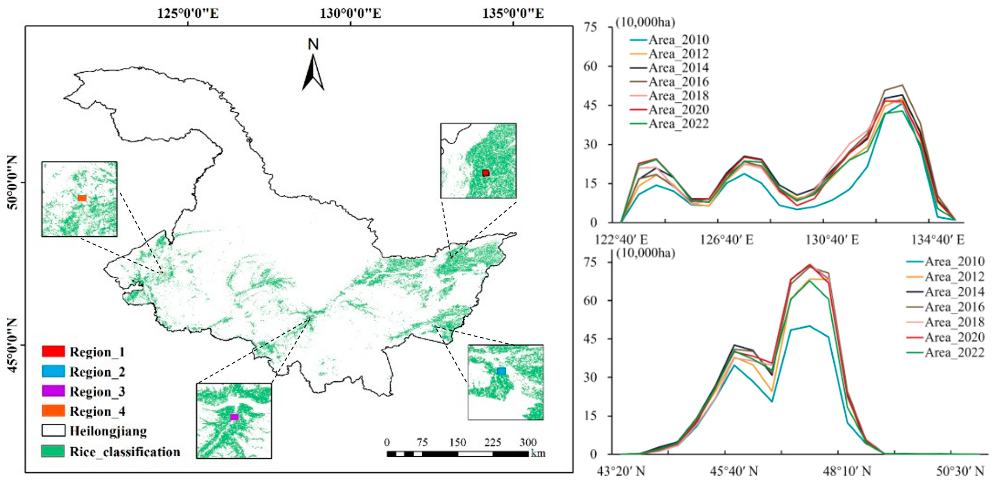
2.1. Study Area

Heilongjiang Province (Figure 1), China (HLJ) was selected as the study area to validate the effectiveness of the proposed method integrating automatic generation of training samples and a machine learning algorithm for rice mapping.

Heilongjiang Province is located in northeastern China, with 12 prefectural-level cities and one region (Daxinganling Region) under its jurisdiction, covering a total area of 473,000 square kilometers. The province spans four major water systems: the Heilongjiang, Ussuri, Songhua, and Suifen rivers. It has a cold-temperate and temperate continental monsoon climate, with an average annual precipitation of 400–800 mm, and the average annual temperature ranges from −4 °C to 6 °C. Crops in the province are mainly single-season crops; the main crops are rice, corn, and soybeans. Rice is usually sown in mid-April, transplanted at the end of May to early June, and harvested at the end of September and in early October. The current study did not include the Daxinganling region, due to the lack of suitable conditions for agricultural cultivation in the region.

2.2. Data

2.2.1. Landsat Data

In this study, we used Landsat-7 and Landsat-8 images from 2010–2022, featuring large similarities in the visible and near-infrared spectral ranges, with a spatial resolution of 30 m and a temporal resolution of 16 days, together providing a revisit cycle of 8 days. The Scan Lines Corrector (SLC) of Landsat-7 has suffered a mechanical failure since 2003, resulting in data overlap and loss of about 25% of the data in the acquired images; the data can only be corrected using the SLC-off model. To address these problems, this study focused on the preprocessing of Landsat-7 by means of the C Function of Masking (CF-Mask) algorithm [38] and the exclusion of pixels larger than 0.2 in the blue band. Landsat-8 has been in operation since 2013 and carries the Operational Land Imager, which uses a panchromatic band with a narrower range, enabling for better differentiation between vegetated and non-vegetated features in panchromatic imagery.

The distribution of rice fields in Northeast China is relatively stable [39]. In order to overcome the problem of cloud occlusion, in this study, we used three years as the time span, combining each year’s image with the adjacent upper and lower two years’ images to generate a composite image containing rich climatic information. Based on the characteristics of rice growth in the study area [24], Landsat images of four key phenological periods for rice (bare soil, transplanting, growth, and maturity) were selected. All the data were processed on GEE due to the huge volumes of data involved.

2.2.2. Categorized Data on Agricultural Land Use

The China Land Cover Dataset (CLCD) [40] was published by Prof. Xin Huang of Wuhan University, based on 335,709 views of Landsat data and produced on the Google Earth Engine, containing year-by-year land cover information for China. In this study, the CLCD dataset was used for masking non-rice areas; previous studies [39,40] have shown that this method can improve the accuracy of the extracted data.

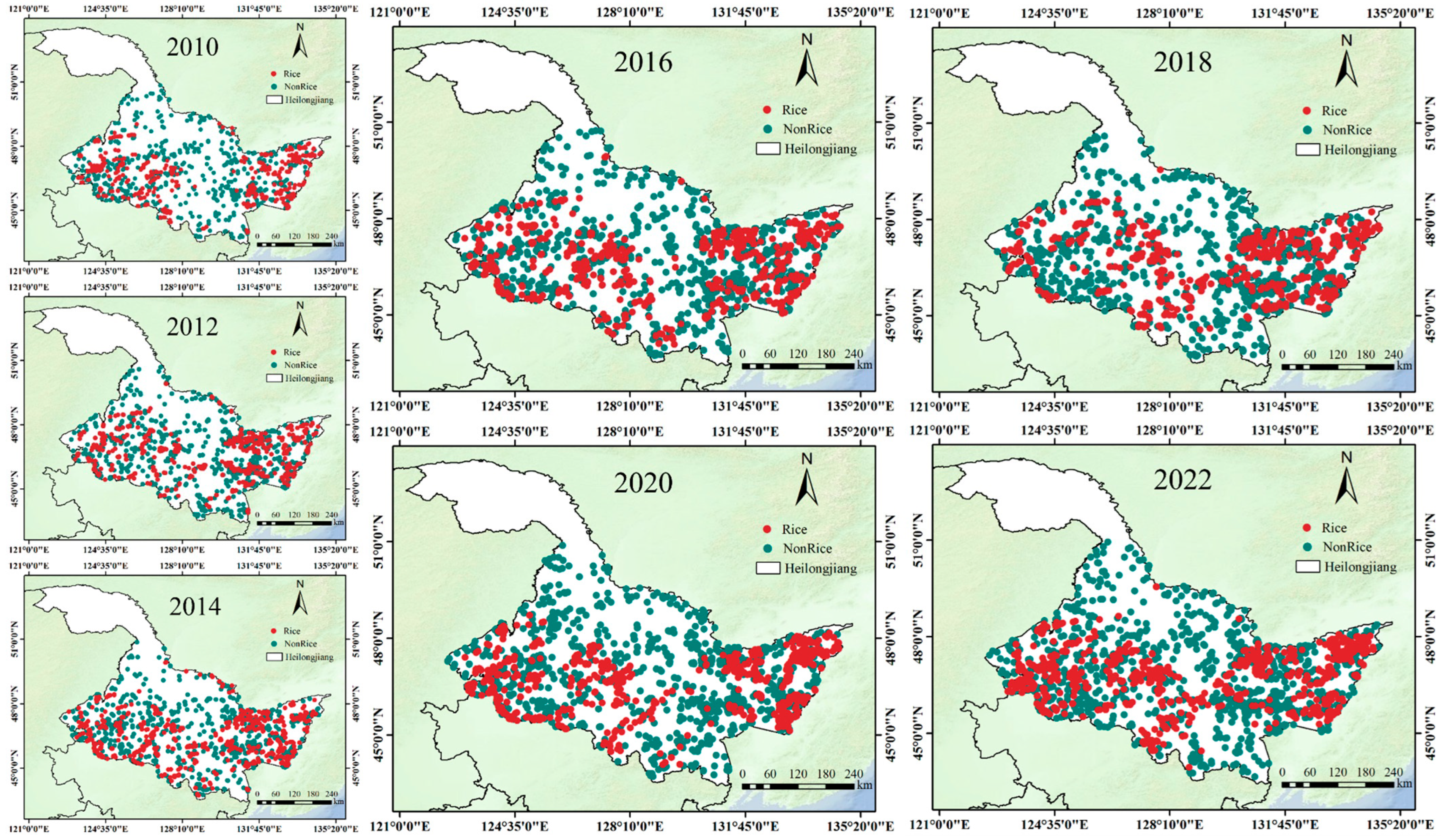
2.2.3. Automatically Generated Ground Sample Data

The overall area of HLJ is large, and for this study, it was divided according to 12 prefecture-level cities. Each prefecture-level city was further divided into 16 equal-sized grids, and rice and non-rice sample points were extracted from each grid to finally summarize all the sample points. This method ensured the reliability of the generated samples while controlling the spatial autocorrelation to some extent. The spatial distribution of the extracted sample points is shown in Figure 2 and was visually evaluated using Landsat images, Sentinel-2 images, and Google images. Finally, the distributional accuracy was assessed by calculating the overall accuracy (OA) and Kappa coefficient.

2.2.4. Agricultural Statistics

Based on the statistical yearbooks of Heilongjiang Province for previous years, the official agricultural statistics of Heilongjiang Province from 2010 to 2022 were collected to validate the accuracy of the LR algorithm in extracting the rice area data.

2.2.5. Existing Rice Mapping Products

In this study, published rice mapping products were collected and compared with the rice distribution maps generated by the LR algorithm, to evaluate the performance of the different algorithms. The CLCD currently contains year-by-year land cover information for China at 30 m resolution for the years 1985 and 1990–2022. Each year’s CLCD dataset is based on all the available Landsat data on GEE. Spatio-temporal features were analyzed, and the classification results were obtained by combining RF classifiers. A post-processing method that included spatio-temporal filtering and logical inference has been proposed to further improve the spatio-temporal consistency of the CLCD (“CLCD_Rice”). Han et al. used multisource remotely sensed data [17] to generate the 2000–2020 spatial and temporal trends of annual rice cultivation area and cultivation intensity across the Asian monsoon region at 500 m resolution (“Han_Rice”). Xuan et al. utilized Landsat-8 time-series imagery from 2013–2021 [41] and a hexagonal auto-sampling method with an RF algorithm (“Xuan_Rice”) to generate a 30 m resolution rice distribution map of Northeast China. Zhang et al. proposed a flexible phenological supervised rice (PSPR) mapping framework using GEE [5], generating a 30 m resolution rice map from 1990 to 2020 (with an interval of five years) for Heilongjiang Province, China (“PSPR _Rice”).

3. Research Methodology

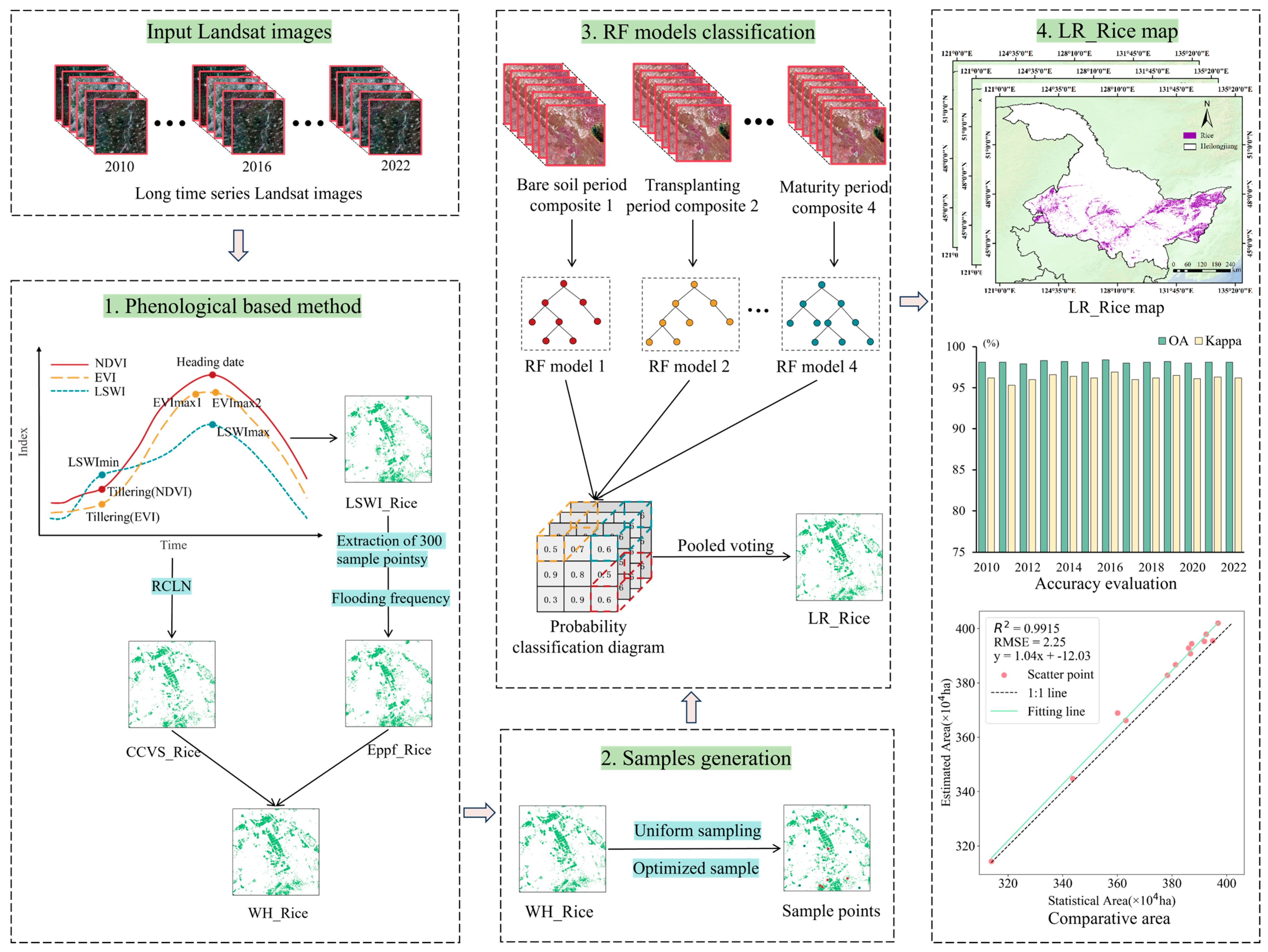
3.1. Introduction to Research Methods

In this study, a rice mapping method integrating climatology-assisted automatic generation of training samples and machine learning algorithms is proposed, as shown in Figure 3. The method first generates a preliminary rice distribution map based on phenology and selects 300 sample points per year from the Landsat imagery, Google imagery, and CLCD datasets, respectively, for element recognition in rice images via the Eppf-CM method. Subsequently, F and RCLN were introduced to recognize rice image elements using the CCVS method. The potential rice distribution map (“WH_Rice”) was generated by combining the intersecting rice image elements identified by the Eppf-CM and CCVS methods, and the grid was then divided for uniform sampling to automatically generate evenly distributed rice/non-rice training sample. Representative samples were purified by extracting the neighboring information via an alternating iteration method, which is further described in Section 3.3, below. Finally, the optimized sample data were synthesized into stage data based on the four key phenological periods, respectively, and the machine learning model was trained on each phenological period to generate multiple rice-probability classification maps. The final extracted rice maps were drawn using the pooled voting strategy, and finally, the OA and Kappa coefficients were computed to evaluate the accuracy.

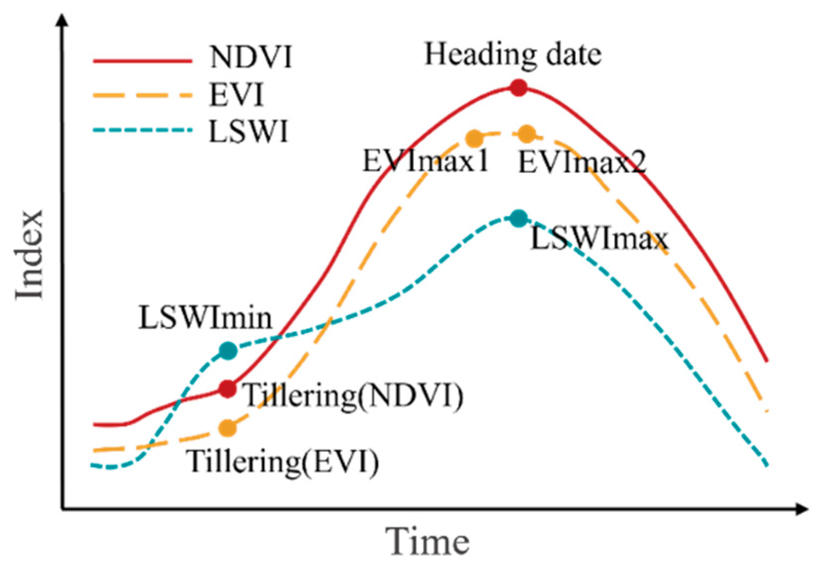
3.2. Mapping the Potential Distribution of Rice Based on Phenology

The LSWI method proposed by Xiao et al. [6] has been widely used in rice mapping, and this study was based on the use of th LSWI method to generate a preliminary rice distribution map. The main idea of the LSWI-based rice classification algorithm is that the value of the LSWI is than the NDVI during the transplanting stage, and the value of the LSWI is smaller than NDVI during the growing stage. Therefore, the following formula was applied to the Landsat image during the transplanting stage to obtain the preliminary rice distribution map, and the preliminary rice distribution map was subsequently compared with the Landsat images, Google images, and CLCD dataset for each year, and 300 sample points were extracted for each year for the subsequent Eppf-CM method to identify the image elements.

$$R{\mathrm{ice}}_{LSWI}=\left\{\begin{array}{c}1,LSWI-NDVI\ge T_0\\ 0,LSWI-NDVI<T_0\end{array}\right.$$

(1)

$$NDVI={\displaystyle \frac{{\rho }_{NIR}-{\rho }_{RED}}{{\rho }_{NIR}+{\rho }_{RED}}}$$

(2)

$$LSWI={\displaystyle \frac{{\rho }_{NIR}-{\rho }_{SWIR}}{{\rho }_{NIR}+{\rho }_{SWIR}}}$$

(3)

where ${\rho }_{NIR}$, ${\rho }_{SWIR}$, and ${\rho }_{RED}$ denote the near-infrared, short-wave infrared, and red light bands, respectively, $R{\mathrm{ice}}_{LSWI}$ is the rice information detected by the $LSWI$, 1 and 0 denote rice and non-rice, respectively, and $T_0$ is set to 0 with reference to previous studies [6,23].

The Eppf-CM method proposed by Ni et al. [24] and the CCVS method developed by Qiu et al. [11] perform well in rice mapping, with high accuracy. To reduce the uncertainty inherent in these two methods, this study combined them to generate potential rice distribution maps.

The Eppf-CM method constructed a new feature set based on four key phenological periods of rice: bare soil stage (75–120 days), transplanting stage (130–170 days), growing stage (180–250 days), and maturity stage (270–300 days), including Bare Soil Index (BSI) for bare soil stage, LSWI and Green Chlorophyll Vegetation Index (GCVI) during the growing period, NDVI and Enhanced Vegetation Index (EVI) during the growing period, and Plant Senescence Reflectance Index (PSRI) during the maturity period. The index images for each season were constructed by the median synthesis method in GEE, and the corresponding synthetic feature images were generated. The synthetic feature images and the selected 300 sample points were input to a one-class classifier (OCSVM) to generate the rice distribution map “$R{\mathrm{ice}}_{Eppf-CM}$”.

Considering the green vegetation characteristic of the late growth stage in rice, the maximum NDVI value for this stage was synthesized to further identify the green rice plants and reduce the effects of cloud shading and striping of the Landsat-7 images. The formula is as follows:

$$NDV{I}_{\max }=\max (NDV{I}_{T_1},NDV{I}_{T_2},\cdots ,NDV{I}_{T_n})$$

(4)

$$R\mathrm{ice}1=\left\{\begin{array}{cc}1,\hfill & \hfill R{\mathrm{ice}}_{Eppf-CM}=1 \mathrm{and} NDV{I}_{\max }\ge T_{NDVI}\\ 0,\hfill & \hfill Others\end{array}\right.$$

(5)

where $NDV{I}_{T_i}$ denotes the NDVI image data acquired at the moment of $T_i$, n is the maximum number of images in each region, $\max ()$ denotes the maximum value in the corresponding time-series data for each pixel, $NDV{I}_{\max }$ is the maximum value synthesized by NDVI, $R\mathrm{ice}1$ denotes the rice pixel screened by combining Eppf-CM and $NDV{I}_{\max }$, and $T_{NDVI}$ is set to 0.7 according to a previous study [36].

There is variability in the climate and environment in different regions, and rice phenology changes accordingly, so the confidence level of rice extraction using phenological methods may be biased. F represents the frequency of flooding, the total number of times the rice signal was detected during the rice transplanting phase divided by the number of all high-quality images of that pixel throughout the rice transplanting phase. Introducing F into the climatology-assisted rice mapping task results in rice distribution maps with higher confidence. Considering that the revisit period of Landsat images is 16 days and the vast majority of areas have two or three views of image data available, the value interval of F was set to [0.3, 0.6]. The specific calculation formula is as follows:

$$F={\displaystyle \frac{\sum N_{flood}}{\sum N_{total}}}$$

(6)

$$R\mathrm{ice}2=\left\{\begin{array}{cc}1,\hfill & \hfill R\mathrm{ice}1=1 \mathrm{and} 0.3<F<0.6\\ 0,\hfill & \hfill Others\end{array}\right.$$

(7)

where $F$ denotes the flooding frequency of each pixel, $\sum N_{flood}$ is the total number of rice signals detected by the LSWI weathering method, $\sum N_{total}$ is the total number of high-quality observed images for each pixel, and $R\mathrm{ice}2$ is the rice pixels that are further filtered based on $R\mathrm{ice}1$ and $F$.

The main basis of the CCVS rice mapping method is that from tillering to the tasseling stage, the magnitude of change in LSWI in rice fields is relatively small and increases in the Enhanced Vegetation Index2 (EVI2) are significant. Therefore, the ratio of the amplitude of change in LSWI and EVI2 from tillering to spiking (RCLE) can be used as the main index for extracting rice data; the smaller the value of RCLE, the higher the probability of being categorized as rice. Meanwhile, the minimum LSWI value of rice is higher than that of other non-hydroponic crops during the transplanting period. As shown in Figure 4, both the NDVI and EVI values of rice increased significantly from the transplanting stage to the tasseling stage. A pseudo-peak (EVImax1) appeared in the EVI value before it reached the true peak (EVImax2), whereas there was only one peak in the NDVI, which expressed a more pronounced magnitude of change. Therefore, in this study, the EVI2 index in the RCLE was replaced by the NDVI index, which became the ratio of the amplitude of change in LSWI to NDVI (abbreviated as RCLN). The formula for RCLN is as follows:

$$RCLN={\displaystyle \frac{LSW{I}_{heading}-LSW{I}_{transplanting}}{NDV{I}_{heading}-NDV{I}_{transplanting}}}$$

(8)

where $LSW{I}_{heading}$ and $NDV{I}_{heading}$ represent LSWI and NDVI values at the tasseling stage, and $LSW{I}_{transplanting}$ and $NDV{I}_{transplanting}$ represent LSWI and NDVI values at the transplanting stage, respectively.

The formula for CCVS-extracted rice mapping is as follows:

$$R{\mathrm{ice}}_{CCVS}=\left\{\begin{array}{cc}1,\hfill & \hfill LSW{I}_{\min }>0.1 \mathrm{and} RCLN<0.6\\ 0,\hfill & \hfill Others\end{array}\right.$$

(9)

where $LSW{I}_{\min }$ denotes the minimum value of LSWI during the transplanting period and the threshold value is consistent with Qiu et al. [11], and $R{\mathrm{ice}}_{CCVS}$ denotes the rice pixels detected via the CCVS method.

Subsequently, a preliminary rice distribution map was generated through combining the two methods with the following equation:

$$R{\mathrm{ice}}_{WH}=\left\{\begin{array}{cc}1,\hfill & \hfill Rice2=1 \mathrm{and} Ric{e}_{CCVS}=1\\ 0,\hfill & \hfill Others\end{array}\right.$$

(10)

where $R{\mathrm{ice}}_{WH}$ indicates the map of potential rice distribution “WH_Rice” extracted via the Eppf-CM and CCVS methods.

Finally, in order to minimize rice misclassification, the CLCD dataset was used to apply a non-rice mask on $R{\mathrm{ice}}_{WH}$. Outliers were eliminated, and a final composite phenological rice distribution map was generated.

3.3. Sample Extraction and Optimization

In this paper, the study area was large, and was divided according to prefecture-level cities, with each prefecture-level city then divided according to a grid, and sample points extracted from each grid stratification. Finally, the samples were summarized to realize the automatic generation of rice/non-rice training samples according to WH_Rice. This method ensured the reliability of the generated samples while controlling the spatial autocorrelation to some extent. However, this plain sample generation method may have introduced confusion between rice and non-rice data samples, with an impact on the subsequent classification. Therefore, the current study purified the samples to make them more representative by extracting neighborhood information via an alternating iterative method. After stratified sampling, the statistical features of the sample points were extracted from within a 3 × 3 neighborhood window of each, and the overall intraclass statistical properties were calculated. Then, an alternating iteration strategy was used to optimize the sample set, as follows. For a fixed category (e.g., rice), calculate its similarity with other categories (e.g., non-rice), and eliminate the confusing sample points to obtain a purer subset; then, perform the same operation for another category to optimize its samples. Through several iterations, a more reliable and representative training sample set is finally obtained.

3.4. Integrated Monthly RF Modeling

RF has been widely used in rice mapping research, due to the ease of use of the RF model on the GEE platform, its stable classification performance, and the easy calculation of classification probability [29,42]. Due to problems with cloud masking and SLC-off stripes in Landsat-7 images, the large number of randomly distributed null values mean that the extracted rice distribution maps would also include null regions with incomplete mapping results when classified purely using the RF model. In order to solve this problem, this study considered three years as the time span, combining the images from each year with images from the preceding and subsequent years. The proposed integrated classification model of sub-climatic RF probability for the four key rice seasons directly classifies the synthetic image data of a specific time-phase and outputs the categorization probability for each pixel, then combining the probabilities to produce the classification maps integrating multiple synthetic images. This “parallel” organization makes the classification results of each key season independent of each other, which effectively solves the null problem. Therefore, in this study, the optimized sample data were divided into climatic synthetic phases. The binary classification RF models were trained independently to generate multiple probability classification maps, and the final rice maps were drawn using an aggregate voting strategy. The formulas used are as follows:

$$P_i={\displaystyle \frac{1}{T_i}}\sum _{j=1}^{T_i}{P}_i^j$$

(11)

$$Ric{e}_i=\left\{\begin{array}{ll}1,& P_i\ge T_p\\ 0,& Others\end{array}\right.$$

(12)

where $P_i$ denotes the final classification probability that image element $i$ is in a rice category, $T_i$ is the total number of images used to classify image element $i$, $P_i^j$ is the probability that image element $i$ is classified as rice calculated via the RF model of the image in period $j$, $Ric{e}_i$ denotes the final classification value of image element $i$, with 1 denoting that it is categorized as rice and 0 denoting that it is not rice, and $T_p$ is the classification probability segmentation threshold, with a value of 0.5.

In this paper, sample data from four key climatic periods were synthesized via mean staging. The formulas for each vegetation index are listed in

Table 1. Vegetation index table.

Vegetation Index	Calculation
Normalized Difference Vegetation Index (NDVI)	$NDVI={\displaystyle \frac{{\rho }_{NIR}-{\rho }_{RED}}{{\rho }_{NIR}+{\rho }_{RED}}}$
Land Surface Water Index (LSWI)	$LSWI={\displaystyle \frac{{\rho }_{NIR}-{\rho }_{SWIR}}{{\rho }_{NIR}+{\rho }_{SWIR}}}$
Enhanced Vegetation Index (EVI)	$EVI=2.5\times {\displaystyle \frac{{\rho }_{NIR}-{\rho }_{RED}}{{\rho }_{NIR}+6\times {\rho }_{RED}-7.5\times {\rho }_{BLUE}+1}}$
Enhanced Vegetation Index2 (EVI2)	$EVI2=2.5\times {\displaystyle \frac{{\rho }_{NIR}-{\rho }_{RED}}{{\rho }_{NIR}+2.4\times {\rho }_{RED}+1}}$
Bare Soil Index (BSI)	$BSI={\displaystyle \frac{\left({\rho }_{SWIR}+{\rho }_{RED}\right)-\left({\rho }_{NIR}+{\rho }_{BLUE}\right)}{\left({\rho }_{SWIR}+{\rho }_{RED}\right)+\left({\rho }_{NIR}+{\rho }_{BLUE}\right)}}$
Green Chlorophyll Vegetation Index (GCVI)	$GCVI={\displaystyle \frac{{\rho }_{NIR}}{{\rho }_{RED}}}-1$
Plant Senescence Reflectance Index (PSRI)	$PSRI={\displaystyle \frac{{\rho }_{RED}-{\rho }_{BLUE}}{{\rho }_{NIR}}}$
Normalized Difference Water Index (NDWI)	$NDWI={\displaystyle \frac{{\rho }_{GREEN}-{\rho }_{NIR}}{{\rho }_{GREEN}+{\rho }_{NIR}}}$
Modified Normalized Difference Water Index (MNDWI)	$MNDWI={\displaystyle \frac{{\rho }_{GREEN}-{\rho }_{SWIR1}}{{\rho }_{GREEN}+{\rho }_{SWIR1}}}$

. Subsequently, the feature importance of each phenology period was calculated separately, and then several vegetation indices with the highest ranking were selected as the input features of the RF classification model for these four phenological periods, as shown in

Table 2. Model input features table.

Phenological Stage	Input Features for RF
Bare soil period	BSI
Transplanting period	LSWI, GCVI, NDWI, MNDWI
Growth period	NDVI, EVI, EVI2
Maturity period	PSRI

.

The construction of the RF classifier needs to determine the number of trees to be generated (ntree) and the number of variables used to select the best segmentation of tree growth (nfeature), so that when ntree gradually increases, RF classification performance will gradually improve and become stable. In some studies, ntree is set to 200 and nfeature is set to the square root of the total number of features, which achieves excellent cartographic accuracy. Therefore, the current study used a grid search to fine-tune the hyperparameters of the RF model. After synthesizing classification performance and time efficiency, the ntree and nfeature were set to 200 and the square root of the total features, respectively. The process included dividing 70% of the dataset for each phenology period into training sets and the remaining 30% into test sets, to ensure the generalization ability of the model. The more commonly used K-fold cross-validation (K = 5) was used to evaluate the stability of the RF classification model for each phenological period. In the RF training, the data for each phenological period were randomly divided into K sets, with K-1 of these used for training and the remaining one for verification. The final results were averaged to reduce the influence of randomness on the experiment.

4. Experimental Results and Analysis

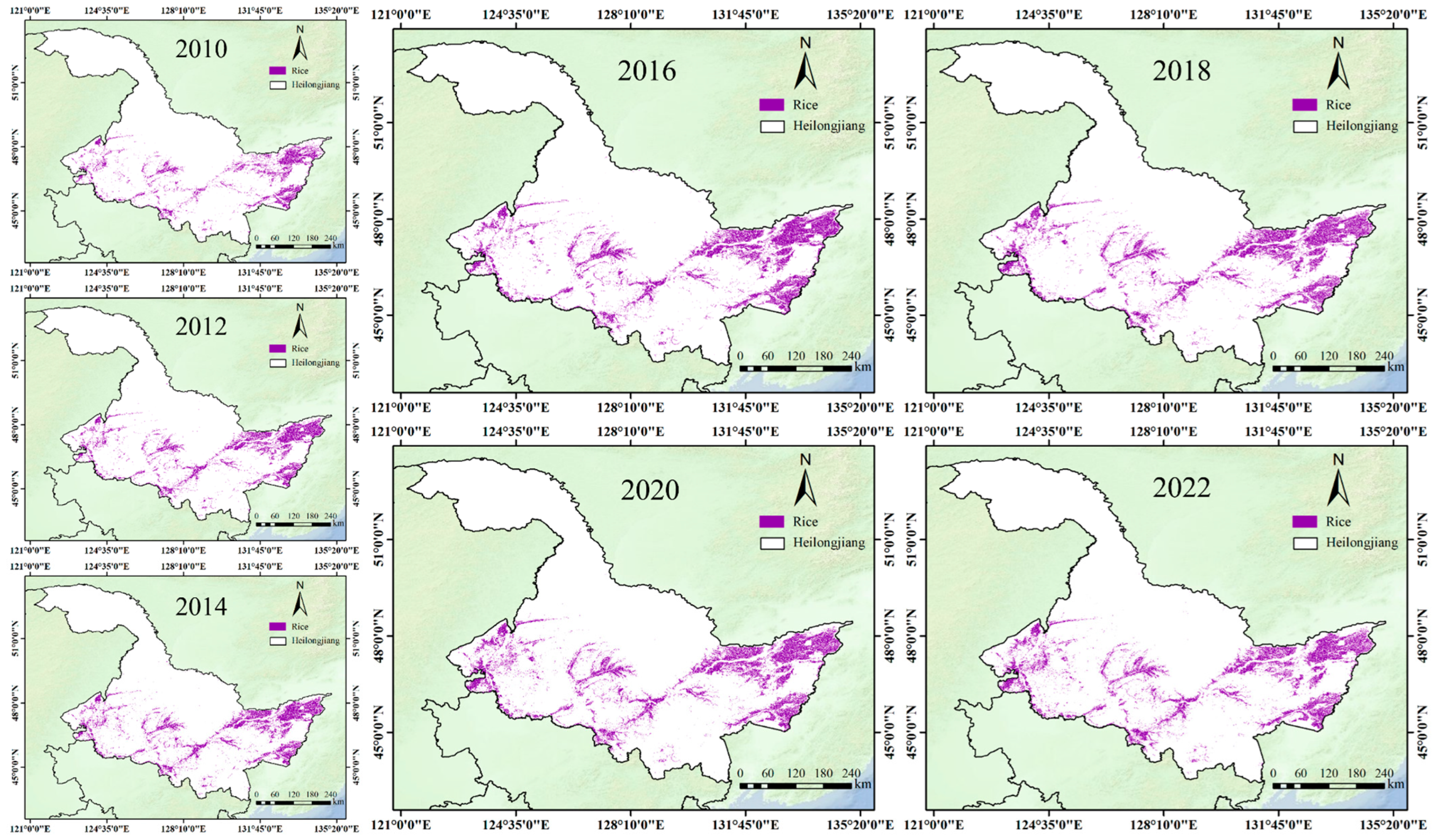
4.1. LR Algorithm for Rice Mapping

Figure 5 shows the distribution of rice at 30 m resolution from 2010 to 2022 in Heilongjiang Province, China (LR_Rice), illustrating that the focus of rice cultivation gradually expanded to the plains on both sides of the river, mainly along the Songhua River on the Nenjiang and Sanjiang plains. With flat terrain, abundant water sources, and a high degree of mechanization, these areas are suitable for large-scale rice cultivation. Subject to the constraints of terrain and available water, rice is mostly distributed in small plots in the form of discrete plots in mountainous areas.

In order to validate the accuracy of the LR-based rice distribution map for HLJ from 2010 to 2022, we calculated a confusion matrix using as an example a visually interpreted ground-referenced real sample and an automatically generated sample. From this matrix, OA and Kappa coefficients were calculated to evaluate the accuracy of LR_Rice, as shown in

Table 3. Confusion matrix of the LR_Rice maps from 2010 to 2022.

Year		Rice	No Rice	PA (%)	UA (%)	F1 (%)	Kappa (%)	OA (%)
2010	Rice	15,316	343	97.5	97.8	97.7	95.5	97.7
	No rice	385	16,278	97.9	97.7
2011	Rice	15,879	421	97.9	97.4	97.7	95.1	97.5
	No rice	342	14,358	97.2	97.7
2012	Rice	13,259	349	98.2	97.4	97.8	95.3	97.7
	No rice	243	11,583	97.1	97.9
2013	Rice	19,542	532	98.1	97.3	97.7	95.2	97.6
	No rice	379	17,366	97	97.9
2014	Rice	13,578	337	98.1	97.6	97.9	95.3	97.7
	No rice	258	11,245	97.1	97.8
2015	Rice	17,246	522	98.5	97.1	97.8	95.2	97.6
	No rice	258	14,578	96.5	98.3
2016	Rice	19,316	529	98.1	97.3	97.7	95.1	97.6
	No rice	379	17,245	97	97.8
2017	Rice	18,659	463	98.2	97.6	97.9	95.3	97.7
	No rice	349	15,249	97.1	97.8
2018	Rice	17,328	432	97.7	97.6	97.6	95.1	97.5
	No rice	403	15,843	97.3	97.5
2019	Rice	22,458	543	98.3	97.6	98	95.3	97.7
	No rice	386	16,847	96.9	97.8
2020	Rice	18,879	496	98.1	97.4	97.8	95.1	97.6
	No rice	358	15,462	96.9	97.7
2021	Rice	21,362	506	97.9	97.7	97.8	95.1	97.6
	No rice	458	17,405	97.2	97.4
2022	Rice	18,724	462	98.3	97.6	97.9	95.3	97.7
	No rice	326	14,279	96.9	97.8

. In the rice classification task results, OA represents the percentage of total pixels that were correctly classified as rice or non-rice. The closer the OA value is to 1, the higher was the overall accuracy of rice classification. Kappa coefficient was used to measure the accuracy and robustness of the model in distinguishing between rice and non-rice pixels. A value closer to 1 means a higher match between the classification results and the real situation, and the better classification performance of the model. The results showed that the accuracy of the rice distribution maps for those thirteen years was relatively stable, with OA values greater than 0.97 and Kappa values greater than 0.95, confirming the LR algorithm’s excellent performance with the HLJ rice mapping data.

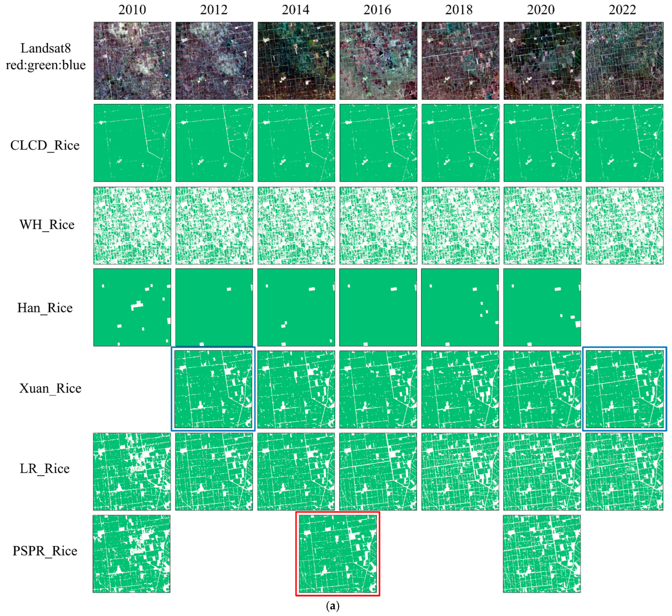
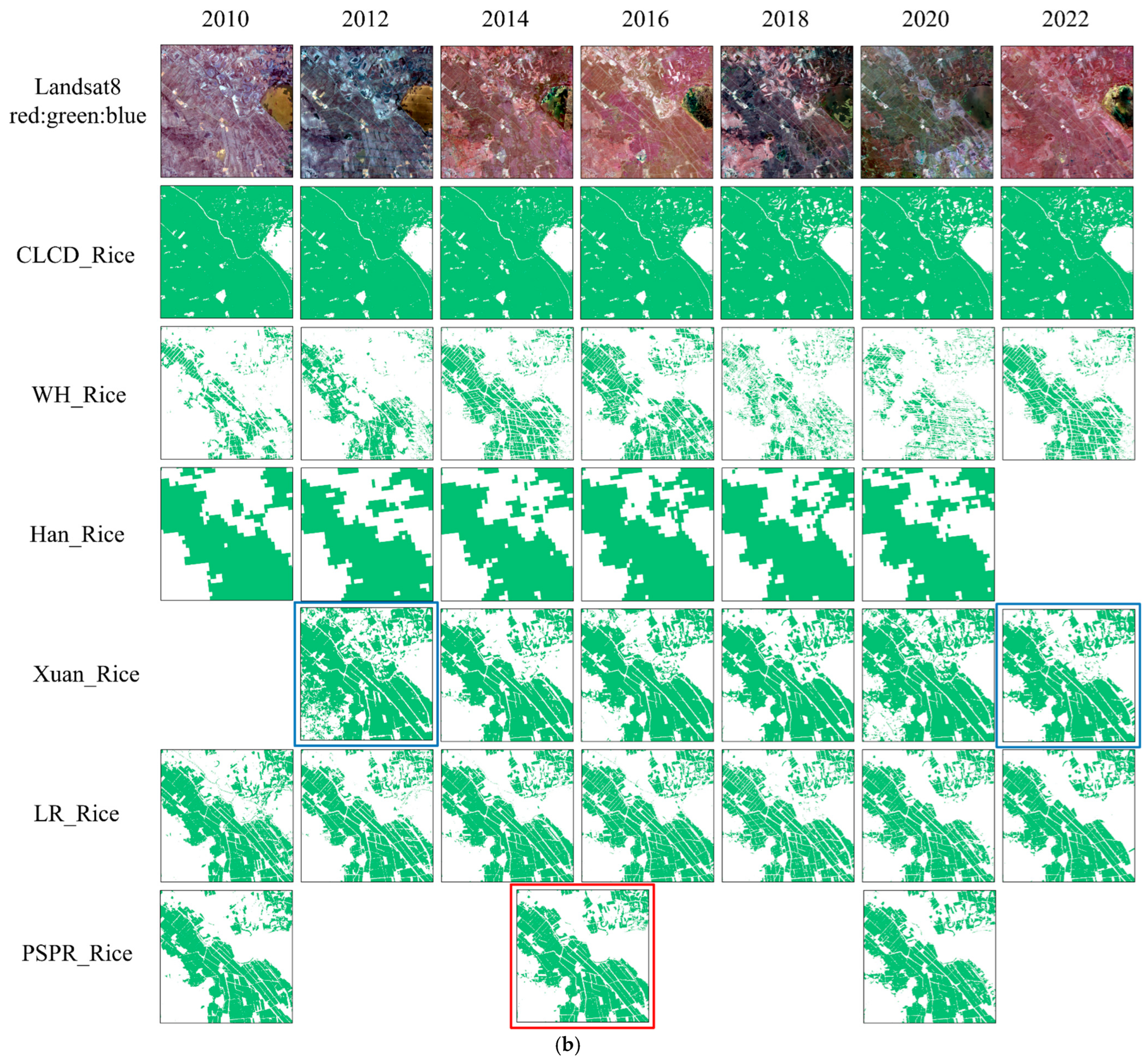
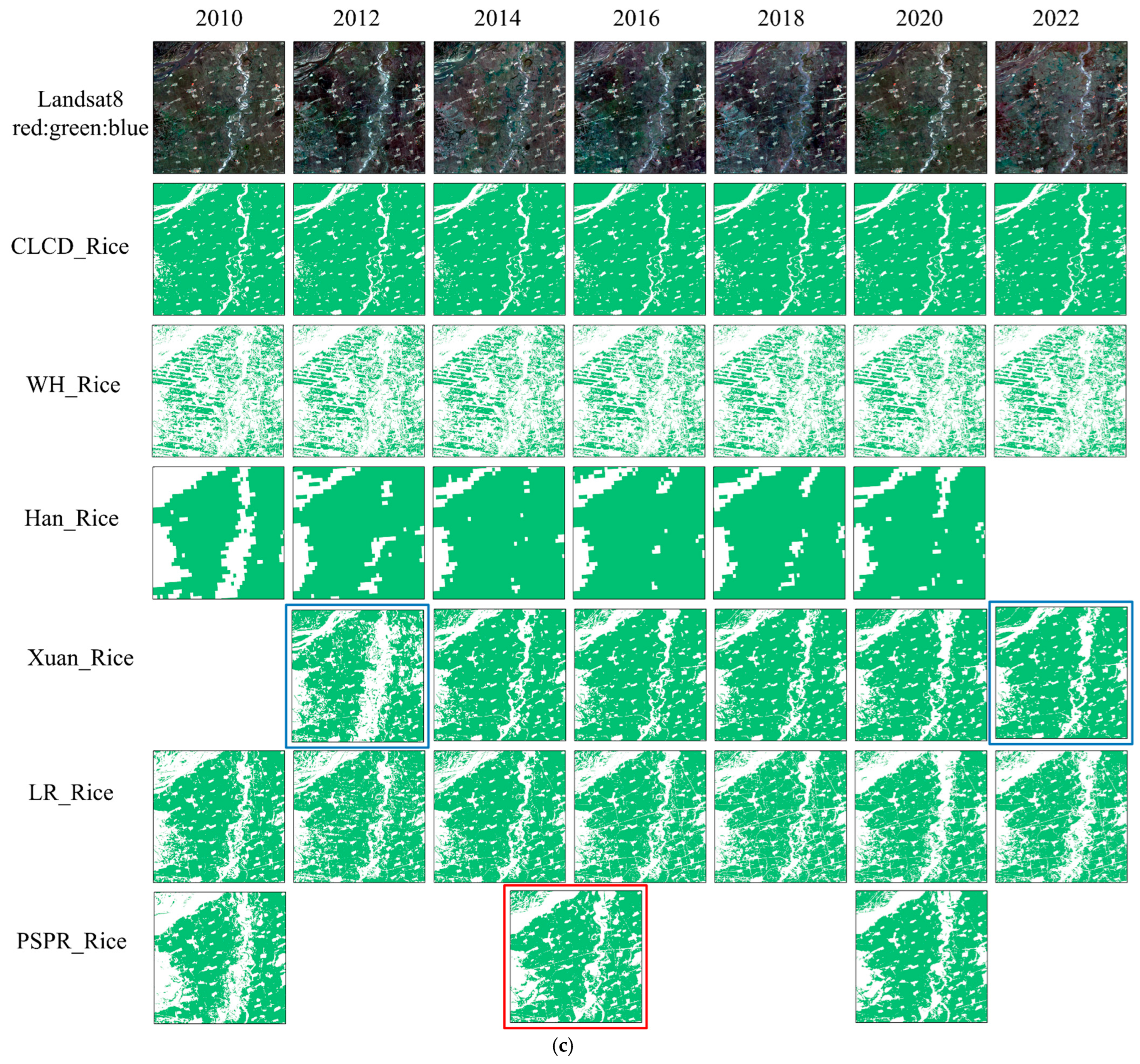
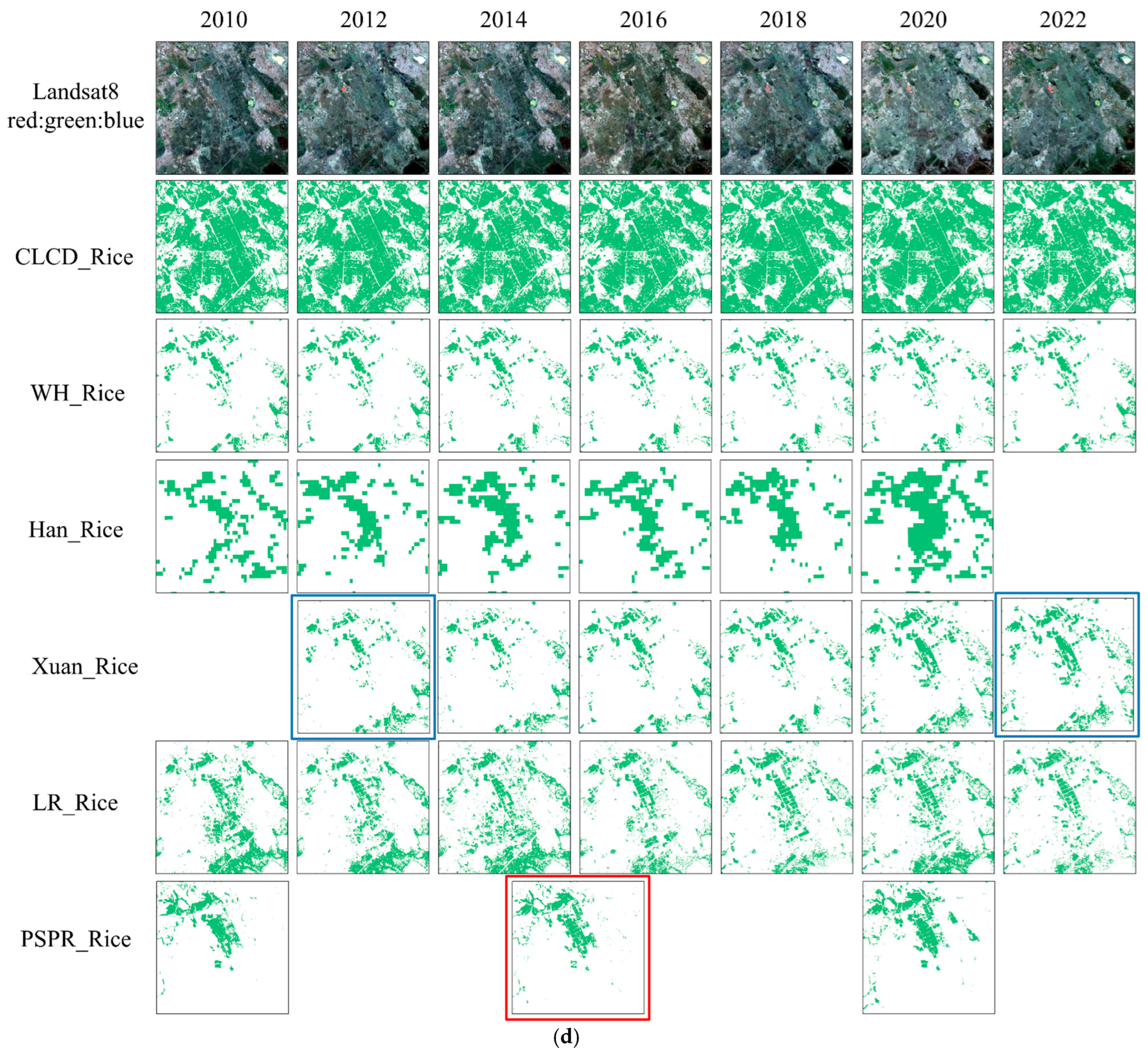
4.2. Comparison with Existing Products and Climatic Maps

In this study, four different regions were selected for comparative analysis of the multi-year rice distribution map extracted by the LR algorithm (LR_Rice) and the four other rice-thematic maps (CLCD_Rice, Han_Rice, Xuan_Rice, PSPR _Rice), as shown in Figure 6, uniformly distributed over the main rice production areas of Heilongjiang Province. The comparison also included a rice distribution map based on HLJ latitude and longitude, which visualized changes in rice area with latitude and longitude. Considering the visual comparison and to verify the reliability of the integrated climatology method, the Landsat optical images and the rice mapping results acquired with the integrated climatology algorithm (WH_Rice) were included in the comparative analysis, as shown in Figure 7.

Figure 7 shows a comparison of LR_Rice with five sets of rice mapping results from four selected sites for 2010–2022 (two-year interval). Since the rice distribution maps for Xuan_Rice have a time frame of 2013–2021 and PSPR _Rice has a time frame of 1990–2020 (five-year interval), and considering that the differences in rice distribution between subsequent years are small, Xuan_Rice 2013 and 2021 were used to fill in 2012 and 2022, respectively; Xuan_Rice’s contributions are labeled with blue boxes, and data from 2015 PSPR _Rice are labeled using red boxes in Figure 7.

Taking the Landsat image as a benchmark, it can be clearly seen that Han_Rice at 500 m includes obvious large misclassification and omission phenomena. CLCD_Rice at 30 m captures the overall rough distribution pattern in a, c, but it makes a lot of omission errors with b, d. WH_Rice at 30 m shows some similarity to LR_Rice, but WH_Rice is affected by cloud occlusion and striping in the early stages, and detailed local features are lost in LR_Rice. WH_Rice is affected by cloud obscuration and striping, losing local detail, and LR_Rice is clearer and more complete.

Comparison of LR_Rice in 2012 and 2022 with Xuan_Rice (labeled in the blue box) confirmed the successful spatial distribution mapping achieved using LR_Rice; the rice field plots showed a very regular structure and shape, and the road information was more complete. In Figure 7, the 2015 PSPR _Rice image marked in the red box is compared with LR_Rice and Xuan_Rice for 2014 and 2016, confirming that PSPR _Rice can better recognize the spatial details of rice than Xuan_Rice, and the extracted information such as water bodies and forest land is more complete. The classification details of LR_Rice across the four regions are more exhaustive, showing higher consistency with the rice distribution in the Landsat images and better overall performance. In summary, the LR algorithm provides higher usability and reliability.

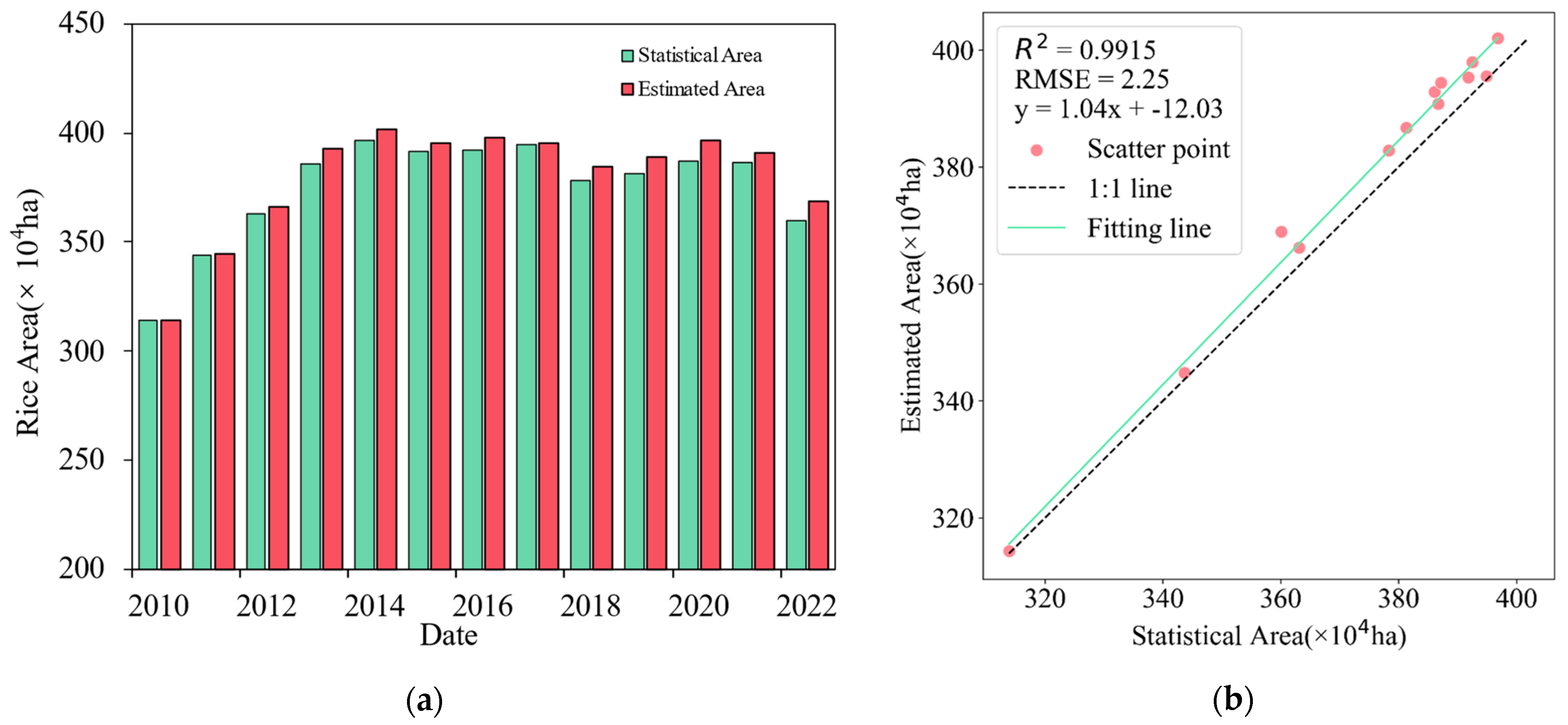
4.3. Comparison of LR Rice Mapping Area with Statistical Area

The obtained agricultural census data were compared with LR to generate maps of the rice area in Heilongjiang Province from 2010 to 2022, and the results are shown in Figure 8. The coefficient of determination R² between the rice area obtained based on LR_Rice and the statistical data was 0.9915, and the RMSE was 22.5 kha, and the two showed an obvious linear relationship, confirming that the agricultural statistics were consistent with and the rice area maps obtained with LR_Rice, reflecting the good classification performance of the LR algorithm.

5. Discussion

5.1. Advantages of the LR Method

Based on the above analysis, the rice distribution map extracted by the LR algorithm had better consistency with the actual rice distribution map, and better classification performance compared with the other methods. The advantages of the LR model are as follows:

(1)

The LR algorithm realizes high-precision rice mapping using Landsat-7 and -8 images from a total of 13 years (2010–2022) of rice distribution mapping in Heilongjiang Province, overcoming the limitation of Sentinel-1/2’s time span, expanding the effective window of data, and effectively mitigating the problems arising from SLC-off image data and cloud occlusion in the Landsat-7 time-series images. This also enables use of Landsat-7 as the main data source for long-time-series rice mapping;

(2)

The LR method generates a preliminary rice distribution map based on the LSWI method. Selecting 300 sample points against the high-resolution image for the Eppf-CM method and introducing F and RCLN for the CCVS method, the potential rice distribution map WH_Rice is generated by combining the Eppf-CM and the CCVS methods. In comparison with the PSPR method that generates a rice distribution map based on phenology, WH_Rice has better consistency with the actual spatial distribution of the rice, indicating that the LR algorithm further improves the quality of the automatically generated sample data and provides favorable data security for the task of extracting rice distribution maps at large scale.

(3)

The study area addressed in this paper was large. When automatically generating sample data for the WH_Rice model, the study area is divided into prefectural cities and then into grids, and the sample points are extracted uniformly grid by grid; then, finally, the samples are summarized. This method not only ensures that the generated samples are more representative but also controls the spatial autocorrelation of the samples to a certain extent.

(4)

The LR algorithm synthesizes stage data for the four key phenological periods, and independently trains the machine learning model to generate multiple rice probability classification maps for each phenological period, adopting the pooled voting strategy to draw the final extracted rice maps, which ensures that the classification results for each phenological period do not interfere with each other in a “concurrent” way, effectively solving the null value problem. This “parallel” approach ensures that the classification results of each season do not interfere with each other and significantly improves the accuracy of rice information extraction.

5.2. Shortcomings and Improvements

In this study, we realized high-precision rice mapping using object-assisted integrated training sample automatic generation and machine learning algorithms, but there is still room for to improve the method’s performance, which we will further explore in the subsequent research. Currently, the following observations should be noted:

(1)

The LR algorithm focuses on extracting single-season rice at high latitudes, while double- or even triple-season rice cropping systems are more common in subtropical and tropical regions. These multi-season rice cropping systems have unique climatic characteristics and can often include multiple flooding and transplanting periods. Therefore, in future studies we will consider optimizing and validating the LR method in multi-season rice growing regions;

(2)

Existing products offering rice mapping of northeast China use data for discrete years and most of them have low resolution. In this study, rice distribution maps with 30 m resolution were generated only for 2010–2022 in HLJ. It is important to extend the analysis timeframe into earlier eras to reveal changes in planting density over longer time scales;

(3)

This study validated the results using existing thematic maps of rice and official statistics, confirming their good spatial coverage and temporal consistency and effectively supporting the assessment of the methodology. Future studies can further enhance the credibility and applicability of the model by introducing more independent validation data;

(4)

In this study, an RF model was used to classify rice, and a number of classification performance indexes were calculated, but there were still shortcomings in the importance analysis of the variables. The lack of detailed analysis of the contribution of each input variable to the classification results, in particular the lack of an “information gain” result ranked by importance of the variables, limited an in-depth understanding of the model’s decision-making mechanism. Furthermore, the nfeatures value of the RF model was not finely optimized, which may have affected the stability and generalization ability of the model.

(5)

Classification errors in this study were mainly concentrated at the junctions of rice and other ground objects, and the classification accuracy of RF model may be unstable in other, more complex scenes. However, although we calculated and provide the confusion matrix, the specific factors leading to false positives (FP) and false negatives (FN) have not been explored in depth; these may relate to environmental conditions or other spatial features. Furthermore, the spatial distribution characteristics of misclassification were not analyzed in depth, which limits our understanding of the causes of classification errors and the development of optimization strategies.

6. Conclusions

In this study, we propose a rice mapping method (LR) using Landsat image data, incorporating automatic generation of training samples and machine learning algorithms, deployed on GEE. The proposed LR method was combined with Eppf-CM and CCVS approaches to realize climate-assisted automated generation of sample data and extract the final rice distribution map. This study mapped 30 m resolution rice distribution data for HLJ from 2010 to 2022, and the accuracy indexes were relatively stable, with OA values greater than 0.97 and Kappa values greater than 0.95. When LR_Rice was analyzed in comparison with other existing rice thematic areas, the results showed that LR_Rice extracted significant spatial distribution characteristics of the rice and more complete information on non-rice. When the rice-planted area extracted by LR_Rice was compared with the agricultural statistics, the coefficient of determination R² was 0.9915, the RMSE was 22.5 kha, and the two displayed a significant linear relationship; the slope of the linear equation was 1.04. The LR algorithm breaks through the bottleneck of medium- and high-resolution optical remote sensing imagery of rice mapping, alleviates the limitation of the lack of data in the long time series of large-scale rice mapping samples. The use of this algorithm in the current study to obtain accurate information on rice cultivation across a large region is of great significance for food security, water resource management, and environmentally sustainable development.

In view of the limitations of this study, future work will include variable importance analysis, quantifying the contribution of each input variable to the model decision using methods such as Gini importance or mean reduction accuracy, integrating soil moisture data or regional soil databases to more comprehensively consider the impact of soil variables on rice classification. In addition, we will combine geographical weighted regression (GWR), spatial error analysis, and multi-temporal remote sensing data to deeply explore the spatial distribution characteristics of misclassification and analyze the influence of different environmental conditions on classification accuracy, in order to optimize classification strategies and improve the stability and adaptability of the model. In terms of model optimization, we will carry out further tuning of hyperparameters, comprehensively analyzing the OOB error curve to determine the optimal value range of nfeatures, exploring the adaptability of parameters and the features of data from different regions to enhance the robustness and generalization ability of the model. These improvements should further improve the reliability and accuracy of the proposed method, aiming to provide more solid technical support for rice mapping research.

References

1. Tornos, L.; Huesca, M.; Antonio Dominguez, J.; Carmen Moyano, M.; Cicuendez, V.; Recuero, L.; Palacios-Orueta, A. Assessment of MODIS Spectral Indices for Determining Rice Paddy Agricultural Practices and Hydroperiod. ISPRS J. Photogramm. Remote Sens. 2015, 101, 110–124. [Google Scholar] [CrossRef]
2. Zhang, G.; Xiao, X.; Dong, J.; Xin, F.; Zhang, Y.; Qin, Y.; Doughty, R.B.; Moore, B. Fingerprint of Rice Paddies in Spatial–Temporal Dynamics of Atmospheric Methane Concentration in Monsoon Asia. Nat. Commun. 2020, 11, 554. [Google Scholar] [CrossRef]
3. Meng, L.; Li, Y.; Shen, R.; Zheng, Y.; Pan, B.; Yuan, W.; Li, J.; Zhuo, L. Large-Scale and High-Resolution Paddy Rice Intensity Mapping Using Downscaling and Phenology-Based Algorithms on Google Earth Engine. Int. J. Appl. Earth Obs. Geoinf. 2024, 128, 103725. [Google Scholar] [CrossRef]
4. Dong, J.; Xiao, X. Evolution of Regional to Global Paddy Rice Mapping Methods: A Review. ISPRS J. Photogramm. Remote Sens. 2016, 119, 214–227. [Google Scholar] [CrossRef]
5. Zhang, C.; Zhang, H.; Tian, S. Phenology-Assisted Supervised Paddy Rice Mapping with the Landsat Imagery on Google Earth Engine: Experiments in Heilongjiang Province of China from 1990 to 2020. Comput. Electron. Agric. 2023, 212, 108105. [Google Scholar] [CrossRef]
6. Xiao, X.; Boles, S.; Liu, J.; Zhuang, D.; Frolking, S.; Li, C.; Salas, W.; Moore, B. Mapping Paddy Rice Agriculture in Southern China Using Multi-Temporal MODIS Images. Remote Sens. Environ. 2005, 95, 480–492. [Google Scholar] [CrossRef]
7. Zhang, X.; Su, H.; Zhang, C.; Gu, X.; Tan, X.; Atkinson, P.M. Robust Unsupervised Small Area Change Detection from SAR Imagery Using Deep Learning. ISPRS J. Photogramm. Remote Sens. 2021, 173, 79–94. [Google Scholar] [CrossRef]
8. Dong, J.; Xiao, X.; Menarguez, M.A.; Zhang, G.; Qin, Y.; Thau, D.; Biradar, C.; Moore, B. Mapping Paddy Rice Planting Area in Northeastern Asia with Landsat 8 Images, Phenology-Based Algorithm and Google Earth Engine. Remote Sens. Environ. 2016, 185, 142–154. [Google Scholar] [CrossRef]
9. Jin, C.; Xiao, X.; Dong, J.; Qin, Y.; Wang, Z. Mapping Paddy Rice Distribution Using Multi-Temporal Landsat Imagery in the Sanjiang Plain, Northeast China. Front. Earth Sci. 2016, 10, 49–62. [Google Scholar] [CrossRef]
10. Belgiu, M.; Bijker, W.; Csillik, O.; Stein, A. Phenology-Based Sample Generation for Supervised Crop Type Classification. Int. J. Appl. Earth Obs. Geoinf. 2021, 95, 102264. [Google Scholar] [CrossRef]
11. Qiu, B.; Li, W.; Tang, Z.; Chen, C.; Qi, W. Mapping Paddy Rice Areas Based on Vegetation Phenology and Surface Moisture Conditions. Ecol. Indic. 2015, 56, 79–86. [Google Scholar] [CrossRef]
12. Shen, R.; Pan, B.; Peng, Q.; Dong, J.; Chen, X.; Zhang, X.; Ye, T.; Huang, J.; Yuan, W. High-Resolution Distribution Maps of Single-Season Rice in China from 2017to 2022. Earth Syst. Sci. Data 2023, 15, 3203–3222. [Google Scholar] [CrossRef]
13. Sun, L.; Lou, Y.; Shi, Q.; Zhang, L. Spatial Domain Transfer: Cross-Regional Paddy Rice Mapping with a Few Samples Based on Sentinel-1 and Sentinel-2 Data on GEE. Int. J. Appl. Earth Obs. Geoinf. 2024, 128, 103762. [Google Scholar] [CrossRef]
14. Xiao, X.; He, L.; Salas, W.; Li, C.; Moore, B.; Zhao, R.; Frolking, S.; Boles, S. Quantitative Relationships between Field-Measured Leaf Area Index and Vegetation Index Derived from VEGETATION Images for Paddy Rice Fields. Int. J. Remote Sens. 2002, 23, 3595–3604. [Google Scholar] [CrossRef]
15. Lin, Z.; Zhong, R.; Xiong, X.; Guo, C.; Xu, J.; Zhu, Y.; Xu, J.; Ying, Y.; Ting, K.C.; Huang, J.; et al. Large-Scale Rice Mapping Using Multi-Task Spatiotemporal Deep Learning and Sentinel-1 SAR Time Series. Remote Sens. 2022, 14, 699. [Google Scholar] [CrossRef]
16. Xiao, X.M.; Boles, S.; Frolking, S.; Li, C.S.; Babu, J.Y.; Salas, W.; Moore, B. Mapping Paddy Rice Agriculture in South and Southeast Asia Using Multi-Temporal MODIS Images. Remote Sens. Environ. 2006, 100, 95–113. [Google Scholar] [CrossRef]
17. Han, J.; Zhang, Z.; Luo, Y.; Cao, J.; Zhang, L.; Zhuang, H.; Cheng, F.; Zhang, J.; Tao, F. Annual Paddy Rice Planting Area and Cropping Intensity Datasets and Their Dynamics in the Asian Monsoon Region from 2000 to 2020. Agric. Syst. 2022, 200, 103437. [Google Scholar] [CrossRef]
18. Zhou, Y.; Xiao, X.; Qin, Y.; Dong, J.; Zhang, G.; Kou, W.; Jin, C.; Wang, J.; Li, X. Mapping Paddy Rice Planting Area in Rice-Wetland Coexistent Areas through Analysis of Landsat 8 OLI and MODIS Images. Int. J. Appl. Earth Obs. Geoinf. 2016, 46, 1–12. [Google Scholar] [CrossRef]
19. Han, J.; Zhang, Z.; Luo, Y.; Cao, J.; Zhang, L.; Cheng, F.; Zhuang, H.; Zhang, J.; Tao, F. NESEA-Rice10: High-Resolution Annual Paddy Rice Maps for Northeast and Southeast Asia from 2017 to 2019. Earth Syst. Sci. Data 2021, 13, 5969–5986. [Google Scholar] [CrossRef]
20. Xiao, W.; Xu, S.; He, T. Mapping Paddy Rice with Sentinel-1/2 and Phenology-, Object-Based Algorithm-A Implementation in Hangjiahu Plain in China Using GEE Platform. Remote Sens. 2021, 13, 990. [Google Scholar] [CrossRef]
21. Wei, J.; Cui, Y.; Luo, W.; Luo, Y. Mapping Paddy Rice Distribution and Cropping Intensity in China from 2014 to 2019 with Landsat Images, Effective Flood Signals, and Google Earth Engine. Remote Sens. 2022, 14, 759. [Google Scholar] [CrossRef]
22. Zhang, K.; Lv, X.; Guo, B.; Chai, H. Unsupervised SAR Image Change Detection Based on Histogram Fitting Error Minimization and Convolutional Neural Network. Remote Sens. 2023, 15, 470. [Google Scholar] [CrossRef]
23. Dong, J.; Xiao, X.; Kou, W.; Qin, Y.; Zhang, G.; Li, L.; Jin, C.; Zhou, Y.; Wang, J.; Biradar, C.; et al. Tracking the Dynamics of Paddy Rice Planting Area in 1986-2010 through Time Series Landsat Images and Phenology-Based Algorithms. Remote Sens. Environ. 2015, 160, 99–113. [Google Scholar] [CrossRef]
24. Ni, R.; Tian, J.; Li, X.; Yin, D.; Li, J.; Gong, H.; Zhang, J.; Zhu, L.; Wu, D. An Enhanced Pixel-Based Phenological Feature for Accurate Paddy Rice Mapping with Sentinel-2 Imagery in Google Earth Engine. ISPRS J. Photogramm. Remote Sens. 2021, 178, 282–296. [Google Scholar] [CrossRef]
25. Cai, Y.; Lin, H.; Zhang, M. Mapping Paddy Rice by the Object-Based Random Forest Method Using Time Series Sentinel-1/Sentinel-2 Data. Adv. Space Res. 2019, 64, 2233–2244. [Google Scholar] [CrossRef]
26. Xiao, D.; Niu, H.; Guo, F.; Zhao, S.; Fan, L. Monitoring Irrigation Dynamics in Paddy Fields Using Spatiotemporal Fusion of Sentinel-2 and MODIS. Agric. Water Manag. 2022, 263, 107409. [Google Scholar] [CrossRef]
27. Pan, B.; Zheng, Y.; Shen, R.; Ye, T.; Zhao, W.; Dong, J.; Ma, H.; Yuan, W. High Resolution Distribution Dataset of Double-Season Paddy Rice in China. Remote Sens. 2021, 13, 4609. [Google Scholar] [CrossRef]
28. Xu, X.; Ji, X.; Jiang, J.; Yao, X.; Tian, Y.; Zhu, Y.; Cao, W.; Cao, Q.; Yang, H.; Shi, Z.; et al. Evaluation of One-Class Support Vector Classification for Mapping the Paddy Rice Planting Area in Jiangsu Province of China from Landsat 8 OLI Imagery. Remote Sens. 2018, 10, 546. [Google Scholar] [CrossRef]
29. Chen, C.-F.; Chen, C.-R.; Nguyen-Thanh, S. Investigating Rice Cropping Practices and Growing Areas from MODIS Data Using Empirical Mode Decomposition and Support Vector Machines. GISci. Remote Sens. 2012, 49, 117–138. [Google Scholar] [CrossRef]
30. Zhang, M.; Lin, H.; Wang, G.; Sun, H.; Fu, J. Mapping Paddy Rice Using a Convolutional Neural Network (CNN) with Landsat 8 Datasets in the Dongting Lake Area, China. Remote Sens. 2018, 10, 1840. [Google Scholar] [CrossRef]
31. Clauss, K.; Yan, H.; Kuenzer, C. Mapping Paddy Rice in China in 2002, 2005, 2010 and 2014 with MODIS Time Series. Remote Sens. 2016, 8, 434. [Google Scholar] [CrossRef]
32. Onojeghuo, A.O.; Blackburn, G.A.; Wang, Q.; Atkinson, P.M.; Kindred, D.; Miao, Y. Mapping Paddy Rice Fields by Applying Machine Learning Algorithms to Multi-Temporal Sentinel-1A and Landsat Data. Int. J. Remote Sens. 2018, 39, 1042–1067. [Google Scholar] [CrossRef]
33. Zhang, C.; Zhang, H.; Zhang, L. Spatial Domain Bridge Transfer: An Automated Paddy Rice Mapping Method with No Training Data Required and Decreased Image Inputs for the Large Cloudy Area. Comput. Electron. Agric. 2021, 181, 105978. [Google Scholar] [CrossRef]
34. Sun, Y.; Huang, J.; Ao, Z.; Lao, D.; Xin, Q. Deep Learning Approaches for the Mapping of Tree Species Diversity in a Tropical Wetland Using Airborne LiDAR and High-Spatial-Resolution Remote Sensing Images. Forests 2019, 10, 1047. [Google Scholar] [CrossRef]
35. Teluguntla, P.; Thenkabail, P.S.; Oliphant, A.; Xiong, J.; Gumma, M.K.; Congalton, R.G.; Yadav, K.; Huete, A. A 30-m Landsat-Derived Cropland Extent Product of Australia and China Using Random Forest Machine Learning Algorithm on Google Earth Engine Cloud Computing Platform. ISPRS J. Photogramm. Remote Sens. 2018, 144, 325–340. [Google Scholar] [CrossRef]
36. Chen, N.; Yu, L.; Zhang, X.; Shen, Y.; Zeng, L.; Hu, Q.; Niyogi, D. Mapping Paddy Rice Fields by Combining Multi-Temporal Vegetation Index and Synthetic Aperture Radar Remote Sensing Data Using Google Earth Engine Machine Learning Platform. Remote Sens. 2020, 12, 2992. [Google Scholar] [CrossRef]
37. Kluger, D.M.; Wang, S.; Lobell, D.B. Two Shifts for Crop Mapping: Leveraging Aggregate Crop Statistics to Improve Satellite-Based Maps in New Regions. Remote Sens. Environ. 2021, 262, 112488. [Google Scholar] [CrossRef]
38. Foga, S.; Scaramuzza, P.L.; Guo, S.; Zhu, Z.; Dilley, R.D.; Beckmann, T.; Schmidt, G.L.; Dwyer, J.L.; Hughes, M.J.; Laue, B. Cloud Detection Algorithm Comparison and Validation for Operational Landsat Data Products. Remote Sens. Environ. 2017, 194, 379–390. [Google Scholar] [CrossRef]
39. You, N.; Dong, J.; Huang, J.; Du, G.; Zhang, G.; He, Y.; Yang, T.; Di, Y.; Xiao, X. The 10-m Crop Type Maps in Northeast China during 2017–2019. Sci. Data 2021, 8, 41. [Google Scholar] [CrossRef]
40. Yang, J.; Huang, X. The 30 m Annual Land Cover Dataset and Its Dynamics in China from 1990 to 2019. Earth Syst. Sci. Data 2021, 13, 3907–3925. [Google Scholar] [CrossRef]
41. Xuan, F.; Dong, Y.; Li, J.; Li, X.; Su, W.; Huang, X.; Huang, J.; Xie, Z.; Li, Z.; Liu, H.; et al. Mapping Crop Type in Northeast China during 2013–2021 Using Automatic Sampling and Tile-Based Image Classification. Int. J. Appl. Earth Obs. Geoinf. 2023, 117, 103178. [Google Scholar] [CrossRef]
42. Liu, Y.; Xiao, D.; Yang, W. An Algorithm for Early Rice Area Mapping from Satellite Remote Sensing Data in Southwestern Guangdong in China Based on Feature Optimization and Random Forest. Ecol. Inform. 2022, 72, 101853. [Google Scholar] [CrossRef]
Figure 1. Map of the study area.
Agronomy 15 00873 g001
Figure 2. Distribution map of HLJ rice and non-rice samples.
Agronomy 15 00873 g002
Figure 3. Framework of the proposed LR method.
Agronomy 15 00873 g003
Figure 4. Map of changes in rice vegetation index.
Agronomy 15 00873 g004
Figure 5. Map of rice distribution of rice in HLJ from 2010 to 2022 generated by the LR algorithm.
Agronomy 15 00873 g005
Figure 6. Map of rice area distribution in four selected regions; latitudes and longitudes.
Agronomy 15 00873 g006
Figure 7. Comparison of LR_Rice with five rice mapping results from four selected sites ((a) region 1; (b) region 2; (c) region 3; (d) region 4); a blank space indicates that no data are available for that year.
Agronomy 15 00873 g007aAgronomy 15 00873 g007bAgronomy 15 00873 g007cAgronomy 15 00873 g007d
Figure 8. LR_Rice mapping area and agricultural statistics (a); comparison of the two (b).
Agronomy 15 00873 g008