Bayesian Ensemble Model with Detection of Potential Misclassification of Wax Bloom in Blueberry Images

Abstract

Identifying blueberry characteristics such as the wax bloom is an important task that not only helps in phenotyping (for novel variety development) but also in classifying berries better suited for commercialization. Deep learning techniques for image analysis have long demonstrated their capability for solving image classification problems. However, they usually rely on large architectures that could be difficult to implement in the field due to high computational needs. This paper presents a small (only 1502 parameters) Bayesian–CNN ensemble architecture that can be implemented in any small electronic device and is able to classify wax bloom content in images. The Bayesian model was implemented using Keras image libraries and consists of only two convolutional layers (eight and four filters, respectively) and a dense layer. It includes a statistical module with two metrics that combines the results of the Bayesian ensemble to detect potential misclassifications. The first metric is based on the Euclidean distance (${\mathcal{L}}_2$) between Gaussian mixture models while the second metric is based on a quantile analysis of the binary class predictions. Both metrics attempt to establish whether the model was able to find a good prediction or not. Three experiments were performed: first, the Bayesian–CNN ensemble model was compared with state-of-the-art small architectures. In experiment 2, the metrics for detecting potential misclassifications were evaluated and compared with similar techniques derived from the literature. Experiment 3 reports results while using cross validation and compares performance considering the trade-off between accuracy and the number of samples considered as potentially misclassified (not classified). Both metrics show a competitive performance compared to the state of the art and are able to improve the accuracy of a Bayesian–CNN ensemble model from $96.98\%$ to $98.72\pm 0.54\%$ and $98.38\pm 0.34\%$ for the ${\mathcal{L}}_2$ and $r^2$ metrics, respectively.

1. Introduction

Blueberries (Vaccinium corymbosum L.) are a globally important crop due to their desirable characteristics, such as high phytonutrient content (superfood) [1], and are cultivated globally as an export crop [2]. The exportation of fruits involves a large number of chemical and aesthetic characteristics that must be met in order to be accepted [3]. Failure to reach these can mean either a reduction in price or the complete inability to sell, causing a complete loss [4,5]. Blueberries [6] possess a blue to blue–black epidermis that is covered by a waxy layer or wax bloom, which has been shown to be important for the preservation of quality in blueberries [7,8,9]. This extension of shelf-life is particularly relevant for international shipping to foreign markets, especially from the southern hemisphere to Europe, North America, and China [2]. For this reason, it is important to select berries with a high wax bloom content for export.

Considerable work has been carried out on the application of machine learning and deep learning to agriculture. Such techniques have improved greatly over the last two decades and have reported exceptional results for a wide range of problems such as crop detection, fruit classification [10,11,12], maturity estimation [13,14], fruit counting [15,16], disease diagnosis [17], and automated phenotyping [18,19], among others [20,21,22,23,24,25,26,27,28,29,30,31]. Blueberry cultivars in particular have been well studied using deep learning techniques. Some of the tasks addressed include object detection [32,33], image classification [34], and segmentation [35,36,37].

Quiroz et al. [32] explored the use of deep learning for image recognition of legacy blueberries in the rooting stage. Gonzalez et al. [37] used high-definition images captured in the wild with a mobile device to train a blueberry detection and segmentation model while Ni et al. [36,38] applied segmentation to count berries, to measure maturity, and to evaluate compactness (cluster tightness) automatically.

Maturity estimation for blueberries has been explored by Tan et al. [39] using standard machine learning algorithms such as KNN (K-nearest neighbor) and template matching. MacEachern et al. [40] recently implemented six models to detect blueberries in the wild and to estimate their ripeness. Work in identifying blueberry varieties [41] and yield estimation in blueberry cultivars has also been proposed [42]. All these applications, along with water stress [43] or weed detection in cultivars [44], help to improve blueberry production management. Other machine learning applications for blueberries include attempts to understand after-harvest quality and to develop machinery for automatic sorting [45,46,47]. Zhang et al. [35], for instance, proposed a method based on fully convolutional networks (FCNs) to accurately detect internal bruising in blueberries after mechanical damage.

Fruit characteristics are used to monitor berry development and to improve crop management. Fruit wax bloom is an essential characteristic because consumers consider fruit wax bloom to be an indicator of the freshness of the produce, so consumers prefer fruits with an almost intact waxy layer. Also, Loypimai et al. [9] studied the relation between wax bloom content and postharvest weight loss by the fruit, comparing natural blueberries having a bloom with blueberries rubbed by hand to eliminate the wax bloom, demonstrating that weight loss was more significant from rubbed than unrubbed fruits.

Similarly, Chue et al. [8] studied the effects of wax bloom removal on postharvest blueberry quality, finding that natural bloom removal not only accelerated water loss and decay but also reduced other sensory and nutritional qualities. A lack of bloom decreased the shelf-life, antioxidant concentration, and accelerated accumulation of reactive oxygen species, causing lipid peroxidation and disruption of the organellar membrane structure.

The quantity and uniformity of wax bloom deposition in blueberry fruit at harvest time are genetically determined and, most importantly, the wax bloom may be partially removed during harvest as blueberries are hand-picked and later subject to intensive manipulation during selection and packing [48]. Therefore, selecting berries according to the presence of a wax bloom on the fruit may improve the economic return of blueberries during commercialization. Also, this character is a selection factor in genetic improvement programs, but, up to now, screening is performed using an arbitrary 1-to-5 scale. Designing an automatic and precise method to quantify the presence of wax bloom is a necessity, both to be used during the selection process in the packing house and for use by breeders during the screening of segregants in a breeding program.

When performing such a selection, algorithm robustness is important. Utilizing an algorithm that indicates whether the model is sure about its prediction is desirable. If the prediction is not within a specific range, it would be better to process such berries manually as is presently carried out. Thus, it is better to classify a smaller quantity of berries than make a mistake in the prediction. Misclassification may cause blueberry deterioration (for the lack of bloom) and affect all other berries in the same package.

Bayesian neural networks are one of the most popular approaches for uncertainty quantification [49]. The Bayesian approach combines Bayesian probability theory with deep learning techniques. It is performed by modeling prior distributions on the model parameters (weights) and computing the posterior probability for the parameters using the data likelihood as input. This allows the prediction and uncertainty estimation to be performed. Bayesian neural networks are known for being computationally expensive compared to standard architectures since the number of parameters to be estimated is usually duplicated. However, for small (shallow) architectures, the increase in the number of parameters is compensated by robust results and better model convergence.

Two key processes should be considered while building Bayesian approaches. The first is how the results from different samples of the model are combined (ensemble). The second is how the final uncertainty of the ensemble model is measured and, therefore, determining whether the final prediction can be trusted or not (to identify possible misclassification).

A simple and well-known approach for combining the predictions from model sets is the use of the max voting method (i.e., majority voting). In this method, the test sample label is given according to the number of predictions (votes) by the models [50]. Alternative approaches for the Bayesian ensemble is to select the results with lower variance (uncertainty) or compute the median [51] and select the class with a higher value. To select the best model from an ensemble, Abdullha et al. [52] proposed a method that exploited the disparity between predicted positive and negative classes and employed it as a ranking metric for model selection. For each instance or sample, the ensemble’s output for each class was determined by selecting the top ‘k’ models based on this ranking. In other words, instead of averaging over all ensemble models, it chose the best ‘k’ models (with lower uncertainty) and averaged over them to obtain the final prediction.

Al-Majed et al. [53] recently proposed a different method to fuse results of a set of models (not necessarily Bayesian) by using an entropy voting scheme. This method computes the entropy of the solution given by each model within the ensemble and selects the results with less entropy.

Selecting the best result may not be enough to ensure that the model is giving a good classification of the input data. In order to detect misclassification, several approaches have been reported [51,54]. Joshi et al. [55] proposed a Bayesian neural network model with a module to correct uncertainty and achieve a more accurate classification. Two methods for correcting uncertainty were proposed. Firstly, a threshold value for the uncertainty given by the Bayesian model was set. If the uncertainty (variance of the prediction) was above the threshold, the prediction was discarded and, as result, the model was not able to perform a valid (trustworthy) prediction. This method tends to discard many predictions, reducing the overall accuracy of the method. Secondly, a correction method, where the value of the probability of the class is corrected using a linear model between the log odds ratio of the expected value of the predicted output from the Bayesian model and the square root of the epistemic uncertainty, was used, with the epistemic error computed over the samples as the average of the estimated probability and the mean probability of the set of samples drawn from the Bayesian model. The latter method has been reported to exhibit more accurate results than filtering out the prediction with higher uncertainty.

The main motivation of this work is to develop a model that can accurately detect wax bloom from blueberry images and that could be implemented in small electronic devices. The most accurate algorithms are usually large in terms of parameters, which increases memory usage. Decreasing the number of parameters of the model is usually an alternative to reduce memory use but at the expense of accuracy loss. For building applications and to improve user performance, there is usually a trade-off between memory usage and runtime. Both characteristics are directly related to and affect each other. However, reducing memory usage usually improves runtime performance. Therefore, a small model should be more suitable for mobile application even if it requires a higher computation cost.

This contribution proposes a shallow ensemble Bayesian–CNN model (as small as possible) with an additional statistical module that combines the results of the Bayesian ensemble to detect potential misclassification. Two metrics are proposed to determine whether the final prediction of the ensemble should be trusted or not (see the scheme in Figure 1). The remainder of this paper is structured as follows: Section 2 details the methods utilized in this study and Section 3 demonstrates the results provided from their implementation. The main contributions of this study may be summarized as follows:

• A shallow Bayesian–CNN ensemble is used to classify blueberry images according to its wax bloom content. It is shown that the Bayesian approach can better model the classification image problem for small networks despite the increase in the number of parameters included for training.
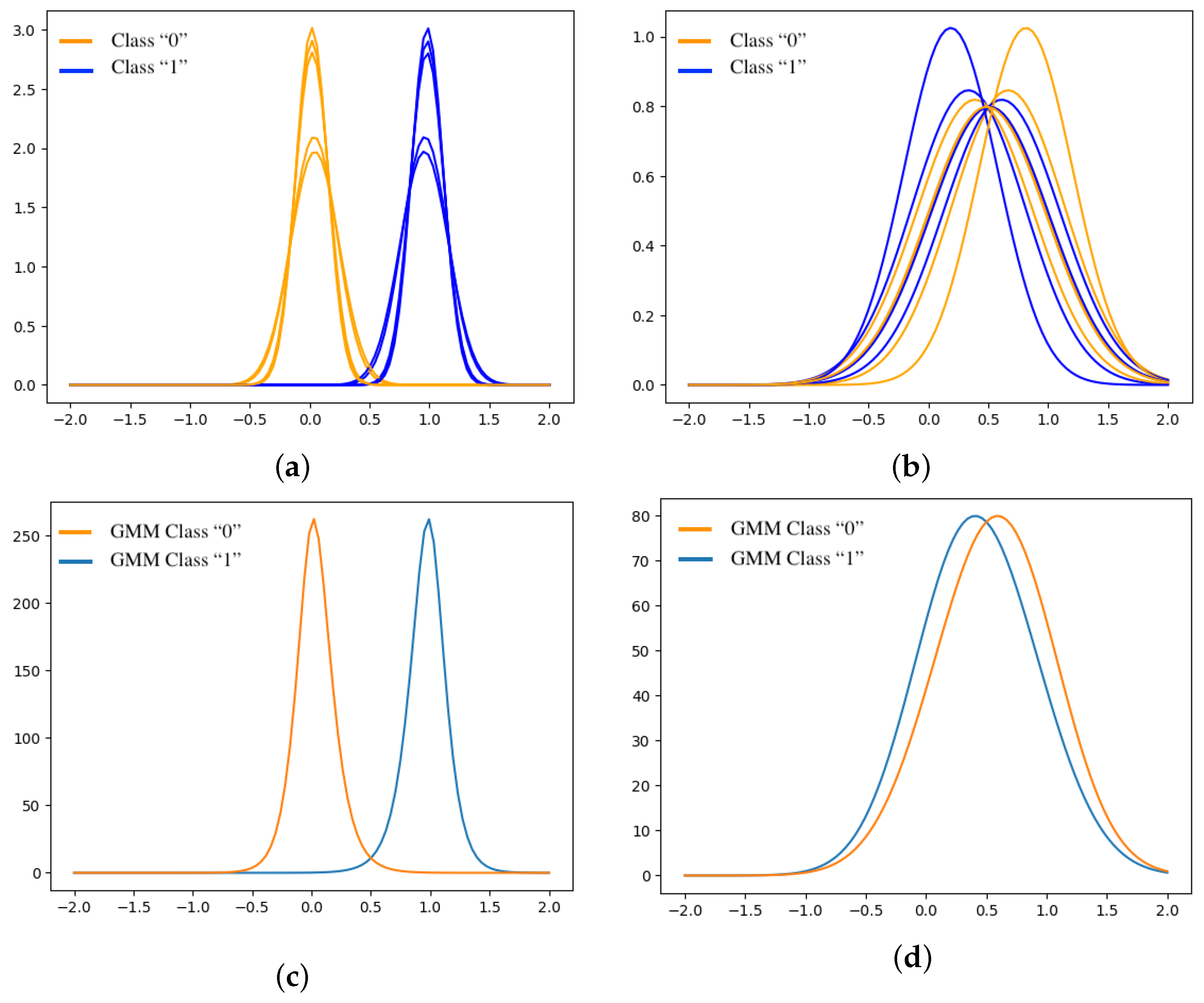
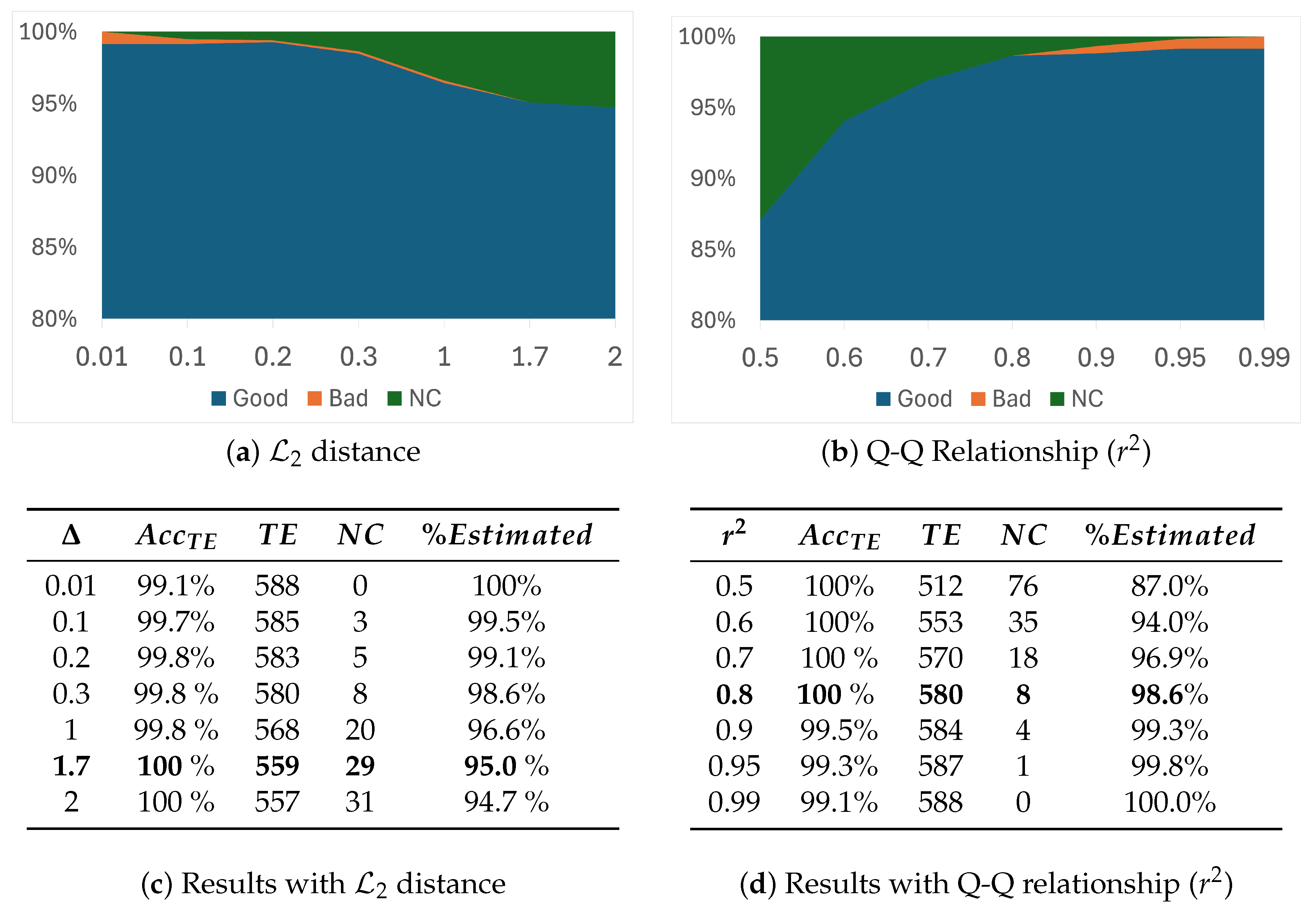
• A statistical module for estimating the final output of an ensemble set from the Bayesian architecture is proposed. Two metrics are explored: the ${\mathcal{L}}_2$ distance between Gaussian mixture models (divergence between probability functions) and the relationship between the estimated probability of the classes using a quantile comparison approach.
• The method is evaluated for a Blueberry data set where the images are classified according to the wax bloom content of the blueberries [56]. To further validate the proposed method, state-of-the-art methods for combining the outputs of the Bayesian ensemble and detecting potential misclassification are implemented and used for comparison.

Finally, the discussion and conclusions of this work are presented in Section 4 and Section 5, respectively.

2. Materials and Methods

A very small Bayesian–CNN model is proposed to classify images of blueberries according to their wax bloom content. In order to capture the uncertainty of the final estimation, a statistical approach is added to the model to perform the final output and determine whether a sample is well classified or not. The details of the Bayesian–CNN model implemented and the statistical module are described as follows. A scheme of the proposed method is displayed in Figure 1.

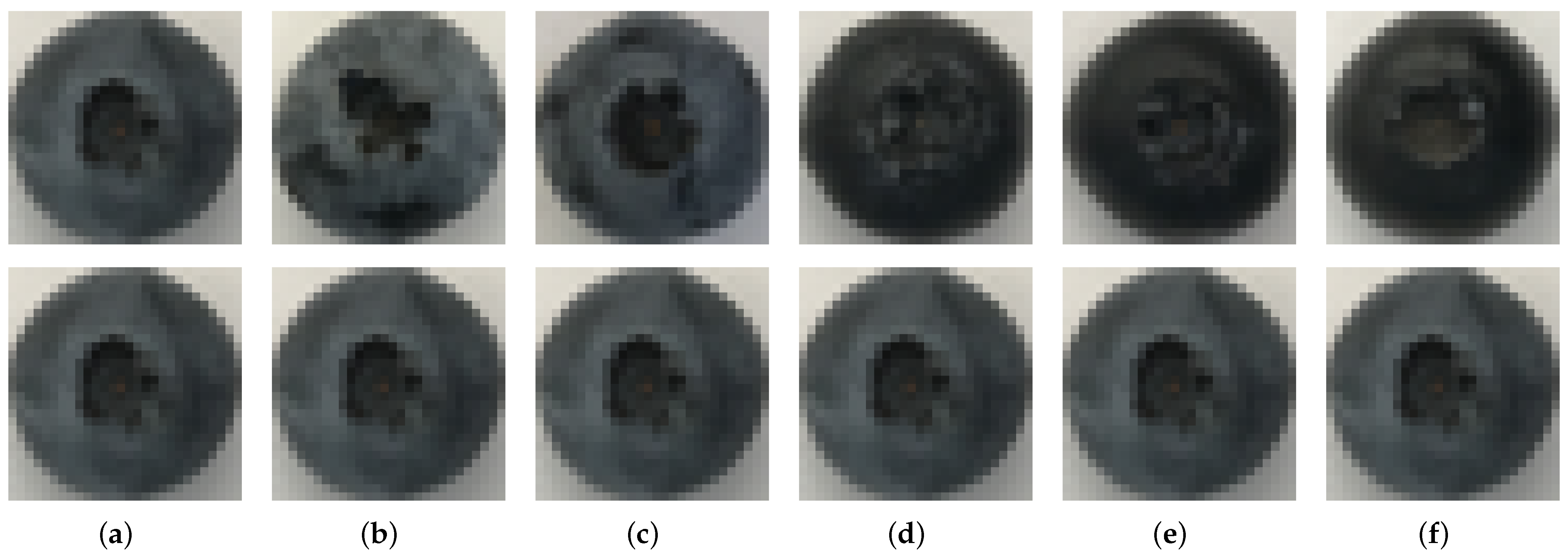
2.1. Blueberry Database

The blueberry database utilized in this study [56] was captured using an IPhone 7 with 0.5× zoom. Each blueberry was captured using a white background and placed 10 cm from the camera. Natural light was used with no flash (the images were captured between 9:00 a.m. and 13:00 p.m.). The image resolution was 3024 × 4032 pixels. Two sets of images were acquired. Firstly, 1484 blueberries with a visible wax bloom were captured and labeled as the “Bloom” set. For the second set, labeled as “NonBloom”, each blueberry was cleaned using a soft tissue in order to remove the wax bloom. Additional images of blueberries that did not originally have a wax bloom were also added to this set for a total of 1547 images. Two images were captured for each blueberry in both data sets: one on the scar side and the other on the flower side of the blueberry. All blueberries used in this data set were sourced from local supermarkets from three different brands: Hortifrut S.A, Jumbo, and Huertos Chile. An example of the images in the database is shown in Figure 2.

2.2. Shallow Bayesian–CNN Model

Given a set of inputs $\{x_1,x_2,x_3,\dots x_n\}$ with its respective outputs $\{y_1,y_2,y_3,\dots y_n\}$, it is desirable to model the function f such that $y=f\left(\mathbf{x}\right)$. With Bayesian inference, a prior distribution over the space of functions $p\left(f\right)$, is used. This distribution represents a prior belief as to which functions are likely to have generated the data. The likelihood is defined as $p\left(y\right|f,\mathbf{x})$ and, by using the Bayes rule, the posterior distribution may be found $p\left(f\right|\mathbf{x},y)$ given the input data set $\{\mathbf{x},y\}$. The output can be predicted for a new input $x^{*}$ by integrating over all possible functions f:

$$p\left(y^{*}\right|x^{*},\mathbf{x},y)=\int p\left(y^{*}\right|f^{*})p\left(f^{*}\right|x^{*},\mathbf{x},y)d{f}^{*}$$

(1)

Assuming that Equation (1) can be approximated by taking a finite set of random variables w and conditioning the model on it, the equation can be rewritten as follows:

$$p\left(y^{*}\right|x^{*},\mathbf{x},y)=\int p\left(y^{*}\right|f^{*})p\left(f^{*}\right|x^{*},w)p\left(w\right|\mathbf{x},y)d{f}^{*}dw$$

(2)

Since $p\left(w\right|\mathbf{x},y)$ is intractable, it can be approximated with a variational distribution $q\left(w\right)$, which has to be as close as possible to the posterior distribution obtained from the original model. In order to make those distributions as close as possible, the Kullback–Leibler (KL) divergence between the two distributions is minimized $KL\left(q\right(w\left)\right|\left|p\right(w|\mathbf{x},y))$. Since minimizing the Kullback–Leibler divergence is equivalent to maximizing the log evidence lower bound with respect to the variational parameters defining $q\left(w\right)$, the following expression can be maximized instead:

$$KLVI:=\int q(w)p(F|X,w)logp(Y|F)dFdw-KL(q(w)||p(w))$$

(3)

This expression is known as a variational inference, and is a standard technique in Bayesian modeling. Using this technique, a Bayesian convolutional network (BCNN) with two convolutional layers (8 and 4 filters, respectively) and a dense layer was implemented. The total number of parameters to be estimated during training was only 1052. The model was implemented in Keras using “conv_reparametrization” layers with swish activation. Normal distributions were assumed for the prior and posterior probability functions.

2.3. Binary Output Estimation and Potential Misclassification Detection

The Bayesian–CNN provides a model where weights are modeled as density functions, with the mean and standard deviation estimated during training. In order to use the model to perform a prediction, several weights sampled from each density function are drawn to achieve a set of different models and therefore a set of estimations (see Bayesian ensemble in Figure 1). The final output should be a combination of all predictions. For a set of n ensembles, the predicted probability for each label (class) c is as follows:

$$p_c={\displaystyle \frac{1}{n}}\sum _{i=1}^n{p}_c^i,$$

(4)

where class $c=0,1$. The predicted label can be computed as the class with higher probability:

$$label=argmax\{p_{c=0},p_{c=1}\}$$

(5)

When the classes are perfectly separable, the output for each Bayesian model in the ensemble is as in Figure 3a, where the output mean and standard deviation estimated are reported for an ensemble of 100 models (100 samples). As can be appreciated, the mean probability for class “0” is approximately one in each sample, with a very small standard deviation, while class “1”, on the other hand, has a mean probability of zero and also a very small standard deviation. In this case, is easy to discriminate between the classes, and the Bayesian model shows that it is very certain about the predicted output. Figure 3b, on the contrary, shows that both classes have a bigger standard deviation for all the predicted samples (the output of each Bayesian model) and it is not easy to differentiate which class has the highest probability. In this case, the input image may not be well classified since the uncertainty for each class is high.

Two metrics are proposed to determine if the Bayesian ensemble is able to discriminate between classes and therefore filter out any potential misclassifications. The first metric is based on the ${\mathcal{L}}_2$ distance between a Gaussian mixture model and the second one is based on the quantile relationship between density functions.

The goal is to determine whether the output of the Bayesian ensemble corresponds to two different classes or just one class. In the case that the output corresponds to only one class, the model is not able to discriminate between the two classes and therefore cannot be used for prediction. Identifying when the model is not able to make a good decision is essential for having a more reliable model. The two proposed metrics are described as follows.

2.3.1. Euclidean Distance (${\mathcal{L}}_2$ ) Between Gaussian Mixture Models

As shown in Figure 3, when estimating the output from the Bayesian model, an estimation for the mean probability and standard deviation for each class is obtained (and for each model). Figure 3a,b show examples of the probability distribution obtained for 5 samples obtained from the model (5 models drawn from the Bayesian–CNN). In orange, the probability functions for class “Zero” and blue for the class “one” are shown. In Figure 3a, the results show consistency in the estimated probability functions, and it is easy to discriminate between the classes (this result corresponds to the same images used for Figure 3a). Figure 3b, on the other hand, shows that the probability function of both classes is quite close and that it is not easy to discriminate between them.

In order to establish a metric that indicates if the classes are separable or not, the divergence between probability density functions was used, in particular, the ${\mathcal{L}}_2$ distance (Euclidean distance between density functions). First, two probability density functions (Gaussian mixture models (GMMs)) were modeled with all the outputs of the Bayesian model: one GMM for each class. Figure 4c,d show the resulting GMM for the 5 samples drawn from the model and displayed in Figure 4a and Figure 4b, respectively.

In order to automatically establish if the final prediction may be considered as a trusted prediction, the Euclidean distance between the resulting Gaussian mixtures for each class was computed. If the distance is bigger than a set value $\Delta$, the model is properly separating the classes and therefore the estimation for each class is trustworthy. Otherwise, it will be considered that the ensemble Bayesian model was not able to accurately determine the class of the image.

The two Gaussian model mixtures $g_{c=0}\left(\mathbf{x}\right)$ and $g_{c=1}\left(\mathbf{x}\right)$ can be modeled as follows:

$$g_{c=0}\left(\mathbf{x}\right)=\sum _{i=1}^n{w}_i\mathcal{N}(\mathbf{x},{\mu }_i^{c=0},{\Sigma }_i^{c=0})$$

(6)

and

$$g_{c=1}\left(x\right)=\sum _{i=1}^n{w}_i\mathcal{N}(\mathbf{x},{\mu }_i^{c=1},{\Sigma }_i^{c=1})$$

(7)

where n is the number of estimates made using the Bayesian model (set of Bayesian models), $w_i={\displaystyle \frac{1}{n}}$ is the weight of each Gaussian, $\mu$ is the mean of each Gaussian, and $\Sigma$ is the covariance. The ${\mathcal{L}}_2$ distance between two Gaussian distributions can then be computed using the following:

$${\mathcal{L}}_2(g_{c=0},g_{c=1})=\int \{g_{c=0}^2\left(\mathbf{x}\right)-2g_{c=0}\left(\mathbf{x}\right)g_{c=1}\left(\mathbf{x}\right)+g_{c=1}^2\left(\mathbf{x}\right)\}d\mathbf{x}$$

(8)

This expression can be explicitly computed since the multiplication of two Gaussian distributions has a closed-form solution [57,58] as follows:

$$\int \mathcal{N}(\mathbf{x},{\mu }_1,{\sigma }_1)\mathcal{N}(\mathbf{x},{\mu }_2,{\sigma }_2)=\mathcal{N}({\mu }_1-{\mu }_2,0,{\sigma }_1^2+{\sigma }_2^2)$$

(9)

The final algorithm for estimating the class of a new observation is then computed as follows. A set of n samples is obtained from the Bayesian network. A Gaussian mixture model is computed for each class and then their ${\mathcal{L}}_2$ distance is computed. If the result is smaller than a threshold (${\mathcal{L}}_2<\Delta$), the model is not able to perform a robust estimate for the class of the input image. Otherwise (${\mathcal{L}}_2>=\Delta$), the output of the model is considered as a robust solution for the input image. The modeling of Gaussian mixtures with the output of the Bayesian model allows a final estimate to be defined that considers not only the estimated mean for the probabilities for each class but the standard deviation as well.

2.3.2. Quantile-to-Quantile Relationship Between Classes

Another approach that allows the relationship between samples of the the same density function to be established is quantile-to-quantile analysis. This is usually used to determine if a sample belongs to a normal distribution or not. In order to define a metric to determine how different the distributions of the two classes are, a similar approach is used, but the analysis considers the output for each class as two separate sets (instead of comparing each set with a normal distribution, the prediction of one class is compared against the predictions of the other class). In this case, the quantile analysis was performed over the two classes simultaneously by plotting the quantiles of each class and fitting the best line (regression model). If the fitted line has an $r^2$ close to one, it indicates that the two classes may come from the same distribution and therefore the model cannot discriminate between the two classes. In this case, the output of the model is considered as non-trustworthy. On the other hand, if the $r^2$ is very distant from one, it can be considered that they belong to two different distributions and therefore the two classes can be distinguished from the data.

The $r^2$ threshold that defines the boundary between what we consider as the samples belonging to the same distribution and those that we do not is set and discussed during the experimental section.

2.4. Implementation Details: Software and Hardware

All the experiments were implemented in Python 3.8.10 using the 2.8.0 version of Tensorflow and Keras. An nvidia RTX 3090 GPU was used in a PC using the Linux operating system (Ubuntu 22.04.5 LTS). The Euclidean distance between density functions (${\mathcal{L}}_2$) was implemented in Python from scratch using the closed-form solution (see expression (8) and (9)). The quantile metric was implemented using the library stats from scipy.

3. Experiments and Results

For all experiments, the database published in [56] and described in Section 2.1 was used. Three experiments were performed: first, the Bayesian–CNN ensemble model was compared with state-of-the-art small architectures (fewer than 6,000,000 parameters). In experiment 2, two metrics for detecting potential misclassifications were evaluated and compared with similar techniques from the state of the art. Experiment 3 reports results from using cross validation and compares performance considering the trade-off between accuracy and the number of samples considered as not classified.

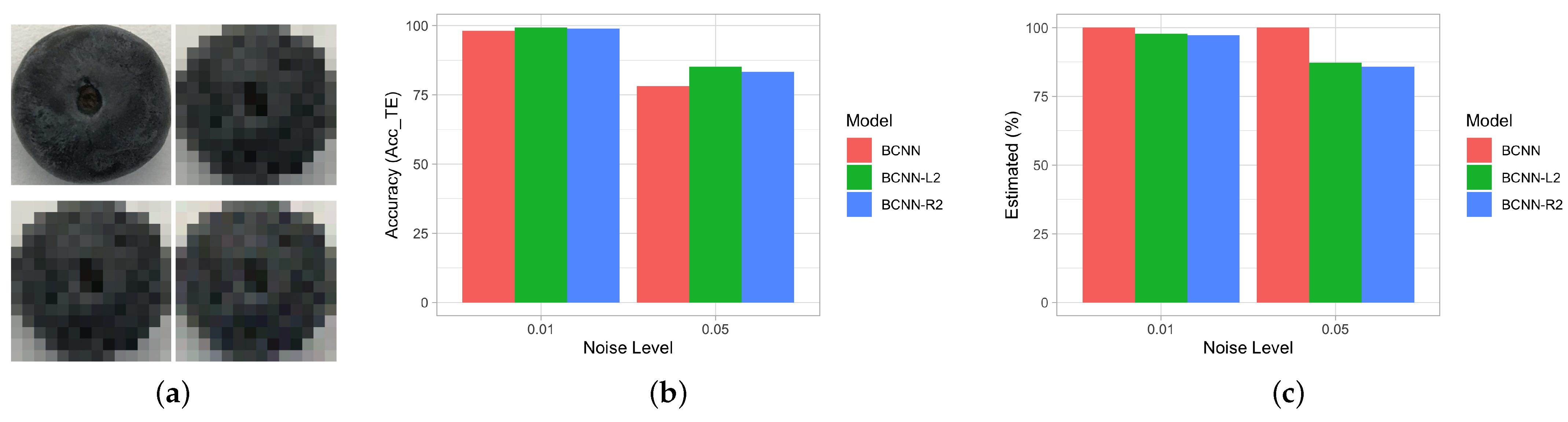
3.1. Bayesian–CNN Ensemble Model

The Bayesian–CNN model was trained using 1000 epochs and a learning rate of 0.001. Input images of 14 × 14 pixel resolution were used. A k-fold cross validation was performed (with k = 5) using all images in the database. The final accuracy obtained for the Bayesian–CNN model was $96.9\%$, with a standard deviation of $0.6$ and combining 100 samples (Bayesian models). An example of the training loss and accuracy curves obtained is shown in Figure 5a and Figure 5b, respectively. The resulting confusion matrix is displayed in Figure 5c.

Table 1. A comparison of accuracy results obtained used the proposed Bayesian–CNN model and several models from the literature.

Model	Parameters	Accuracy	Image Resolution
VGG16 [59]	134,268,738	99.2%	224 × 224
MobileNet [60]	5,148,154	98.4%	224 × 224
LeNet [61,62]	44,046	98.0%	28 × 28
Proposed BCNN	1052	96.9%	14 × 14
CNN	1426	92.0%	14 × 14

presents a comparison of several architectures reported in the literature. Only small architectures (fewer than 6,000,000 parameters ) were selected since the main goal of this work is to achieve a small model that could be used in small computer devices such as mobile phones. A VGG16 architecture trained using transfer learning was used as a reference model. This model achieved an accuracy of $99.1\%$ but with more than 134 million parameters. For comparison, several CNN architectures were also implemented. However, the smallest model that converges to a reasonable solution (1426 parameters) only achieves an accuracy of $92\%$. Smaller models did not converge and therefore were not able to predict reasonable results. These results show that the Bayesian approach not only helps in adding uncertainty to the model but also improves convergence when smaller architectures are used.

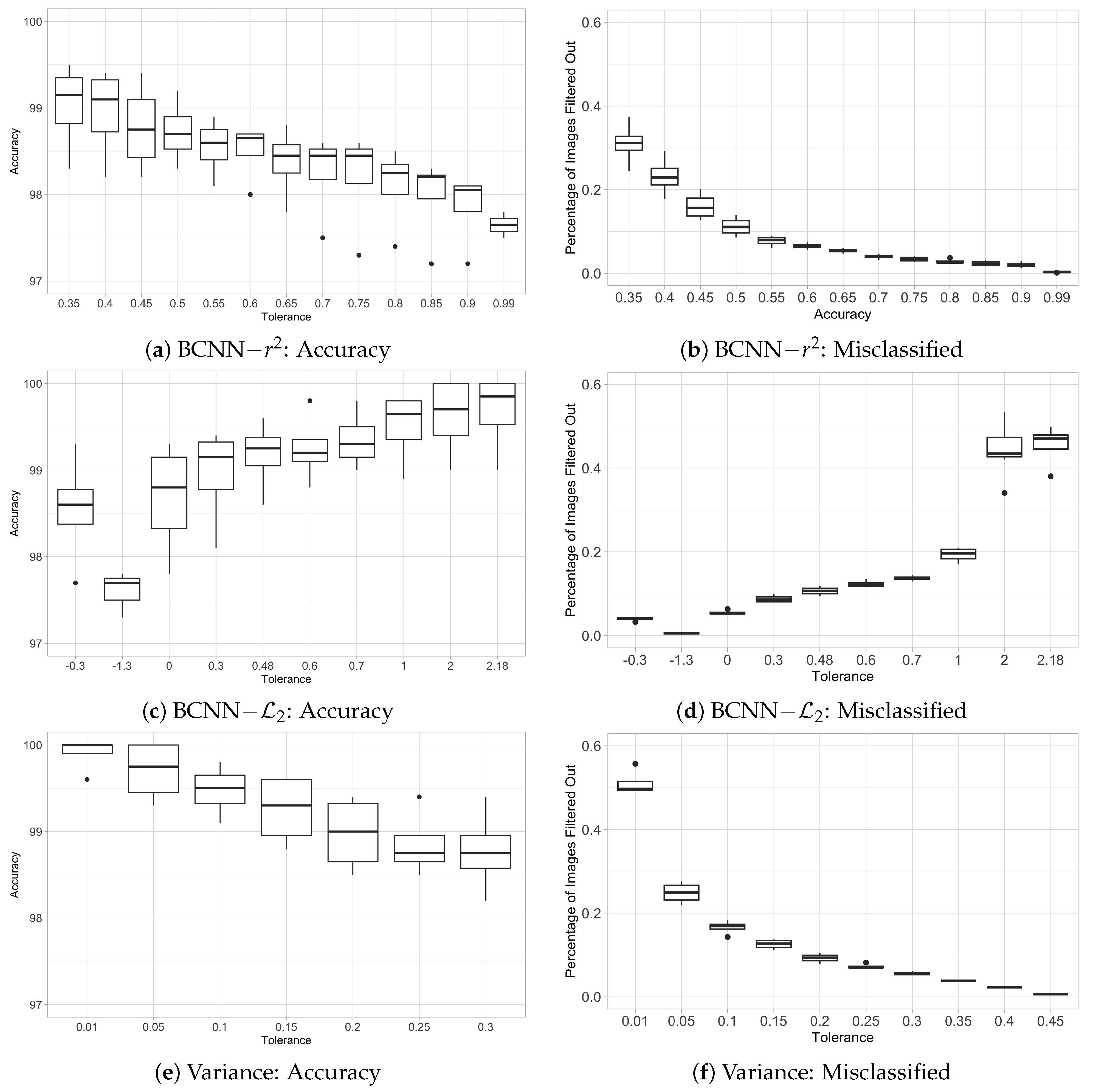
3.2. Potential Misclassification Detection Metrics

For this experiment, a random partition of the data was used to train the Bayesian–CNN model (train ($65\%$—1931 images), test ($19\%$—588 images), and validation ($17\%$—512 images)). The resulting prediction obtained for the test set was tested for potential misclassification using the two metrics proposed. For the case where the ${\mathcal{L}}_2$ distance between GMMs is used, several values for $\Delta$ were tested, where $\Delta$ is the minimum distance that the two GMMs modeled for each class should have in order to be considered as two separate distributions. If the ${\mathcal{L}}_2$ distance is less than $\Delta$, it was assumed that the Bayesian ensemble model was not able to achieve a trustworthy prediction, and therefore the results were considered as not classified. For each value of delta, the accuracy over the samples that are considered to have trustworthy prediction was computed as follows:

$$Ac{c}_{TE}={\displaystyle \frac{TP+TN}{TE}}$$

(10)

where $TE$ refers to the number of predictions by the model that are considered to be well classified (where ${\mathcal{L}}_2$ > $\Delta$), TP refers to the true positives, and TN refers to the true negatives. Additionally, the proportion of images that were classified was computed (after filtering out the images that are considered as not classified according to the ${\mathcal{L}}_2$ distance). The metric can be computed as follows:

$$Estimated={\displaystyle \frac{TE}{Total}}$$

(11)

where $Total$ corresponds to the total number of images in the test set.

Figure 6a,c show the results obtained for a set of different tolerances for the ${\mathcal{L}}_2$ distance (from 0.01 to 2). Figure 6a shows the percentage of images that are well classified for the Bayesian ensemble, those that are misclassified, and the images that are filtered out using the ${\mathcal{L}}_2$ distance (not classified). A desirable model is one that achieve a high accuracy (ideally $100\%$) with a minimum number of images filtered out. In this case, the tolerance value ($\Delta$) that achieves better results is 1.7 with an accuracy of $100\%$, but there are 29 images that are not classified.

A similar experiment using the second metric proposed (quantile–quantile relationship) was performed. The results are shown in Figure 6b,d. In this case, the best result is achieved when the tolerance value for the coefficient of determination $r^2$ is $0.8$. Using this value, an accuracy of $100\%$ is obtained, with only eight images not classified. Examples of images potentially misclassified by both proposed metrics are displayed in Figure 7. It may be noted that the latter metric ($r^2$) is able to achieve $100\%$ accuracy while eliminating fewer images than the first method (${\mathcal{L}}_2$). Therefore, $98.6\%$ of the data are classified with high certainty compared to only $95.0\%$ in the case when the ${\mathcal{L}}_2$ distance is used.

Additional experiments were performed that added noise to the images in the data set. Random noise with maximum values of 0.01 and and 0.05 were added to the image before testing them. The accuracy achieved by the BCNN model before and after filtering out the potentially misclassified images using the two method proposed is displayed in Figure 8. Adding noise deteriorates the accuracy obtained. However, the ${\mathcal{L}}_2$ shows better performance in both experiments. The number of images filtered out is lower in the case where this metric is used. It may be noted that, for this experiment, tolerance levels for ${\mathcal{L}}_2$ and $r^2$ were 0.2 and 0.8, respectively. It may also be noted that increasing the tolerance $\Delta$ for the ${\mathcal{L}}_2$ distance metric will provide better accuracy. However, it will drastically increase the number of images filtered out. Similarly, a decrease in tolerance for $r^2$ will improve accuracy at the expense of an increase in the number of images filtered out or not classified. Depending on the application, a trade-off between accuracy and the rate of estimated images can be established by varying the tolerance ($\Delta$ and $r^2$, respectively).

Two methods from the state of the art were implemented for comparison. The entropy-based method proposed by Al-Majed et al. [53] was used to compare with the results of the Bayesian ensemble (BCNN). The variance threshold reported by Joshi et al. [55] was used for detecting potential misclassification and to compare with the two metrics proposed in this work.

Table 2. The results obtained for the experiments performed for the proposed method and state-of-the-art techniques. Experiments were performed for the original data set and two levels of added noise. For each method, the accuracy ($Ac{c}_{TE}$), number of non-classified images ($NC$), and percentage of estimated images are reported (Estimated).

Noise Level	Model	${\mathit{Acc}}_{\mathit{TE}}$	$\mathit{NC}$	%$\mathit{Estimated}$
Original data set	BCNN-mean	$99.1\%$	-	$100\%$
	BCNN-Entropy [53]	97.8%	-	$100\%$
	BCNN-${\mathcal{L}}_2$	$100\%$	29	$95\%$
	BCNN-$r^2$	$100\%$	8	$98.6\%$
	BCNN-Variance [55]	$100\%$	43	$92.6\%$
Added noise (0.01)	BCNN-mean	$98.1\%$	-	$100\%$
	BCNN-Entropy [53]	$97.6\%$	-	$100\%$
	BCNN-${\mathcal{L}}_2$	$99.3\%$	13	$97.78\%$
	BCNN-$r^2$	$99\%$	16	$97.27\%$
	BCNN-Variance [55]	$100\%$	51	$91.15\%$
Added noise (0.05)	BCNN-mean	$78.1\%$	-	$100\%$
	BCNN-Entropy [53]	$79.3\%$	-	$100\%$
	BCNN-${\mathcal{L}}_2$	$85.2\%$	75	$87.84\%$
	BCNN-$r^2$	$83.3\%$	84	$85.71\%$
	BCNN-Variance [55]	$88.7\%$	199	$66.16\%$

shows the accuracy obtained for all methods after filtering the images with high uncertainty, for the original set, and for two additional data sets where two different levels of noise were added to the original set. Additionally, the number of images filtered out ($NC$ not classified) and the final proportion of images estimated ($\%Estimated$) are also reported. As can be appreciated, using just the mean as a metric for combining the models achieved better results for the original set and for the set with a low level of noise. On the contrary, when levels of noise are higher, the entropy metric shows a slightly better performance (78.1% versus 79.3%).

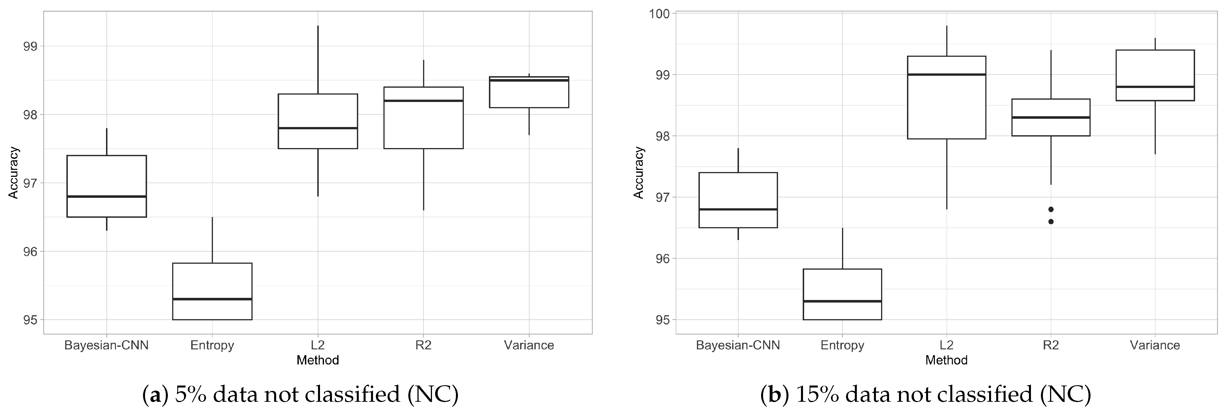
3.3. Trade-Off Between Accuracy and Number of Non-Classified Images (Filtered Out)

It may be noted that it is not straightforward to compare the metrics in terms of accuracy. All the metrics proposed have to deal with the trade-off between increasing accuracy and decreasing the number of images filtered out. The key value that regulates this performance is the tolerance chosen for each metric.

To compute the overall performance of the proposed metrics, the prediction results for the k-fold cross-validation method implemented in experiment 1 were used (all images in the database were used for the k-fold cross validation). Similar to the previous experiment, 100 Bayesian models were ensembled using the two proposed metrics (Euclidean distance ${\mathcal{L}}_2$ and $r^2$) and the variance method. The results regarding the accuracy of each method as a function of the tolerance used to detect potential misclassification samples in order to filter them out are shown in Figure 9a,c,e for the metrics ${\mathcal{L}}_2$, $r^2$, and variance. The distribution of the number of non-classified images (NC) is shown in Figure 9b,d,e for each method, respectively.

The tolerance range chosen for the $r^2$ metric (see Figure 9a) was between $0.35$ and $0.99$. $r^2$ is the linear relationship between the samples of the two classes; therefore, the tolerance should be chosen to discriminate such linearity. A smaller value increases accuracy but at the expense of eliminating a larger proportion of images as shown in Figure 9b. Values between 0.7 and 0.9 are preferable since they represent a linear relation of 70 and 90 percent, respectively. These values achieve an accuracy rate above $98\%$.

Figure 9c shows the case of using the Euclidean distance ${\mathcal{L}}_2$ between GMMs as a metric. In this case, the tolerance range is chosen as between 0.001 and 250. A logarithmic scale ($lo{g}_{10}$) was used to plot the results as, the larger the accepted distance (tolerance), the better the accuracy of the model. However, this has an impact on the number of images filtered out (see Figure 9d).

Finally, in Figure 9e, the results obtained for the variance discrimination method for filtering out potential misclassifications are presented. The values range between 0.01 and 0.3. Values larger than 0.3 result in rapidly decreasing accuracy. Note that both metrics, ${\mathcal{L}}_2$ and variance, achieve an accuracy of $100\%$; however, in both cases, this occurs at the expense of eliminating a great proportion of the data (see Figure 9d,f).

Figure 10 shows the distribution of accuracy obtained for all models (for all defined tolerances). In order to set a fair comparison, the number of deleted images (detected as not classified) was set to $5\%$ (see Figure 10a) and $15\%$ (see Figure 10b). The results demonstrate that all methods performed similarly; however, the variance method exhibited better accuracy while deleting more images ($15\%$ in this case). For comparison, Figure 10a,b also show the results for the baseline BCNN model (without the module for discriminating potential misclassifications reported in experiment 1) and the same model when the entropy method for detecting the final solution (instead of the mean) was used.

As has been established, the accuracy and the number of “Not Classified” images directly depends on the chosen value for the tolerance metric. The results presented in Figure 9 can be used to set the tolerance value required for each metric according to the expected accuracy or expected number of images that the user is willing to accept as not classified. For instance, when the target is to achieve an algorithm within a range of non-classified images around $5\%$, the tolerance value to use for the ${\mathcal{L}}_2$, $r^2$, and variance metrics should be approximately 0.65, 1, and 0.35, respectively.

Table 3. A comparison of accuracy results obtained used the proposed Bayesian–CNN model and several models from the literature.

Model	${\mathit{Acc}}_{\mathit{TE}}$	$\mathit{NC}$ (%)	%$\mathit{Estimated}$
BCNN-mean	96.98 ± 0.66%	-	100%
BCC-Entropy [53]	95.52 ± 0.7%	-	100%
BCNN-${\mathcal{L}}_2$	98.72 ± 0.54%	6.89 ± 1.65%	$93.10\pm 0.01\%$
BCNN-$r^2$	$98.38\pm 0.34\%$	$6.36\pm 2.28\%$	$93.63\pm 0.02\%$
BCNN-Variance [55]	$98.80\pm 0.46\%$	6.26 ± 1.60%	$93.73\pm 0.01\%$
BCNN-${\mathcal{L}}_2$ + $r^2$ + Variance	$98.64\pm 0.56\%$	$5.54\pm 1.60\%$	$94.46\pm 1.60\%$

shows the results obtained for the tolerance values for the three metrics when using the prediction results of the five models (with a 100-Bayesian ensemble).

As expected, the results are similar to the distribution shown in Figure 10. The baseline models (BCNN-mean and BCNN-Entropy) are also reported for comparison. As may be noticed, all reported metrics improve the accuracy between $1.4\%$ and $1.7\%$ when eliminating around $6\%$ of the data. The table also reports the result of combining the three metrics by selecting the images that were detected by at least two of the methods as not classified. In this case, the overall result is maintained while eliminating slightly fewer images (around $5\%$).

4. Discussion

The use of two alternative metrics to filter out potentially misclassified images from a Bayesian–CNN model and to improve the accuracy of the remaining data has been proposed. One metric was based on the coefficient of determination $r^2$ from the quantile–quantile relationship between samples and the other one was based on the Euclidean ${\mathcal{L}}_2$ distance between probability density functions. Both showed a competitive performance compared to the state of the art and were able to improve the accuracy of a Bayesian–CNN ensemble model from $96.98\%$ to $98.72\pm 0.54\%$ and $98.38\pm 0.34\%$ for the ${\mathcal{L}}_2$ and $r^2$ metrics, respectively. This improvement made the results of the Bayesian–CNN ensemble model comparable to the results obtained with bigger models like MobileNet, which requires more than 5 million parameters and higher image resolution to achieve similar results. However, this improvement was achieved at the expense of computing several predictions for each image (Bayesian ensemble) and adding an extra module for detecting and filtering out potential misclassifications. Therefore, this method is suitable for developing a computational application where the lack of memory is compensated for with processing power. Note that the increase in computation is mainly due to the Bayesian approach. The computation time required for the final module that filtered out potentially misclassified images is insignificant in comparison to the time required for making n predictions of the ensemble.

This method was applied in order to detect wax bloom in blueberry images acquired using a mobile phone in a controlled environment. The reliability of these results was demonstrated using a 5-fold cross-validation method. The proposed metric used to filter out potentially misclassified data could be applied to any types of data. This module is only a post-processing analysis that may be used after any ensemble of models (not necessarily Bayesian).

The main advantage of using the ${\mathcal{L}}_2$ distance is that it is known for being a robust metric for computing divergence (distance) between probability density functions. It uses not only the output mean of each prediction in the Bayesian model but also its variance. This would be less prone to outliers than the variance method, and the final GMM modeled for each class may not need a large number of samples to represent the density functions well. $r^2$, on the other hand, may improve its robustness by increasing the number of samples used to fit the line that defines the relationship between the quantile data of the classes. However, an increase in the number of ensembles directly affects the computing cost of the final model.

The ${\mathcal{L}}_2$ has a computational complexity that depends on the number of Gaussians used in the mixture model. The larger the number of samples n drawn from the Bayesian model, the more computationally expensive the algorithm becomes ($n^2$). The quantile analysis also depends on the number of samples used to fit the line. However, in this case, the optimization method used for fitting the line is simple and takes less time than computing the ${\mathcal{L}}_2$ distance between density functions.

The key process for maximizing the performance of the proposed methods is to choose an appropriate tolerance value. This value not only determines the accuracy obtained by the model but the number of images sorted as not classified as well. A set of experiments with a range of tolerance values will give an idea of the best possible values by analyzing the trade-off between the accuracy obtained and number of images eliminated (not classified). This process is not computationally expensive since it is computed after all predictions are made.

5. Conclusions

It has been shown that a small Bayesian–CNN can be implemented for classifying blueberry images according to their wax bloom content. Only a few parameters were enough to achieve $96.98\pm 0.66\%$ accuracy. In order to improve this performance, two metrics were proposed to filter out potential misclassifications. The first metric is based on the ${\mathcal{L}}_2$ distance between Gaussian mixture models while the second metric is based on a quantile analysis of the binary class predictions ($r^2$). Both metrics are able to filter out potential misclassifications and improve result accuracy up to $98.72\pm 0.54\%$ and $98.38\pm 0.34\%$ for ${\mathcal{L}}_2$ and $r^2$, respectively, while approximately $6\%$ of the data are filtered out (not classified).

As a potential continuation for this research with respect to the task of berry wax bloom classification, this method may be used to evaluate the impact on the mechanical sorting of blueberries and the implementation of this method in the wild using a small computer device (for example, a cellphone). In terms of future work related to the proposed metrics, two lines of research will be explored. Firstly is the use of the GMM and ${\mathcal{L}}_2$ not just for potential misclassification detection but also as a method for combining, under a robust metric, the predictions of the ensemble. A second challenge is to reduce the number of non-classified images. This can be performed by combining several metrics, like those proposed in this work.

References

1. Kalt, W.; Cassidy, A.; Howard, L.R.; Krikorian, R.; Stull, A.J.; Tremblay, F.; Zamora-Ros, R. Recent Research on the Health Benefits of Blueberries and Their Anthocyanins. Adv. Nutr. 2020, 11, 224–236. [Google Scholar] [CrossRef]
2. Huamán, R.; Soto, F.; Ríos, A.; Paredes, E. International market concentration of fresh blueberries in the period 2001–2020. Humanit. Soc. Sci. Commun. 2023, 10, 967. [Google Scholar] [CrossRef]
3. Mainland, C.M.; Frederick, V. Coville and the History of North American Highbush Blueberry Culture. Int. J. Fruit Sci. 2012, 12, 4–13. [Google Scholar] [CrossRef]
4. Lobos, G.A.; Bravo, C.; Valdés, M.; Graell, J.; Lara Ayala, I.; Beaudry, R.M.; Moggia, C. Within-plant variability in blueberry (Vaccinium corymbosum L.): Matur. Harvest Position Canopy Influ. Fruit Firmness Harvest Postharvest. Postharvest Biol. Technol. 2018, 146, 26–35. [Google Scholar] [CrossRef]
5. Ktenioudaki, A.; O’Donnell, C.P.; Emond, J.P.; do Nascimento Nunes, M.C. Blueberry supply chain: Critical steps impacting fruit quality and application of a boosted regression tree model to predict weight loss. Postharvest Biol. Technol. 2021, 179, 111590. [Google Scholar] [CrossRef]
6. Funes, C.F.; Escobar, L.; Kirschbaum, D. Occurrence and population fluctuations of Drosophila suzukii (Diptera: Drosophilidae) in blueberry crops of subtropical Argentina. Acta Hortic. 2023, 1357, 257–264. [Google Scholar] [CrossRef]
7. Yan, Y.; Castellarin, S.D. Blueberry water loss is related to both cuticular wax composition and stem scar size. Postharvest Biol. Technol. 2022, 188, 111907. [Google Scholar] [CrossRef]
8. Chu, W.; Gao, H.; Chen, H.; Fang, X.; Zheng, Y. Effects of cuticular wax on the postharvest quality of blueberry fruit. Food Chem. 2018, 239, 68–74. [Google Scholar] [CrossRef]
9. Loypimai, P.; Paewboonsom, S.; Damerow, L.; Blanke, M.M. The wax bloom on blueberry: Application of luster sensor technology to assess glossiness and the effect of polishing as a fruit quality parameter. J. Appl. Bot. Food Qual. 2017, 90, 158. [Google Scholar] [CrossRef]
10. Gill, H.S.; Murugesan, G.; Mehbodniya, A.; Sekhar Sajja, G.; Gupta, G.; Bhatt, A. Fruit type classification using deep learning and feature fusion. Comput. Electron. Agric. 2023, 211, 107990. [Google Scholar] [CrossRef]
11. Sa, I.; Ge, Z.; Dayoub, F.; Upcroft, B.; Perez, T.; McCool, C. DeepFruits: A Fruit Detection System Using Deep Neural Networks. Sensors 2016, 16, 1222. [Google Scholar] [CrossRef] [PubMed]
12. Bargoti, S.; Underwood, J. Deep fruit detection in orchards. In Proceedings of the 2017 IEEE International Conference on Robotics and Automation (ICRA), Singapore, 29 May–3 June 2017; pp. 3626–3633. [Google Scholar] [CrossRef]
13. Castro, W.; Oblitas, J.; De-La-Torre, M.; Cotrina, C.; Bazán, K.; Avila-George, H. Classification of Cape Gooseberry Fruit According to its Level of Ripeness Using Machine Learning Techniques and Different Color Spaces. IEEE Access 2019, 7, 27389–27400. [Google Scholar] [CrossRef]
14. Pacheco, W.; López, F. Tomato classification according to organoleptic maturity (coloration) using machine learning algorithms K-NN, MLP, and K-Means Clustering. In Proceedings of the 2019 XXII Symposium on Image, Signal Processing and Artificial Vision (STSIVA), Bucaramanga, Colombia, 24–26 April 2019; pp. 1–5. [Google Scholar] [CrossRef]
15. Liu, X.; Chen, S.; Aditya, S.; Sivakumar, N.; Dcunha, S.; Qu, C.; Taylor, C.J.; Das, J.; Kumar, V. Robust Fruit Counting: Combining Deep Learning, Tracking, and Structure from Motion. In Proceedings of the 2018 IEEE/RSJ International Conference on Intelligent Robots and Systems (IROS), Madrid, Spain, 1–5 October 2018; pp. 1045–1052. [Google Scholar] [CrossRef]
16. Yu, Y.; Zhang, K.; Yang, L.; Zhang, D. Fruit detection for strawberry harvesting robot in non-structural environment based on Mask-RCNN. Comput. Electron. Agric. 2019, 163, 104846. [Google Scholar]
17. Gupta, S.; Tripathi, A.K. Fruit and vegetable disease detection and classification: Recent trends, challenges, and future opportunities. Eng. Appl. Artif. Intell. 2024, 133, 108260. [Google Scholar] [CrossRef]
18. Li, Z.; Xu, R.; Li, C.; Munoz, P.; Takeda, F.; Leme, B. In-field blueberry fruit phenotyping with a MARS-PhenoBot and customized BerryNet. Comput. Electron. Agric. 2025, 232, 110057. [Google Scholar] [CrossRef]
19. Gai, R.; Gao, J.; Xu, G. HPPEM: A High-Precision Blueberry Cluster Phenotype Extraction Model Based on Hybrid Task Cascade. Agronomy 2024, 14, 1178. [Google Scholar] [CrossRef]
20. Altalak, M.; uddin, M.A.; Alajmi, A.; Rizg, A. Smart Agriculture Applications Using Deep Learning Technologies: A Survey. Appl. Sci. 2022, 12, 5919. [Google Scholar] [CrossRef]
21. Seng, K.P.; Ang, L.; Schmidtke, L.M.; Rogiers, S.Y. Computer Vision and Machine Learning for Viticulture Technology. IEEE Access 2018, 6, 67494–67510. [Google Scholar] [CrossRef]
22. Li, H.; Lee, W.S.; Wang, K. Identifying blueberry fruit of different growth stages using natural outdoor color images. Comput. Electron. Agric. 2014, 106, 91–101. [Google Scholar] [CrossRef]
23. Yang, C.; Lee, W.S.; Gader, P. Hyperspectral band selection for detecting different blueberry fruit maturity stages. Comput. Electron. Agric. 2014, 109, 23–31. [Google Scholar] [CrossRef]
24. Ahmad, A.; Saraswat, D.; El Gamal, A. A survey on using deep learning techniques for plant disease diagnosis and recommendations for development of appropriate tools. Smart Agric. Technol. 2023, 3, 100083. [Google Scholar] [CrossRef]
25. Barbole, D.K.; Jadhav, P.M.; Patil, S.B. A Review on Fruit Detection and Segmentation Techniques in Agricultural Field. In Proceedings of the Second International Conference on Image Processing and Capsule Networks, Bangkok, Thailand, 27–28 May 2021; pp. 269–288. [Google Scholar] [CrossRef]
26. Yang, B.; Xu, Y. Applications of deep-learning approaches in horticultural research: A review. Hortic. Res. 2021, 8, 123. [Google Scholar] [CrossRef]
27. Zhu, L.; Spachos, P.; Pensini, E.; Plataniotis, K.N. Deep learning and machine vision for food processing: A survey. Curr. Res. Food Sci. 2021, 4, 233–249. [Google Scholar] [CrossRef] [PubMed]
28. Zhao, C.; Zhang, Y.; Du, J.; Guo, X.; Wen, W.; Gu, S.; Wang, J.; Fan, J. Crop Phenomics: Current Status and Perspectives. Front. Plant Sci. 2019, 10, 714. [Google Scholar] [CrossRef]
29. Yang, W.; Feng, H.; Zhang, X.; Zhang, J.; Doonan, J.H.; Batchelor, W.D.; Xiong, L.; Yan, J. Crop Phenomics and High-Throughput Phenotyping: Past Decades, Current Challenges, and Future Perspectives. Mol. Plant 2020, 13, 187–214. [Google Scholar] [CrossRef]
30. Rossi, R.; Leolini, C.; Costafreda-Aumedes, S.; Leolini, L.; Bindi, M.; Zaldei, A.; Moriondo, M. Performances Evaluation of a Low-Cost Platform for High-Resolution Plant Phenotyping. Sensors 2020, 20, 3150. [Google Scholar] [CrossRef]
31. Tausen, M.; Clausen, M.; Moeskjær, S.; Shihavuddin, A.; Dahl, A.B.; Janss, L.; Andersen, S.U. Greenotyper: Image-Based Plant Phenotyping Using Distributed Computing and Deep Learning. Front. Plant Sci. 2020, 11, 1181. [Google Scholar] [CrossRef]
32. Quiroz, I.A.; Alférez, G.H. Image recognition of Legacy blueberries in a Chilean smart farm through deep learning. Comput. Electron. Agric. 2020, 168, 105044. [Google Scholar] [CrossRef]
33. Feng, W.; Liu, M.; Sun, Y.; Wang, S.; Wang, J. The Use of a Blueberry Ripeness Detection Model in Dense Occlusion Scenarios Based on the Improved YOLOv9. Agronomy 2024, 14, 1860. [Google Scholar] [CrossRef]
34. Ni, X.; Takeda, F.; Jiang, H.; Yang, W.Q.; Saito, S.; Li, C. A deep learning-based web application for segmentation and quantification of blueberry internal bruising. Comput. Electron. Agric. 2022, 201, 107200. [Google Scholar] [CrossRef]
35. Zhang, M.; Jiang, Y.; Li, C.; Yang, F. Fully convolutional networks for blueberry bruising and calyx segmentation using hyperspectral transmittance imaging. Biosyst. Eng. 2020, 192, 159–175. [Google Scholar] [CrossRef]
36. Ni, X.; Li, C.; Jiang, H.; Takeda, F. Deep learning image segmentation and extraction of blueberry fruit traits associated with harvestability and yield. Hortic. Res. 2020, 7, 110. [Google Scholar] [CrossRef]
37. Gonzalez, S.; Arellano, C.; Tapia, J.E. Deepblueberry: Quantification of Blueberries in the Wild Using Instance Segmentation. IEEE Access 2019, 7, 105776–105788. [Google Scholar] [CrossRef]
38. Ni, X.; Li, C.; Jiang, H.; Takeda, F. Three-dimensional photogrammetry with deep learning instance segmentation to extract berry fruit harvestability traits. ISPRS J. Photogramm. Remote Sens. 2021, 171, 297–309. [Google Scholar] [CrossRef]
39. Tan, K.; Lee, W.S.; Gan, H.; Wang, S. Recognising blueberry fruit of different maturity using histogram oriented gradients and colour features in outdoor scenes. Biosyst. Eng. 2018, 176, 59–72. [Google Scholar] [CrossRef]
40. MacEachern, C.B.; Esau, T.J.; Schumann, A.W.; Hennessy, P.J.; Zaman, Q.U. Detection of fruit maturity stage and yield estimation in wild blueberry using deep learning convolutional neural networks. Smart Agric. Technol. 2023, 3, 100099. [Google Scholar] [CrossRef]
41. Ropelewska, E.; Koniarski, M. A novel approach to authentication of highbush and lowbush blueberry cultivars using image analysis, traditional machine learning and deep learning algorithms. Eur. Food Res. Technol. 2024, 251, 193–204. [Google Scholar] [CrossRef]
42. Niedbała, G.; Kurek, J.; Świderski, B.; Wojciechowski, T.; Antoniuk, I.; Bobran, K. Prediction of Blueberry (Vaccinium corymbosum L.) Yield Based on Artificial Intelligence Methods. Agriculture 2022, 12, 2089. [Google Scholar] [CrossRef]
43. Chan, C.; Nelson, P.R.; Hayes, D.J.; Zhang, Y.J.; Hall, B. Predicting Water Stress in Wild Blueberry Fields Using Airborne Visible and Near Infrared Imaging Spectroscopy. Remote Sens. 2021, 13, 1425. [Google Scholar] [CrossRef]
44. Hennessy, P.J.; Esau, T.J.; Schumann, A.W.; uz Zaman, Q.; Corscadden, K.W.; Farooque, A.A. Evaluation of Cameras and Image Distance for CNN-Based Weed Detection in Wild Blueberry. Smart Agric. Technol. 2021, 2, 100030. [Google Scholar] [CrossRef]
45. Wang, Z.; Hu, M.; Zhai, G. Application of Deep Learning Architectures for Accurate and Rapid Detection of Internal Mechanical Damage of Blueberry Using Hyperspectral Transmittance Data. Sensors 2018, 18, 1126. [Google Scholar] [CrossRef] [PubMed]
46. Barbosa Júnior, M.R.; dos Santos, R.G.; de Azevedo Sales, L.; Vargas, R.B.S.; Deltsidis, A.; de Oliveira, L.P. Image-based and ML-driven analysis for assessing blueberry fruit quality. Heliyon 2025, 11, e42288. [Google Scholar] [CrossRef]
47. Fan, S.; Li, C.; Huang, W.; Chen, L. Data Fusion of Two Hyperspectral Imaging Systems with Complementary Spectral Sensing Ranges for Blueberry Bruising Detection. Sensors 2018, 18, 4463. [Google Scholar] [CrossRef]
48. Moggia, C.; Graell, J.; Lara, I.; Schmeda-Hirschmann, G.; Thomas-Valdés, S.; Lobos, G.A. Fruit characteristics and cuticle triterpenes as related to postharvest quality of highbush blueberries. Sci. Hortic. 2016, 211, 449–457. [Google Scholar] [CrossRef]
49. Abdar, M.; Pourpanah, F.; Hussain, S.; Rezazadegan, D.; Liu, L.; Ghavamzadeh, M.; Fieguth, P.; Cao, X.; Khosravi, A.; Acharya, U.R.; et al. A review of uncertainty quantification in deep learning: Techniques, applications and challenges. Inf. Fusion 2021, 76, 243–297. [Google Scholar] [CrossRef]
50. Milosevic, M.; Ciric, V.; Milentijevic, I. Network Intrusion Detection Using Weighted Voting Ensemble Deep Learning Model. In Proceedings of the 2024 11th International Conference on Electrical, Electronic and Computing Engineering (IcETRAN), Nis, Serbia, 3–6 June 2020; pp. 1–6. [Google Scholar] [CrossRef]
51. Zhang, J.; Li, F.; Ye, F. An Ensemble-based Network Intrusion Detection Scheme with Bayesian Deep Learning. In Proceedings of the ICC 2020 IEEE International Conference on Communications (ICC), Dublin, Ireland, 7–11 June 2020; pp. 1–6. [Google Scholar] [CrossRef]
52. Abdullah, A.A.; Hassan, M.M.; Mustafa, Y.T. Leveraging Bayesian deep learning and ensemble methods for uncertainty quantification in image classification: A ranking-based approach. Heliyon 2024, 10, e24188. [Google Scholar] [CrossRef] [PubMed]
53. Al-Majed, R.; Hussain, M. Entropy-Based Ensemble of Convolutional Neural Networks for Clothes Texture Pattern Recognition. Appl. Sci. 2024, 14, 10730. [Google Scholar] [CrossRef]
54. Njieutcheu Tassi, C.R. Bayesian Convolutional Neural Network: Robustly Quantify Uncertainty for Misclassifications Detection. In Proceedings of the Pattern Recognition and Artificial Intelligence, Istanbul, Turkey, 22–23 December 2019; Djeddi, C., Jamil, A., Siddiqi, I., Eds.; Springer International Publishing: Cham, Switzerland, 2020; pp. 118–132. [Google Scholar]
55. Joshi, P.; Dhar, R. EpICC: A Bayesian neural network model with uncertainty correction for a more accurate classification of cancer. Sci. Rep. 2022, 12, 14628. [Google Scholar] [CrossRef]
56. Hofmann, N. Bloom Detection in Blueberry Images Using Neural Networks. Master’s Thesis, School of Bussines, Universidad Adolfo Ibañez, Santiago, Chile, 2021. (database available upon request). [Google Scholar]
57. Jian, B.; Vemuri, B.C. Robust Point Set Registration Using Gaussian Mixture Models. IEEE Trans. Pattern Anal. Mach. Intell. 2011, 33, 1633–1645. [Google Scholar] [CrossRef]
58. Arellano, C.; Dahyot, R. Robust ellipse detection with Gaussian mixture models. Pattern Recognit. 2016, 58, 12–26. [Google Scholar] [CrossRef]
59. Simonyan, K.; Zisserman, A. Very Deep Convolutional Networks for Large-Scale Image Recognition. In Proceedings of the 3rd International Conference on Learning Representations, ICLR 2015, San Diego, CA, USA, 7–9 May 2015; Conference Track Proceedings. Bengio, Y., LeCun, Y., Eds.; Computational and Biological Learning Society: Wisconsin, WI, USA, 2005. [Google Scholar]
60. Howard, A.G.; Zhu, M.; Chen, B.; Kalenichenko, D.; Wang, W.; Weyand, T.; Andreetto, M.; Adam, H. MobileNets: Efficient Convolutional Neural Networks for Mobile Vision Applications. arXiv 2017, arXiv:1704.04861. [Google Scholar]
61. Lecun, Y.; Bottou, L.; Bengio, Y.; Haffner, P. Gradient-based learning applied to document recognition. Proc. IEEE 1998, 86, 2278–2324. [Google Scholar] [CrossRef]
62. Zhang, J.; Yu, X.; Lei, X.; Wu, C. A novel deep LeNet-5 convolutional neural network model for image recognition. Comput. Sci. Inf. Syst. 2022, 19, 1463–1480. [Google Scholar] [CrossRef]
Figure 1. A scheme of the proposed Bayesian ensemble model, where an additional module is added to detect potential misclassification. Two metrics are proposed to discriminate if the output label was well classified or not: the L 2 distance between Gaussian mixtures models and the quantile-to-quantile relationship between classes. For each class (class “0” and class “1”) and each model (from model m 1 to model m n ), a mean probability p and standard deviation S were obtained. For instance, the output of model 1 for class zero will be the mean probability p 0 m 1 and standard deviation S 0 m 1 while, for class “one”, the output will be p 1 m 1 and S 1 m 1 , respectively.
Agronomy 15 00809 g001
Figure 2. Examples of the image data sets created. Columns (ac) are examples of “Bloom” blueberries and (df) are “NonBloom”. In each column, the same image is displayed using different resolutions. The resolutions are 28 × 28 (top) and 14 × 14 (bottom).
Agronomy 15 00809 g002
Figure 3. Example of the Bayesian model’s output for a binary classification. In the y-axis is the mean probability and standard deviation estimated for the Bayesian model for each class (orange: class “0”; blue: class “1”) among 100 samples (x-axis). In (a), it is easy to discriminate between the classes, and the Bayesian model shows that it is very certain about the predicted output, while, in (b), both classes have a bigger standard deviation for all the predicted samples.
Agronomy 15 00809 g003
Figure 4. Examples of the estimated probability for an ensemble of 5 models (a,b) and the respective Gaussian mixture model for each class (c,d). Each column corresponds to a different input image.
Agronomy 15 00809 g004
Figure 5. The accuracy (a) and loss (b) curves obtained during training of the Bayesian model. The resulting confusion matrix obtaining an ensemble of 100 models for the test set is displayed in (c).
Agronomy 15 00809 g005
Figure 6. Classification results obtained using the L 2 distance between GMM and the quantile–quantile relationship for detecting prediction where the model is uncertain about the results (high uncertainty). The top plots (a,b) show the percentage of images well classified (Good), badly classified (Bad), and not classified (NC) for both methods, respectively. Tables at the bottom (c,d) show the results obtained for different levels of tolerance for the proposed metrics. Results in bold are the best for each case.
Agronomy 15 00809 g006
Figure 7. Example of results obtained for two images (one for each column) that were filtered out as not classified. The first row of each column shows the images at resolution of 224 × 224 and 14 × 14 pixels. Second and third row show the GMM and the quantile–quantile relationship, respectively. In the second row orange corresponds to the GMM of class “0” while blue is the GMM of class “1”.
Agronomy 15 00809 g007
Figure 8. (a) Examples of an original image (top left), its corresponding low-resolution image (14 × 14 pixels) (top right), and the same image with two levels of noise of 0.01 and 0.05 (bottom left and right, respectively). (b,c) The accuracy obtained for the BCNN model before and after filtering out the potentially misclassified images using the proposed metrics ( L 2 and r 2 ).
Agronomy 15 00809 g008
Figure 9. Boxplots of the accuracy results obtained according to the tolerance used to detect potential misclassification for prediction obtained for the k-fold models. Three implemented methods are reported: (a) BCNN- r 2 , (c) BCNN- L 2 , and (e) the method based on the variance. In addition, the percentage of images detected as not classified for each model for different values of tolerance is shown (b,d,f).
Agronomy 15 00809 g009
Figure 10. The distributions of the accuracy obtained for each method when setting the desirable amount of non-classified data to 0.5 % (a) and 15 % (b).
Agronomy 15 00809 g010