Article

HPS-RRT*: An Improved Path Planning Algorithm for a Nonholonomic Orchard Robot in Unstructured Environments

by
Meiqi Hu
1,
Qinpeng Huang
1,
Jiamin Cai
1,
Yu Chen
1,
Jun Li
1,2,3 and
Linlin Shi
1,*
1
College of Engineering, South China Agricultural University, Guangzhou 510642, China
2
Guangdong Laboratory for Lingnan Modern Agriculture, Guangzhou 510642, China
3
State Key Laboratory of Agricultural Equipment Technology, Beijing 100083, China
*
Author to whom correspondence should be addressed.
Agronomy 2025, 15(3), 712; https://doi.org/10.3390/agronomy15030712
Submission received: 17 February 2025 / Revised: 9 March 2025 / Accepted: 13 March 2025 / Published: 14 March 2025
(This article belongs to the Special Issue Robotics and Automation in Farming)

Abstract

:
Path planning is a fundamental challenge for autonomous robots, particularly in unstructured environments, where issues such as low search efficiency, suboptimal path quality, and local optima often arise. To address these challenges and enable a nonholonomic orchard robot to accomplish tasks safely and efficiently, this paper proposes a novel HPS-RRT* algorithm based on hybrid exploration and optimization mechanisms to enhance path planning performance. A hybrid sampling strategy adapted to the environmental characteristics is proposed to improve the search efficiency, and an extended step size based on Lévy distribution is designed to balance exploration and optimization. Moreover, a pruning strategy is incorporated to reduce redundant points during the search process, enhancing the efficiency of the exploration tree and reducing unnecessary expansion. Furthermore, a novel leader-based sparrow optimization algorithm is proposed to ensure that the planned path is suitable for the nonholonomic orchard robot. It can overcome the limitations of traditional smoothing methods by simultaneously optimizing curvature and path length. Compared with existing RRT*-based algorithms in environments of varying complexity, the proposed HPS-RRT* reduces the final path length by 1.7% to 27%, improves planning efficiency by 77.7% to 93.3%, and enhances path smoothness by 27.9% to 41.7%, while maintaining a 100% success rate. Furthermore, its feasibility for a nonholonomic orchard robot is validated through a multi-target planning task with curvature constraints.

1. Introduction

Currently, orchard robots, such as weeding robots, harvesting robots, and spraying robots, have garnered significant attention from researchers. Compared with traditional open-field environments, such as those for rice and corn, the unstructured nature of orchard environments poses greater challenges for the autonomous navigation of orchard robots. Orchards in southern China are more concentrated in hilly areas, where the ground is undulating, and has more slopes, with angles that range from 5° to 20° [1]. Consequently, large machinery struggles to operate in such environments, resulting in a relatively low level of automation in the orchard planting industry. The integration of autonomous navigation technology is essential for the widespread adoption of smart agricultural machinery. Agricultural machinery automatic navigation technology is a core aspect of smart agricultural equipment and serves as one of the solutions to the aforementioned challenges [2]. The development of autonomous navigation technology for orchard robots enables machinery to operate along optimized paths, improving operational quality and efficiency, making it an effective solution to this challenge.
Path planning is a crucial supporting tool for deploying autonomous driving systems in engineered environments and is one of the key technologies for achieving autonomous movement [3]. Path planning is a non-deterministic polynomial time (“NP”) hard problem [4] which has the task of finding a continuous path connecting a system from an initial to a final goal configuration [5]. Traditional methods such as simulated annealing, artificial potential field, and fuzzy control methods were initially applied to path planning. Kun Shi et al. improved the simulated annealing algorithm’s process in 2024 [6], enhancing the efficiency and optimality of path planning. Wang Siming et al. proposed an improved artificial potential field method in 2018 [7], which addressed issues such as unreachable goals and slow convergence in traditional artificial potential field methods by introducing virtual target points and improving the repulsive force function. Sawsan Abdel-Latif El-Teleity et al. designed a hierarchical behavior-based control strategy in 2011 [8], combining four different reactive behaviors using a fuzzy supervisor to achieve autonomous navigation for mobile robots. However, these methods often fail to effectively utilize global information, leading to unreachable targets and local optima. Graph-based methods, such as the A* algorithm, grid-based methods, and their improved variants, face efficiency decline and limited adaptability in unstructured orchard environments, making them inadequate for orchard path planning requirements. Yulun Zhu et al. in 2024 [9] proposed an escape route planning method based on the improved A* algorithm. In 2020, Ajeil, F.H. [10] et al. introduced an improved algorithm based on ant colony age, termed Age-Based Ant Colony Optimization (ABACO), into the standard ant colony optimization framework. ABACO is integrated with grid-based modeling of static and dynamic environments to tackle the path planning problem. Gong et al. [11] integrated Jump Point Search into the traditional A* algorithm to reduce memory usage and improve efficiency. These methods all face the issues mentioned above.
Among various path planning algorithms, sampling-based motion planning algorithms are widely favored for their suitability in large environments, fast search speed, and robust obstacle avoidance capabilities. Rapidly Exploring Random Trees (RRT) [12] and Probabilistic Roadmap (PRM) [13] are two commonly used sampling-based motion planning algorithms. Although widely used in path planning, experiments reveal that these algorithms cannot guarantee optimality and perform inefficiently in complex environments such as orchards. The RRT algorithm uses a strategy of uniformly and randomly sampling the entire state space, which is beneficial for searching unexplored portions. However, sampling in some unnecessary areas will slow down the algorithm’s convergence rate and waste a lot of computing time. In addition, the length of the planned path and the shortest path will differ greatly [14]. In order to avoid blindness in the search process, LaValle and Kuffner in 2001 [15] put forward the idea of goal bias, which improves exploration efficiency. Their extensions, RRT* and PRM*, ensure asymptotic optimality but suffer from slow convergence and require extensive sampling to achieve optimal solutions. For example, Sertac Karaman et al. proposed a sampling-based algorithm based on the Rapidly Exploring Random Graphs (RRGs) method in 2012 [16] that solves this problem with probabilistic completeness and asymptotic optimality guarantees. Lei Ye et al. proposed the CBQ-RRT* algorithm in 2024, introducing the CreateConnectNode optimization method, which effectively addresses the path-smoothing issue at the intersection of expanding trees [17]. In 2023, Lei Ye et al. proposed the IKB-RRT algorithm, which incorporates an improved artificial potential field method, a sampling technique for motion control parameters of robotic configurations, and a path optimization strategy for dual-tree connectivity, achieving obstacle avoidance while ensuring path smoothness [18]. Bio-inspired intelligent methods, such as Genetic Algorithm, Artificial Neural Networks, Ant Colony Optimization, and Particle Swarm Optimization (PSO), are closely aligned with natural biological properties and ecological mechanisms, offering higher intelligence and efficiency. For example, Yue Li et al. in 2023 [19] proposed a fusion algorithm based on the improved genetic algorithm and the dynamic window approach, enhancing the robot’s ability to avoid dynamic obstacles and quickly solve for shorter and smoother robot paths. A. Zhu et al. in 2006 [20] proposed a neural network-based approach to task assignment, using a self-organizing map (SOM) for a multi-robot system in dynamic environments subject to uncertainties. Razif Rashid et al. in 2016 [21] proposed the ant colony optimization (ACO) technique to solve the mobile robot path planning (MRPP) problem. Li Zheng et al. in 2023 [22] proposed a particle swarm optimization algorithm based on the artificial potential field method. This approach generates the robot’s planned path by adjusting the inertia weight parameters and particle position vector sorting (rPSO), which is then improved using the artificial potential field method. In addition, in 2014, M. Rickert and colleagues introduced the EET algorithm for motion planning [23], which balances optimality and efficiency by effectively utilizing spatial information. J. D. Gammell et al. in 2014 [24] introduced the Informed RRT* algorithm. This method enhances both convergence speed and solution quality by focusing the search on a subset of the sampling space through a precise approach. However, these methods are less suitable for unstructured environments like hilly orchard terrains. The traditional full-coverage job path planning algorithm has problems, such as not being smooth enough and having a large curvature fluctuation, which leads to unsteady running and a low working efficiency of the robot trajectory tracking [25].
Deep learning (DL) has become a novel artificial intelligence methodology in the last few years. In 2024, Ben Hazem published a paper detailing the development process of the DQL algorithm [26]. The artificial neural networks (ANNs) could enhance the self-learning of systems to obtain the required output. In 2022, Cui Jichao [27] published an article that integrated deep learning theories to enhance motion path planning and obstacle avoidance for mobile robots, significantly improving their autonomy. Although path planning algorithms based on Q-learning and deep Q-learning demonstrate strong capabilities in many tasks, their model training requires substantial time and computation, making them challenging to apply in resource-constrained environments and less adaptable to environmental changes. To clarify the characteristics and limitations of various path planning algorithms for easier discussion, we have summarized them in Table 1.
To address issues such as low search efficiency, poor path quality, local optima, and unreachable goals in existing path planning algorithms, this paper proposes a novel path planning algorithm for the nonholonomic orchard robot. The algorithm, which is an improved RRT* using hybrid sampling, branch and leaf pruning, and the improved sparrow search algorithm, called HPS-RRT* (H: Hybrid, P: Prune, S: Sparrow), enhances the classical RRT* framework by incorporating hybrid exploration and optimization mechanisms to improve efficiency and trajectory quality in unstructured environments. The main contributions of this paper are summarized as follows:
  • To enhance search efficiency in orchard path planning, the proposed HPS-RRT* algorithm employs a hybrid sampling strategy that selects appropriate sampling methods based on environmental characteristics, achieving overall sampling optimality. Additionally, it utilizes an extended step size based on Lévy distribution instead of a fixed step size [28], balancing exploration efficiency and optimality.
  • To reduce the proportion of redundant points during the search process, this paper innovatively designs a pruning strategy that eliminates redundant nodes, guiding the exploration tree in the correct direction. This enhances extension efficiency and decreases the ratio of unnecessary expansion points.
  • To address the issues of path smoothness and quality in traditional path planning algorithms, this paper proposes a leader-based sparrow optimization algorithm. This approach effectively resolves the limitation of conventional smoothing algorithms, which struggle to optimize curvature while considering path length.
The rest of this paper is as follows. Section 2 presents the traditional RRT algorithm and the RRT* algorithm. In Section 3, we show the detailed design of the proposed HPS-RRT* algorithm. The comparison results and an orchard robot experiment are presented in Section 4 to show the effectiveness of the HPS-RRT*. Conclusions and future directions of research are given in Section 5.

2. Materials and Methods

2.1. Traditional RRT Algorithm

The Rapidly Exploring Random Tree (RRT) is a path planning tree that grows from the start to the goal point. Starting from the initial point, the algorithm performs random sampling in the space, identifies the nearest point on the tree that can be connected without obstacles, connects it to the sampled point, and adds the sampled point to the tree. This process continues until the area near the goal is explored. However, this method does not guarantee an optimal path. The RRT algorithm’s expansion steps are as follows:
  • Define the starting point x init , the goal point x goal , and initialize the random tree T .
  • Generate a random sample point x rand .
  • Find the nearest node x near on the random tree to x rand . In Figure 1, x near corresponds to the starting point x init .
  • Extend from x near by a step size S to generate a new node x new . Perform collision detection for x new . If no collision occurs, add x new as a child node. If a collision is detected, repeat step 2.
  • Check if x new has reached the goal point x goal or if the maximum iteration count is reached. If either condition is satisfied, stop the expansion; otherwise, continue expanding.
  • Repeat steps (2) to (5) until the goal point x goal is found.
  • Once the goal point x goal is found, backtrack from the goal point to the starting point through the parent nodes to form the path. In Figure 1, the red line segments represent the path obtained in this example.
In Figure 1, gray rectangles represent obstacles, the green sphere x init is the starting point, the red sphere x goal is the goal point, the blue sphere x rand is the randomly sampled point, the purple sphere x new is the newly generated node, and the red path represents the final planned trajectory. The black circle indicates that the node has reached the vicinity of the target point.

2.2. RRT*-Algorithm Based on RRT

The RRT algorithm can only find a feasible path but does not guarantee an optimal one. The RRT* algorithm enhances the RRT by adding two steps, reconnection and optimization, which improve the quality and efficiency of path planning. The following explains these additional steps in the RRT* algorithm:
  • The initial steps are similar to the RRT algorithm.
  • Find the nearest node x min to x new in the random tree T , and calculate the cost cos t x min , x new from x min to x new .
  • For nodes x near within a certain range of x new in the random tree T , calculate the cost cos t ( x near , x new ) for connecting through x near . Choose the connection with the minimum cost, as illustrated in Figure 2.
  • Add x new to the random tree T and update the connection relationships and cost information between nodes.
  • Optimize certain nodes in the random tree T toward the goal x goal by adjusting connections and cost information to improve path quality, as illustrated in Figure 3.
  • If x new reaches the goal x goal , identify a feasible path and terminate the algorithm.
In Figure 2, the gray rectangle represents obstacles, the green spherical point x init is the initial point, the cyan spherical point x min is the node closest to x rand , the orange spherical point enclosed by the circle represents the nodes x near within a certain range of x rand , and the red path represents the reconnected path.
In Figure 3, the green spherical point x init is the initial point, the red spherical point x new is the optimized target node, and the nodes x near around the goal node are enclosed by an elliptical shape. Through computation, it is found that the cost from node 0 to node 6 was originally 15, but after optimization, the cost from node 0 to node 6 is reduced to 12, resulting in an optimized path.
The RRT* algorithm improves path quality and length through reconnection and optimization. However, since it does not alter the random sampling strategy, it still faces the same challenge as the RRT algorithm: low search efficiency in complex environments.

3. The Proposed HPS-RRT* Algorithm

As a classic sampling-based search algorithm, RRT* is widely used in robotic path planning; however, it suffers from low exploration efficiency, suboptimal final paths, and limitations in practical navigation applications. In this paper, the HPS-RRT* algorithm addresses these issues by employing hybrid sampling, Lévy distribution step sizes, and pruning strategies, significantly enhancing the exploration efficiency of RRT*. The sampling and connection process is outlined in Figure 4:
Additionally, this paper presents a leader-based sparrow optimization algorithm to tackle the issues of non-optimal paths and poor smoothness. This method ensures rapid convergence while accommodating curvature constraints, enabling an optimization process with varying priorities. Consequently, the optimized path achieves the maximum curvature constraint and optimal path length. HPS-RRT* exhibits the following innovative features:
  • Utilizes a hybrid sampling strategy to balance the strengths and weaknesses of various sampling methods, achieving overall sampling optimization.
  • Employs extended step sizes based on Lévy distribution instead of fixed step sizes, enhancing exploration efficiency while avoiding local optima.
  • Introduces the innovative strategy of pruning redundant nodes during exploration, guiding tree growth in the correct direction and further improving exploration efficiency.
  • Implements a leader-based sparrow optimization algorithm to address the limitation of traditional smoothing algorithms, which fail to optimize curvature while considering path length.

3.1. Hybrid Sampling Strategy

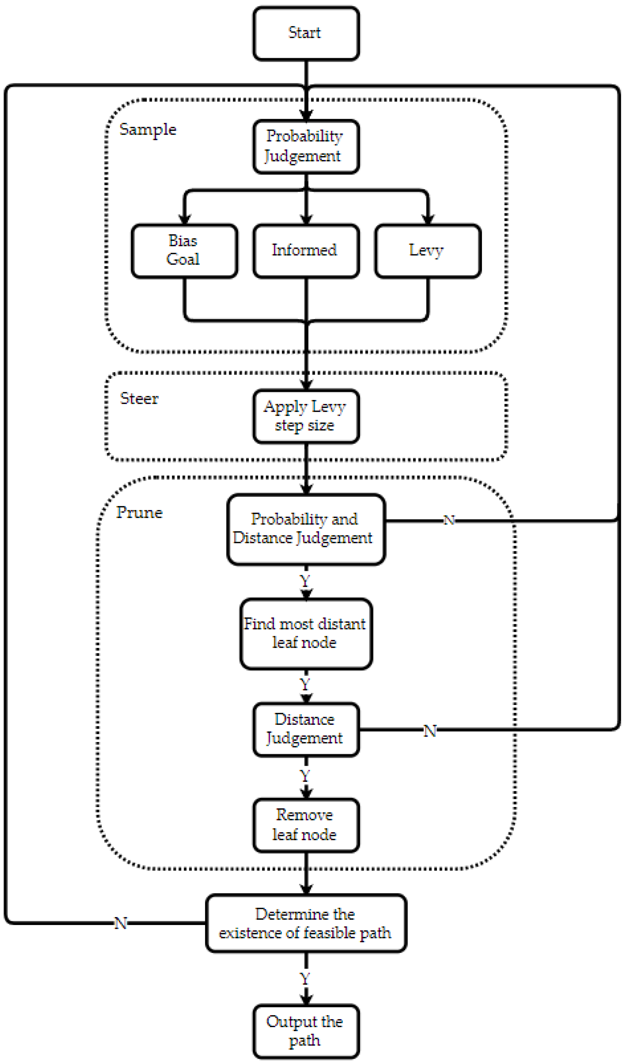
The traditional RRT* algorithm is characterized by slow convergence, blindness, and a tendency to become trapped in local optima. To address these shortcomings, HPS-RRT employs a hybrid sampling strategy that probabilistically selects from different sampling methods to balance their respective strengths and weaknesses. The sampling strategies utilized in HPS-RRT* are outlined in Table 2:
As shown in Table 2, each sampling strategy has its advantages and disadvantages.
The Bias-goal strategy includes a certain probability of directly selecting the goal point as a sample during the sampling process, allowing for a quicker approach to the target. However, this method is prone to becoming trapped in local optima and has lower search efficiency in complex and diverse environments.
Inspired by the Informed-RRT* algorithm, the Informed strategy narrows the sampling space during exploration. It focuses on the starting point n start and the node n close closest to the goal, constructing an ellipse with a semi-major axis of twice the distance between these two points. The sampling process within this ellipse is as follows:
  • Construct the ellipse based on n start and n close ;
  • Calculate the rotation angle θ of the ellipse using the following formula:
    θ = a r c t a n y close     y start x close     x start
Here,   x start and y start represent the axis value of n start , and x close and y close represent the axis value of n close .
3.
Sample within a horizontally oriented ellipse with the same semi-major and semi-minor axes as the constructed ellipse;
4.
Apply the rotation matrix to the sampled points matrix to rotate it into the constructed ellipse, resulting in the actual sampled point coordinates, as given by the following formula:
x new y new = cos θ sin θ sin θ cos θ x y
where x new y new represents the coordinates of the sampled points, cos θ sin θ sin θ cos θ is the corresponding rotation matrix, and x y denotes the coordinates of the points within the horizontal ellipse.
This sampling strategy utilizes a smaller, effective sampling space, improving search efficiency and optimizing the path. However, frequent computations can consume significant computational resources, placing certain demands on the processing platform. Additionally, the strategy exhibits poor adaptability in complex obstacle regions, making it challenging to find feasible paths.
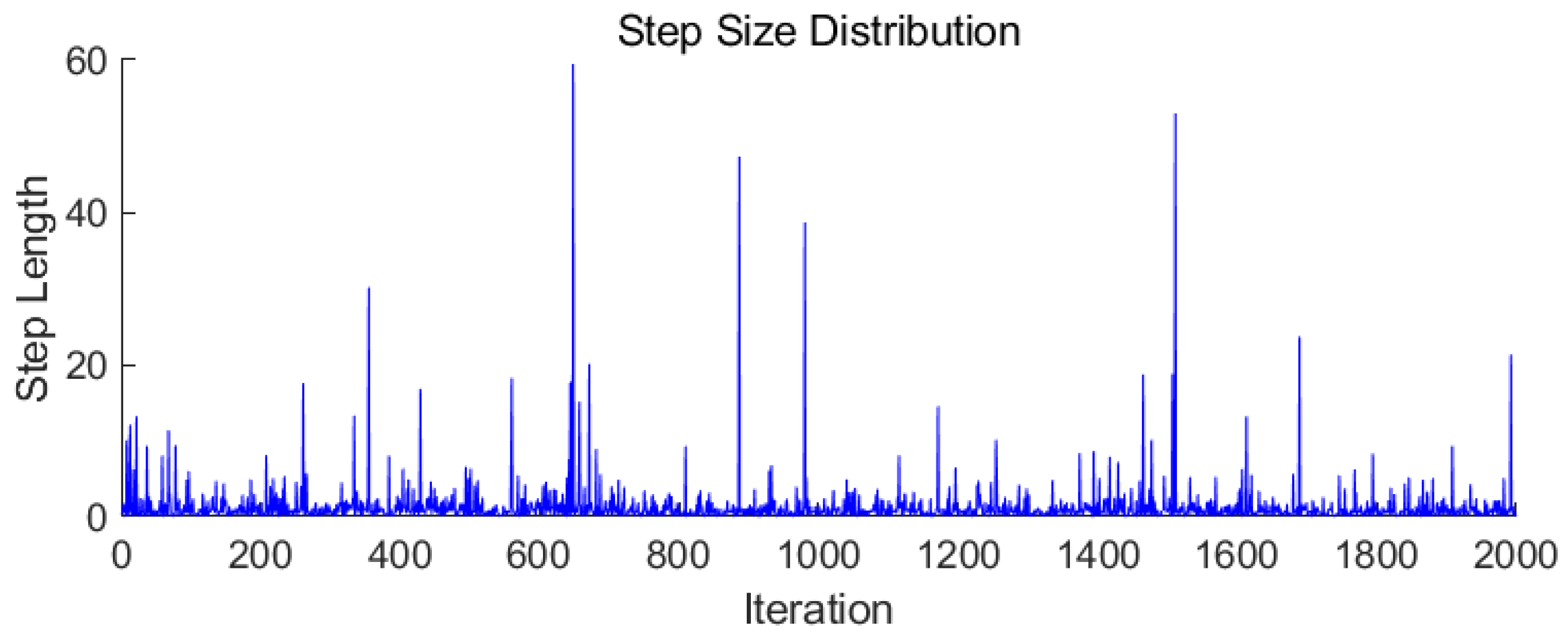
Lévy sampling is a sampling strategy that follows a Lévy distribution, characterized by its heavy-tailed probability distribution. In sampling, it manifests as frequent small-range samples interspersed with occasional large-range samples, a process known as the Lévy flight strategy. The sampling procedure is as follows:
  • Set the shape parameter β and the scaling factor α to calculate the Lévy step length s L . In a standard Lévy distribution, the formula for σ is as follows:
    s L = α     u v 1 β
    where u and v are random variables, with u ~ N ( 0 ,   σ 2 ) and v ~ N ( 0 ,   1 )   ( 0 , 1 ) . The formula for σ is as follows:
    σ = Γ 1 + β     sin π     β 2 β     Γ 1 + β 2 2 β     1 2 1 β
    Γ x = 0 t x 1     e t d t
  • Calculate the closest node to the target point, denoted as n close .
  • Using n close as the reference point, move a distance s L in a random direction D r to obtain the sample point n new . The formula is as follows:
    n new = n close + D r   s L
The Lévy sampling strategy enhances algorithm adaptability in complex environments through localized sampling. Additionally, occasional large-range sampling helps to mitigate local optima, improving global optimality; however, it exhibits poor performance in local optimization.
Each sampling strategy has its advantages and disadvantages. The HPS-RRT* algorithm balances these by probabilistically selecting different sampling strategies at each step, allowing it to enhance path quality and adaptability in complex environments while maintaining convergence speed.

3.2. Lévy Step Size

The traditional RRT* algorithm employs a fixed step size, leading to low node expansion efficiency and poor robustness across different maps, making parameter tuning challenging. This paper proposes using a Lévy step size, characterized by frequent small movements and occasional large jumps. The small movements facilitate navigation through complex environments, enhancing search efficiency, while the large jumps help to escape local optima, improving path quality. The Lévy step size enhances algorithm robustness while maintaining exploration efficiency, exhibiting low parameter sensitivity and high adaptability to various maps and environments. Its specific expression is given in Equation (3). The parameter β typically ranges from 1 to 2; closer to 1 indicates a stronger heavy-tailed Lévy distribution with a higher probability of long-distance jumps, enhancing global search capability. Conversely, closer to 2 results in a distribution similar to a Gaussian distribution, with smaller random step sizes and fewer long jumps, favoring local exploration. In this algorithm, β is set to 1.5, balancing local searches with adequate global search ability.
To visually observe the distribution of Lévy step lengths, we performed 2000 iterations based on the aforementioned formula, yielding the distribution shown in Figure 5.
In Figure 5, it is evident that the Lévy step length distribution consists of frequent small steps and occasional large steps. This characteristic aids in cautious node connections through complex obstacle-laden areas during exploration. Moreover, the occasional large steps can help escape local optima, enhancing exploration efficiency.

3.3. Leaf Prune

In the RRT* algorithm, each node connection is retained throughout the exploration process, which may lead to tree growth in incorrect or suboptimal directions. This can decrease exploration efficiency and increase the time required for path planning. To address this issue, HPS-RRT* introduces a pruning strategy inspired by ecological mechanisms in natural tree growth, such as apical dominance and lower branch degradation. This strategy aims to optimize the algorithm’s exploration and convergence performance. The specific process is outlined as follows:
  • When connecting a new node n new , if it is closer to the target than the nearest node n close , a pruning decision is initiated.
  • After meeting certain probabilistic criteria, the process proceeds, simulating the uncertainty in tree growth.
  • The farthest node from n new , labeled n distant , is identified, and the distance to n distant is calculated.
  • If this distance exceeds half of the direct distance from the start point to the target, the n distant node is eliminated, simulating the degradation or wilting of lower leaves.
This strategy ensures stable tree growth during the initial exploration phase, allowing for comprehensive expansion and preventing premature convergence to local optima. In the later stages, as the tree approaches the target point, the pruning mechanism gradually directs the tree toward the target, reducing ineffective branches and enhancing algorithm efficiency. By removing nodes that are distant from the target, unnecessary search areas can be effectively minimized, conserving computational resources. The resultant effect is illustrated in Figure 6.
In Figure 6, n new represents the new node, n close denotes the nearest point to the target before connecting the new node, n distant is the farthest node from n new , n start indicates the starting point, and n goal signifies the target point. Distances a and b correspond to the distances from n close and n new to the target, respectively. The circular shapes represent nodes, solid lines indicate actual connections, and dashed lines illustrate the pruning operation.
From the diagram, it can be observed that when b < a and the distance and probability criteria are satisfied, a pruning operation is performed. The farthest node n distant from n new and its connecting segments are pruned, as indicated by the dashed lines in Figure 6.
This visually demonstrates that the overall trend of the tree after pruning is more aligned with the target point, akin to the growth of terminal buds in branches. This improvement enhances the convergence rate during node expansion, directing the expansion closer to the target point and reducing the exploration of erroneous directions.

3.4. Leader-Based Sparrow Optimization Algorithm

Conventional RRT or RRT* algorithms often yield paths that are unsuitable for tracking by tracked robots in orchards. Some paths exhibit large curvature, failing to meet the maximum turning radius requirements of the tracked robots, which hinders effective tracking performance. Additionally, the generated paths are typically excessively long and not globally optimal, leading to increased operational costs and reduced efficiency for agricultural robots. This paper proposes an optimization strategy based on vehicle kinematic constraints—the improved sparrow search algorithm—to address this issue.
The sparrow search algorithm, as a heuristic swarm intelligence optimization method, is widely applied in various optimization scenarios. Its core idea is to simulate the foraging and anti-predation behaviors of sparrows, leveraging the collaboration and division of labor among individual members of the population to achieve effective global search and avoid local optima. In the conventional sparrow search algorithm, there are typically two roles: foragers and followers. Foragers are responsible for approaching the global optimum and enhancing solution diversity through random searches, simulating the foraging process of sparrows. On the other hand, followers focus on tracking the optimal solution while escaping from the worst solution, mimicking the anti-predation behavior and cooperative functionality of sparrows [29]. The sparrow search algorithm is characterized by strong global search capability, fast convergence speed, and fewer parameters that are easy to adjust. The general procedure is as follows:
  • Initialize the sparrow population;
  • Assign roles to the sparrows;
  • Execute functions based on assigned roles;
  • Calculate fitness and update the optimal solution;
  • Check if the maximum iteration count is reached; if so, output the optimal solution; otherwise, return to step 3 for further iterations.
In path optimization, two key metrics require significant attention: the maximum curvature (or smoothness) of the path, which affects its suitability for actual navigation tasks and is critical for the tracking performance of the robot, and the path length, where shorter paths can reduce navigation time costs and enhance operational efficiency. In conventional sparrow search algorithm implementations, optimizing both maximum curvature and path length simultaneously may lead to paths with a greater maximum curvature after optimization compared to before. Additionally, while traditional path smoothing algorithms, such as B-spline optimization, can create smoother paths, they often overlook changes in path length, potentially resulting in an optimized path that is longer than the original. To comprehensively consider the two performance metrics mentioned above, ensuring that the maximum curvature of the path meets the robot’s movement requirements while achieving a shorter and safer path, HPS-RRT* employs an improved sparrow search algorithm.
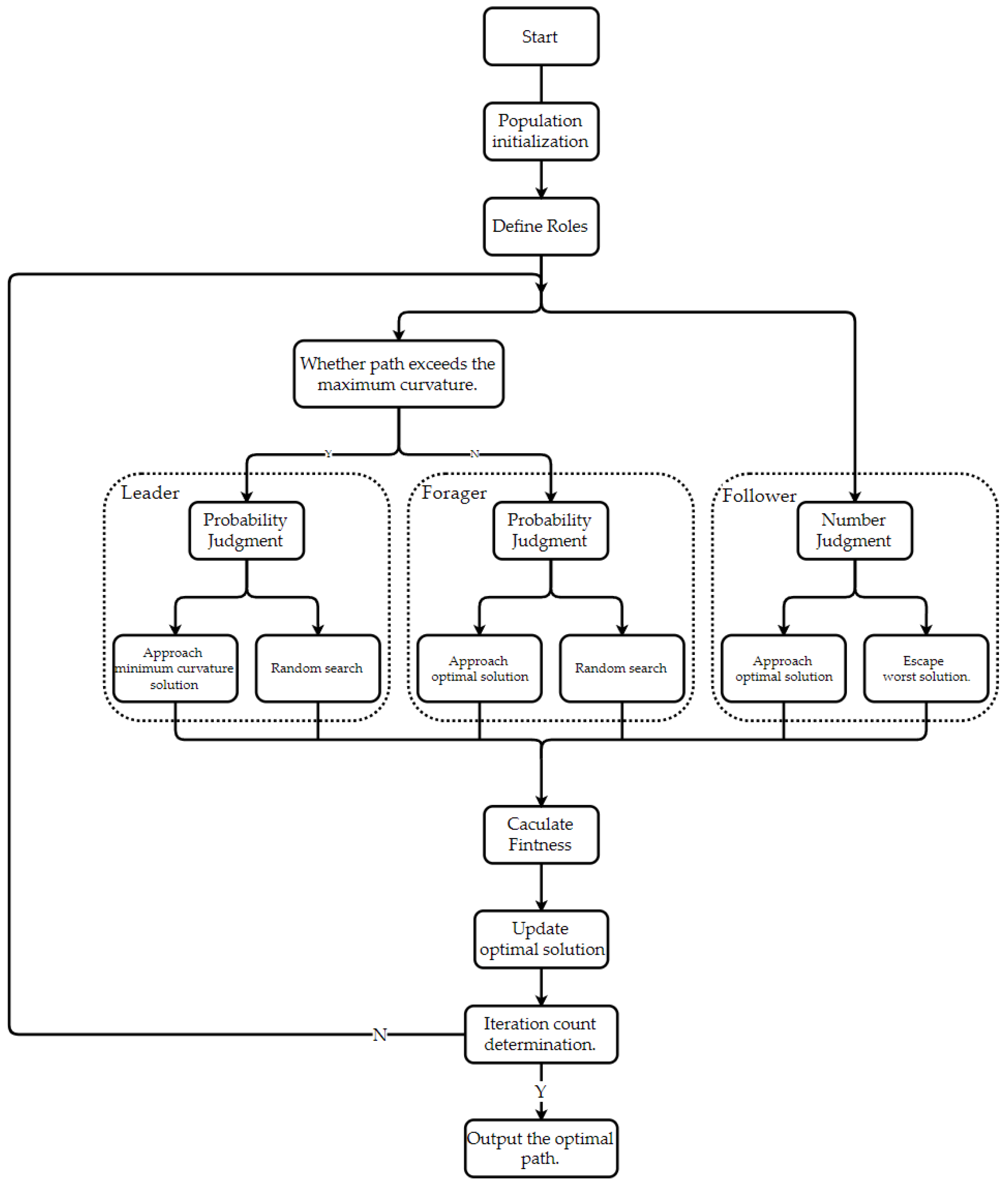
The HPS-RRT* algorithm integrates and enhances the sparrow search algorithm for path optimization by innovatively proposing a leader-based sparrow optimization algorithm. This approach aims to optimize curvature while ensuring path optimality. The optimization process is shown in Figure 7:
At the beginning of the optimization loop, the sparrow optimization algorithm calculates the fitness value based on the current path length and maximum curvature. The formula is as follows:
F i t n e s s =   α 1 L +   α 2 C u r
where α 1 and α 2 represent the penalty weights, L denotes the path length, and Cur indicates the maximum curvature of the path.
Next, a population of sparrows is randomly initialized, where this initialization involves applying random perturbations to the control points of the existing path. This process yields sparrows with diverse solutions, which are then categorized into different roles proportionally.
During each optimization iteration, the algorithm checks whether the current path meets the maximum curvature constraint to ensure feasibility. If the constraint is not satisfied, the leader mechanism is triggered. In this case, the leader assumes the role of the forager with a certain probability, guiding the population towards the solution with minimal curvature or conducting a random search.
The adjustment of control points in the path optimization can be expressed by the following formula:
P x new , y new = P x old , y old + s rand   D min , p < 0.7 P x old , y old + s rand   D rand , p 0.7
In this context, P ( x old , y old ) represents the original control points, while P ( x new , y new )   denotes the optimized control points. The parameter s rand is a random number between 0 and 1, which should be adjusted according to the size of the map and the path. D min indicates the direction of the solution with the minimum curvature and D rand represents a random direction. Finally, p is a random probability between 0 and 1.
The leader mechanism effectively reduces the maximum curvature of the path, enhances path smoothness, and maintains solution diversity during the optimization process, thereby preventing convergence to local optima.
If the path satisfies the constraints, the forager will converge towards the optimal solution with a certain probability or explore in a random direction. This can be expressed by the following formula:
P x new , y new = P x old , y old + s rand D opt , p < 0.7 P x old , y old + s rand D rand , p 0.7
Here, P ( x o l d , y o l d ) represents the original control points, and P ( x new , y new ) denotes the optimized control points. s rand is a random number between 0 and 1, D best indicates the direction of the current optimal solution, D rand represents a random direction, and p is a random probability between 0 and 1.
The forager’s search allows the population to explore to a certain extent while simultaneously seeking the optimal solution, thereby enhancing the diversity of solutions.
The followers will either converge toward the optimal solution or evade danger by moving away from the worst solution. This can be expressed by the following formula:
P x new , y new = P x old , y old +   s rand D best , p < 0.5 P x old , y old + s rand D worst , p 0.5
Here, P ( x old , y old ) represents the original control points, while P ( x new , y new ) denotes the optimized control points. s rand is a random number between 0 and 1, s rand indicates the direction of the current optimal solution, D worst represents the direction to escape from the worst solution, and p is a random probability between 0 and 1.
The followers are responsible for maintaining the stability of the population’s trend, with half of them approaching the optimal solution and the other half escaping the worst solution. This leads to an overall improvement in the population’s direction.
At the end of each iteration, the fitness of each sparrow in the population is calculated, and the optimal and worst solutions are updated, continuing until the maximum number of iterations is reached.
The final optimized path obtained through the above optimization process achieves optimality while satisfying curvature constraints. The sparrow optimization algorithm demonstrates significant advantages in convergence speed and global optimization compared to traditional algorithms such as SA and PSO. Additionally, the improved sparrow optimization algorithm features a prioritized optimization process that allows for flexible expansion and differentiated optimization of various path characteristics to meet diverse path requirements.
This algorithm has significant advantages over traditional path smoothing optimization methods, such as B-spline optimization, which often struggles to balance path length requirements and safety, leading to higher collision risks with obstacles. The improved sparrow optimization algorithm effectively addresses this issue by simultaneously optimizing path smoothness and globally optimizing path length to achieve an overall optimal solution.

4. Results and Discussion

To demonstrate the superiority of the HPS-RRT* algorithm, Map1, Map2, and Map3, as shown in Figure 8, were utilized as simulation maps of different complexity. Each map measures 1000 × 1000 and simulates different environments to assess the algorithm’s performance in complex scenarios.
In Figure 8, the white areas represent navigable regions, while the black areas indicate obstacles.
This experiment compares four algorithms: RRT*, Bias-RRT*, Connected-RRT*, and PRM*, with identical parameters across different maps. The parameters of the HPS-RRT* algorithm are shown in Table 3 and remain consistent in all subsequent experiments.
Bias-RRT* improves the traditional RRT by incorporating a fixed target-biased sampling probability, enhancing the likelihood of sampling near the target node. This approach accelerates the convergence by directly selecting the target node as a sampling point with a certain probability during random node generation, thereby expediting the path discovery process. Connected-RRT*, on the other hand, adopts a bidirectional strategy, simultaneously extending node trees from both the start and the goal points. This bidirectional expansion facilitates quicker connections between the two trees, significantly reducing path search time. PRM* differs from the RRT* algorithm in its planning process. It randomly distributes a certain number of nodes within the map and attempts to connect each node with others. If the distance between nodes is within a predefined range, the connection is considered valid; otherwise, it is discarded. Dijkstra’s algorithm is then employed to find the optimal trajectory, with the resulting path chosen as the final output. As a graph-based search algorithm, PRM* is applicable to high-dimensional spaces. However, its efficiency decreases significantly in environments with narrow passages or dense obstacles, and it may even fail to find a solution under such conditions.

4.1. Comparison of Map Performance

Figure 9, Figure 10 and Figure 11 illustrate the performance of different algorithms on various maps. Green or blue line segments represent the expansion tree’s attempted paths, while the red line segment indicates the final actual path. The red triangle marks the starting point, the blue triangle marks the goal, and the black regions represent obstacle areas.
A comparison of the different results shows that HPS-RRT* achieves faster convergence, with the shortest and smoother final paths, making it more suitable for trajectory tracking of the orchard crawler robot.
The performance comparison of different algorithms on various maps is presented in Table 4.
Here, “ALength” represents the average length of the effective paths discovered, “ATime” refers to the computation time from the start to the end of exploration to evaluate the algorithm’s convergence performance, “SRate” indicates the average success rate of exploration, where success is defined as planning a collision-free path to the target point, and “ACur” refers to the mean maximum curvature, used to evaluate path smoothness.
As shown in Table 4, HPS-RRT* consistently demonstrates superior performance across various environments. Compared to RRT*, Bias-RRT*, and Connect-RRT*, it achieves improvements in path length by approximately 1.7%, 2.2%, and 27.0%, respectively, as well as in planning time by approximately 93.3%, 86.4%, and 77.7%. Moreover, HPS-RRT* consistently achieves a 100% success rate. In comparison with PRM*, while HPS-RRT* may have slightly higher planning times in certain maps, its path length is improved by approximately 3.1%. Additionally, HPS-RRT* shows significant enhancements in smoothness compared to all four algorithms, with improvements of approximately 27.9%, 39.7%, 39.0%, and 41.7% over PRM*, RRT*, Bias-RRT*, and Connect-RRT*, respectively.
To further validate the superiority of the HPS-RRT* algorithm, paired sample T-tests were conducted to compare its performance with RRT*, Bias-RRT*, Connected-RRT*, and PRM*, verifying the differences in various performance metrics.
The paired sample T-test, widely used in statistics to compare the means of two related samples, involves the following steps:
  • Perform a normality test: Verify that the samples follow a normal distribution; if satisfied, proceed to the next step;
  • Set the hypotheses: Define the null hypothesis H 0 ; the means of the two related samples are equal, indicating no difference. In the alternative hypothesis H 1 , the means of the two samples are not equal, indicating a difference;
  • Calculate the means and standard deviations: Use the following formulas for mean d - and standard deviation s d :
    d - = 1 n i = 1 n d i
    s d = 1 n     1 i = 1 n d i   d - 2
    where d i represents sample differences and n is the sample size.
  • Compute the T-value t and degrees of freedom d f ;
    t = d - s d / n
    d f = n 1
    where d - is the mean of differences, s d is the standard deviation, and n is the sample size.
  • Determine the p-Value: Based on the computed t and d f , find the corresponding p from the t-distribution table.
  • Compare with the significance level: If p   <   α (commonly 0.05), reject the null hypothesis H 0 , concluding a significant difference in means; otherwise, accept H 1 .
To quantify the magnitude of differences, Cohen’s d is introduced, and calculated as follows:
d = y 1 ¯     y 2 ¯ σ pooled
σ pooled = n 1   1 s 1 + n 2   1 s 2 n 1 + n 2 1 2
where y 1 ¯ and y 2 ¯ are sample means, s 1 and s 2 are standard deviations, and n 1 and n 2 are sample sizes.
The algorithm result data were subjected to normality tests, and all sample data passed the normality requirement. The null hypothesis H 0 was set as follows: the means of the two related samples are equal, indicating no difference. The alternative hypothesis H 1 was set as follows: the means of the two samples are not equal, indicating a significant difference. A significance level of p = 0.05 was chosen. Paired sample T-tests were conducted to compare the path length, planning time, and the maximum curvature of HPS-RRT* with RRT*, Bias-RRT*, Connect-RRT*, and PRM*. The results of the comparisons between each algorithm with HPS-RRT* are shown in Table 5.
A Cohen’s d value less than 0.2 indicates a negligible effect size, values in the range [0.2, 0.5) indicate a small effect size, and values greater than 0.8 indicate a large effect size. As shown in Table 5, most Cohen’s d values for HPS-RRT* compared to other algorithms are greater than 0.5. This indicates that the mean performance of HPS-RRT* is significantly different from, and substantially better than, the compared algorithms.
The HPS-RRT* algorithm employs a hybrid sampling strategy and a Lévy distribution step size optimized through a pruning strategy to significantly enhance the search speed for paths. Utilizing a leader-based sparrow optimization algorithm ensures that the paths not only meet the maximum curvature requirements of the robot but also minimize path length, achieving a global optimum. The experimental results demonstrate that the HPS-RRT* algorithm converges quickly, generates high-quality planned paths, and shows excellent adaptability to complex environments, outperforming the comparison algorithms and significantly exceeding the performance of traditional RRT* algorithms.

4.2. Experiment on Multi-Target Point Map in Orchard

To validate the effectiveness of the algorithm in orchard environments, the tracked robot shown in Figure 12 was employed for mapping. This robot is equipped with a MID360 LiDAR and a high-precision IMU for mapping and real-time localization. Additionally, it features a dual-line GPS system, enabling high-precision positioning for future experiments. The detailed kinematic parameters of this tracked robot are listed in Table 6.
Based on the kinematic parameters of the tracked robot, the maximum wheel speed of the left and right tracks is 6 km/h, and the wheelbase is 290 mm. Assuming the robot performs a maximum radius turn where one track remains stationary and the other moves at maximum speed, the kinematic modeling is as follows:
To adapt to the complex terrain of agricultural environments such as orchards, this paper utilizes a tracked two-wheel robot model, which can also be regarded as a differential-drive robot. Its motion is determined by two independently controlled tracks. The simplified model of the tracked two-wheel robot chassis is shown in Figure 13:
Here, L represents the track spacing (distance between the two tracks), V L and V R are the linear velocities of the left and right tracks, respectively, and θ denotes the robot’s heading angle. B represents the robot’s center, ω is the angular velocity, and V denotes the linear velocity of the robot’s center. The calculations yield the following relationships:
The center velocity V and angular velocity ω are as follows:
V = V L + V R 2
ω = V R     V L L
The turning radius R and steering curvature k are as follows:
R = V ω = L V L + V R 2 V R     V L
k = ω V = 2 V R     V L L V L + V R
Additionally, the robot’s pose is updated in real-time using the following equations:
x   ˙ = V   cos θ
y ˙ = V   sin θ
θ ˙ = ω
According to Equations (17)–(20), the maximum steering curvature is 2.341 m−1.
The mapping site is a pomelo orchard, with the arrangement of the trees illustrated in Figure 14. Figure 15 presents the 3D point cloud of the orchard.
In Figure 15, the colors correspond to the color bar on the right, representing the Z-axis data from smallest to largest, where the minimum value is 0 and the maximum is 2 m.
To ensure the planning results are clear and intuitive, the local part of the 3D point cloud data is dimensionally reduced and converted into a grid map. Regions with a Z-axis height greater than 0.1 m are defined as obstacles, as shown in Figure 16a. Additionally, to accommodate the actual volume of the orchard robot, obstacle expansion was applied, which expanded the volume of the obstacles to 2.5 times the original size, as illustrated in Figure 16b.
In Figure 16, the white areas represent navigable regions, while the black areas indicate obstacles.
In the experiment, a series of target points were preset to simulate the path points required for actual fruit tree harvesting. Multi-objective planning was then performed sequentially based on these target points, as shown in Figure 17.
In Figure 17, the green triangle represents the starting point, the blue triangle indicates the endpoint, the red triangles are path points, the black objects are obstacles, the green line segments show the exploration path, and the blue curve represents the actual path.
After conducting 100 experiments, the average maximum curvature of the final path was calculated as 0.35 m−1, which is smaller than the tracked robot’s maximum curvature of 2.341 m−1, meeting its kinematic requirements. The final path was smooth, continuous, and collision-free, making it directly applicable to navigation in actual orchard operations. In all 100 experiments, HPS-RRT* successfully planned the path, demonstrating its robust performance in large, unstructured maps such as orchards. Additionally, the standard deviation of the maximum curvature is 0.1158, and the average planning time is 7.51 s.
To further evaluate the superiority of the HPS-RRT* planned path in practical navigation, a trajectory-tracking control experiment was designed based on the kinematic model of the orchard robot. The final results are shown in Figure 18.
In Figure 18, the green triangle represents the starting point, the blue triangle indicates the endpoint, the blue dashed line denotes the reference path, and the red solid line represents the tracked trajectory.
The figure intuitively shows that the tracked trajectory aligns well with the reference path, achieving a path overlap rate of 97.78%. This demonstrates that the path meets the practical navigation requirements of the orchard robot.

4.3. Robustness and Sensitivity Analysis of the Algorithm

Map3 is used as the baseline map to evaluate the algorithm’s robustness and to conduct 100 experiments intuitively and effectively. In each experiment, 25 randomly sized obstacles are introduced as external disturbances to test the algorithm’s performance under such conditions. The approximate planned paths are illustrated in Figure 19.
In Figure 19, the red line represents the planned path, the red triangle denotes the starting point, the blue triangle indicates the goal point, the black areas represent obstacles, and the white areas indicate feasible regions.
The performance metrics are summarized in Table 7, where “Basis” represents the baseline map and “Interference” represents the map with added disturbances.
From Table 7, it can be observed that under certain external disturbances, the performance metrics of HPS-RRT* show minimal variations compared to the baseline. This demonstrates the strong robustness of the HPS-RRT* algorithm.
To further evaluate the sensitivity of various parameters in the HPS-RRT* algorithm, Map3 was selected as the experimental map. The experiments were conducted 100 times for four groups of algorithm parameters: A, B, C, and D. The specific parameters for A, B, C, and D are detailed in Table 8.
The experimental results are shown in Table 9, where “Basis” represents the original parameters.
As shown in Table 9, the impact on “Length” under different parameters ranges from approximately 0.04% to 1.2%, indicating a minimal effect. The impact on “Time” ranges from about 0.7% to 52.0%, showing a significant effect, while the impact on “Curvature” is around 16.7% to 40.7%, which is relatively small.
Thus, it can be concluded that adjusting the parameters of HPS-RRT* has a considerable effect on planning time. Different parameters should be selected for different maps to enhance planning efficiency, further demonstrating that HPS-RRT* is highly sensitive to parameter settings and requires careful selection to adapt to various environments.

5. Conclusions

To address the issues of low success rates, inefficient searches, poor path quality, and insufficient smoothness in existing path planning algorithms for unstructured environments like orchards, this study proposes the HPS-RRT* algorithm. To counter the low planning efficiency caused by the random sampling strategy in traditional RRT algorithms, a hybrid sampling strategy is employed, significantly improving planning speed and reducing ineffective sampling points. The HPS-RRT* algorithm utilizes an extended step size based on Lévy distribution to ensure both the efficiency and quality of the planned paths, thereby resolving the inefficiencies, rigidity, and collision issues associated with fixed step sizes. Additionally, to tackle the redundancy of ineffective nodes during the planning process, an innovative pruning strategy is introduced to eliminate redundant nodes during tree growth, enhancing search efficiency. To improve the smoothness of the final paths generated by traditional RRT algorithms, the proposed method incorporates a leader-based sparrow optimization algorithm, which optimizes both path curvature and length, allowing for direct application in path tracking.
The experimental results indicate that the proposed HPS-RRT* algorithm outperforms RRT, Bias-RRT*, Connect-RRT, and PRM algorithms in several aspects. The final path length was reduced by 1.7% to 27%, planning efficiency improved by 77.7% to 93.3%, and path smoothness increased by approximately 27.9% to 41.7%, achieving a success rate of 100%, while other algorithms occasionally experienced planning failures. The calculated average maximum curvature of the paths was 0.8 m−1, confirming the feasibility of the HPS-RRT* algorithm for robotic applications in orchard environments.
In conclusion, the proposed HPS-RRT* algorithm effectively addresses path planning issues in unstructured environments such as orchards. However, it remains sensitive to parameter selection, making appropriate parameter tuning crucial across different map scenarios. Additionally, the HPS-RRT* algorithm has only been tested in static environments, lacking adaptability to dynamic scenarios. The experimental results also indicate that HPS-RRT* has high computational demands and relies on hardware performance, which may affect its application in real-time navigation.
In future work, we will attempt to utilize neural network algorithms such as reinforcement learning to optimize the sampling strategy’s probabilities, enabling dynamic adjustments for different environments. Additionally, the algorithm will be extended to incorporate real-time dynamic obstacle avoidance by integrating predictive models or local obstacle avoidance strategies. Furthermore, we aim to explore the practical performance of HPS-RRT* across various hardware platforms, optimizing its operational efficiency.

Author Contributions

Conceptualization, M.H. and Q.H.; methodology, M.H. and J.C.; software, M.H.; validation, Q.H. and Y.C.; formal analysis, J.L. and L.S.; investigation, M.H. and Q.H.; resources, M.H. and Q.H.; data curation, M.H. and J.C.; writing—original draft preparation, M.H. and Q.H.; writing—review and editing, L.S.; visualization, M.H. and J.C.; supervision, Y.C. and J.L.; funding acquisition, L.S. All authors have read and agreed to the published version of the manuscript.

Funding

This work was supported by the Guangdong Basic and Applied Basic Research Foundation under Grant 2024A1515010135, the National Natural Science Foundation of China under Grant 62303188, and the 2024 Basic and Applied Research Project of Guangzhou Science and Technology Plan under Grant 2024A04J4140.

Institutional Review Board Statement

Not applicable.

Data Availability Statement

Data are contained within the article.

Conflicts of Interest

The authors declare no conflicts of interest.

References

  1. Duan, Z.; Qiu, W.; Ding, W.; Liu, Y.; Ouyang, Y. Tilting stability analysis and experiment of the 3-DOF lifting platform for hilly orchards. Int. J. Agric. Biol. Eng. 2018, 11, 73–80. [Google Scholar] [CrossRef]
  2. Zhang, M.; Li, X.; Wang, L.; Jin, L.; Wang, S. A Path Planning System for Orchard Mower Based on Improved A* Algorithm. Agronomy 2024, 14, 391. [Google Scholar] [CrossRef]
  3. Liu, L.; Liu, H.; Li, J.; Wang, P.; Yang, X. Construction of Orchard Agricultural Machinery Dispatching Model Based on Improved Beetle Optimization Algorithm. Agronomy 2025, 15, 323. [Google Scholar] [CrossRef]
  4. Chen, B.; Quan, G. NP-Hard Problems of Learning from Examples. In Proceedings of the 2008 Fifth International Conference on Fuzzy Systems and Knowledge Discovery, Jinan, China, 18–20 October 2008; Volume 2, pp. 182–186. [Google Scholar]
  5. Karur, K.; Sharma, N.; Dharmatti, C.; Siegel, J.E. A Survey of Path Planning Algorithms for Mobile Robots. Vehicles 2021, 3, 448–468. [Google Scholar] [CrossRef]
  6. Kun, S.; Yang, L.; Wu, Z.; Jiang, B.; Gao, Q. Multi-robot dynamic path planning with priority based on simulated annealing. J. Frankl. Inst. 2025, 362, 107396. [Google Scholar]
  7. Wang, S.; Zhao, T.; Li, W. Mobile Robot Path Planning Based on Improved Artificial Potential Field Method. In Proceedings of the 2018 IEEE International Conference of Intelligent Robotic and Control Engineering (IRCE), Lanzhou, China, 24–27 August 2018; pp. 29–33. [Google Scholar]
  8. El-Teleity, S.A.L.; Nossair, Z.B.; Mansour, H.M.A.K. Fuzzy logic control of an autonomous mobile robot. In Proceedings of the 2011 16th International Conference on Methods & Models in Automation & Robotics, Miedzyzdroje, Poland, 22–25 August 2011; pp. 188–193. [Google Scholar]
  9. Zhu, Y.; Zhang, G.; Chu, R.; Xiao, H.; Yang, Y.; Wu, X. Research on escape route planning analysis in forest fire scenes based on the improved A* algorithm. Ecol. Indic. 2024, 166, 112355. [Google Scholar] [CrossRef]
  10. Ajeil, F.H.; Ibraheem, I.K.; Azar, A.T.; Humaidi, A.J. Grid-Based Mobile Robot Path Planning Using Aging-Based Ant Colony Optimization Algorithm in Static and Dynamic Environments. Sensors 2020, 20, 1880. [Google Scholar] [CrossRef]
  11. Gong, P.; Li, W.; Ma, Q.; Hu, W. Research on Path Planning for Unmanned Vehicles Based on Improved A* Algorithm. J. Combin. Machine Tools Autom. Process 2023, 3, 17–20,24. [Google Scholar]
  12. Kazemi, M.; Gupta, K.K.; Mehrandezh, M. Randomized Kinodynamic Planning for Robust Visual Servoing. IEEE Trans. Robot. 2013, 29, 1197–1211. [Google Scholar] [CrossRef]
  13. Kavraki, L.E.; Svestka, P.; Latombe, J.C.; Overmars, M.H. Probabilistic roadmaps for path planning in high-dimensional configuration spaces. IEEE Trans. Robot. Autom. 1996, 12, 566–580. [Google Scholar] [CrossRef]
  14. Liu, H.; Zhang, X.; Wen, J.; Wang, R.; Chen, X. Goal-biased Bidirectional RRT based on Curve-smoothing. IFAC-PapersOnLine 2019, 52, 255–260. [Google Scholar] [CrossRef]
  15. LaValle, S.M.; Kuffner, J.J., Jr. Randomized kinodynamic planning. Int. J. Robot. Res. 2001, 20, 378–400. [Google Scholar] [CrossRef]
  16. Karaman, S.; Frazzoli, E. Sampling-based algorithms for optimal motion planning with deterministic μ-calculus specifications. In Proceedings of the 2012 American Control Conference (ACC), Montreal, QC, Canada, 27–29 June 2012; pp. 735–742. [Google Scholar]
  17. Ye, L.; Li, J.; Li, P. Improving path planning for mobile robots in complex orchard environments: The continuous bidirectional Quick-RRT* algorithm. Front. Plant Sci. 2024, 15, 1337638. [Google Scholar] [CrossRef]
  18. Ye, L.; Wu, F.; Zou, X.; Li, J. Path planning for mobile robots in unstructured orchard environments: An improved kinematically constrained bi-directional RRT approach. Comput. Electron. Agric. 2023, 215, 108453. [Google Scholar] [CrossRef]
  19. Li, Y.; Zhao, J.; Chen, Z.; Xiong, G.; Liu, S. A Robot Path Planning Method Based on Improved Genetic Algorithm and Improved Dynamic Window Approach. Sustainability 2023, 15, 4656. [Google Scholar] [CrossRef]
  20. Zhu, A.; Yang, S. A Neural Network Approach to Dynamic Task Assignment of Multirobots. IEEE Trans. Neural Netw. 2006, 17, 1278–1287. [Google Scholar]
  21. Rashid, R.; Perumal, N.; Elamvazuthi, I.; Tageldeen, M.K.; Khan, M.A.; Parasuraman, S. Mobile robot path planning using Ant Colony Optimization. In Proceedings of the 2016 2nd IEEE International Symposium on Robotics and Manufacturing Automation (ROMA), Ipoh, Malaysia, 25–27 September 2016; pp. 1–6. [Google Scholar]
  22. Zheng, L.; Yu, W.; Li, G.; Qin, G.; Luo, Y. Particle Swarm Algorithm Path-Planning Method for Mobile Robots Based on Artificial Potential Fields. Sensors 2023, 23, 6082. [Google Scholar] [CrossRef]
  23. Rickert, M.; Sieverling, A.; Brock, O. Balancing Exploration and Exploitation in Sampling-Based Motion Planning. IEEE Trans. Robot. 2014, 30, 1305–1317. [Google Scholar] [CrossRef]
  24. Gammell, J.D.; Srinivasa, S.S.; Barfoot, T.D. Informed RRT*: Optimal sampling-based path planning focused via direct sampling of an admissible ellipsoidal heuristic. In Proceedings of the 2014 IEEE/RSJ International Conference on Intelligent Robots and Systems, Chicago, IL, USA, 14–18 September 2014; pp. 2997–3004. [Google Scholar]
  25. Kong, F.; Liu, B.; Han, X.; Yi, L.; Sun, H.; Liu, J.; Liu, L.; Lan, Y. Path Planning Algorithm of Orchard Fertilization Robot Based on Multi-Constrained Bessel Curve. Agriculture 2024, 14, 979. [Google Scholar] [CrossRef]
  26. Ben Hazem, Z. Study of Q-learning and deep Q-network learning control for a rotary inverted pendulum system. Discov. Appl. Sci. 2024, 6, 49. [Google Scholar] [CrossRef]
  27. Cui, J.; Nie, G. Motion Route Planning and Obstacle Avoidance Method for Mobile Robot Based on Deep Learning. J. Electr. Comput. Eng. 2022, 2022, 5739765. [Google Scholar] [CrossRef]
  28. Tsallis, C. Lévy distributions. Phys. World 1997, 10, 42. [Google Scholar] [CrossRef]
  29. Xue, J.; Shen, B. A novel swarm intelligence optimization approach: Sparrow search algorithm. Syst. Sci. Control Eng. 2020, 8, 22–34. [Google Scholar] [CrossRef]
Figure 1. RRT algorithm principle diagram.
Agronomy 15 00712 g001
Figure 2. RRT reconnection.
Agronomy 15 00712 g002
Figure 3. RRT optimization.
Agronomy 15 00712 g003
Figure 4. Flowchart of the HPS-RRT* algorithm.
Agronomy 15 00712 g004
Figure 5. Lévy Step Size Distribution.
Agronomy 15 00712 g005
Figure 6. Pruning effect diagram. (a and b indicate the distance between the corresponding two nodes).
Agronomy 15 00712 g006
Figure 7. Flowchart of the leader-based sparrow optimization algorithm.
Agronomy 15 00712 g007
Figure 8. Illustrative diagram of experimental maps: (a) Map1; (b) Map2; (c) Map3.
Agronomy 15 00712 g008
Figure 9. Path planning visualization for Map1: (a) HPS-RRT*; (b) PRM*; (c) RRT*; (d) Bias-RRT*; (e) Connected-RRT*.
Agronomy 15 00712 g009
Figure 10. Path planning visualization for Map2: (a) HPS-RRT*; (b) PRM*; (c) RRT*; (d) Bias-RRT*; (e) Connected-RRT*.
Agronomy 15 00712 g010
Figure 11. Path planning visualization for Map3: (a) HPS-RRT*; (b) PRM*; (c) RRT*; (d) Bias-RRT*; (e) Connected-RRT*.
Agronomy 15 00712 g011
Figure 12. The nonholonomic orchard robot.
Agronomy 15 00712 g012
Figure 13. Simplified model of the tracked two-wheel robot chassis.
Agronomy 15 00712 g013
Figure 14. Actual environment of the orchard.
Agronomy 15 00712 g014
Figure 15. Three-dimensional point cloud of orchard.
Agronomy 15 00712 g015
Figure 16. Two-dimensional map of orchard. (a) Before expansion; (b) after expansion.
Agronomy 15 00712 g016
Figure 17. Orchard planning map.
Agronomy 15 00712 g017
Figure 18. Trajectory tracking performance diagram.
Agronomy 15 00712 g018
Figure 19. Path diagram.
Agronomy 15 00712 g019
Table 1. The characteristics and limitations of various path planning algorithms.
AlgorithmsCharacteristicsLimitationsReference Index
Simulated annealingThe annealing process in physics, avoids local optimaSlow convergence, challenging parameter tuning[6]
Artificial potential field methodAttractive source, repulsive source, strong real-timePath lacks smoothness, oscillation, local optima[7]
Fuzzy control methodAdaptation to nonlinear systemsDesigning fuzzy rules requires expertise[8]
A* algorithmHeuristic function, static environment, shortest pathPoor path smoothness, excessive turning points[9]
Grid-based methodStatic obstacle environment with grid discretizationPoor path smoothness, low path quality, efficiency[10]
RRTRapidly exploring random trees, real-time path updatePoor path smoothness, challenging parameter tuning[12]
PRMGraph-based search algorithm, high-dimensional spaceNot well-suited for narrow environments[13]
Genetic algorithmSimulates natural selection and genetic variationPremature convergence, slow convergence[17]
Artificial neural networkData training, pattern recognition, decision-makingRequires large training data, low interpretability[18]
Ant colony algorithmAnt foraging, pheromoneSlow convergence, local optima[19]
Particle swarm optimizationBird foraging, information sharing among particlesChallenging parameter tuning[20]
EETExtended tree, adaptable to dynamic environmentsHighly complex with extensive algorithmic details[21]
Deep learningFeature extraction, large-scale real-time decision-makingNeeds extensive labeled data, poor model interpretability[24]
Table 2. Hybrid sampling strategy.
MethodProbabilityAdvantageDisadvantage
Bias-goal0.2Fast convergence to the goalRisk of local minima
Informed0.4Efficient optimizationHigh computation cost
Lévy0.4Strong global explorationWeak path optimization
Table 3. HPS-RRT* parameter table.
ParametersSymbolValue
Step gain coefficient α 100
Lévy shaping parameter β 1.5
Initial population size of sparrows ε 30
Number of iterations in the sparrow i 1000
Table 4. Comparison of data across different maps.
MethodMap1Map2Map3
ALengthATimeSRateACurALengthATimeSRateACurALengthATimeSRateACur
HPS-RRT*1376.980.19100%0.101489.832.20100%0.101376.550.24100%0.08
PRM*1410.120.3198%0.121533.250.1891.00%0.141437.110.13100%0.13
RRT*1399.805.68100%0.171520.4817.3052.000.181398.445.79100%0.12
Bias-RRT*1408.662.91100%0.171535.688.9358%0.161398.962.57100%0.13
Connect-RRT*1873.212.80100%0.162118.434.1998%0.161831.433.2093%0.16
Table 5. T-test results.
Performance
Metrics
Comparative MethodMap1Map2Map3
tpdtpdtpd
LengthPRM*−7.8600.0000010.794−5.1150.0000010.536−6.9210.0000010.692
RRT*−4.8180.0000010.482−4.1990.0000010.420−2.240.0000010.224
Bias-RRT−4.7000.0000010.470−4.7650.0000010.626−2.2480.0000010.225
Connected-RRT*−19.1350.0000011.933−20.0580.0000012.026−21.2480.0000012.125
TimePRM*−8.1460.0000010.8157.0400.0000010.7044.1040.0000010.410
RRT*−28.5390.0000012.854−10.0710.0000011.007−21.2130.0000012.121
Bias-RRT−18.9700.0000011.897−7.9310.0000010.793−12.4990.0000011.250
Connected-RRT*−7.5210.0000010.752−4.4650.0000010.447−7.6980.0000010.77
CurvaturePRM*−0.8030.0000010.08−4.3030.0000010.430−9.7570.0000010.976
RRT*−4.5400.0000010.454−6.3990.0000010.64−5.0340.0000010.503
Bias-RRT−3.9260.0000010.393−4.7530.0000010.475−6.0190.0000010.602
Connected-RRT*−4.5370.0000010.454−9.4560.0000010.946−17.0430.0000011.704
Table 6. The detailed kinematic parameters of this tracked robot.
ParameterValue
Wheelbase (mm)290
Maximum speed (km/h)6
Maximum obstacle height (mm)400
Table 7. The performance metrics.
MapAverage LengthAverage Time/sSuccess RateAverage Curvature
Basis1376.550.24100%0.080
Interference1405.590.27100%0.091
Table 8. Parameter combination table.
Group α β ε i
A501.5301000
B1001.25301000
C1001.5201000
D1001.530500
Table 9. Planning results.
GroupAverage LengthAverage Time/sSuccess RateAverage Curvature
Basis1376.550.24100%0.080
A1379.590.50100%0.096
B1376.000.21100%0.094
C1379.490.28100%0.095
D1394.050.26100%0.135
Disclaimer/Publisher’s Note: The statements, opinions and data contained in all publications are solely those of the individual author(s) and contributor(s) and not of MDPI and/or the editor(s). MDPI and/or the editor(s) disclaim responsibility for any injury to people or property resulting from any ideas, methods, instructions or products referred to in the content.

