Assessment of Interstitial Woody Plantings in North–South Axis Solar-Tracking Photovoltaic Systems: Balancing Shading Impact and Landscape Integration

Abstract

This paper evaluates the feasibility of integrating interstitial woody plantings into north–south axis solar-tracking photovoltaic (PV) systems in Spain to enhance landscape integration while minimizing shading. A computational model based on a typical PV plant geometry (13.5 m row spacing and 2.42 m rotation axis height) is developed to simulate tree canopy interactions. Focusing on an intermediate “limiting plane” set at 23° from the panels’ lower edge, the model calculates shade duration and coverage under varying sun elevations throughout the year. Trees with a crown diameter of 1.2 m and a total height of 3.04 m, spaced 4 m apart, cast shadows for approximately 46 min each morning and afternoon, resulting in an average 3.3% panel occlusion and a peak shadow intensity of 33.6% on specific days, declining to 32% after one month. Shading intensity remains modest during early morning and late afternoon hours, when solar irradiance is lower, further reducing potential energy losses. The crowns’ diffuse nature mitigates shadow effects. The findings suggest that medium-height tree plantings can provide ecological, aesthetic, and social benefits while incurring minimal impact on energy yield in agrivoltaic systems. The study underscores the importance of selecting planting height and spacing according to solar path and tracker geometry. Future research should validate the model under operational conditions and evaluate the dual benefits for renewable energy output and plant growth.

1. Introduction

The rapid expansion of photovoltaic (PV) energy in recent years has resulted in significant land-use challenges, particularly in Southern Europe, where production levels have doubled in some countries since 2020 [1,2,3]. This growth has been driven by technological advancements, decreasing costs of PV modules, and renewable energy policies. However, large-scale PV deployment often competes with agricultural land use, raising concerns about food security, land availability, and socio-environmental impacts [4,5]. Additionally, the visual impact of large PV installations and their integration into rural landscapes has sparked public opposition, particularly in regions with a strong agricultural identity [6,7].

To address these challenges, agrivoltaic systems have emerged as a promising solution, enabling the coexistence of agricultural production and solar energy generation on the same land [8,9,10]. Various agrivoltaic designs have been proposed, such as elevated PV structures that allow crops to grow underneath and interstitial vegetation strategies that incorporate trees or shrubs between PV rows, aiming to enhance biodiversity and improve the landscape aesthetic [11,12]. However, a key challenge in these systems is managing the interaction between vegetation and solar panels to minimize shading effects, which can reduce energy yields and lead to technical failures such as hotspot formation [13,14].

Additionally, it is also important that the plantations maintain a significant height, both for the vegetative growth of the plants and for their positive impact on the landscape. The visibility of the vegetation interspersed with the solar panels enhances the aesthetic perception of the photovoltaic installations in agricultural regions.

Several studies have explored ways to optimize agrivoltaic configurations to mitigate these issues. Casares de la Torre et al. [15] investigated the possibility of adjusting solar tracker tilt angles to reduce shading from nearby vegetation. More recently, Rehman et al. [16] conducted a comparative experimental evaluation of floating and ground-based PV systems, demonstrating the significant impact of environmental conditions on PV module efficiency and the necessity of selecting appropriate module designs for mixed-use applications. Other recent studies highlight the role of agro-photovoltaic systems in integrating food and energy production while also exploring the contribution of bifacial PV modules in mitigating shading losses and enhancing overall system performance [17,18], as well as the potential benefits of using semi-transparent PV panels to balance light distribution, enhancing both crop growth and electricity generation, with significant improvements in biomass production and protein content for basil and spinach [19].

Despite these advancements, research on the integration of woody interstitial plantings in north–south axis solar-tracking PV systems remains limited. Most existing studies focus on herbaceous crops or low-growing vegetation beneath panels, with little empirical analysis of the feasibility of combining medium-height trees with solar trackers [20]. Understanding how tree plantations interact with dynamic PV systems throughout the year is key to managing shading effects while ensuring both crop production and energy generation are optimized.

The research presented in this paper is based on a different hypothesis: that it is possible to develop productive tree plantations with a positive impact on the landscape (i.e., of considerable height) while maintaining the normal movement of solar trackers, with minimal or at least manageable interference with the solar panels.

This research aims to bridge this gap by modeling the interaction between tree plantations and PV panels over different seasons, focusing on two key parameters: the degree of panel occlusion and the intensity of shading produced by trees at various times of the year. By analyzing specific case scenarios, this research provides insights into optimizing agrivoltaic systems that balance agricultural productivity with renewable energy generation.

The research specifically examines north–south axis solar trackers, a widely used configuration in Southern Europe, combined with productive tree plantations such as olive, almond, pistachio, and vine. This configuration was selected due to its widespread recent deployment in the region. The findings will contribute to improving the understanding of interactions between tree plantations and solar panels, providing empirical knowledge to improve the design and implementation of agrivoltaic systems in agricultural landscapes in Southern Europe.

2. Materials and Methods

2.1. Description of the Sequence Followed in the Methodology

The first step consists of defining the geometry of the model under study, which includes both the solar trackers and the plantations, as well as their dynamics, considering the daily movement of the sun and the trackers.

Next, the concept of limiting planes is introduced. These planes are inclined and guided at the bottom of each row of panels, marking the limit of the plantations under analysis. The purpose of these planes is to establish the spatial constraints within which shading interactions between the plantations and the solar panels occur.

Once the height of the plantations to be studied is determined, the shading interval is identified. This interval is defined as the period during which the plantations cast shadows on the solar panels, starting from the moment the first ray generates a shadow until the moment the last ray ceases to do so. This process is analyzed for every day of the year to capture seasonal variations in shading patterns.

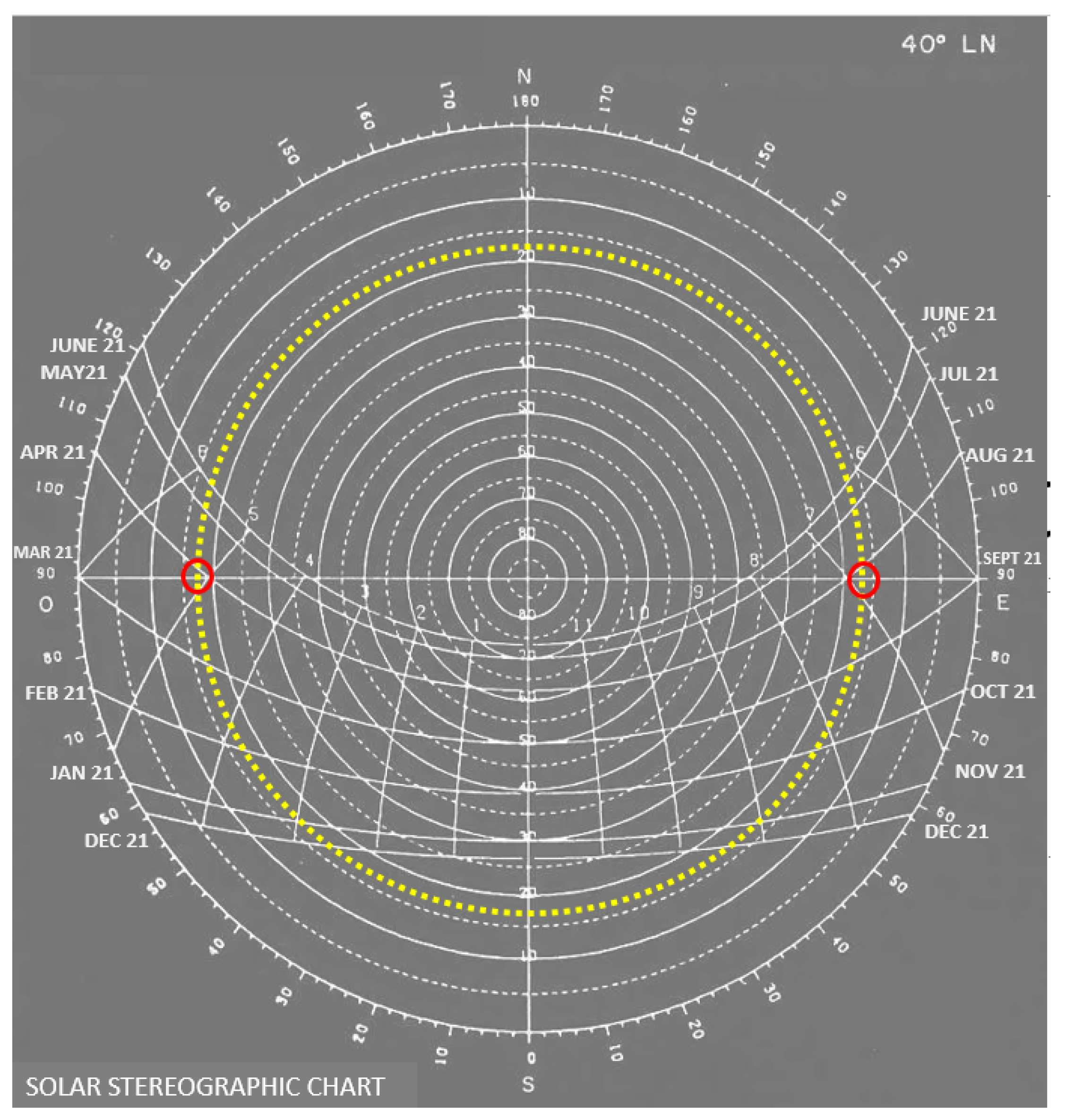
To better understand how shading evolves throughout the year, we focus on the angle of the intermediate ray within this interval. Using a spherical solar chart, we identify the two days of the year when this angle aligns with the 90° E–W position. These days represent the most critical moments in terms of shading intensity, as the rays inscribed within the limiting plane along the E–W axis are closest to their actual magnitude (real elevation angle).

Based on these reference days, additional days are selected at ten-day intervals throughout the year. These selected days are then modeled using specialized software to analyze the progression of shading over time. The two main variables examined in this analysis are the intensity of the shadows and the percentage of panel occlusion caused by the plantations.

The collected data are plotted and organized into tables to test the hypothesis that the previously identified critical day corresponds to the highest shading intensity. Additionally, the results aim to confirm that the shading caused by the plantations is minimal in both occlusion and intensity.

It is important to note that this process is not intended to quantify the annual energy losses of the solar panels. Instead, its primary objective is to assess the feasibility of integrating tree plantations of significant size within solar farms. This study aims to demonstrate their minimal impact on photovoltaic energy production while providing a clear visual and conceptual understanding of how shading from interstitial plantations occurs. Furthermore, it highlights the relevance of conducting experimental tests to validate the hypotheses of low shading impact and potential positive landscape effects associated with these plantations.

2.2. Geometry and Dynamics of the Model

The model under study consists of photovoltaic (PV) systems with solar trackers aligned along a north–south axis combined with interstitial plantations situated in the corridors between the tracker rows. These plantations are also oriented along a north–south axis to ensure uniformity in shading and spatial arrangement.

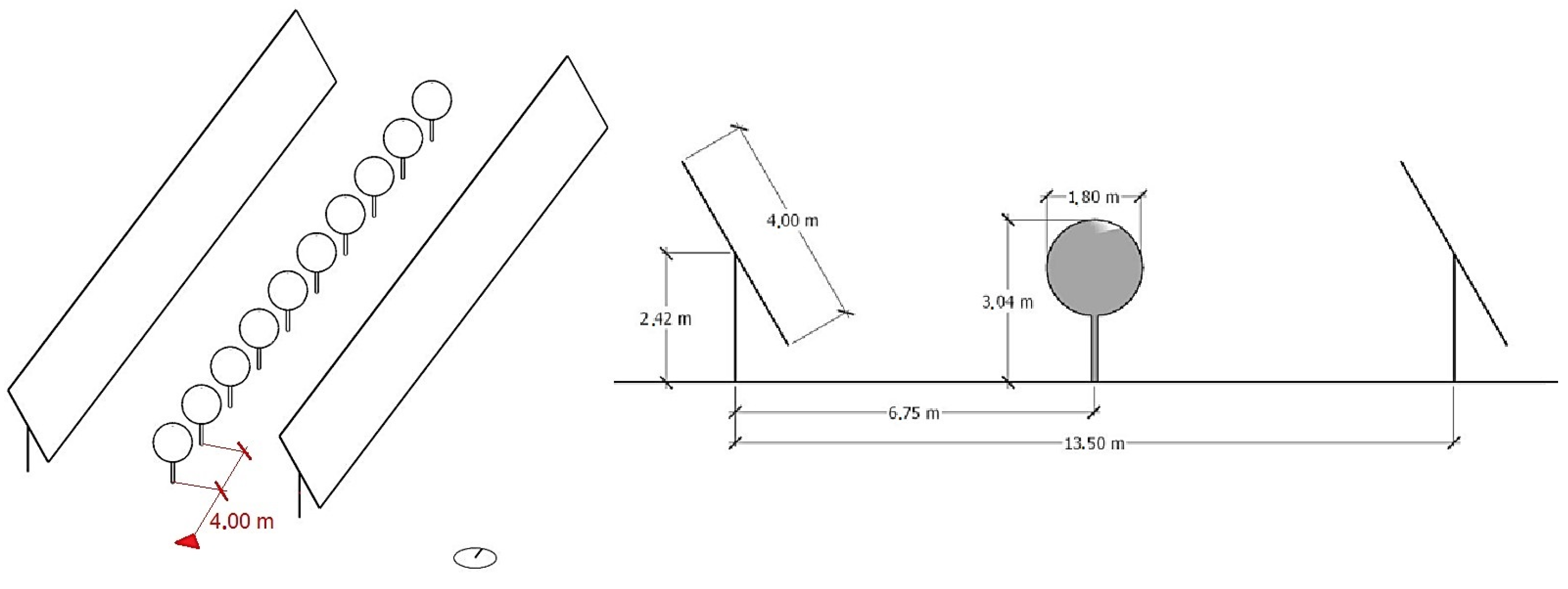
The layout is based on a real-world photovoltaic plant (PVP) with a standard geometry (Figure 1). The solar trackers are spaced 13.50 m apart, with the rotation axis of each tracker positioned at a height of 2.42 m. Each PV panel has a width of 4 m. The interstitial trees to be tested are planted centrally within the corridors, spaced 4 m apart. The trees have a crown diameter of 1.80 m and a height of 3.04 m, values determined by operational and landscape considerations. The geographic location of the PVP is at 40° N latitude.

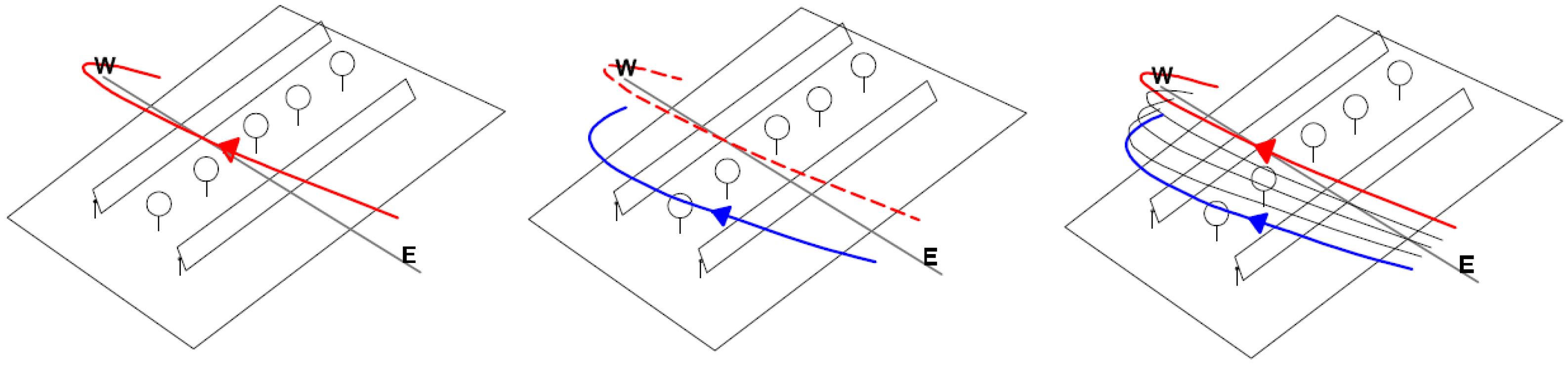
In terms of the dynamics of the model, the sun moves from east to west in a daily orbit on a plane that shifts and tilts relative to the east–west axis throughout the year (Figure 2), with a varying inclination on each day, typically represented in spherical solar charts. The sun’s position is described by two parameters: the azimuth, or angular position relative to the north–south line on a hypothetical horizontal plane, and the elevation, or the angle of incidence of the sun’s rays.

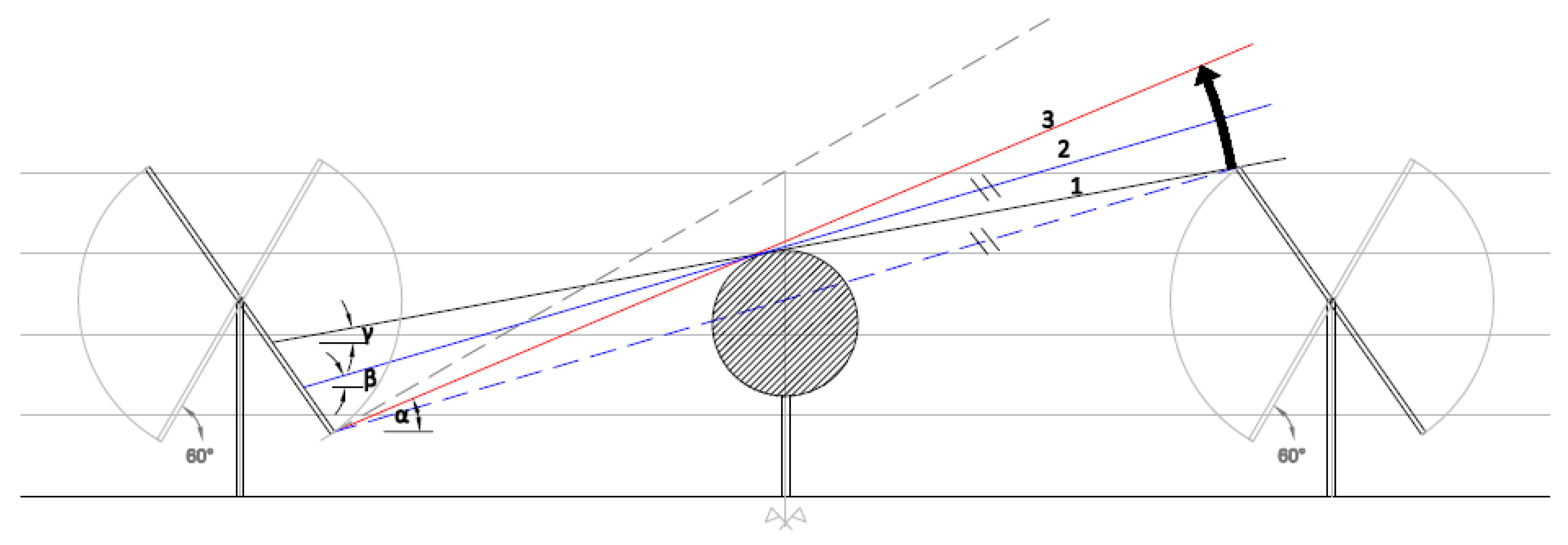
The solar trackers adjust their orientation throughout the day to optimize solar energy capture. Starting from a fixed east-facing position at 60° from the horizontal during nighttime, they begin moving as soon as the sun’s rays become perpendicular to the panels. The trackers follow the sun’s trajectory until they reach a fixed west-facing position at 60° in the afternoon (Figure 4).

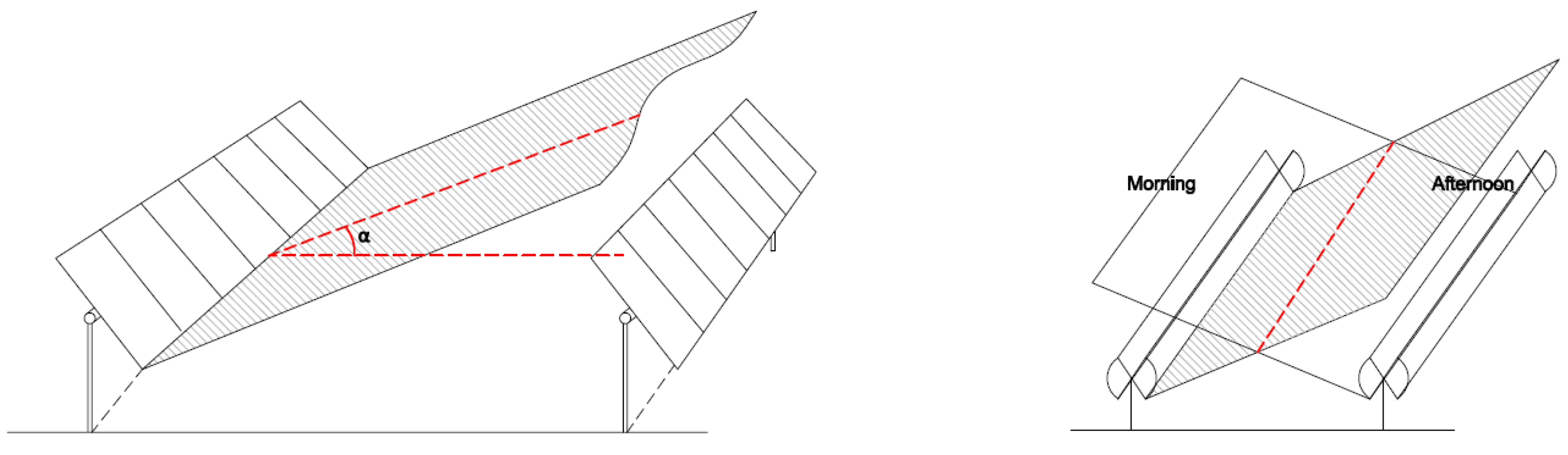
Given the interaction of the dynamic elements, which predominantly occurs in an east–west projection, the concept of a “limiting plane” is introduced for the interstitial plantations. These limiting planes set the maximum allowable height of the vegetation to prevent excessive shading. Each limiting plane is defined by a directrix, which corresponds to the lower edge of the PV panels aligned along the north–south axis.

The angle of the limiting plane, determined relative to a vertical plane perpendicular to the directrix (aligned east–west), is selected to balance shading reduction and vegetation visibility. This configuration is symmetrical, with limiting planes facing east in the morning and west in the afternoon (Figure 3).

Based on the above and to optimize the balance between vegetation height and photovoltaic efficiency, a limiting plane is defined to allow plantations to enhance the landscape without significantly impacting solar energy production. Two reference planes serve as the foundation for this approach:

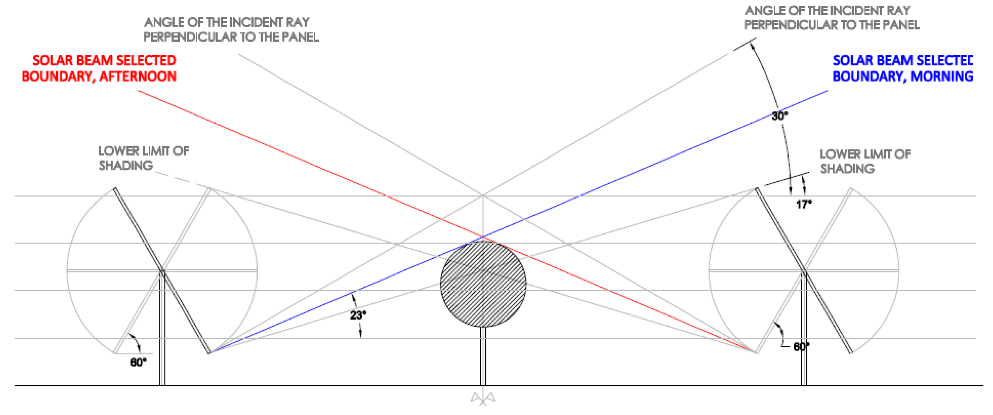
• First, based on the previous description of the model, there is a space below the plane that connects the highest vertex of the previous row of panels with the lowest vertex of the subsequent row. Trees in this space will not cast shadows on the panels. This plane (Plane A) forms an angle of 17°.
• Secondly, according to the technical guidelines, the panels start their full production when the rays are perpendicular to their resting position (60°). These rays, which form an angle of 30°, define a space below them in which trees will only cast shadows on the panels during periods just before or after they enter full production (Plane B) (Figure 4).

Selecting trees strictly below the space defined by Plane A would be overly conservative, requiring very low plantings. On the other hand, placing trees below the space defined by Plane B would be risky, as the panels would start to receive radiation before reaching full production, albeit at lower irradiance levels. Therefore, an intermediate solution is proposed by quantifying the extent to which trees interfere with solar production during the pre- and post-peak production periods. This intermediate scenario will provide valuable insights for real-world experimental applications.

In addition, two further considerations reinforce this approach:

• Low Solar Inclination: Shadows cast during early morning or late afternoon hours coincide with lower irradiance levels, reducing their impact on energy production and equipment performance [21].
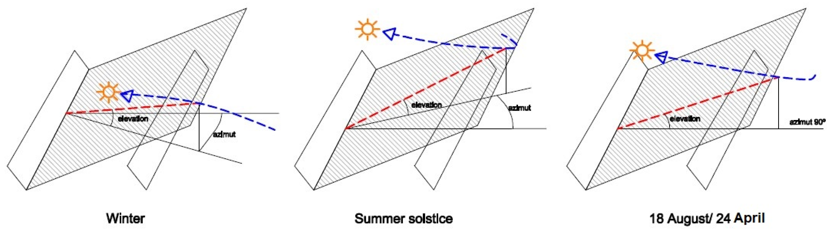
• Seasonal Variation in Solar Elevation: Once a limiting plane has been chosen, the sun’s ray coincides exactly with its real height (projected onto an east–west vertical plane) on only two days of the year (one for each solstice). On all other days, this projection shifts away from the east–west vertical plane, resulting in lower real heights. Consequently, the intensity of the shadows varies, with the worst day occurring when the central ray of the interval (the ray between the first to cast a shadow and the ray defined by the limiting plane) hits the panels in the true east in the morning (or west in the afternoon). The intensity of the shadows decreases as the year progresses towards the opposite solstice and then increases again (Figure 5).

2.3. Modeling the Intermediate Case

The shading effects of interstitial vegetation located below an intermediate plane between the two defined planes is modeled. Specifically, a 23° plane is used, positioned between Plane A (17°) and Plane B (30°).

Trees are planted along the corridor axis up to the 23° limiting plane, extending symmetrically for both the morning and afternoon scenarios (Figure 6).

As shown in the figure below (Figure 7), the trees cast shadows on the back walls during an interval that begins when the sun (ray 1) reaches angle ɣ (with respect to the east–west vertical plane), passes through ray 2 (which is geometrically parallel to angle A, 17°, see Figure 7), and ends when ray 3 reaches the chosen limiting angle α (23°).

Given the geometry of the model, the previous angles are ɣ = 11°, β = 17°, and α = 23°.

This shadow interval occurs every day of the year, but as mentioned above, the actual elevation of the sun casting these angles on the east–west vertical plane varies from day to day. The most unfavorable day is when the central ray of this interval (ray 2, with an angle of 17°) reaches the sun exactly in the true east in the morning (or in the true west in the afternoon). On other days, the interval occurs at a lower sun elevation, meaning that both the average solar irradiance and the shadows cast on the panels are weaker.

Based on this information, a general model of the phenomenon is developed by evaluating the shadows cast at three moments within the interval for each day. From these shadows, we derive two key aspects: the percentage of panel shading caused by the trees (calculated for a 4 m × 4 m panel module, based on the tree spacing) and the intensity of shading at each moment, as shown in Figure 8 below, which relates solar elevation to irradiance.

Next, we calculate an average for both aspects for each day: the average percentage of occlusion during the shadow interval and the average shading intensity of the interval.

This process is applied to four days of the year: the most unfavorable day (when the central ray of the interval is at angle β in the east–west direction) and three other days, spaced 10 days before and after on the calendar.

2.4. Selection of Representative Days and Shading Intensity Analysis

The mean angle of the interval, 17°, was selected, and a solar chart for latitude 40°N was used to identify the two days when the sun reached this altitude in an east–west orientation (i.e., the sun’s elevation relative to the vertical E–W plane, in true magnitude). The two days corresponding to this altitude and orientation were found to be 20 April and 20 August (Figure 9).

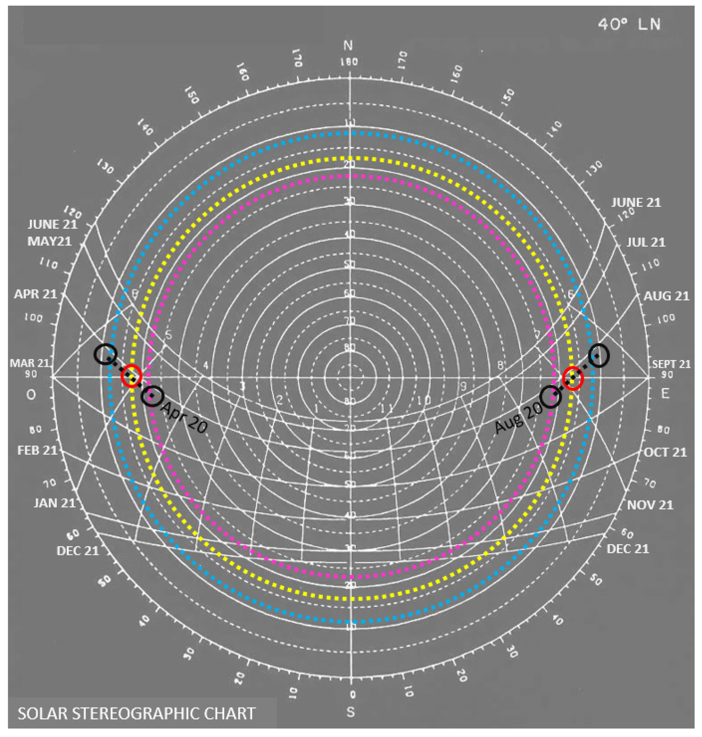
For the study, we chose 20 April as the reference day (the most critical for shading). Shading was modeled at three key moments on this day:

• Shortly after the first plant shadows appear on the panels, at a sun angle slightly above the critical angle (alpha), around 12°.
• At the central angle (beta), which is 17°.
• Just before the shadows disappear behind the previous panels, at an angle (gamma) of about 22°.

By marking these sun elevations (12°, 17°, and 22°) on the solar chart (in green and blue lines), we deduced the times when these elevations occur on 20th April (Figure 10).

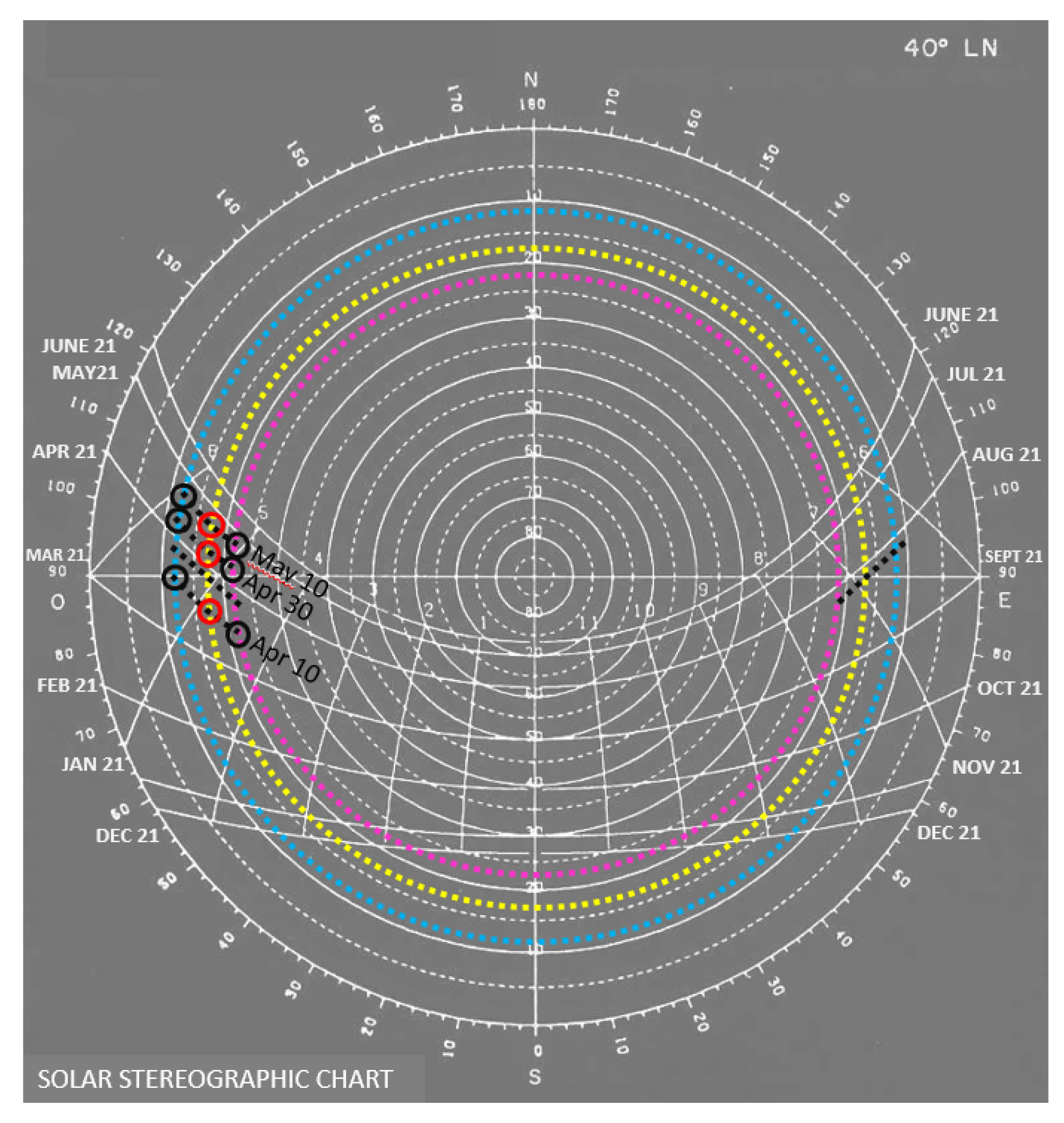
This process was repeated for three additional days spaced ten days apart: 30 April, 10 April, and, as a control, 10 May (Figure 11).

We thus have a sample of four days, each with three moments of analysis. For each of these days, the shadows were examined as follows (assuming symmetry in the afternoon):

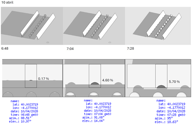
• On 10 April: 6:44 am, 7:04 am, and 7:28 am (solar times for latitude 40° N);
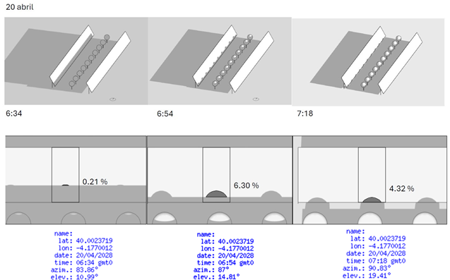
• On 20 April: 6:33 am, 6:54 am, and 7:18 am;
• On 30 April: 6:22 am, 6:42 am, and 7:09 am;
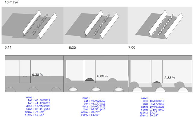
• On 10 May: 6:11 am, 6:30 am, and 7:00 am;

For each moment, the percentage of solar occlusion (shadow area) and its intensity were calculated. The percentage of occlusion was determined by modeling the scene using the SunEarth Tools software.

At these times, both the percentage of panel shading (occlusion) and shading intensity were calculated. The occlusion percentage was derived using SunEarth Tools to model the interaction of shadows with the panels, while the shading intensity was adjusted based on solar irradiance. As solar altitude decreases (e.g., early morning or late afternoon), irradiance and, consequently, shading intensity are reduced.

An irradiance model based on solar charts for 40° N latitude was used to estimate shading intensity for a typical day near the equinox (e.g., mid-March or mid-September).

Table 1. Correlation between solar time, solar altitude (solar angle), and irradiance.

Solar Time	Solar Angle	Irradiance (W/m2)
12 h PM	50°	1000
10 h PM	40°	800
8 h AM	25°	450
7 h AM	13°	300
6 h AM	5°	60

illustrates the relationship between solar time, angle, and irradiance.

We took the range of sun angles we are interested in, between 9 and 21°, and we interpolated the irradiance data from Table 1 to adjust them to this range. An irradiance of 1000 W/m² was assimilated to a shading intensity of 100% and an irradiance of 0 to a shading intensity of 0%, as shown in

Table 2. Correlation between solar angle and shading intensity.

Solar Angle	Shading Intensity
24°	0.45
23°	0.44
22°	0.43
21°	0.42
20°	0.41
19°	0.40
18°	0.38
17°	0.37
16°	0.35
15°	0.33
14°	0.32
13°	0.3
12°	0.28
11°	0.25
10°	0.22
9°	0.18

.

SunEarth Tools was used to determine the actual sun elevation for each moment analyzed, allowing both the shading intensity and the percentage of occlusion to be calculated for each event. These values were then averaged to produce a single average value for solar occlusion (area) and intensity for each day (morning and afternoon), as summarized in

Table 3. Summary of shading intensity and occlusion for each day analyzed.

Day/Time	1st Hour		2nd Hour		3rd Hour		Average
	Intensity	Shading	Intensity	Shading	Intensity	Shading	Intensity	Shading
April 10
April 20
April 30
May 10

.

By extrapolating the results at ten-day intervals, shading intensity and occlusion patterns were modeled for the remainder of the quarter.

In summary, four study days were considered, each with three episodes or configurations. This was conducted for two parameters, shading intensity and occlusion percentage. Finally, daily averages of both parameters were obtained. In total, therefore, 16 different configurations were tested (the last four being daily averages) and a total of 32 data were analyzed.

3. Results and Discussions

The results of the modeling carried out using SunEarth Tools are presented graphically for each day and hour analyzed, with a focus on the morning data. The experiment was carried out in October 2024.

3.1. Shading Analysis

Four specific dates—10 April, 20 April, 30 April, and 10 May—were selected for detailed evaluation. On each day, three time slots were analyzed to capture the actual shading effect of the vegetation on the photovoltaic (PV) modules.

Table 4. Depiction of shadows on the panels at three different times for each of the four analyzed days. The upper image shows plantings and shadows on the panels, while the lower graphs depict the solar altitude and azimuth at each moment.

April 10

April 20

April 30

May 10

illustrates these shading patterns, showing in the upper section the plant layout and its corresponding shadows on the panels, while the lower section provides the solar elevation and azimuth data at each respective moment.

From these graphical outputs, the shading intensity was calculated for each time slot. Additionally, the percentage of panel occlusion was derived by determining the ratio of the shaded area to the total panel surface area.

3.2. Daily Averages

Table 5. Summary of shading intensity and occlusion percentage (%) for each analyzed day and their daily average.

Day/Time	1st Hour		2nd Hour		3rd Hour		Average
	Intensity	Shading	Intensity	Shading	Intensity	Shading	Intensity	Shading
10 April	0.25	0.17	0.32	4.6	0.39	5.7	0.32	3.49
20 April	0.25	0.21	0.35	6.30	0.41	4.32	0.336	3.61
30 April	0.25	0.36	0.33	6.31	0.41	3.27	0.33	3.313
10 May	0.25	0.38	0.33	6.03	0.405	2.83	0.328	3.09

provides a summary of the daily averages for both shading intensity and occlusion percentage, complementing the data presented in Table 3.

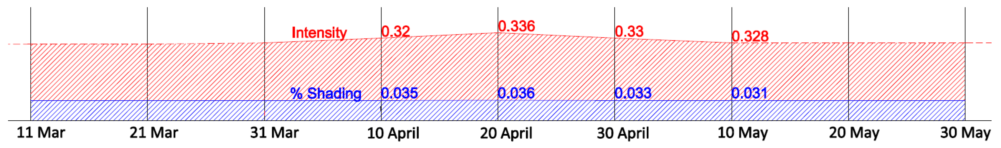
To extend these findings, the values were extrapolated at ten-day intervals for the remainder of the quarter, allowing for an estimation of shading intensity and occlusion percentage over time (Figure 12).

3.3. Interpretation of Results

The results provide important insights into the shading characteristics of the selected plantings throughout the year.

Overall, the results highlight that, under the chosen planting height—which remains below the limiting plane (the intermediate angle between negligible and perpendicular shading)—the cast shadows are minimal. Specifically, the shaded area remains below 0.04 m² on a 2 × 4 m panel, with little variability throughout the calendar year. The shading intensity ranges from 0.32 (best day) to 0.336 (worst day), indicating generally low-intensity shading. These shading episodes occur both in the morning and in the afternoon, each lasting about 44–49 min.

If we consider these results in the light of various studies on the loss of production due to shading of solar panels, for example, in Silvestre S. et al. [22], we find that the effect depends on both the intensity of the shade and the number of cells affected, as well as the arrangement of the cells, which are usually in series, and the panel technology used to avoid short circuits. In conclusion, shadows of low occlusion and low intensity can be expected in more efficient and shade-resistant panels, such as monocrystalline ones, but this needs to be verified in experimental applications of the proposal of this paper.

These findings offer valuable insights for designers of agrivoltaic systems, helping to select interstitial vegetation and optimize the light–shade interactions with photovoltaic modules while respecting the plants’ shading tolerance. Nonetheless, it is strongly recommended that these theoretical results be validated through in situ experiments to accurately gauge their impact on panel performance and efficiency.

4. Conclusions

This study demonstrates that interstitial woody plantings can be effectively integrated into north–south axis solar-tracking PV systems, providing both aesthetic and ecological benefits without incurring substantial shading penalties. By establishing a “limiting plane” at 23°, measured from the lower panel edge, the height of planted trees remains sufficient for meaningful landscape enhancement yet does not exceed thresholds that would unduly decrease solar irradiance.

The methodology, based on the above, proposes the key concept of the limiting plane to define the plantations to be installed, which will be of interest to future agrivoltaic designers. It conceptually reveals the shading process, defined by two parameters, average % occlusion and average intensity of shadows, which vary very little throughout the year. The study simply seeks to show that the intensity of the shadows reaches a maximum on two days a year and then tends to decrease. Finally, the methodology allows us to visualize graphically, for four days, what the shadows of the said plantations are like.

Computational modeling indicates that trees with a 1.2 m crown diameter, placed at 4 m intervals, cast shadows for approximately 46 to 49 min each morning and afternoon, covering on average 3.3% of the total panel surface. Peak shading intensity—close to 33.6%—occurs on a few critical days per year and then gradually diminishes to 32% over the subsequent month. Because tree crowns are composed of dispersed foliage rather than opaque surfaces, the actual impact on solar production is partially mitigated by the diffuse nature of the shadow. These findings underline how an intermediate planting height, neither too low to be visually irrelevant nor too high to interfere significantly with PV output, can aid in balancing energy generation with social and environmental considerations.

In practical terms, this approach can bolster local acceptance of PV installations by improving visual integration and potentially supporting biodiversity through pollinator habitats or agroforestry practices. The proposed geometry also offers a foundation for adaptable agrivoltaic designs, as planting species can be diversified to reflect regional conditions while maintaining the basic principles of spacing and limiting planes. Future research should verify these model predictions in real-world settings, assessing not only the impact on energy yields over different seasons but also the growth rates and health of the planted species. Moreover, potential synergies with water management, soil conservation, and carbon sequestration could expand the concept’s environmental value. In sum, interstitial woody plantings under carefully determined spatial and angular constraints offer a promising pathway toward more sustainable, multifunctional photovoltaic landscapes.