A Ray-Tracing-Based Irradiance Model for Agrivoltaic Greenhouses: Development and Application

Abstract

A key challenge in designing agrivoltaic systems is avoiding or minimizing the negative impact of photovoltaic-induced shading on crops. This study introduces a novel ray-tracing-based irradiance model for evaluating the irradiance distribution inside agrivoltaic greenhouses taking into account the transmission characteristics of the greenhouse’s cover material. Simulations are based on satellite-derived irradiance data and are performed with high spatial and temporal resolution. The model is tested by reproducing the agrivoltaic greenhouse experiment of a previous study and comparing the simulated irradiance to the experimentally measured data. The coordinates of the sensor positions in the presented application are optimized based on one day of raw data of minutely measured irradiance from the experimental study. These coordinates are then used to perform simulations over an extended timeframe of several months to take into account the seasonal changes throughout a crop cycle. The average deviation between the simulations and the experimental measurements in terms of radiation reduction is determined as 2.88 percentage points for the entire crop cycle.

1. Introduction

By launching the European Green Deal in 2020, the European Commission aims to make Europe the first carbon-neutral continent by 2050. This includes the 2030 Climate Target Plan, which seeks to reduce greenhouse gases by 55% by 2030 [1]. Increasing photovoltaic (PV) energy production is a suitable approach, since large-scale PV systems have proven to be green, cheap, and reliable energy sources. In many countries, the targets of the Paris Agreement to increase the share of renewable energies for combating climate change have triggered direct land use changes in order to meet the objectives of different European Union (EU) programs. Ground-mounted PV-systems have been installed on arable land formerly used for food production, and high-quality soils have been taken out of agricultural production [2].

However, renewable energy does not threaten agricultural production; indeed, they can coexist in harmony. Agrivoltaics (APVs), a form of solar sharing or dual land use, is a concept that combines agriculture and photovoltaic (PV) systems, allowing for the simultaneous use of land for crop cultivation and solar energy production. Recent studies have already reported the positive effects of the shade from PV panels on plant microclimate and growth [3,4].

The Joint Research Center estimates that 5.2% of the land in the EU is ideally suited for accelerated renewable deployment, excluding natural protected areas and high-value agricultural land [5]. Yet, the European Environmental Bureau’s latest report finds that only 2.2% of the EU’s land area would be needed to accommodate sufficient renewable energy sources to entirely replace fossil fuel and nuclear generation [6]. Using APV alone could surpass the EU photovoltaic 2030 goals [5].

In southern Spain, especially in the region of Almería, an area of over 30,000 ha is occupied by greenhouses (GHs). These GHs use plastic covers to manage light and heat, crucial for year-round crop cultivation [7]. However, the excessive sunlight in summer requires farmers to reduce light transmission, often achieved by applying white chalk paint [8]. In addition, there are other techniques to reduce light transmission and manage the GH microclimate, such as the use of shading nets (applied internally or externally) [9], thermal screens [10], or even wavelength-selective plastic films, that block out a fraction of the infrared spectrum [11,12]. APV concepts can actively support this light management by the growers, and sunlight could additionally be used to produce energy. Hence, the energy efficiency in agriculture could be improved, which directly translates into a higher profitability for farmers. According to Dupraz et al. [13], APV GHs can increase the productivity of crops by up to 73% in crops benefiting from low-light conditions. They can also reduce the dependence on energy, the prices of which are rising, through PV production and the self-consumption of electricity and heat [14]. Hanrieder et al. showed that it is possible to provide up to 44% shading for plastic GHs without reducing crop yields [15].

Designing and optimizing APV GHs involves several challenges. First of all, all APV installations must comply with legal requirements. Following the definition of APVs the main priority remains continuous agricultural production [16]. As photosynthesis is the key process in producing biomass, sunlight is one of the most important environmental factors influencing plant growth and eventually the yield in GHs [17]. In addition to radiation, the directional irradiance distribution throughout the canopy also plays an important role [18]. Several studies showed that plants more efficiently use diffuse light, which leads to a more homogeneous light profile in the plant canopy, than direct light [19,20,21]. However, in open-field agrivoltaic systems, the radiation transmitted through PV panels can significantly change its spectral composition with important effects on plant growth and development [22].

Cossu et al. summarized results of numerical simulations as well as experimental results of GHs in Europe with PV cover ratios of 25% to 100% [17]. The simulations showed a yearly global radiation decrease by 0.8% for east–west-oriented and 0.6% for north–south-oriented GHs for each additional 1% PV cover ratio. The results also indicated that a north–south orientation and the arrangement of PV modules following a checkerboard pattern improve light distribution uniformity. The experimental studies of Ezzaeri et al. [23] and Aroca-Delgado et al. [24,25] investigated the effect of up to a 10% PV cover ratio on tomato crops, with PV panels mounted in a checkerboard pattern on typical Mediterranean GHs. Both studies showed that, in this range of cover ratio, no significant negative effect on total and marketable production was observed.

Pilot sites across Europe show that the design of APV solutions always has to be adapted to location-specific climatic conditions [26]. So far, experimental studies have been limited to specific GH typologies and conditions, where the location, orientation, geometry, and materials of GHs vary substantially from one to another, therefore leading to different findings. Also, due to the high cost of irradiance sensors, experimental studies have been limited to measurements of distinct, localized irradiance measurement points and did not consider spatial irradiance distribution or light homogeneity throughout the GH.

Therefore, simulation models to estimate radiation distribution and uniformity are needed. Different modeling approaches have been developed so far. Kempkes et al. employed ray tracing calculations to determine novel roof concepts to increase light transmission in a Venlo-type GH located in the Netherlands [27]. Laue et al. used ray tracing algorithms to investigate the effect of bifacial PV modules on the energy production and radiation levels inside a glass GH located in Norway [28]. Cossu et al. developed a model to simulate the temporal irradiance distribution inside GHs [17,29]. Furthermore, additional models that evaluate the reduction in the total solar radiation in APV GHs have been developed [30,31,32,33]. However, none of them address the impact of the PV modules’ layout on the spatial radiation distribution. Torrente et al. [34] developed a simulation tool to calculate the irradiance uniformity inside a Venlo GH by applying a decomposition model, based on the method developed by Pulido-Mancebo et al. [35]. The method was originally used to simulate the global horizontal radiation distribution in open-field APV systems.

For photosynthesis, plants capture a fraction of the total radiation spectrum, the so-called photosynthetic active radiation (PAR) spectrum, which includes wavelengths from 400 nm to 700 nm. There are different modeling approaches that focus on modeling the PAR for APV installations. Ma Lu et al. recently proposed a re-parameterization of seven different decomposition model splitting global horizontal irradiance (GHI) into direct and diffuse PAR fractions to model the PAR radiation distribution in open-field APV installations in Sweden [36]. Regarding GHs, as the optical properties of the GH cover materials directly influence the light transmission and therefore the distribution of diffuse and direct PAR radiation perceived by the crops, the sole use of decomposition models is not directly applicable. Another practical and efficient method for estimating the PAR is the use of linear regression models. Different linear regression models have been developed for various regions to account for local climatic conditions. For example, Zainali et al. [37] recently presented a linear regression model specific to Sweden. A different approach is the estimation of hte minimum light requirements for site-dependent types of GH cultivation, as described by Schallenberg-Rodriguez et al. [38].

In this work, we present a comprehensive model for accurately simulating the spatial and temporal irradiance distributions inside APV GHs by using a ray-tracing-based approach. Temporal resolution as well as spatial resolution can be defined depending on the application. Simulations can be performed with a high temporal resolution, with time steps below one hour, hence giving a clear picture of irradiance distribution on a fine time scale. Furthermore, the 3D ray tracing approach allows the user to define a high spatial resolution and examine any point of interest inside the virtual GH. A detailed study of the correct representation of GH cover materials in the simulation was performed, incorporating the effect of diffuse light transmission. The integration of satellite-derived irradiance data enables the evaluation of different locations and timeframes specified by the user. Overall, the model allows the implementation of digital twins of real-scale GHs with a PV pattern in a layout specified by the user, giving a clear picture of the effects of partial shading on GH plants.

The application of ray tracing algorithms to plastic GHs and the accompanying high level of detail is the novelty of this model in comparison to other simulation tools. The models developed by Cossu et al. [17] and Torrente et al. [34] calculate temporally averaged light distribution maps for APV GHs. The approach of Cossu et al. estimates the annual average values of the global solar radiation within GHs equipped with PV modules [17]. The impact of different PV cover ratios, orientations, and structural parameters on light uniformity and availability is evaluated over the course of a year, and, therefore, their model cannot highlight short-term fluctuations due to local weather conditions or diurnal variations [17]. The approach of Torrente et al. [34] provides a vector-based geometric representation of the GH and PV panels. To determine the solar radiation entering a GH, any given point inside the GH is assessed if it is shaded by PV panels or exposed to direct sunlight, depending on the solar position. Irradiance maps for the GH ground are then estimated based on solar irradiance for representative days in each month taken from a typical meteorological year (TMY). By integrating these values over time, the model estimates both monthly and annual radiation levels for different points inside a GH and provides averaged irradiation maps for the GH’s ground.

The presented model, on the other hand, includes a very detailed representation of the GH structure and the cover materials. Simulations are based on satellite-derived irradiance data instead of averaged annual irradiation values or TMY files. In comparison to other models, the presented approach highlights the influence of local environmental conditions, different sun positions, as well as the shading caused by the GH structure itself. The limitations of the presented model include the simplified approach for modeling GH plastics and the angular-dependent light transmission, the inhomogeneous soiling of GHs and material degradation, as well as the suitability of the model for performing long-term analysis. All these limitations of the model are discussed alongside with the methodology. As ray tracing simulations can be computationally extensive, this paper also includes a section about computational resources and the applicability of the model.

This paper is structured as follows: Section 2 includes the technical description of the model and describes the overall model workflow. The model was directly applied to a Venlo APV GH from a previous experimental study. Section 3 presents the validation of the presented model. Section 4 focuses on the computational effort related to ray tracing simulations. Section 5 interprets the results and compares them with previous studies. Section 6 discusses the outcomes of this study and gives an outlook on further developments.

2. Materials and Methods

The objective of the model is to assess how PV modules on GHs affect the irradiance distribution inside the GH with high spatial and temporal resolution. Therefore, a ray-tracing-based approach was chosen, utilizing Radiance software, version 5.4 [39]. In this work, we focused on light transmission through GH cover materials, the adaptability of PV arrangement patterns, and the simulation of GHI distributions inside APV GHs. For additional information on the PAR derived from the simulations, the model could be coupled, e.g., to a linear regression model to change from GHI to PAR, such as to the methods developed by Zainali et al. [37] or Vindel et al. [40].

The design and orientation of the GH, the location coordinates, and the arrangement of the PV modules are defined first. This geometrical scene is then combined with input solar radiation data. Ray tracing simulations are performed with a temporal and spatial resolution defined by the user. To test the model, we present the implementation of an experimental APV GH, which was evaluated in a previous study by López-Díaz et al. [41]. The experiment was conducted from 17 September 2014 to 14 May 2015. The simulations presented in this manuscript were conducted in 2024 and are covering the time period of the experiment.

2.1. Model Inputs

The model has three main inputs: geometrical details, material properties, and irradiance data.

2.1.1. Geometrical Details

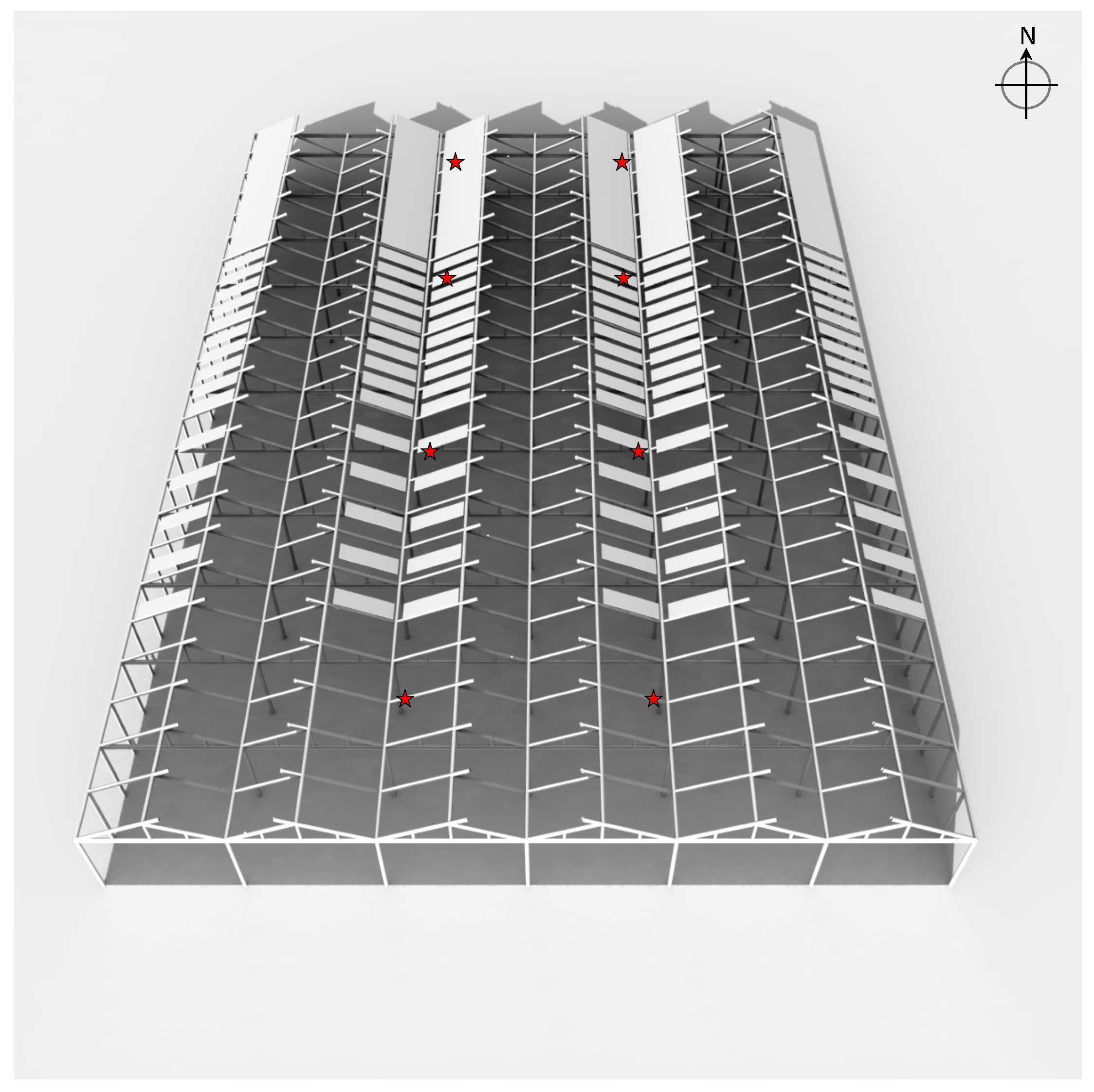
The geometrical details of the GH structure and its materials have to be defined, so that a 3D representation of the GH can be generated first. Depending on the available roof area and the desired roof cover ratio, the model allows the user to distribute PV modules on the GH roof. Individual PV modules are defined as rectangles with user-defined dimensions. In this study, PV modules were modeled with a fully opaque material, but semi-transparent modules can also be implemented in the future. The GH dimensions and the PV module configuration are adapted to the case study. In the developed model, the user can specify the PV module arrangement pattern, e.g., checkerboard or linear placement and the coverage ratio. Then, the model automatically computes the number of PV modules and the gaps considering both the roof and module dimensions.

The experiment presented by López-Díaz et al. took place from from 17 September 2014 to 14 May 2015 in a Venlo-type GH covering an area of 2145 ${\mathrm{m}}^2$ ($57.5$ $\mathrm{m}$ long in north–south-direction, and $42.0$ $\mathrm{m}$ width in east–west-direction) at the Tecnova experimental center in the province of Almería, southern Spain (36°53′ N, 2°22′ W, 185 $\mathrm{m}$ above sea level) [41]. The experimental design consisted of three shaded zones (15%, 30%, and 50% roof area covered) and a 0% control zone without any shading. Based on the information given by López-Díaz et al. in [41], a virtual copy of the experimental test GH was implemented in the simulation framework. Each zone was equipped with two radiation sensors. Figure 1 presents the final GH implementation and the estimated sensor positions.

2.1.2. Material Properties

In the current version of Radiance, implementing realistic GH plastic materials is a challenging task. In general, transmissive materials can be implemented using the Radiance material category $trans$. A more detailed explanation of the parameters required for that category is included in Appendix A.1. In most cases, it is not possible to have accurate information on all these parameters. For this reason, this model uses a more simplistic approach to characterize the optical properties of the material. This technique only requires two inputs to describe the transmission properties of the material: $T_{diff}$ and $T_{spec}$. Both parameters can range between 0 and 1. $T_{diff}$ refers to the diffuse transmission of the material, while $T_{spec}$ describes the specular transmission.

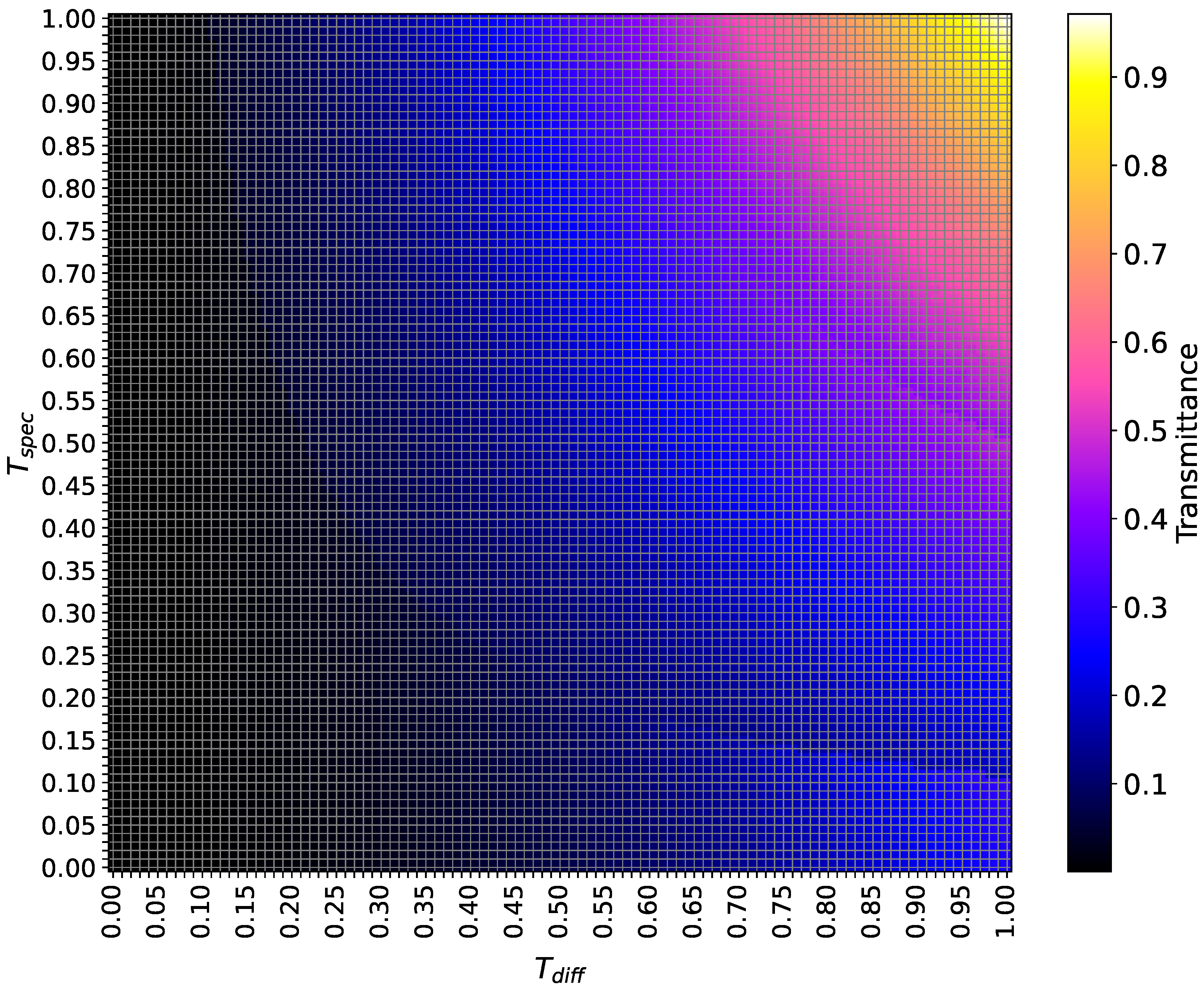
Usually, the only available information when purchasing plastic sheets for GHs is the transmittance value, without separation into direct and diffuse fractions. In order to be able to relate the overall transmittance of a material to a combination of $T_{diff}$ and $T_{spec}$ in Radiance, a sensitivity analysis was performed.

A test environment for $trans$ materials was set up with a rectangular surface of the material at a specific height. A light source was simulated above the material, sending out rays with a constant intensity. These rays passed through the material, and the transmitted irradiance underneath it was then analyzed. For the analysis, the first five parameters of the material definition were kept constant while using different pair-wise combinations of $T_{diff}$ and $T_{spec}$. $T_{diff}$ and $T_{spec}$ were varied from 0 to 1 in steps of 0.01. The overall transmittance, i.e., the ratio of transmitted irradiance to incident irradiance, was then determined for all the tested combinations. Figure 2 depicts the results of the sensitivity analysis.

The plot shows the distinct structures and color patterns for the different combinations of $T_{spec}$ and $T_{diff}$. For $T_{diff}$ values below 0.30, the tested materials all had overall transmittance values below 0.10 independent of the $T_{spec}$ value. The overall transmittance started to increase with the simultaneous increases in $T_{diff}$ and $T_{spec}$. Transmittance values of approximately 80% to 89% are described by the yellow area in the upper right corner in Figure 2. For $T_{diff}$ (as well as $T_{spec}$), values between 0.80 and 1.00 are suitable, still depending on the choice of $T_{diff}$ accordingly (or $T_{spec}$). For a given transmittance of a known GH cover material, the possible combinations of values for $T_{diff}$ and $T_{spec}$ move along a curve in Figure 2.

The presented methodology is a simplified approach for simulating light transmission through GH cover materials with Radiance. In the simulation, plastic cover materials are modeled as uniform surfaces with constant material properties and uniform transmission properties. The time-dependent changes in material properties and transmission values are not accounted for but can be the subject of future studies. In the real world, low-density polyethylene (LDPE) films are widely used as GH covering materials in the Mediterranean region, primarily due to their affordability, remarkable mechanical attributes, and exceptional resistance to chemicals [42]. These plastic films are often multi-layered with a UV-protection film toward the outside and agrochemical-resistant films toward the inside of the GH [41]. The materials have been developed to maximize the fraction of diffuse light inside GHs, with a transmission dependent on the angle of the incident light  [43,44]. In Radiance, the $trans$ material is designed to model transmissive surfaces with diffuse transmission [39]. $trans$ materials do not inherently account for complex, angle-dependent transmission properties. While more advanced material definitions, such as $transdata$ material, can incorporate angular-dependent transmittance [39], their implementation would require detailed experimental measurements of the incident-angle-dependent transmission profile of the GH cover materials, which are often not available.

In the simulation, the virtual GH consists of a large number of surface points, each with a different angle of incidence. Each of these incident points contributes to the diffuse light profile inside the GH. Furthermore, Figure 2 shows that in order to achieve a realistic overall transmittance of the material, high values of $T_{diff}$, which causes the diffusing effect, are needed. Hence, the approach of using two parameters ($T_{diff}$ and $T_{spec}$) to describe light transmission in the simulation is considered sufficient. Nevertheless, the simplification can still pose limitations to the application of the presented model. If diffuse light transmission is not 100% correctly modeled and the direct contribution of the incident rays is overly pronounced, these could lead to a geometrical mismatch in the irradiation maps. However, such an effect was not observed in the presented application of the model or in the results presented in Section 3.

The plastic cover of the experimental GH in López-Díaz et al. had a thickness of 200 $\mathrm{\mu }$$\mathrm{m}$ and a transmission of 84% [41]. Based on Figure 2, the parameter range for suitable $T_{diff}$ and $T_{spec}$ combinations was determined to match the overall target transmission of 84%. Testing different parameter combinations yielded in $T_{diff}=0.892$ and $T_{spec}=0.796$. The final material definition is given in

Table A1. Parameter definition of the $trans$ material to match the description of the greenhouse (GH) plastic used by López-Díaz et al. [41].

$\mathit{Red}$	$\mathit{Green}$	$\mathit{Blue}$	$\mathit{Specularity}$	$\mathit{Roughness}$	${\mathit{T}}_{\mathit{diff}}$	${\mathit{T}}_{\mathit{spec}}$
0.938	0.938	0.938	0.010	0.000	0.892	0.796

.

2.1.3. Satellite-Derived Irradiance Data

Irradiance conditions (i.e., GHI, diffuse horizontal irradiance (DHI), direct normal irradiance (DNI)) and the solar position must be specified to generate a description of the light sources in the simulation. In the presented model, satellite-based irradiance data, provided by the Copernicus Atmosphere Monitoring Service (CAMS), are used to generate outside irradiance conditions of the GH and simulate the inside irradiance for each investigated timestamp. CAMS products are quarterly benchmarked against a variety of ground stations to monitor their consistency. One of the regular benchmarking sites is CIEMAT’s Plataforma Solar de Almería, located approximately 30 $\mathrm{k}$$\mathrm{m}$ from the location of the GH of López-Díaz et al. at the Tecnova research facilities. A standard uncertainty of 2% for GHI measurements was estimated based on the RMSE, as described by Forstinger et al. [45].

The use of satellite-based irradiance data makes the model flexible in simulating different locations and time periods. With the latest CAMS product (version 4.0 of the CAMS radiation service), time series of GHI, DHI, and DNI are available from 2004 to the day before yesterday [46,47]. Additionally, the temporal resolution of the simulations can be adjusted based on the user’s needs. For localized, detailed simulations, a high temporal resolution, such as 15 min, is recommended. For a more general analysis of the irradiance distribution, a lower temporal resolution with 1 h intervals may be sufficient. The choice of temporal and spatial resolution and the related computational efficiency is further discussed in Section 4. In the model, the sun position is calculated using a PVlib (V0.9.4) Python routine [48,49] and combined with the CAMS irradiance data in the Radiance sky file.

The presented simulations were performed with a 15 min resolution. The input CAMS irradiance data represent the mean values for the respective 15 min. For each 15 min interval, the sun’s position was modeled at the middle of this interval. For example, for the period from 12:00:00 to 12:15:00, the sun’s position was modeled at 12:07:30.

2.2. Ray Tracing Analysis

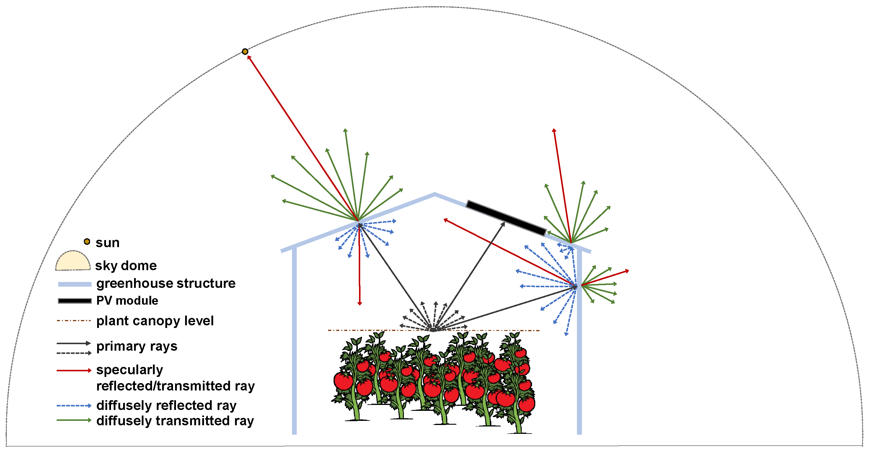
The presented model evaluates irradiance at the x-, y-, and z-coordinates provided by the user. The number of coordinates, or pixels, defines the spatial resolution of the irradiance scan. Figure 3 illustrates the ray tracing procedure for the presented model.

When a ray strikes a PV module, it is absorbed. Rays are reflected both specularly and diffusely when they hit parts of the GH support structure, with diffuse reflections generating new primary rays. When interacting with the transmissive GH cover material, rays can also be transmitted both specularly and diffusely.

For the application of the model to the APV GH of López-Díaz et al., the positions of the radiation sensors in the experiment had to be transferred to the simulation. First, the x- and y-coordinates of all eight radiation sensors in the experiment were estimated based on the description in [41]. We assumed that there might be a geometrical mismatch between the estimated coordinates and the respective coordinates in the simulation, since the virtual GH was designed based on the general description given in [41]. To account for this uncertainty, a search window of $2 \mathrm{m}\times 2 \mathrm{m}$ with a resolution of $\Delta x=\Delta y=0.05 \mathrm{m}$ was applied around the primary estimated coordinates of each sensor. For each search window, containing ${41}^2=1681$ coordinate sets, ray tracing simulations were performed with a 15 min temporal resolution for 23 January 2015. This day was chosen for the detailed optimization of sensor position because it was the only day for which raw data from all eight radiation sensors were still available.

For each sensor and for each of the 1681 simulated points, the normalized root mean square error (nRMSE) was calculated, according to Equation (1).

$$\mathrm{nRMSE}={\displaystyle \frac{\mathrm{RMSE}}{\overline{y}}}={\displaystyle \frac{\sqrt{\frac{1}{n}{\sum }_{i=1}^n{(y_i-{\widehat{y}}_i)}^2}}{\overline{y}}}$$

(1)

The parameters have the following meanings:

• n: number of observations;
• $y_i$: experimentally measured value at the i-th instance;
• ${\widehat{y}}_i$: Simulated value at the i-th instance;
• $\overline{y}$: mean of the experimentally measured values, calculated as $\overline{y}={\displaystyle \frac{1}{n}}{\sum }_{i=1}^n{y}_i$.

The sensor coordinates in the simulation that best matched the experimentally measured values were identified by minimizing the nRMSE for the specific day. Figure 4 presents the distribution of the nRMSE values for the west sensor in the 0% control zone.

The set of x- and y-coordinates, i.e., the best pixel, can be identified clearly and yields an nRMSE value of 0.1. The pixel of the initial guess of the sensor position has an nRMSE value of 0.22. The nRMSE distribution of the presented sensor shows that values can range between 0.1 and 0.5 within a distance of less than $1.00$ $\mathrm{m}$.

Using this approach, the coordinates for all eight virtual sensors were optimized and applied to simulate the entire crop cycle of the experiment, i.e., from 17 September 2014 to 14 May 2015. During the GH experiment of López-Díaz et al. in 2014/2015, the height of the radiation sensors was continuously adjusted to match the canopy level of the growing tomato crops. Consequently, the height of the irradiance scan in the simulations was gradually increased from 1 $\mathrm{m}$, reaching a final value of $2.5$ $\mathrm{m}$ at the end of the study period.

3. Validation

3.1. Simulation of One Day

As described in Section 2.2, the optimization of sensor position in the simulation was performed based on the data from one specific day, i.e., 23 January 2015. As this was the only day that experimental raw data were still available, the comparison of the time-series data of the irradiance simulation and experimentally measured values can only be presented for that day. To quantify the deviation between the simulation and experimentally measured data, the nRMSE, which was already defined in the process of coordinate optimization, and the irradiation error were calculated. The irradiation error was calculated according to Equation (2), with the same parameter descriptions as previously mentioned.

$$\mathrm{Irradiation}\mathrm{Error}(\%)={\displaystyle \frac{{\sum }_{i=1}^n\left({\widehat{y}}_i-y_i\right)}{{\sum }_{i=1}^n{y}_i}}\times 100$$

(2)

Figure 5 shows the simulated irradiance in comparison to the experimentally measured data on that day for all eight sensors.

The simulated irradiance curves align with the experimentally measured values, showing that the model is capable of simulating the measured irradiance conditions inside the GH on the presented day. Focusing on the two sensors in the 0% shading zone, the experimentally measured values display fluctuations even though there is no artificial shading from PV modules in this area. This suggests that the differences in irradiance measurements are influenced by localized shading from the structural elements of the GH that obstruct the sensors’ field of view.

Furthermore, the experimentally measured data show short-term fluctuations at a minute level for all sensors despite clear-sky conditions outside, as indicated by the GHI curve. The possible explanations for these fluctuations are that the roof is not homogeneously soiled, and thus changes in the irradiation measurement at the same location in the GH are possible due to slightly different sun positions. Other potential factors are sensor soiling due to the GH environment and general inhomogeneities of the plastic cover, e.g., small holes in the plastic or localized abrasion of the plastic cover due to the influences of wind, sun, rain, and other external factors.

The simulation generally aligns well with the overall shape of the curves of the experimentally measured data for all sensors on the presented day. Additionally, the model can simulate changes in the irradiance distribution throughout the day at a sub-hourly temporal resolution. This confirms an accurate representation of the GH structure based on the general description in [41] and justifies the optimization of the sensor coordinates.

For the presented day, the nRMSE values range from 0.08 to 0.13, and the irradiation error remains below 5% for all sensors. However, for other days, the bias and nRMSE values might be higher, as the sensor positions were fine-tuned based on the same day’s data.

Notably, the simulations of the two sensors in the 50% shading zone show the highest agreement with the experimental measurements and the lowest irradiation error values, despite the overall low absolute irradiance levels. On the west side of the 50% shading zone, irradiance values remain below 100 $\mathrm{W}$/$\mathrm{m}$⁻² during the first half of the day. In contrast, for the sensor on the east side, this occurs during the second half of the day. The model replicates these patterns, highlighting the advantage of high-resolution irradiance simulations.

3.2. Radiation Reduction for an Extended Time Period

The radiation reduction was evaluated based on the simulations of the whole crop cycle, i.e., from 17 September 2014 to 14 May 2015, at the previously chosen grid points (averaged for the two sensors per zone). Figure 6 shows the overall reduction in radiation for the three shading zones with respect to the control zone.

The simulation produces radiation reduction values consistent with the experimentally measured data. This means that the model is capable of taking into account changing outside climatic conditions and solar zenith over a prolonged timeframe of several months. For both the simulation and experimentally measured data, the presented radiation reduction values are generally higher than the roof cover ratio. López-Díaz et al. reported a radiation reduction of 28.8% for 15% shading, 46.6% for 30% shading, and 66.3% for 50% shading. In comparison, the presented simulation leads to values of 26.6%, 44.2%, and 62.4% for the respective shading zones, which is on average 2.88 percentage points lower than the experimentally measured data.

In Figure 5, the east radiation sensor of the 0% shading zone recorded higher irradiance values compared to the west sensor in the same zone. Additionally, the experimentally measured irradiance exceeds the outside GHI taken from the CAMS database on the presented day several times. Hence, if there were systematically higher irradiance readings from one of the sensors in the control zone in the experiment, this could have resulted in overall lower values in the analysis of the simulations.

Furthermore, deviations can also be caused by geometric mismatches, such as discrepancies in the overall GH structure and small misalignments in sensor positioning relative to the GH structure. Additionally, in the real world, the material properties of a GH cover can change over time due to progressive degradation, which causes a change in their visible appearance, as well as in their chemical structure, and consequently affects their physical and mechanical properties [50]. Degradation is mostly caused by exposure to UV radiation [51,52]. Other factors that also intervene, albeit to a lesser extent, are air temperature and humidity, possible mechanical stress (especially caused by wind), contact with agrochemicals, and possible internal stress related to the installation phase [50,53]. As the degradation of the material is an important aspect, it should be considered in future research and applications of the model. In addition, the model uses a simplified approach to model the light transmission through the GH cover, and the angular dependence of the incident light might lead to deviations in the long-term analysis. Furthermore, the radiation sensors in the experiment might have been soiled or affected by the local environmental conditions inside the GH or even shading by the crops, which could have also caused deviations in the presented comparison.

4. Analysis of Computational Resources

Balancing computational efficiency and the desired accuracy is crucial for ensuring both the reliability and practical applicability of the presented model. Accuracy is referred to as the spatial resolution in the x- and y-directions, relating to the number of pixels chosen for the ray tracing scan.

The presented simulations were run on a high-performance computer running Ubuntu 18.04 LTS, equipped with dual 64-bit CPUs clocked at $2.6$ $\mathrm{G}$$\mathrm{Hz}$ and 512 GB of DDR4 memory operating at 3200 MT/s.

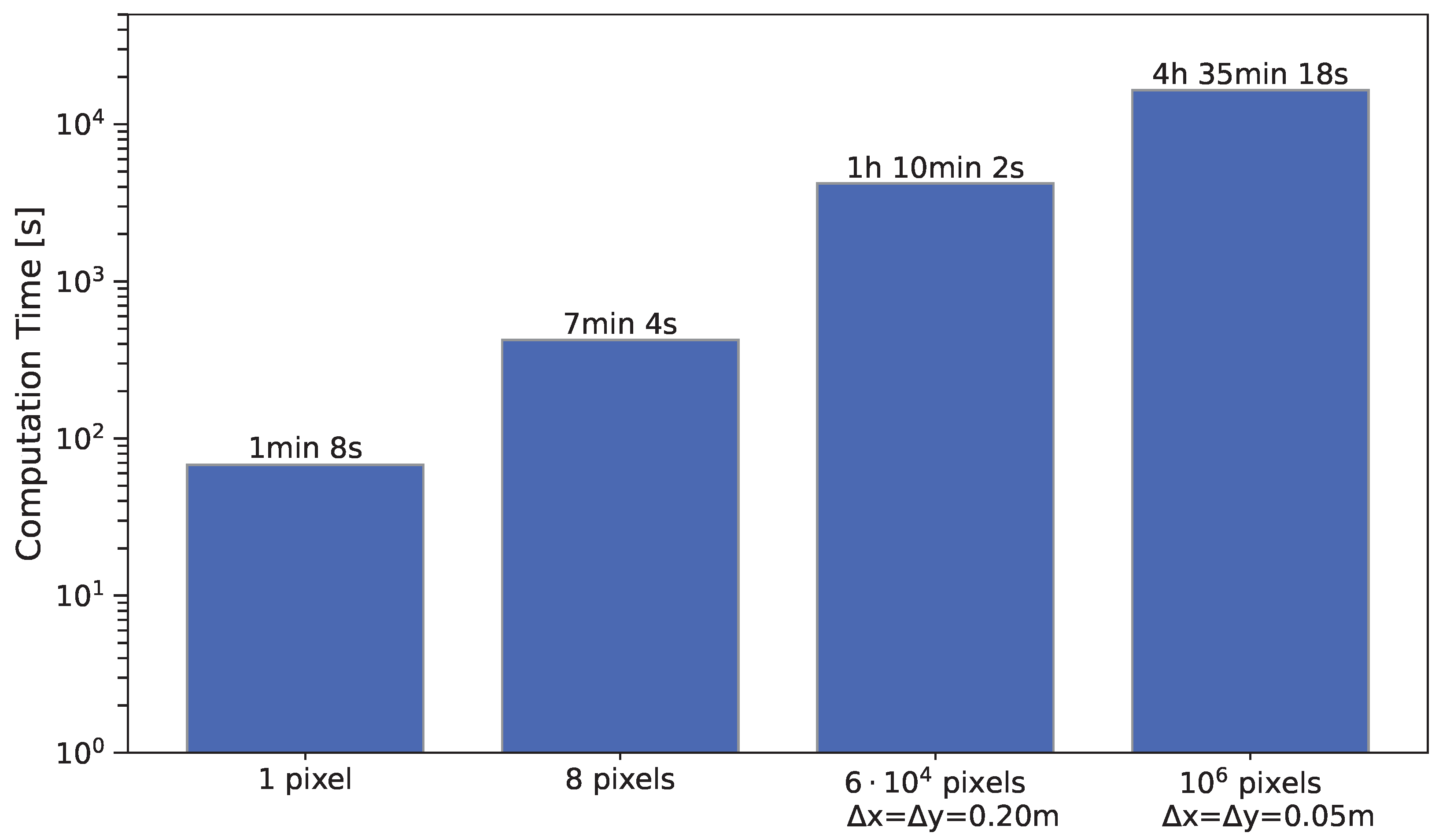
Figure 7 relates the number of pixels and spatial accuracy to the computation time for the presented application of the model to the APV experiment in López-Díaz et al.

Using a theoretical resolution of $\Delta x=\Delta y=0.05 \mathrm{m}$ for the virtual GH requires approximately ${10}^6$ virtual sensors. Under these conditions, simulating 23 January 2015 at 12:00 would take 4 h 35 min 18 s. Reducing the resolution to $\Delta x=\Delta y=0.20 \mathrm{m}$ lowers the computation time to 1 h 10 min 2 s. When simulating only the eight specified sensor positions, the runtime is 7 min 4 s. With the same configuration, the simulation of one single pixel takes 1 min and 8 s.

In Figure 5, each sensor has 37 simulated data points (from 8:15 to 17:30 in 15 min intervals), resulting in a total of 296 simulations for that day. By running 30 timestamps in parallel, the entire day’s simulations for all sensors are completed in approximately one hour, assuming each timestamp requires the same computation time. Extending this approach to cover the full crop cycle from 17 September 2014 to 14 May 2015 at a 15 min resolution requires under two days of total runtime.

Not every simulated timestamp requires the same amount of computation time. In addition to spatial resolution, other factors, such as the optical properties of the GH cover materials and outside climatic conditions, affect how long each simulation runs. Higher irradiance levels (e.g., summer vs. winter) and diffuse light conditions (e.g., overcast days or strongly diffusing cover materials) tend to increase computation time per timestamp. The dimensions of the modeled system and the complexity of the materials also impact the simulation duration. As the experimental GH in López-Díaz et al. was relatively large (57.5 m × 42.0 m × 10.0 m) and had a highly diffusing cover material, the simulation times per timestamp were relatively long. In general, simulation time and computational efficiency are dependent and can be adjusted with the choice of internal Radiance ambient parameters, such as the number of primary rays or ambient bounces. The correct setting of these parameters can be difficult, as an incorrect value can potentially lead to increases in noise or decreases in overall accuracy. Information on how to choose these values for each specific simulation can be found in the Radiance documentation and the literature [39,54]. For the presented application of the model, ambient bounces were set to 2, and number of primary rays was set to 2048.

In general, it is difficult to give overall statements about total simulation time, as it can vary significantly with timestamp and use case. Examining previous studies, the trade-off between computational efficiency and accuracy in the deployment of ray tracing algorithms is an important topic. Bruno et al. developed a PV tracking optimization model based on Radiance for open-field APV installations and pointed out that computational cost is already one of the main limitations of the developed optimization [55]. They mentioned a runtime of 10 h per simulated day in the optimization process and encouraged the usage of typical days to represent a full year [55]. Sánchez et al. evaluated the relationship between computation time and spatial resolution for an open-field APV system, modeled with Radiance, and mentioned a run time of 430 s for a spatial resolution of 100 × 100 pixels using a regular laptop computer (1.8 GHz processor, 16 GB RAM, 8 GB GPU) [56]. Ovaitt et al. compared ray-tracing-based simulations for open-field APV systems with Radiance against view factor models and noted that their simulations were run on an HPC cluster [57].

Ray tracing simulations for APV systems can be fast and accurate if set up in an efficient way. In general, it is not possible to establish proper computational benchmarks due to the complexity of the information (hardware, scene, input data) and the differences in modeling approaches as well as a lack of detailed information on the temporal and spatial resolution used in different studies. Ray tracing offers precise modeling of light distribution in APV systems and the GHs included as well as provides more customization options for complicated setups in comparison to other modeling approaches, e.g., Torrente et al. [34] or Cossu et al. [17].

A mindful choice of the spatial and temporal resolution is always beneficial. The user should be aware of the goal of their simulations. For long-term analysis or evaluation of light homogeneity inside a GH, a different modeling approach, e.g., view-factor models or the models of Torrente et al. [34] or Cossu et al. [17], might be more suitable and effective than applying ray tracing algorithms. However, for a high level of detail in the spatial and temporal distribution of the irradiance inside a GH, as well as a connection to actual input irradiance data, ray tracing and the presented model are more suitable. Strategies to reduce the computation time of ray tracing simulations include simplifying the geometry, lowering the number of ambient bounces, or identifying representative days via clustering similar meteorological conditions, thus minimizing the number of detailed simulations without losing information.

5. Discussion

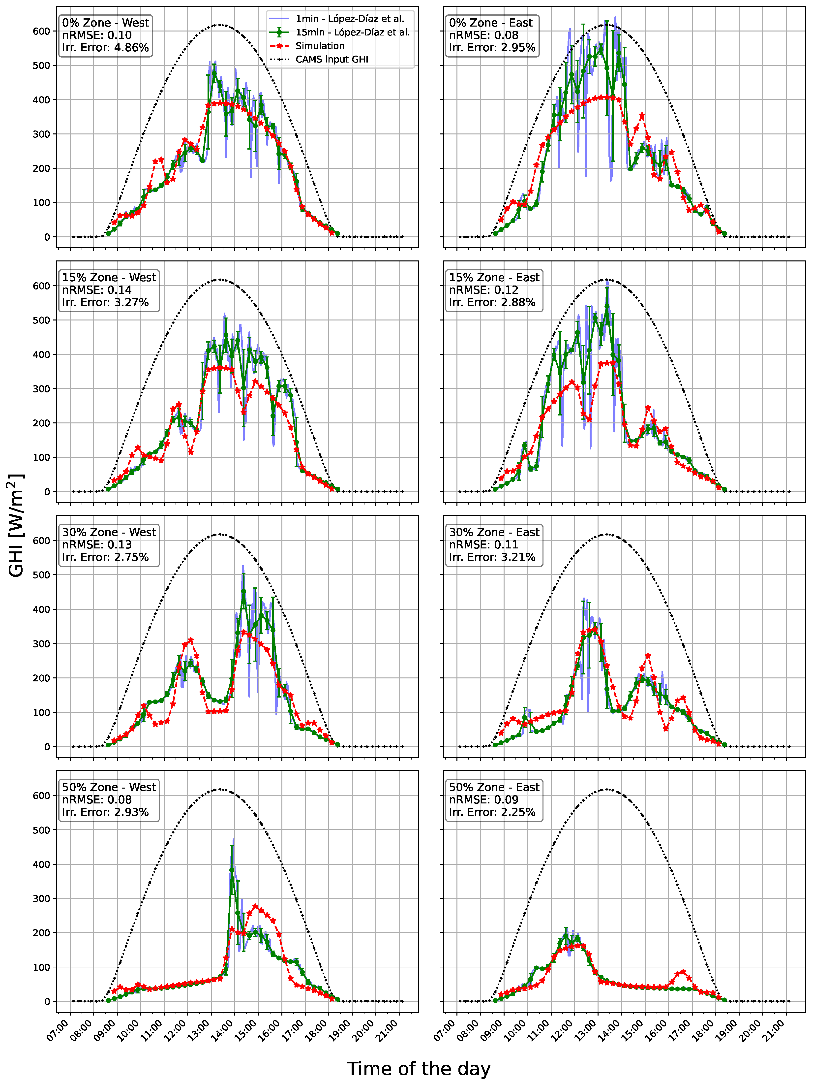
The presented model was validated using experimental data from a Venlo GH study conducted by López-Díaz et al. in Almería, Spain, between 17 September 2014 and 14 May 2015. A sample day, where raw data from the radiation sensors in the experiment were still available, was used to optimize the position of the sensors in the simulation. The method for optimizing the sensor positions was primarily based on a single day of data, which naturally presents certain constraints. However, this approach still provides valuable insights. Factors such as variations in the spectral composition of the incoming irradiance, changes in the solar position affecting the angle of incidence on the GH roof, and fluctuations in the ratio of direct to diffuse radiation could influence the estimated optimal sensor placement. A broader dataset could further enhance the robustness of the methodology by capturing these dynamic conditions more comprehensively. Based on the minimization of the nRMSE of that day, the sensor coordinates were then defined. For that specific day, the simulated irradiance time-series values were compared to the experimentally measured data, and the model demonstrated a radiation error of less than 5%. As mentioned previously, the bias and nRMSE values might be higher for other days, as the sensor positions were fine-tuned based on one day’s data. Over the extended timeframe of the whole crop cycle, the simulated irradiance was on average 2.88 percentage points lower than the experimentally measured data.

The reasons for the deviations in the comparison between the presented localized simulations and the experimental measurements include geometric mismatches, such as discrepancies in the overall GH structure and small misalignments in sensor positioning relative to the GH structure, which are still possible even after the optimization of sensor coordinates. Additionally, the properties of the GH materials can change over time, e.g., plastic coverings may degrade over time, leading to a different transmittance than at the start of their use. The constant exposure to solar radiation and chemical products during cultivation can cause the degradation of GH plastic films [42]. In the Mediterranean region, GH coverings are usually changed every three years due to a decline in their performance and eventual loss of utility. [7]. The study of Abdel-Ghany et al. showed that the transmission of LDPE materials exposed to arid conditions for one year decreased by roughly 32% [58]. In the simulation, plastic cover materials are modeled as uniform surfaces with constant material properties, and such an aging effect is neglected. For the application of the model to the GH experiment in López-Díaz et al., the material definition of the plastic covering was optimized based on the available dataset of one exemplary day and with the information given in [41] to match the experimental results of one crop cycle. In order to improve model accuracy for long-term predictions, given the extended timeframe of GH operations, a temporal evolution of material properties could improve model accuracy. This could be realized in the simulation by gradually adjusting material properties or, as a simplified approach, applying a continuous degradation factor on the assumed plastic transmittance value. However, detailed knowledge of the degradation processes and additional experimental data would be needed to implement such a method.

Furthermore, spontaneous changes in light diffraction can also occur due to the movement of the plastic covering caused by wind or even small holes in the roof, which would further contribute to measurement fluctuations in an experiment but are not included in the simulation. Other potential factors include inhomogeneous soiling of the plastic roof, which can cause variations in irradiance measurements at the same location depending on the sun’s position, as well as sensor soiling due to the GH’s microclimate.

It might be of interest to compare the presented model to the findings of Torrente et al. [34], who also simulated the GH studied by López-Díaz et al., and of Cossu et al. [17], who conducted more general simulations of various north–south-oriented APV GHs. Such a comparison is not directly possible with the presented application of our model due to the differences in the GH types studied, the timeframes of the simulations, and the methodologies used, particularly the averaging of larger areas rather than point-like simulations as in the presented model.

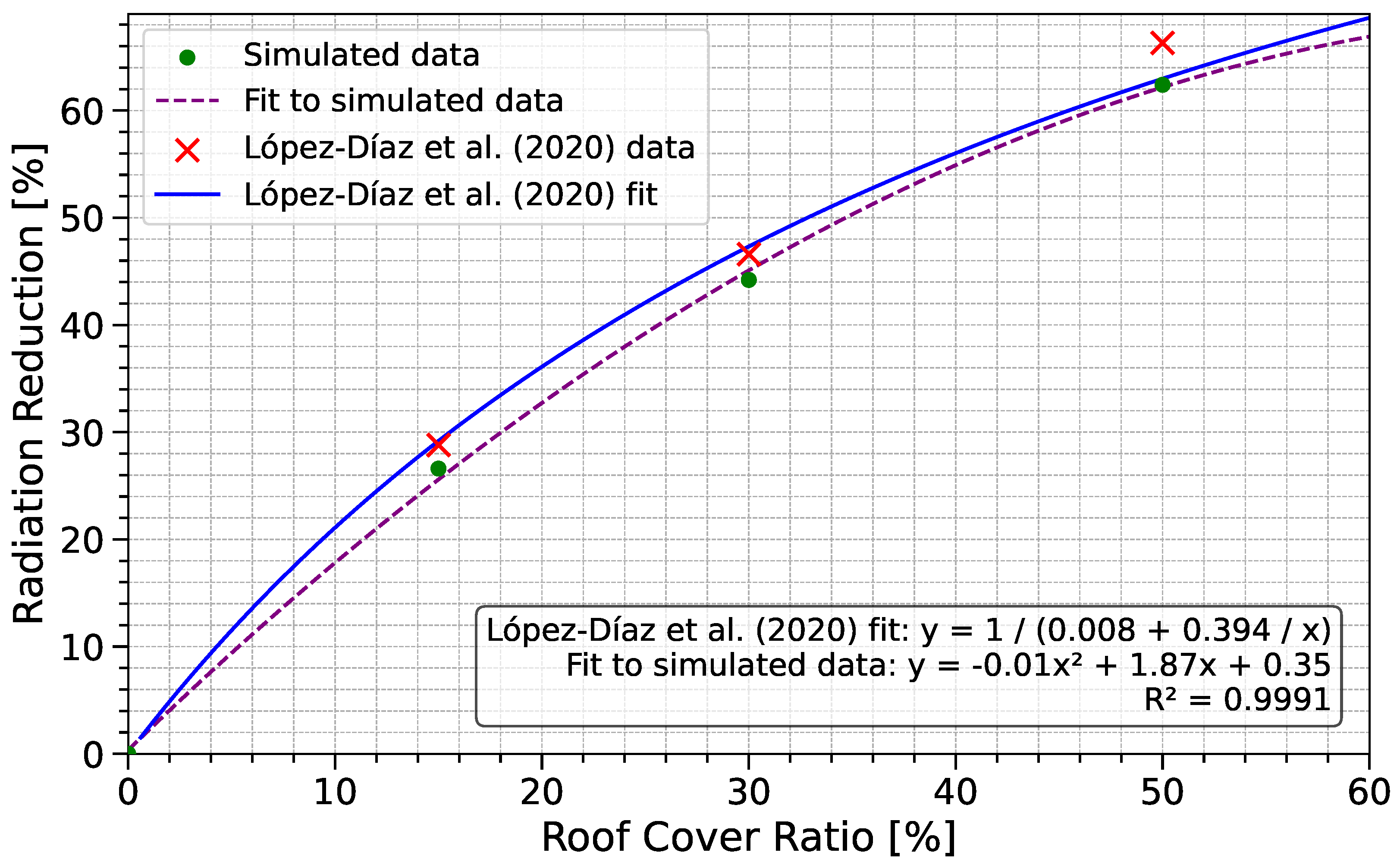
Torrente et al. [34] proposed a method incorporating the transmission of GH plastic dependent on the solar incidence angle. The resulting radiation reduction was calculated by averaging the radiation distribution across the entire GH for each individual shading zone of the experimental setup. Their calculations of the irradiance maps for the experimental GH in López-Díaz et al. were based on representative days for each month taken from a TMY. By integrating these values over time, Torrente et al. estimated both monthly and annual radiation levels for different points inside the GH and provided averaged irradiation maps for the GH. Their findings showed radiation reductions of 11%, 24%, and 32% for 15%, 30%, and 50% shading, respectively. Furthermore, their model predicted lower absolute irradiance values in the 0% shading zone.

Cossu et al. [17] simulated the irradiance distribution for various GH types with different roof cover ratios and estimated the yearly radiation reductions based on the entire GH area. They estimated the annual average values of global solar radiation within GHs equipped with PV modules and evaluated the impact of different PV cover ratios, orientations, and structural parameters on light uniformity and availability over the course of a year. The simulations in their study did not use actual input irradiance data but instead estimated yearly trends based on representative climate data. Their findings reported yearly averaged radiation reductions of 9%, 18%, and 30% for 15%, 30%, and 50% shading, respectively, for north–south-oriented GHs at a height of $1.5$ $\mathrm{m}$.

Both studies focused on estimating spatially averaged irradiance values rather than modeling local light distribution. Their methods can account for the irradiance entering through the GH’s side walls, but they do not resolve the detailed shading patterns created by structural elements and PV modules at specific positions inside the GH. Additionally, their use of annual average irradiance or TMY files means that local variations in environmental conditions are not considered.

Both studies reported radiation reduction values that are generally lower than the theoretical roof cover ratios of the investigated GHs. Possible explanations for this deviation from the here-presented findings include the north–south orientation of the GH, which causes the shadow of the PV modules to fall outside the GH at various times during the crop cycle. Additionally, a considerable fraction of irradiance enters through the side walls. By averaging the irradiance over the entire zone area, the models of Torrente et al. and Cossu et al. account for this additional amount of irradiance. Furthermore, differences in input irradiance data, GH types, and the investigated timeframes prevent a direct comparison between the studies. The presented model incorporates a more detailed representation of the GH structure and cover materials. Actual satellite-derived irradiance data from the time period of the experiment in López-Diaz et al. rather than annual averages or TMY files are used to model the input irradiance conditions. Hence, the climatic conditions of the time period are illustrated more precisely. This presented model makes it possible to highlight the influence of the local environmental conditions, different sun positions, and the shading caused by the GH structure itself.

In principle, the presented model can also be used to generate an averaged overview of different zones. However, the strength and novelty of the model is its ability to perform localized simulations and to visualize the shading effects caused by the PV modules. The model can also simulate the impact of finer structures, such as components of the GH frame and the light transmission through the GH covering plastic, which contribute to a non-uniform irradiance distribution. Furthermore, the simulations can be performed at any point in the virtual scene, such as at a different height or close to the side walls.

Future improvements can include adjusting the temporal resolution for direct coupling with crop models to provide crop-specific yield predictions. Previous studies demonstrated that hourly time steps are sufficient for both crop modeling and energy yield modeling. Perna et al. [59] confirmed that hourly data provide realistic energy yield predictions in various climatic conditions, while Toledo et al. [60] demonstrated that hourly mean values are suitable for modeling solar irradiance in agricultural setups and assessing APV performance. Most crop models operate effectively on a daily or an hourly time scale and could be coupled directly to the presented model. Boote et al. [61] and Jones et al. [62] highlighted that many crop models, such as DSSAT, effectively utilize daily time steps to simulate crop growth by integrating weather inputs, including irradiance. The TOMGRO model of Jones et al. [63] works with hourly time steps to simulate tomato crop development in GHs, making it possible to display the reaction to finer-scale variations in irradiance. However, when using hourly averaged irradiance data, information on short-term fluctuations in irradiance, as presented here, can be lost. Beyond the coupling to specific crop models, the model could also be integrated into a comprehensive framework including an economic yield estimation, e.g., similar to the evaluations of Schallenberg-Rodriguez et al. on a regional scale for the Canary islands [38] or Loh et al. on the national scale for the United States [64].

In this manuscript, our simulation results are compared to the experimental measurements of López-Díaz et al. [41]. The simulation results showed that the line placement of PV modules along the roof of a north– south-oriented GH leads to significant shading periods, as was already proven by the experimentally measured values in the study of López-Diaz et al. [41]. The results from the presented application of the model also indicate that the irradiance distribution inside the GH is not only influenced by the PV shading, but, depending on the position in the GH, the structure itself leads to an inhomogeneous irradiance distribution. For each GH configuration and dependent on the site, different PV configurations might be more beneficial and there is no general, optimal solution for PV placement. This agrees with the experimental studies and pilot sites across Europe, which showed that the design of APV solutions always has to be adapted to location-specific climatic conditions [26]. For GHs, different studies indicate that checkerboard patterns and semi-transparent PV modules improve light uniformity [29,65]. Furthermore, small and fast-moving shade patterns can be more beneficial to plant growth [66]. Nevertheless, the final decision on an APV installation does not consider only the PV array but also the grower’s perspective and the specific characteristics of each GH when assessing whether the reduction in crop yield is adequately compensated by energy savings and other factors [65].

6. Conclusions

In this work, a ray-tracing-based model for simulating the irradiance distribution inside APV GHs is presented. The model offers a novel tool in the decision and design process for APV installations. Digital twins of real-scale GHs are implemented and equipped with a PV pattern in a layout specified by the user. The model takes into account the GH structure and the optical transmission properties of the GH’s cover materials. An integration of satellite-derived irradiance data allows the examination of different locations and timeframes. Hence, the model can produce high-resolution insights into the irradiance distribution, which can then be related to specific crops’ needs. The model can be used to optimize the layout of a PV array on a GH. The practical application of the model would ideally allow potential users, e.g., GH owners considering the integration of a PV system on their GH roof, to create a digital twin of their structure. With the model, they would be able to simulate different PV configurations using real irradiance data without the need for costly and time-consuming experimental studies.

The model was also used in the design process of the APV GH experiment in Kujawa et al. [67], with PV modules arranged in a checkerboard pattern. The experiment incorporated three shading zones with four radiation sensors per zone. The data can be used in a future publication to further evaluate the influence of shading percentage, the layout of the PV modules, the height between the plant canopy and the PV modules, and the irradiance entering from the side walls.

The model can help to realistically plan APV GHs without the need for experimental demonstration. With the model, the layout of the PV modules, but theoretically also the layout of the plants within the GH, can be optimized. Additionally, future studies could explore the effects of temporal and spatial variations in albedo. Expanding the model to investigate APV GHs in regions beyond the Mediterranean region would further enhance its versatility and applicability.