
Construction of Orchard Agricultural Machinery Dispatching Model Based on Improved Beetle Optimization Algorithm


Abstract
1. Introduction
2. Problem Statement and Model Development
2.1. Problem Statement
- The scheduling of each agricultural machine starts from the storage facility, and after completing all operational tasks, it returns to the facility;
- The operations of each agricultural machine are independent of each other;
- The scheduling considers only the same type of agricultural machinery fleet, and the path costs for each machinery unit are the same;
- The scheduling costs are calculated based on distance, without considering the operating costs of the agricultural machinery.
2.2. Model Development
3. Materials and Methods
3.1. Dung Beetle Optimization Algorithm
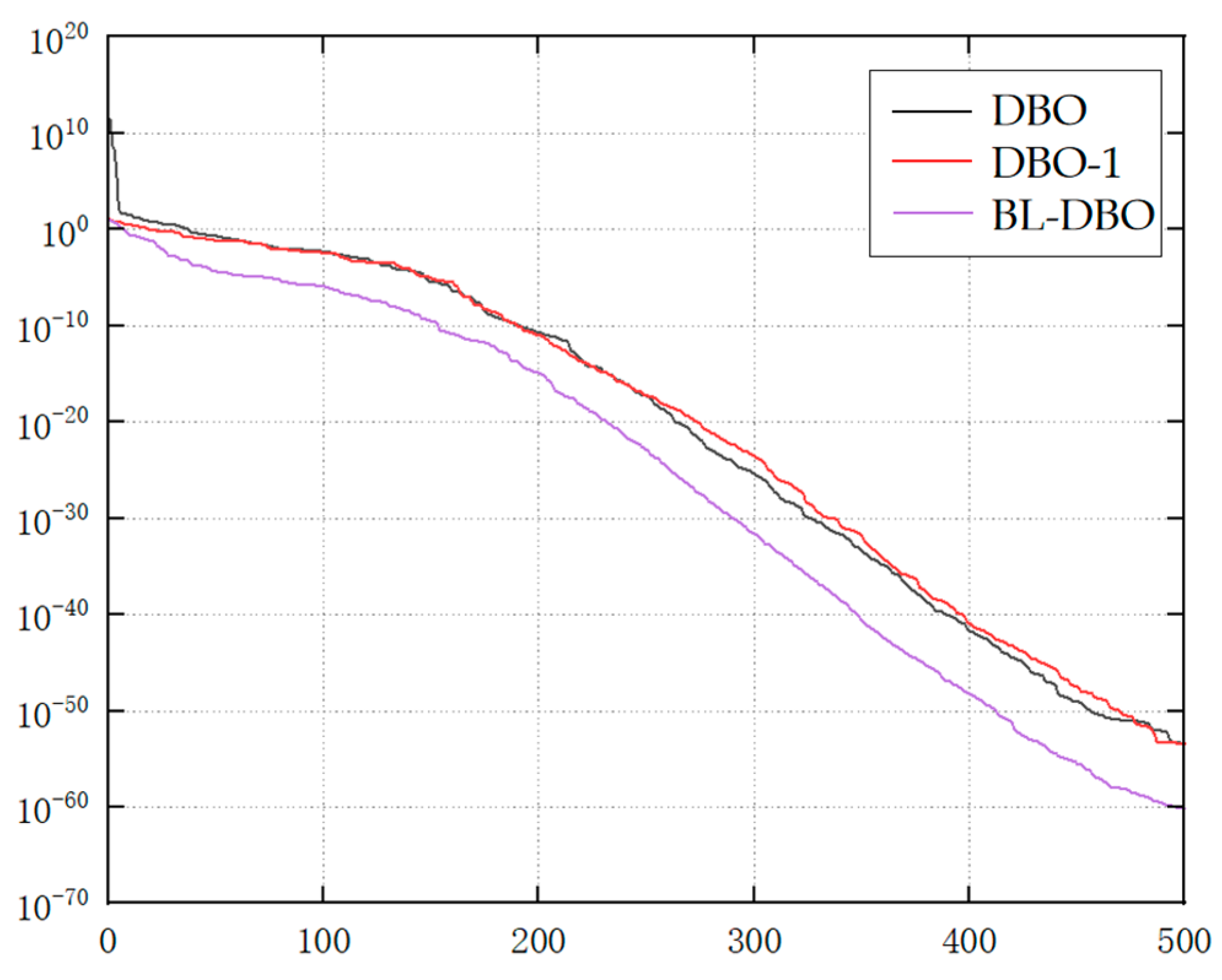
3.2. Improved the Dung Beetle Optimization Algorithm
| Algorithm 1 BL-DBO |
| Establish the initial population and set the parameters number_Dung Beetle = N Max − iter = T Min − Bounds = Lb Max − Bounds = Ub Set the initial positions for the population utilization Equation (20) Establish initial global fitness values using the fitness evaluation Equation (1) While (t < T) do For i = 1:N do If i ∈ rolling_dung_beetle then If τ < 0.9 then # τ ∈ (0, 1) Adjust the position of dung beetle X(i) according to Equation (11) Update the fitness values NewFit[i] based on Equation (1) Else Revise the position of dung beetle X(i) using Equation (13) Recalculate the fitness values NewFit[i] employing Equation (1) End If End If If i ∈ breeding_dung_beetle then Modify the position of dung beetle X(i) based on Equation (24) Renew the fitness values NewFit[i] according to Equation (1) End If If i ∈ foraging_dung_beetle then Adjust the location of dung beetle X(i) using Equation (25) Reevaluate the fitness values NewFit[i] based on Equation (1) End If If i ∈ stealing_dung_beetle then Alter the position of dung beetle X(i) according to Equation (26) Recalculate the fitness values as NewFit[i] using Equation (1) End If Greedy choice If NewFit[i] < Fitness then Fit[i] = NewFit[i] End If End For t = t + 1 End While Provide the global optimal position, BestPosition, and its corresponding fitness value, BestFitness |
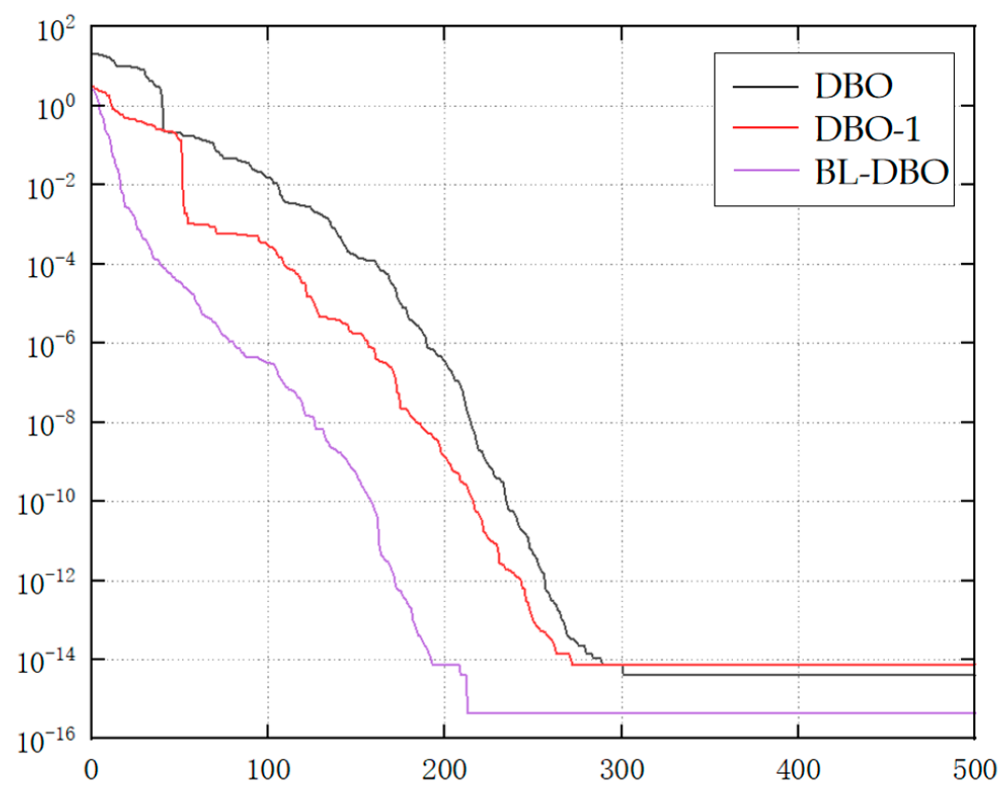
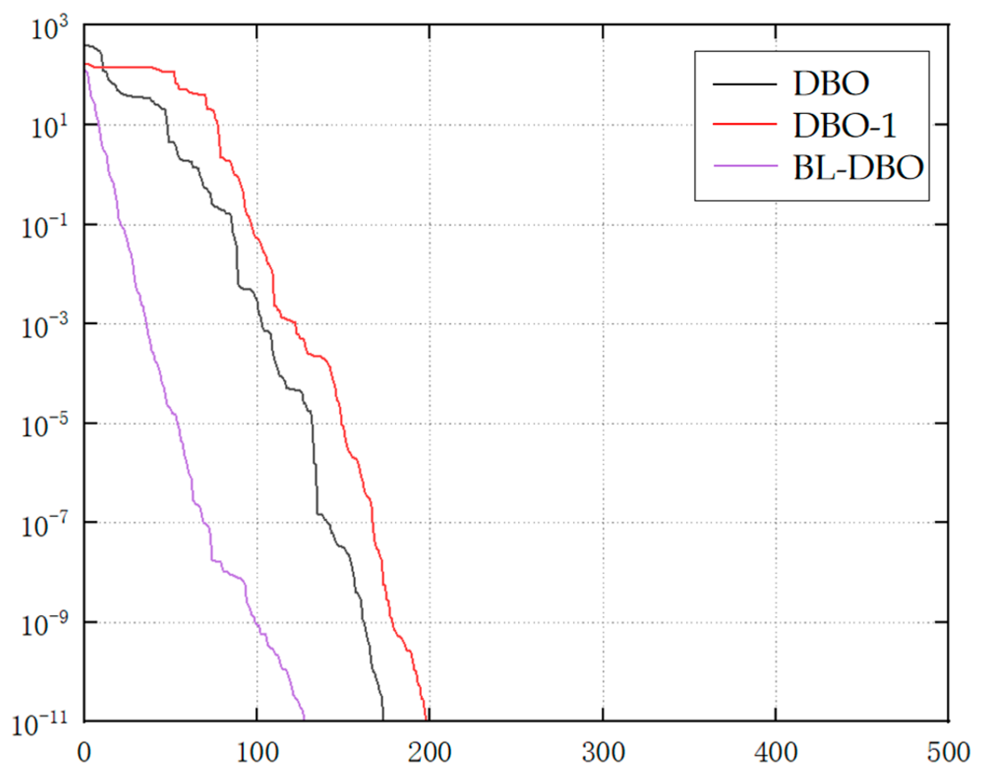
3.3. Ablation Test
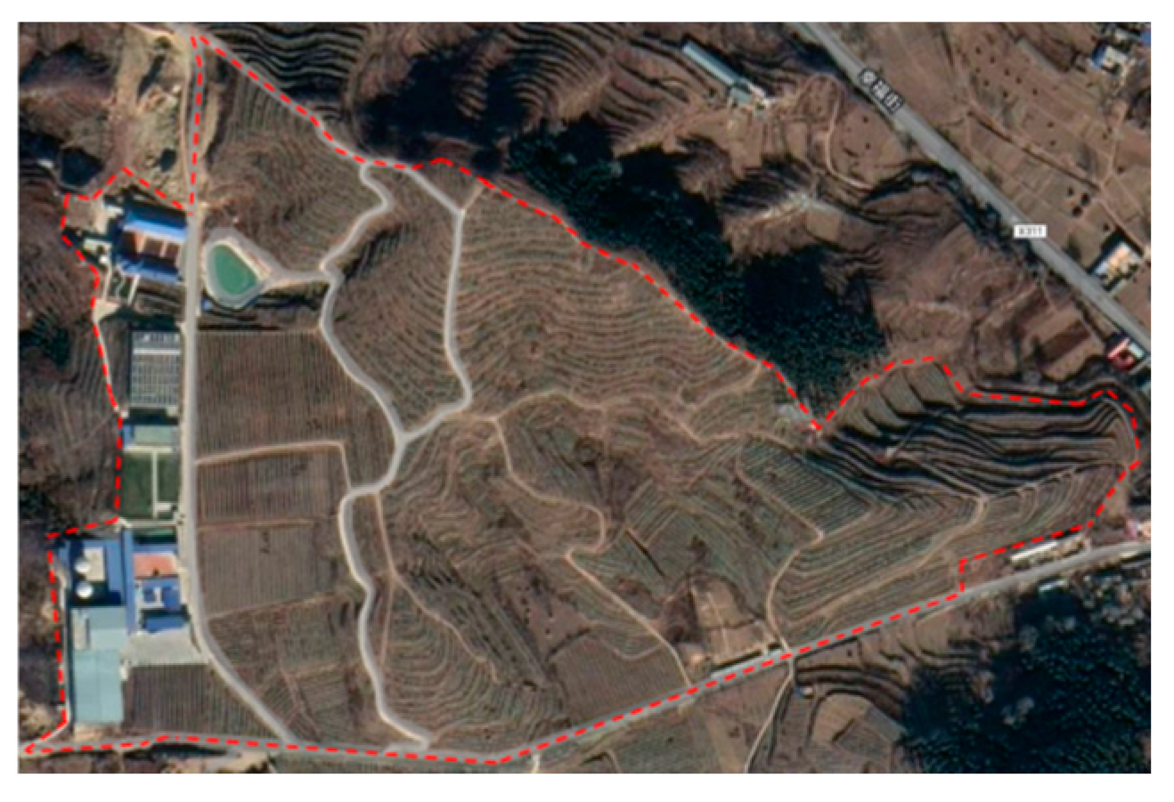
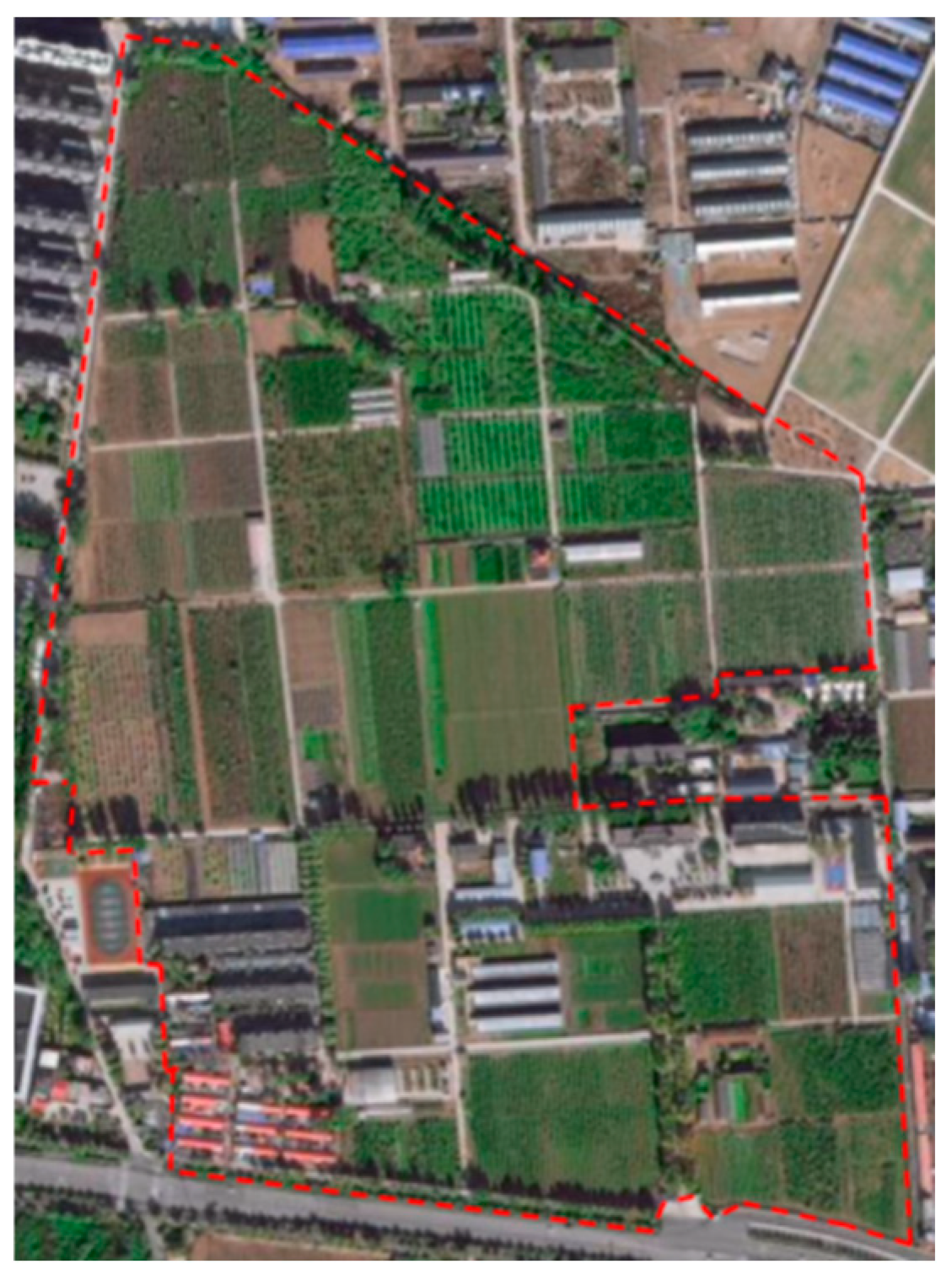
3.4. Experimental Materials
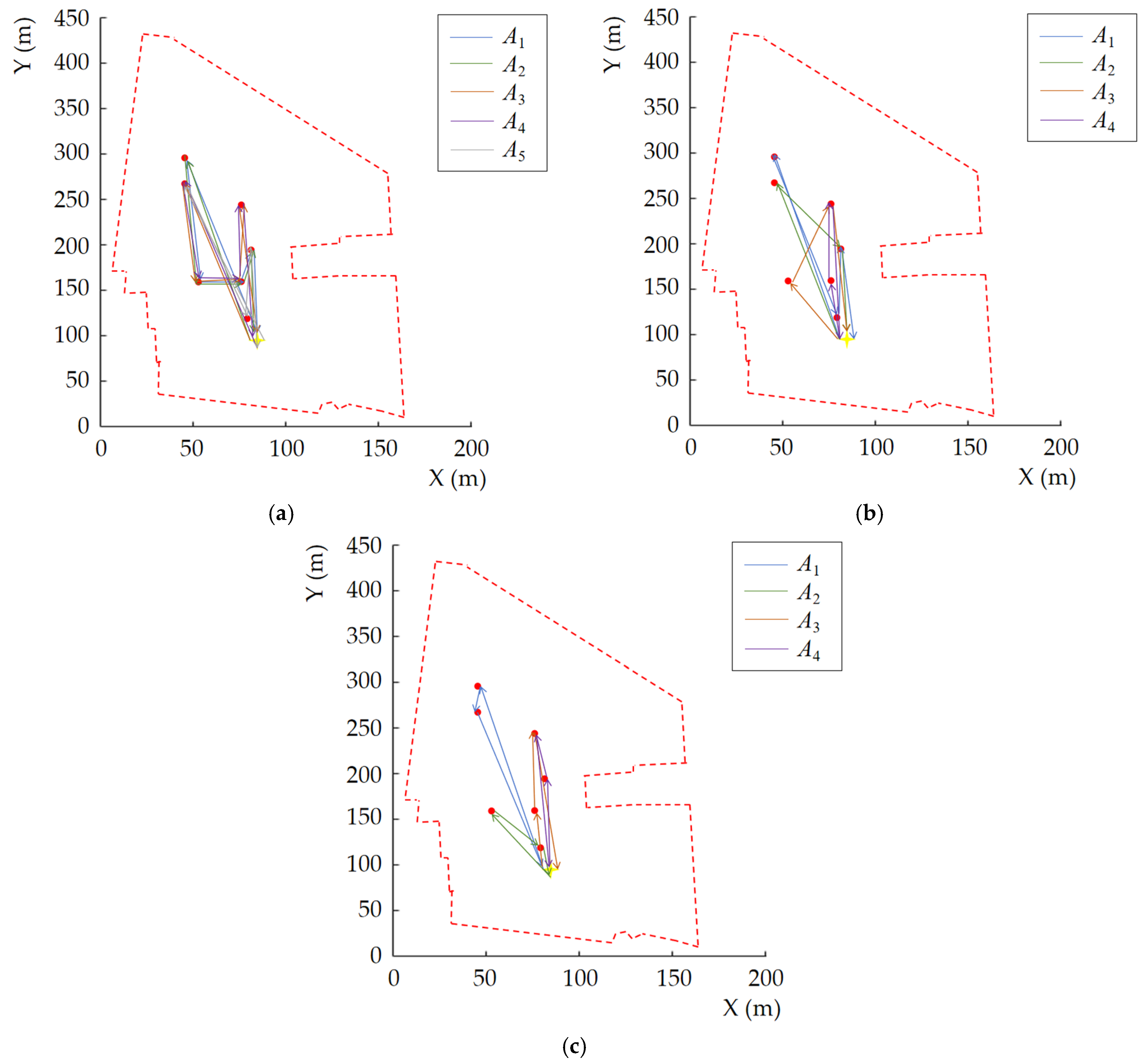
4. Results and Discussion
5. Conclusions
Author Contributions
Funding
Data Availability Statement
Conflicts of Interest
References
- Qian, L.; Lu, H.; Gao, Q.; Lu, H. Household-owned farm machinery vs. outsourced machinery services: The impact of agricultural mechanization on the land leasing behavior of relatively large-scale farmers in China. Land Use Policy 2022, 115, 106008. [Google Scholar] [CrossRef]
- Chakraborty, S.; Elangovan, D.; Govindarajan, P.L.; ELnaggar, M.F.; Alrashed, M.M.; Kamel, S. A comprehensive review of path planning for agricultural ground robots. Sustainability 2022, 14, 9156. [Google Scholar] [CrossRef]
- Sharma, V.; Tripathi, A.K.; Mittal, H. Technological revolutions in smart farming: Current trends, challenges & future directions. Comput. Electron. Agric. 2022, 201, 107217. [Google Scholar]
- Albiero, D.; Garcia, A.P.; Umezu, C.K.; Paulo, R.L. Swarm robots in mechanized agricultural operations: A review about challenges for research. Comput. Electron. Agric. 2022, 193, 106608. [Google Scholar] [CrossRef]
- Huang, X.M.; Ding, Y.C.; Zong, Y.W.; Liao, Q.X. Research on the Turning Mode and Path Generation Algorithm of Agricultural Machinery Operation Headland. In Proceedings of the 2011 Annual Academic Conference of China Agricultural Engineering Society, Changsha, China, 21–24 October 2011; pp. 1–6. [Google Scholar]
- Wang, D.; Wang, G.; Sun, S.; Lu, X.; Liu, Z.; Wang, L.; Wang, K. Research Progress on Cuttings of Malus Rootstock Resources in China. Horticulturae 2024, 10, 217. [Google Scholar] [CrossRef]
- Patle, B.K.; Pandey, A.; Parhi, D.R.K.; Jagadeesh, A.J.D.T. A review: On path planning strategies for navigation of mobile robot. Def. Technol. 2019, 15, 582–606. [Google Scholar] [CrossRef]
- Sun, J.; Chen, Z.; Song, R.; Fan, S.; Han, X.; Zhang, C.; Wang, J.; Zhang, H. An intelligent self-propelled double-row orchard trenching and fertilizing machine: Modeling, evaluation, and application. Comput. Electron. Agric. 2025, 229, 109818. [Google Scholar] [CrossRef]
- Bochtis, D. Planning and Control of a Fleet of Agricultural Machines for Optimal Management of Field Operations. Ph.D. Thesis, Aristotle University of Thessaloniki, Thessaloniki, Greece, 2008. [Google Scholar]
- Bochtis, D.; Griepentrog, H.W.; Vougioukas, S.; Busato, P.; Berruto, R.; Zhou, K. Route planning for orchard operations. Comput. Electron. Agric. 2015, 113, 51–60. [Google Scholar] [CrossRef]
- Liu, L.; Wang, X.; Xie, J.; Wang, X.; Liu, H.; Li, J.; Wang, P.; Yang, X. Path planning and tracking control of orchard wheel mower based on BL-ACO and GO-SMC. Comput. Electron. Agric. 2025, 228, 109696. [Google Scholar] [CrossRef]
- Ye, Y.; He, L.; Wang, Z.; Jones, D.; Hollinger, G.A.; Taylor, M.E.; Zhang, Q. Orchard manoeuvring strategy for a robotic bin-handling machine. Biosyst. Eng. 2018, 169, 85–103. [Google Scholar] [CrossRef]
- Mia, M.J.; Massetani, F.; Murri, G.; Facchi, J.; Monaci, E.; Amadio, L.; Neri, D. Integrated weed management in high density fruit orchards. Agronomy 2020, 10, 1492. [Google Scholar] [CrossRef]
- Bochtis, D.D.; Sørensen, C.G.; Busato, P. Advances in agricultural machinery management: A review. Biosyst. Eng. 2014, 126, 69–81. [Google Scholar] [CrossRef]
- Yang, H.; Wang, L.; Liu, L.; Huang, H.; Ding, C. Model construction and application of agricultural machinery cross-region scheduling based on blockchain. Trans. Chin. Soc. Agric. Eng. (Trans. CSAE) 2022, 38, 31–40. [Google Scholar]
- Xue, J.; Shen, B. Dung beetle optimizer: A new meta-heuristic algorithm for global optimization. J. Supercomput. 2023, 79, 7305–7336. [Google Scholar] [CrossRef]
- Wei, X.R.; Bai, W.L.; Liu, L.; Li, Y.M.; Wang, Z.Y. A hybrid dung beetle optimization algorithm with simulated annealing for the numerical modeling of asymmetric wave equations. Appl. Geophys. 2024, 21, 513–527. [Google Scholar] [CrossRef]
- Yang, X.; Cui, Y.; Jia, L.; Sun, Z.; Zhang, P.; Zhao, J.; Wang, R. Parameter identification of PMSM based on dung beetle optimization algorithm. Arch. Electr. Eng. 2023, 72, 1055–1072. [Google Scholar]
- Li, Y.; Sun, K.; Yao, Q.; Wang, L. A dual-optimization wind speed forecasting model based on deep learning and improved dung beetle optimization algorithm. Energy 2024, 286, 129604. [Google Scholar] [CrossRef]
- Wang, X.; Wei, Y.; Guo, Z.; Wang, J.; Yu, H.; Hu, B. A Sinh–Cosh-Enhanced DBO Algorithm Applied to Global Optimization Problems. Biomimetics 2024, 9, 271. [Google Scholar] [CrossRef] [PubMed]
- Tang, C.; Li, W.; Han, T.; Yu, L.; Cui, T. Multi-Strategy Improved Harris Hawk Optimization Algorithm and Its Application in Path Planning. Biomimetics 2024, 9, 552. [Google Scholar] [CrossRef] [PubMed]
- Mai, C.; Zhang, L.; Chao, X.; Hu, X.; Wei, X.; Li, J. A novel MPPT technology based on dung beetle optimization algorithm for PV systems under complex partial shade conditions. Sci. Rep. 2024, 14, 6471. [Google Scholar] [CrossRef] [PubMed]
- Huang, H.; Yao, Z.; Wei, X.; Zhou, Y. Twin support vector machines based on chaotic mapping dung beetle optimization algorithm. J. Comput. Des. Eng. 2024, 11, 101–110. [Google Scholar] [CrossRef]
- Zhang, D.; Zhang, Z.; Zhang, J.; Zhang, T.; Zhang, L.; Chen, H. UAV-assisted task offloading system using dung beetle optimization algorithm & deep reinforcement learning. Ad Hoc Netw. 2024, 156, 103434. [Google Scholar]
- Zhu, F.; Li, G.; Tang, H.; Li, Y.; Lv, X.; Wang, X. Dung beetle optimization algorithm based on quantum computing and multi-strategy fusion for solving engineering problems. Expert Syst. Appl. 2024, 236, 121219. [Google Scholar] [CrossRef]
- Wang, Z.; Huang, L.; Yang, S.; Li, D.; He, D.; Chan, S. A quasi-oppositional learning of updating quantum state and Q-learning based on the dung beetle algorithm for global optimization. Alex. Eng. J. 2023, 81, 469–488. [Google Scholar] [CrossRef]
- Fang, R.; Zhou, T.; Yu, B.; Li, Z.; Ma, L.; Zhang, Y. Dung Beetle Optimization Algorithm Based on Improved Multi-Strategy Fusion. Electronics 2025, 14, 197. [Google Scholar] [CrossRef]
- Arora, S.; Anand, P. Chaotic grasshopper optimization algorithm for global optimization. Neural Comput. Appl. 2019, 31, 4385–4405. [Google Scholar] [CrossRef]


| Function | Name | Dimension | Range | Optimal |
|---|---|---|---|---|
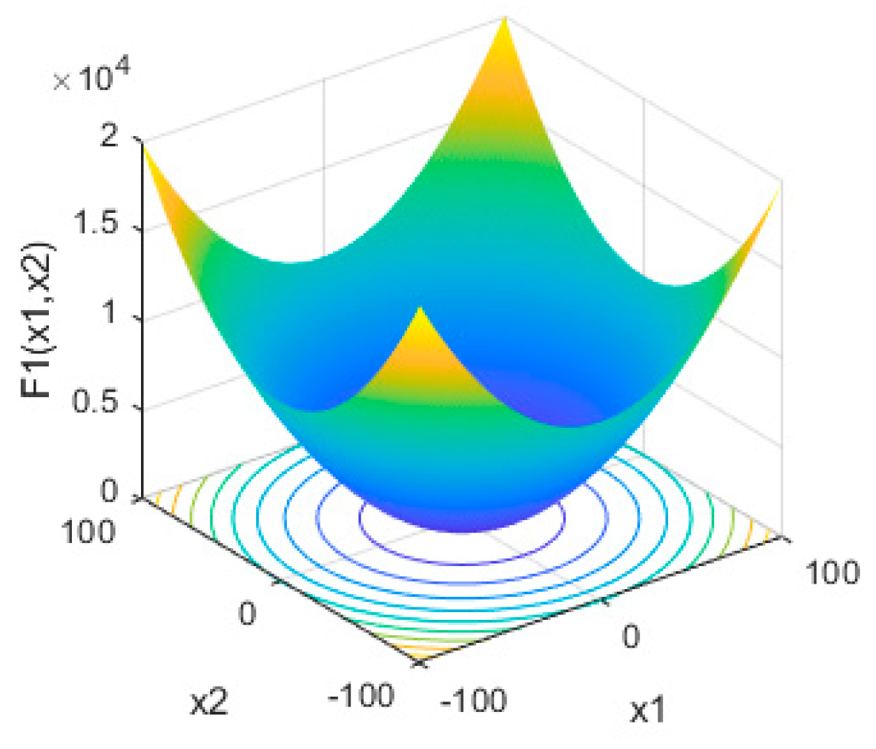
| F1 | Sphere | 30 | [−100, 100] | 0 |
| F2 | Schwefel 2.22 | 30 | [−10, 10] | 0 |
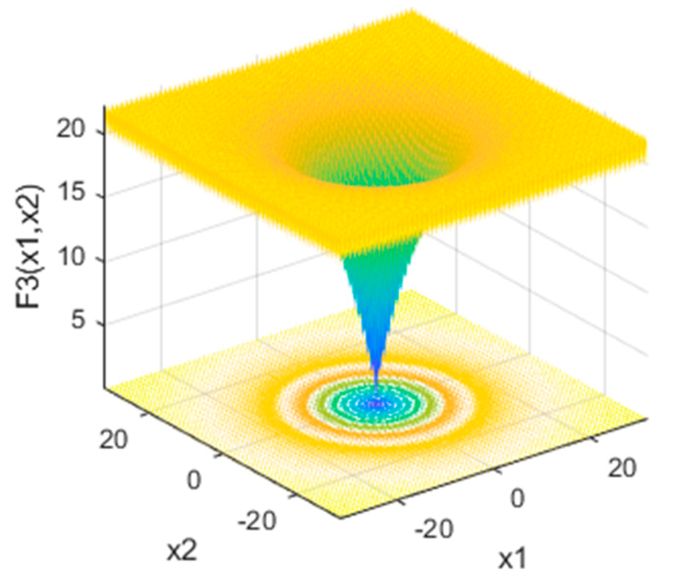
| F3 | Ackley | 30 | [−32, 32] | 0 |
| F4 | Rastrigin | 30 | [−5.12, 5.12] | 0 |
| Base | Factory Coordinates | Small Park Number | Entrance and Exit Coordinates | Quantity of Agricultural Machinery Required per Unit Time |
|---|---|---|---|---|
| Shunnong Fruit Modern Agricultural Park | (35.25, 101) | f1 | (95.6, 286.7) | 2 |
| f2 | (49.36, 193.77) | 3 | ||
| f3 | (53.77, 148.22) | 2 | ||
| f4 | (52.98, 54.33) | 2 | ||
| f5 | (99.32, 152.64) | 1 | ||
| f6 | (112.43, 163.27) | 4 | ||
| f7 | (112.69, 204.89) | 3 | ||
| f8 | (129.32, 221.36) | 4 | ||
| Shijiazhuang Fruit Tree Research Institute | (80.22, 93.62) | f9 | (48.32, 296.11) | 2 |
| f10 | (48.14, 267.13) | 3 | ||
| f11 | (51.36, 154.78) | 4 | ||
| f12 | (79.65, 116.42) | 1 | ||
| f13 | (76.54, 153.85) | 4 | ||
| f14 | (81.93, 193.62) | 4 | ||
| f15 | (77.35, 246.21) | 3 |
| Method | Farm Machinery Number | f1 | f2 | f3 | f4 | f5 | f6 | f7 | f8 |
|---|---|---|---|---|---|---|---|---|---|
| Human experience | A1 | √ 1 | √ | √ | |||||
| A2 | √ | √ | √ | ||||||
| A3 | √ | √ | √ | ||||||
| A4 | √ | √√ | √ | ||||||
| A5 | √ | √√ | √ | ||||||
| A6 | √√ | √√ | |||||||
| DBO | A1 | √ | √ | √ | √√ | ||||
| A2 | √ | √ | √ | √√ | |||||
| A3 | √ | √ | √ | √ | |||||
| A4 | √ | √ | √ | √ | |||||
| A5 | √ | √ | √ | ||||||
| BL-DBO | A1 | √√ | √√√ | ||||||
| A2 | √√ | √√ | √ | ||||||
| A3 | √√√√ | √√ | |||||||
| A4 | √√√ | √√ |
| Method | Farm Machinery Number | f1 | f2 | f3 | f4 | f5 | f6 | f7 |
|---|---|---|---|---|---|---|---|---|
| Human experience | A1 | √ 1 | √ | √ | √ | |||
| A2 | √ | √ | √ | √ | ||||
| A3 | √ | √ | √ | √√ | ||||
| A4 | √ | √ | √ | √ | ||||
| A5 | √ | √ | √√ | |||||
| DBO | A1 | √√ | √ | √√ | ||||
| A2 | √√√ | √√ | ||||||
| A3 | √√√√ | √√ | ||||||
| A4 | √√√√ | √ | ||||||
| BL-DBO | A1 | √√ | √√√ | |||||
| A2 | √√√√ | √ | ||||||
| A3 | √√√√ | √√ | ||||||
| A4 | √√√√ | √ |
| Base | Farm Machinery Number | Human Experience | DBO | BL-DBO |
|---|---|---|---|---|
| Shunnong Fruit Modern Agricultural Park | A1 | 2 | 3 | 1 |
| A2 | 2 | 3 | 2 | |
| A3 | 2 | 3 | 1 | |
| A4 | 2 | 3 | 1 | |
| A5 | 2 | 3 | - | |
| A6 | 1 | - | - | |
| Shijiazhuang Fruit Tree Research Institute | A1 | 3 | 2 | 1 |
| A2 | 3 | 1 | 1 | |
| A3 | 3 | 1 | 1 | |
| A4 | 3 | 1 | 1 | |
| A5 | 2 | - | - |
Disclaimer/Publisher’s Note: The statements, opinions and data contained in all publications are solely those of the individual author(s) and contributor(s) and not of MDPI and/or the editor(s). MDPI and/or the editor(s) disclaim responsibility for any injury to people or property resulting from any ideas, methods, instructions or products referred to in the content. |
© 2025 by the authors. Licensee MDPI, Basel, Switzerland. This article is an open access article distributed under the terms and conditions of the Creative Commons Attribution (CC BY) license (https://creativecommons.org/licenses/by/4.0/).
Share and Cite
Liu, L.; Liu, H.; Li, J.; Wang, P.; Yang, X. Construction of Orchard Agricultural Machinery Dispatching Model Based on Improved Beetle Optimization Algorithm. Agronomy 2025, 15, 323. https://doi.org/10.3390/agronomy15020323
Liu L, Liu H, Li J, Wang P, Yang X. Construction of Orchard Agricultural Machinery Dispatching Model Based on Improved Beetle Optimization Algorithm. Agronomy. 2025; 15(2):323. https://doi.org/10.3390/agronomy15020323
Chicago/Turabian StyleLiu, Lixing, Hongjie Liu, Jianping Li, Pengfei Wang, and Xin Yang. 2025. "Construction of Orchard Agricultural Machinery Dispatching Model Based on Improved Beetle Optimization Algorithm" Agronomy 15, no. 2: 323. https://doi.org/10.3390/agronomy15020323
APA StyleLiu, L., Liu, H., Li, J., Wang, P., & Yang, X. (2025). Construction of Orchard Agricultural Machinery Dispatching Model Based on Improved Beetle Optimization Algorithm. Agronomy, 15(2), 323. https://doi.org/10.3390/agronomy15020323