Article

The Impact of Climate Change on Chorthippus dubius (Zubovski, 1898) Distribution in Alpine Grassland—A Case Study in the Qilian Mountain National Park, China

1
Key Laboratory of Grassland Ecosystem of Ministry of Education, College of Pratacultural Science, Gansu Agricultural University, Lanzhou 730070, China
2
Qinghai Service and Guarantee Center of Qilian Mountain National Park, Xining 810001, China
3
Key Laboratory of Oasis Ecology of Ministry of Education, College of Ecology and Environment, Xinjiang University, Urumqi 830046, China
4
State Key Laboratory of Herbage Improvement and Grassland Agro-Ecosystems, College of Pastoral Agriculture Science and Technology, Lanzhou University, Lanzhou 730000, China
*
Author to whom correspondence should be addressed.
These authors contributed equally to this work.
Agronomy 2025, 15(12), 2728; https://doi.org/10.3390/agronomy15122728
Submission received: 24 October 2025 / Revised: 22 November 2025 / Accepted: 24 November 2025 / Published: 27 November 2025
(This article belongs to the Section Grassland and Pasture Science)

Abstract

Alpine grassland is extremely sensitive to climate change and external interference, and it does not easily recover once damaged. Grasshopper outbreaks pose a serious threat to grassland ecosystem health and to the sustainable development of animal husbandry. However, most of the current grasshopper hazard studies focus on tropical, temperate, and desert areas, and there is still a lack of understanding of the spatial and temporal variation in the Qinghai–Tibet Plateau. Hence, the alpine grassland in the Qilian National Park (located in the eastern Qinghai–Tibet Plateau) was selected as the study area to investigate the primary environmental drivers, construct optimal ecological niche models, and evaluate the impact of climate change on the inhabitable areas of the dominant species Chorthippus dubius (Zubovski, 1898), abbreviated as C. dubius. The results indicate that (1) temperature seasonality, slope, and precipitation were the main influence factors for the distribution of C. dubius; (2) among the 10 ecological niche models, the random forest (RF) model exhibited the highest performance, achieving kappa, TSS, and ROC values of 0.86, 0.90, and 0.98, respectively; and (3) in the future climate scenario (SSP126–SSP585), most of the lower presence probability area (less than 20%) will be transformed into other types, affecting 93.17% of its current area. In addition, the presence probability increased from northwest to southeast gradually. This study clarified the spatial and temporal variation in C. dubius presence probability and its response to climate change, providing a scientific basis for grasshopper control and grassland management in Qilian Mountain National Park.

1. Introduction

Grasshopper outbreaks, as well as floods and droughts, are the major disasters in human history, posing a serious threat to agriculture and animal husbandry. With the exception of Antarctica, grasshopper outbreaks can occur on all continents around the world; affecting the livelihoods of nearly 10% of the global population, grasshopper outbreaks are considered one of the most serious global agricultural problems [1,2]. Grasshoppers are typical herbivorous insects with relatively large, winged populations, belonging to the suborder Caelifera of the order Orthoptera. Approximately 10,000 known species of locust and grasshopper are distributed in tropical and temperate grasslands and desert areas worldwide [3]. In China, about 200 locust and grasshopper species are found in grasslands, of which around 20 pose a threat to grassland ecosystem health [4]. Grasshoppers influence grassland growth by feeding on green vegetation. Generally, scattered populations do not cause significant damage to grasslands; on the contrary, they can even play an important role in food chains and nutrient cycling within the grassland ecosystem. When they gather in large groups, grasshoppers can cause extensive damage to grassland, posing a great threat to livestock and other animals living on the grassland [5,6]. However, the life cycle of grasshoppers is influenced by multiple environmental factors, including temperature, precipitation, altitude, topography, and soil type. Among these, temperature and precipitation are key factors. They jointly regulate embryonic development, survival, and hatching of eggs (such as through spring warming and moderate precipitation) [7], directly determine the developmental rate and number of generations of nymphs (summer sustained warming and localized heavy rainfall) [3,8], and ultimately mark the end of the life cycle with autumn cooling and winter frost [9].
The Qinghai–Tibet Plateau encompasses 83% of the global area above an elevation of 4000 m. Alpine grassland is the primary land cover type. The health of the alpine grassland ecosystem is not only vital for the development of local animal husbandry and water conservation, but also for regulating the regional climate, carbon cycling, and protecting biodiversity [10,11,12,13]. Alpine grassland is highly sensitive to external interference, and the ecological environment does not easily recover in a short period once damaged, due to its high altitude and oxygen-deprived environment [14,15]. Grasshopper plagues are one of the major natural disasters that occur on the alpine grassland of the Qinghai–Tibet Plateau. For example, about 1600 km2 and 5000 km2 of alpine grassland suffer from grasshopper outbreaks in Tibet and Qinghai provinces each year, respectively. The mean grasshopper density can reach 150–200 head/m2 during an outbreak, with a maximum density of 1000 head/m2 [16]. Outbreaks of grasshoppers can significantly reduce vegetation cover and plant biomass, thereby exposing the soil, altering species composition, and potentially destabilizing local grassland communities [17,18]. In recent years, with intensified climate change and human activities in alpine grassland, the frequency of insect pest outbreaks is increasing, which poses a serious threat to the development of animal husbandry and ecosystem health [19]. However, most grasshopper hazard studies are focused on tropical, temperate, and desert regions, and there is still a lack of understanding of the current status and spatial and temporal variation in grasshopper hazards in the Qinghai–Tibet Plateau under future climate change [19,20].
Qilian Mountain National Park is located in the central region of the Eurasian continent, at the junction of the Qinghai–Tibet Plateau, Inner Mongolia Plateau, and Loess Plateau. It is one of the most important ecological security barriers in western China [19,21]. Alpine grassland is one of the main types of vegetation in Qilian Mountain National Park, covering 90% of the total area. In recent years, due to climate changes and human activities, approximately 90% of the grassland in the Qilian Mountain National Park has been degraded to various degrees. Grasshopper plagues are one of the main natural disasters in Qilian Mountain National Park, and they could be the cause of the grassland degradation. There are 10 species of grasshoppers in the Qilian Mountain National Park, which has seriously affected the health of grassland ecosystems and sustainable development of the economy [22,23]. Lv et al. analyzed the main environmental influence factors of alpine grassland grasshoppers in Qilian Mountain National Park and classified the inhabitable areas based on field observation data and corresponding environmental factors. The results showed that precipitation, radiation, grassland biomass, soil, and temperature are the main influence factors for grasshopper growth and development [22]. Although the distribution area of grasshoppers in Qilian Mountain National Park is relatively small at present, it is unclear whether the area of grasshopper distribution will increase significantly under climate warming and humidification in future.
Therefore, based on grasshopper field observation data collected between 2000 and 2022, Chorthippus dubius (Zubovski, 1898), abbreviated as C. dubius, is identified as a pest grasshopper and was selected as the target species. Along with corresponding climate, soil, terrain, and grassland biomass data in Qilian Mountain National Park, we employed the BIOMOD2 framework to obtain the optimal ecological niche model for C. dubius. This study provides a scientific basis for predicting and managing C. dubius disasters in the face of climate change and also provides a theoretical basis for ecological environment protection and sustainable development of Qilian Mountain National Park.

2. Materials and Methods

2.1. Study Area

The study area, which is part of Qilian Mountain National Park in Qinghai Province (36.8926–39.2110° N; 96.1380–102.6405° E), is located at the northeast edge of the Qinghai–Tibet Plateau and north of Qinghai Province (Figure 1). The study area includes four counties (Menyuan, Tianjun, Gangcha, and Qilian) and one city (Delingha). The average altitude is over 4000 m, with an average annual temperature below 4 °C. The extreme highest and lowest temperatures are 37.6 °C and −35.8 °C, respectively. The average annual precipitation is 400 mm. Due to the wide distribution of glaciers and permafrost, glacial meltwater is an important source of water in the study area. It has a typical high-altitude continental climate, with abundant sunshine (2500–3300 annual sunshine hours) and intense solar radiation (a total solar radiation of 5916–15,000 megajoules per square meter). Grassland is the most important land cover type in the study area, covering 90% of the total area. Nine grassland types are present in the study area, including alpine meadows, mountain meadows, lowland meadows, alpine meadow steppes, alpine steppes, alpine deserts, warm grasslands, warm desert grasslands, and warm deserts.

2.2. Field Observation

Field observation was performed during the peak grass growing season (June to August) between 2000 and 2022. Observation sites were designed based on the grassland vegetation types and spatial distribution of grasshoppers. The size of the observation sites is 250 m × 250 m, which corresponds to the size of a Moderate Resolution Imaging Spectroradiometer (MODIS) image pixel (with a spatial resolution of 250 × 250 m). Each observation site was selected based on the following criteria: (1) a 5 km horizontal distance was used between every two sites with similar homogeneity of vegetation and land use; (2) similar geomorphology and grassland types were adopted in the same sites; and (3) three to five sub-observation sites (30 m × 30 m) were randomly selected in each site for grasshopper species and density observation.
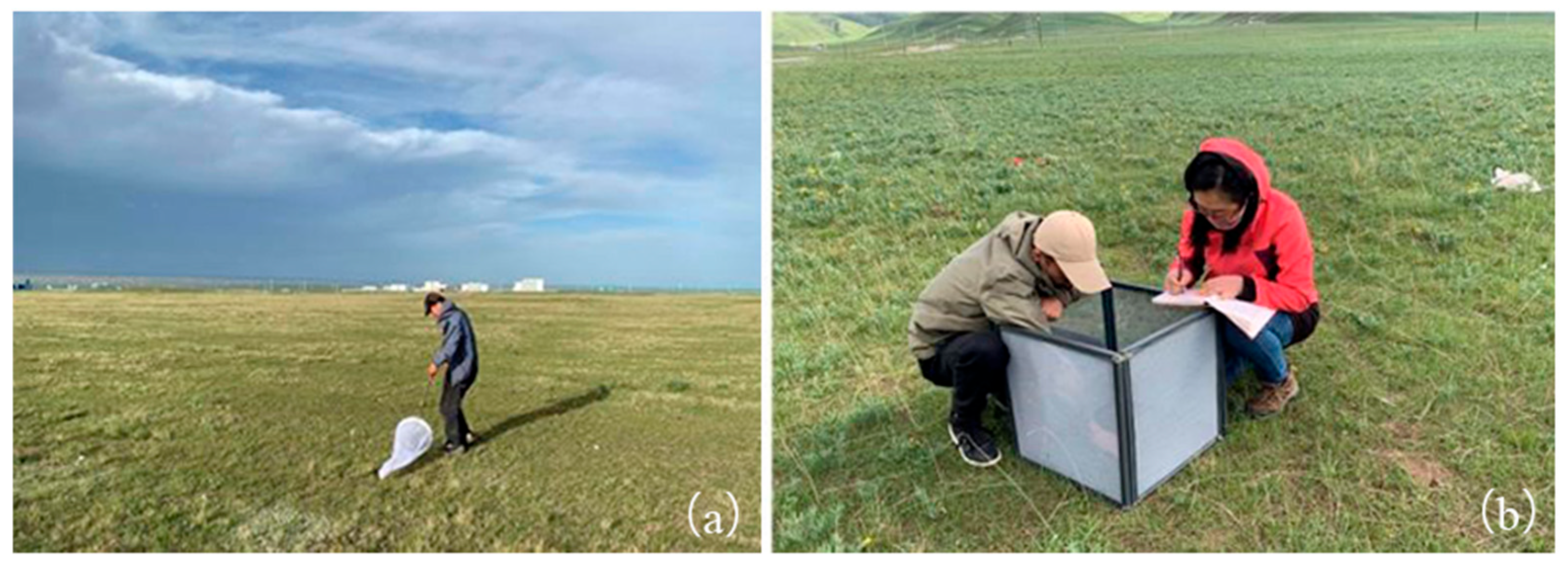
The sweep-net method was employed to survey the grasshopper species. One transect was set up in each sub-observation site. Observers walked along each transect at approximately 0.5 m/s, sweeping the net 180° to either side to complete one sweep. Ten sweeps constituted one sampling unit, and five such sampling units were collected per transect. Finally, the species of all captured grasshoppers were recorded (Figure 2a). The enclosure method was employed to survey the grasshopper density. In each sub-observation site, a “Z”-shaped transect was used to set up 10 quadrats, each with an area of 0.5 m2. The mean density value of 10 quadrats was used to represent the density of the corresponding observation site (Figure 2b). After completing the field surveys, each specimen was immediately placed in labeled vials, with the labels indicating the collection site and date, and then stored in 70% ethanol for preservation. In the laboratory, specimens were sorted and identified at the species level using morphological characteristics under a stereomicroscope. Identification relied on standard taxonomic keys for Orthoptera, which were sourced from the well-established taxonomic literature and databases, with particular attention to features such as body size, coloration, wing venation, and genitalia structure.
Finally, a total of 298 sites were investigated in the study area, and 10 grasshopper species were identified: Bryodema miramae, Bryodema luctuosum, Bryodema hyalinala, Angaracris barabensis, Chorthippus qingzangensis, Chorthippus fallax, Chorthippus dubius, Chorthippus huchengensis, Myrmeleotettix palpalis, and Chorthippus albonemus. Among these species, Chorthippus dubius (C. dubius) exhibited the widest distribution and the highest population density in the Qilian Mountain National Park. Hence, C. dubius was selected as the focal species to explore its spatial distribution, influencing factors, and responses to climate change.

2.3. Environmental Factors and Data Preprocessing

The climate data was downloaded from the Climatic Research Unit at the University of East Anglia, and bias correction was performed using WorldClim 2.1 (https://www.worldclim.org/data/monthlywth.html, accessed on 5 September 2024) [24]. The main dataset includes multi-year average monthly minimum temperature, maximum temperature, average temperature, and precipitation from 2010 to 2018, with a spatial resolution of 2.5′ (about 2.1 km2). These datasets were further processed to calculate 19 bioclimatic variables. At the same time, we downloaded 19 bioclimatic variables using 8 global climate models (GCMs, BCC-CSM2-MR, CNRM-CM6-1, CNRM-ESM2-1, CanESM5, IPSL-CM6A-LR, MIROC-ES2L, MIROC6, and MRI-ESM2-0) for 4 time periods (2021–2040, 2041–2060, 2061–2080, and 2081–2100) under 4 climate scenarios (SSPs 1–2.6, 2–4.5, 3–7.0, and 5–8.5) in the future (Table S3). The average of the 8 global climate models was used as the future climate dataset, with a spatial resolution of 2.5′. Finally, the spatial resolution of both the current and future climate datasets was resampled to 250 m.
The grassland biomass data used in this study was obtained from the grassland biomass dataset on the Qinghai–Tibet Plateau, which was combined with unmanned aerial vehicle surveys and MODIS data inversion by Zhang et al. [25]. The spatial resolution of this dataset is 250 m. The grassland biomass data in the current time period was based on the maximum annual average values from 2000 to 2020. Future biomass under different climate scenarios was simulated by developing a random forest model, which was based on the grassland biomass and future climate data (Figure S1). The soil data was downloaded from the vectorized dataset 1:1,000,000 Soil Map of the People’s Republic of China, compiled and published by the National Soil Census Office in 1995 (https://www.resdc.cn/data.aspx?DATAID=145, accessed on 5 September 2024). The grassland type data used in this study was obtained from the “1:1,000,000 Grassland Resources Map of China” (1:1,000,000 China Grassland Resources Atlas, 1993). The soil clay and sand content data used in this study was obtained from the Cold and Arid Regions Science Data Center at the Northwest Institute of Eco-Environment and Resources, Chinese Academy of Sciences (http://westdc.westgis.ac.cn/data/, accessed on 7 September 2024). The digital elevation model (DEM) data used in this study was obtained from the website of the Consortium for Spatial Information (CGIAR-CSI) of the International Agricultural Research Consortium (http://srtm.csi.cgiar.org/, accessed on 7 September 2024). The surface roughness data used in this study was obtained from the National Tibetan Plateau Data Center (https://data.tpdc.ac.cn/home, accessed on 7 September 2024). The above datasets were reprojected to the Albers projection and resampled to a spatial resolution of 250 m.

2.4. Selection of Environmental Factors

To reduce the influence of environmental factor autocorrelation and information redundancy, we conducted autocorrelation analysis on all environmental factors. For factors with an absolute correlation coefficient greater than 0.7, only one of them was retained (Figure S2). Secondly, a method of random sampling with replacement was used to evaluate the relative contribution of the selected environmental factors to the predictive target. Factors with a cumulative relative contribution greater than or equal to 85% were selected for ecological niche model training (Figure S3). Ultimately, 16 environmental factors were retained, including 12 climate variables, 3 topographic variables, and 1 surface roughness variable (Table 1). Autocorrelation analysis was implemented through the “rcorr” function in the R language. The relevant code can be accessed from the open source repository mentioned above (https://blog.csdn.net/LeaningR/article/details/114498984, accessed on 20 September 2024), and the sample input data for the analysis is provided in Table S1, and relative contribution was implemented through a Boosted Regression Tree model (BRT) created by the “gbm” and “dismo” functions in the R language. The relevant code can be accessed from the open source repository mentioned above (https://bin-ye.com/post/2020/02/15/增长回归树模型boosted-regression-trees/, accessed on 20 September 2024), and the sample input data for the analysis is provided in Table S2.

2.5. Construction of Ecological Niche Models

BIOMOD2 v4.2.6.2 software was used to simulate the ecological niche models for C. dubius. BIOMOD2 integrated 10 common ecological niche models, including generalized linear models (GLMs), maximum entropy models (MaxEnt), generalized boosted regression models (GBMs), the generalized additive model (GAM), classification tree analysis (CTA), multivariate adaptive regression splines (MARSs), artificial neural networks (ANNs), one rectilinear envelope similar to BIOCLM (SRE), flexible discriminant analysis (FDA), and random forest (RF). In this study, the leave-one-out cross validation (LOOCV) method was utilized to evaluate model accuracy. Initially, all C. dubius location data and corresponding environment variables were randomly divided into 10 equal subsets. Then, each subset was sequentially designated as the test set, while the remaining 9 subsets were designated as the training set. This iterative process was repeated 10 times to ensure that each subset was employed in the test set as well as the training set. During each iteration, the kappa, true skill statistics (TSS), and area under curve (AUC) were calculated based on the test set. The final model accuracy was represented by the mean values of kappa, TSS, and AUC derived from these 10 interactions [26]. Kappa and TSS were calculated as follows:
Kappa = (Po − Pe)/(1 − Pe)
The kappa coefficient is a model classification accuracy indicator that takes into account random consistency and has a value ranging from −1 to 1 (1 represents complete consistency, 0 indicates random consistency, and a negative value indicates lower consistency than randomness). In the formula, Po represents the observed proportion of consistency, and Pe represents the anticipated proportion of random consistency.
TSS = Sensitivity + Specificity − 1 = TPR − FPR
Sensitivity represents the sensitivity, Specificity represents the specificity, TPR (true positive rate) represents the true positive rate, and FPR (false positive rate) represents the false positive rate. The TSS value ranges between 0 and 1, with values closer to 1 indicating that the difference between true positive rate and false positive rate is greater, and the model performs better.
AUC is derived from the receiver operating characteristic curve (ROC), which is defined as the area under the curve enclosed by the coordinate axis. The ROC curve is a comprehensive index that reflects the sensitivity and specificity of continuous variables, with each point on the curve reflecting the sensitivity to signal stimulation. The AUC value ranges between 0.5 and 1, with values closer to 1 indicating better predictive performance of the model, while values closer to 0.5 indicate that the model is close to a random guess and lacks predictive value. AUC was calculated as follows:
AUC = ∫ TPR(FPR) dFPR
TPR represents a true positive rate, and FPR represents a false positive rate.

2.6. Simulation of C. dubius Distribution Probability in Different Climate Scenarios

Based on the optimal ecological niche models selected in 2.5 and the environmental factors under different climate scenarios in 2.3, the spatial distribution of C. dubius presence probability were simulated for four time periods (2021–2040, 2041–2060, 2061–2080, 2081–2100) and four climate scenarios (SSPs 1–2.6, 2–4.5, 3–7.0, and 5–8.5). On this basis, the spatial-temporal dynamic change patterns of the inhabitable areas were clarified using GIS spatial analysis tools.

3. Results

3.1. Main Distribution and Influencing Factors of C. dubius

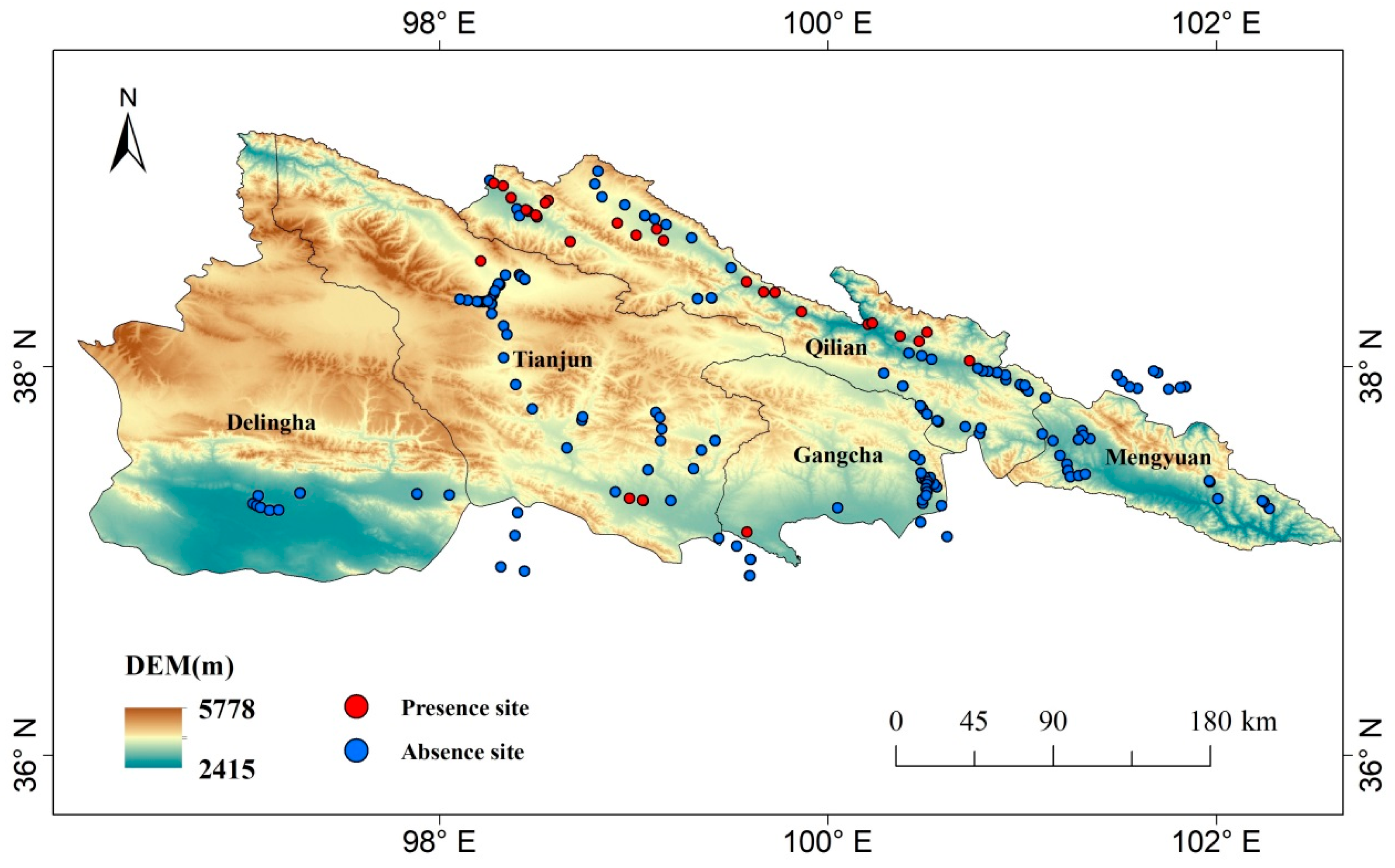
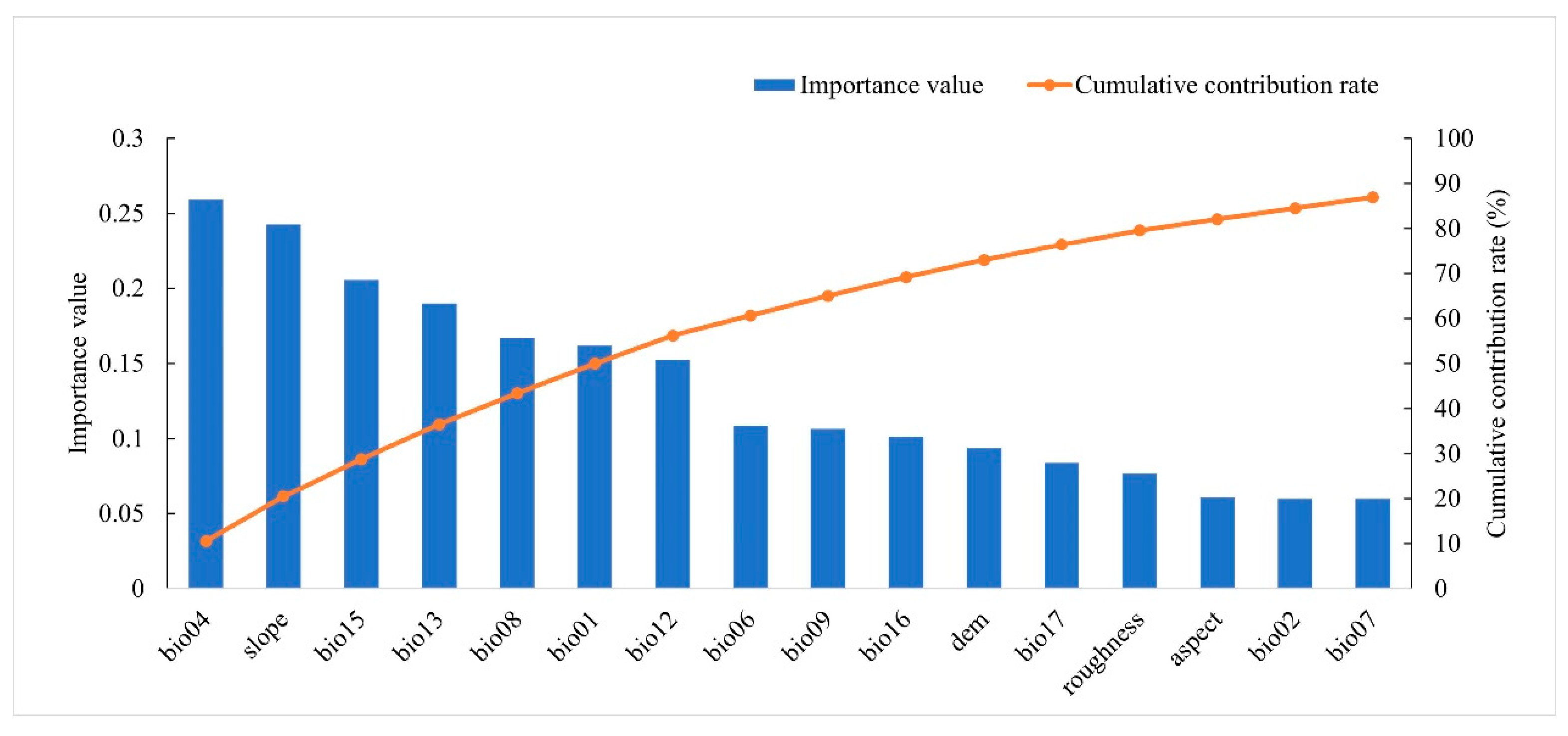
The spatial distribution of field observation for C. dubius presence and absence sites in the Qilian Mountain National Park is shown in Figure 3. Among all 298 observation sites, there was small percentage of C. dubius presence sites, accounting for 16% of total observed sites (48 observed sites). Those presence sites were mainly distributed in the central and northern areas of Qilian County, and few sample sites were distributed in the south of Gangcha and Tianjun Counties, as well as northern Tianjun County. There were 16 environmental factors, including bio4, slope, bio15, bio13, bio08, bio01, bio12, bio06, bio09, bio16, dem, bio17, roughness, aspect, bio02, and bio07, which had a cumulative contribution of more than 85% (Figure 4). Among them, bio4 (temperature seasonality), slope, and bio15 (precipitation seasonality) have higher importance than the others, with values of 0.21~0.26; they were followed in importance by bio13, bio08, bio01, bio12, bio06, bio09, and bio16, with values ranged from 0.10 to 0.19; the importance values of the rest were lower than 0.1.

3.2. Optimal Ecological Niche Model

Among all ecological niche models constructed based on the BIOMOD2 v4.2.6.2 software, the RF model exhibited the best performance, with kappa, TSS, and ROC values of 0.86, 0.90, and 0.98, respectively. They were followed in performance by GBM, FDA, GLM, MARS, and CTA models, with kappa ranging from 0.71 to 0.87, TSS ranging from 0.70 to 0.87, and ROC ranging from 0.86 to 0.97. The SRE model exhibited the lowest performance, with kappa, TSS, and ROC values of 0.36, 0.36, and 0.68, respectively (Table 2).

3.3. Spatial Distribution of C. dubius Presence Probability in the Current Situation

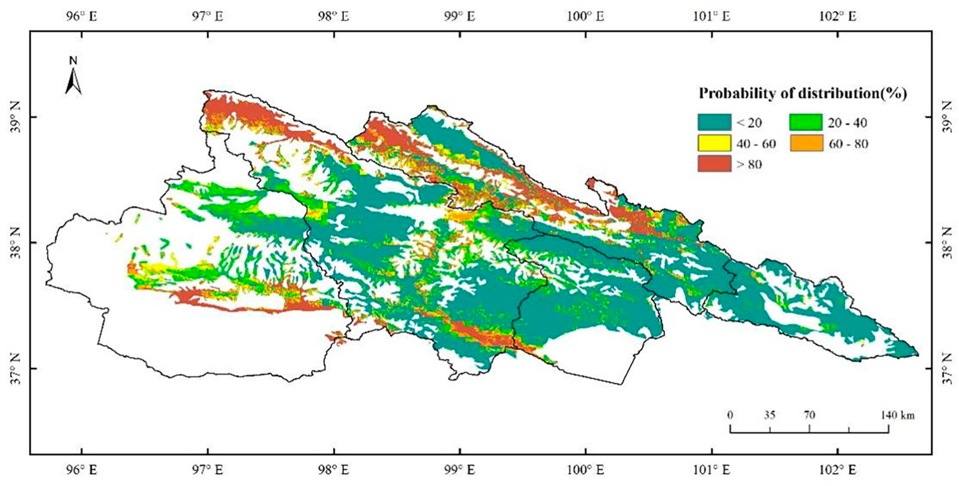
Based on the optimal ecological niche model (RF model) selected in Section 3.2, the spatial distribution of C. dubius presence probability in the current situation was inversed (Figure 5). Most of the study area exhibited a low presence probability (less than 20%), accounting for 58.45% of the total study area and mainly distributed in the center of Menyuan, Gangcha, and Tianjun Counties, and northern and southern Qilian County. They were followed in percentage by the areas with a presence probability higher than 80%, with 13.78% of the total study area, mainly distributed in the center and southwest of Qilian County, northern and southeastern Tianjun County, and the south of Delingha City. The areas with C. dubius presence probability within 20–40% (13.30% of the total study area) were mainly distributed in the center of Gangcha and Tianjun Counties, as well as most regions of Delingha City. Among all C. dubius presence probability types, the areas with a probability within 40–60% and 60–80% made up a small percentage, with 7.95% and 6.51% of the total study area, respectively. These intermediate classes were spatially scattered, occurring between areas of very low (<20%) and very high (>80%) probability.

3.4. Temporal and Spatial Dynamics Variation in C. dubius Presence Probability in Different Climate Scenarios

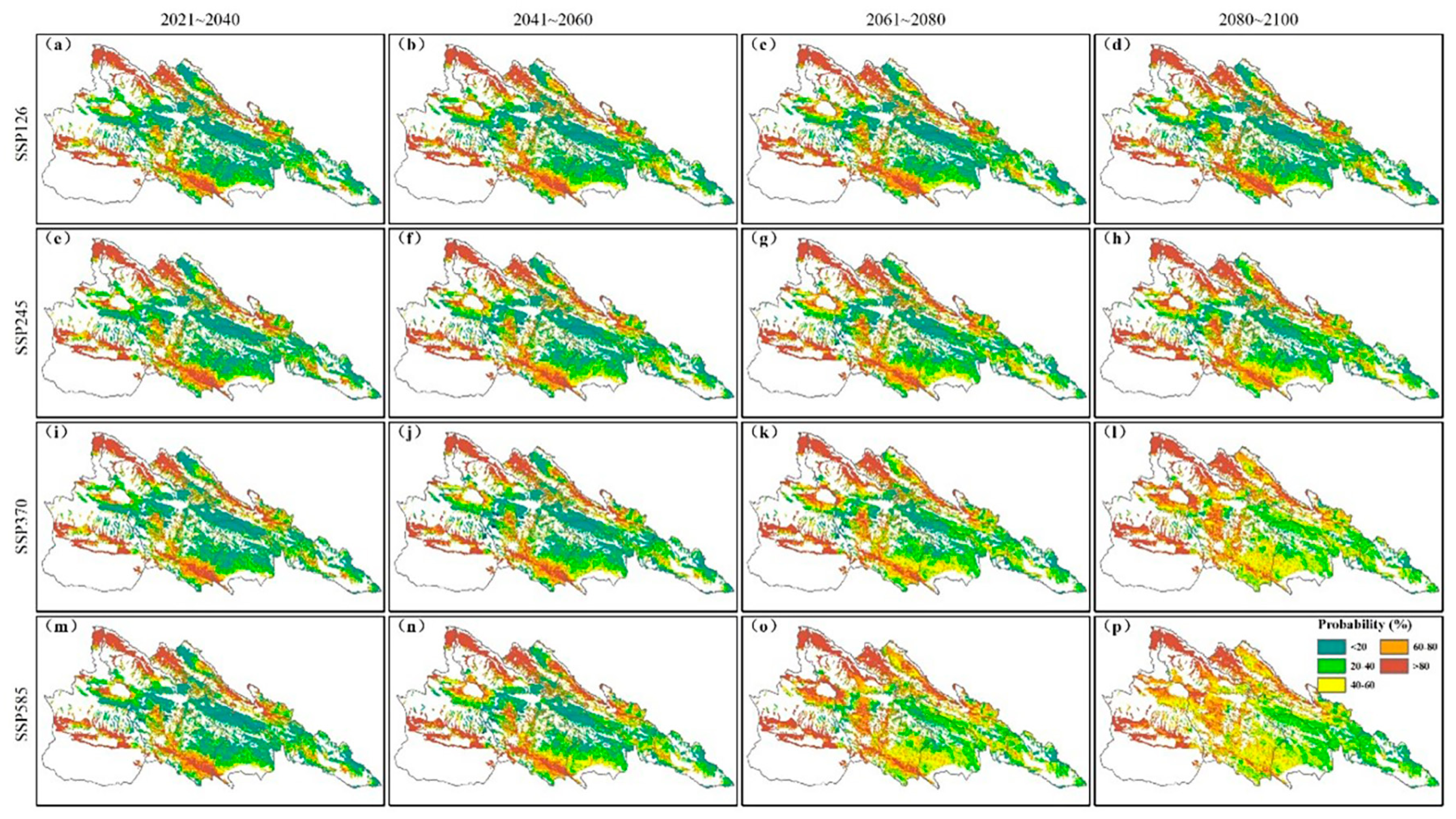
The distribution of C. dubius presence probability was calculated based on the RF and future climate dataset in four time periods (2021–2040, 2041–2060, 2061–2080, and 2081–2100) and four climate scenarios (SSPs 1–2.6, 2–4.5, 3–7.0, and 5–8.5) (Table 3 and Figure 6). In each time period and climate scenario, the area with a C. dubius presence probability of less than 20% showed a decreasing trend, and others (20% to 40%, 40% to 60%, 60% to 80%, and over 80%) presented a gradually increasing trend. Furthermore, the extent of variation in the trend increased in the order of climate scenarios SSP126, SSP245, SSP370, and SSP585, as well as in the order of time periods 2021–2040, 2041–2060, and 2061–2080. In each time period, the region of lower presence probability (less than 20%) was transformed to higher presence probability area (higher than 20%) from SSP126 to SSP245, SSP370, and SSP585 (Table 3). And the degree of transition increased from 2021–2040 to 2041–2060, 2061–2080, and 2081–2100. Among the four periods, the transition of C. dubius presence probability among SSP126, SSP245, SSP370, and SSP585 in the 2021–2040 period was the lowest, while the 2081–2100 period was the highest.
The spatial distribution of C. dubius presence probability in four time periods and four climate scenarios is shown in Figure 6. There was an increasing trend in C. dubius presence probability from northwest to southeast in each climate scenario from 2021–2040 to 2041–2060, 2061–2080, and 2081–2100 or each time period from SSP126 to SSP245, SSP370, and SSP585. In the time period of 2021–2040, the transition of C. dubius presence probability types mainly occurred in areas with a probability of less than 20% or higher than 80%. However, in the periods of 2041–2060, 2061–2080, and 2081–2100, the transition of C. dubius presence probability mainly occurred in areas with a probability of less than 20%, 40–60%, and 60–80%, respectively (Figure 6 and Table 3).

3.5. Transition in C. dubius Presence Probability Under Climate Change

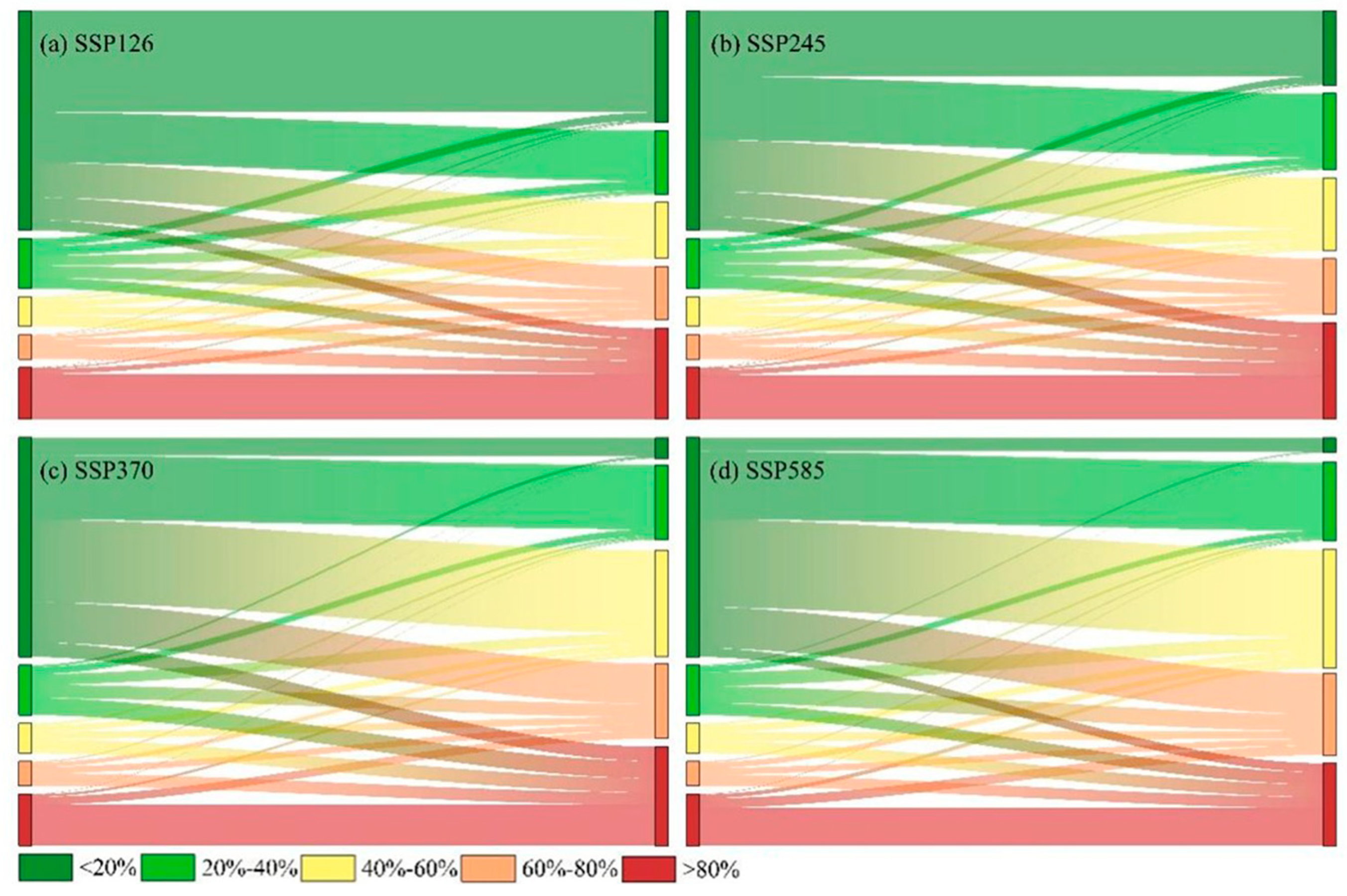
Among the four time periods, the maximum transition in C. dubius presence probability type occurred in the time period of 2081–2100. The transitions in C. dubius presence probability types between the current and future climate situation (in 2081–2100) are shown in Figure 7. The areas with a probability of less than 20% decreased in SSP126, SSP245, SSP370, and SSP585, and their proportion changed from 58.46% to 3.99%. About 93.17% of those areas transformed into the other four types. The areas of 20–40%, 40–60%, and 60–80% C. dubius presence probability types were increased by 1.56, 3.96, and 3.34 times, respectively. The areas of C. dubius presence probability higher than 80% exhibited a trend of increasing at first and then decreasing. The maximum area occurred in SSP370, with 26.34% of the total study area, which was 1.91 times the current situation. And in the SSP585 scenario, those areas decreased to 21.96%, which is 1.59 times the current situation.

4. Discussion

4.1. Distribution and Influenced Factors of C. dubius

Outbreaks of grasshoppers require particular weather, soil, and proper vegetation conditions [19]. Our study selected C. dubius as the research subject. However, C. dubius does not exist in isolation, but co-occurs with other orthopteran species, whose abundances and interactions are influenced by vegetation composition, productivity, and resource availability. Changes in these plant community attributes under climate change can alter dietary overlap and interspecific competition, potentially reshaping local assemblages and population dynamics [27,28,29]. In addition, our results showed that climate change was one of the vital factors which may lead to outbreaks of C. dubius. On the one hand, the intensification of extreme weather events may influence breeding and egg hatching of C. dubius and is conducive to their reproduction. For example, higher rainfall (more than 200 mm) provides favorable conditions for C. dubius to lay eggs (moist and fresh sandy soil) in semi-arid regions [30]. And the higher temperature (42–43 °C) can speed up the hatching period by more than two times [31]. On the other hand, these extreme weather events allowed the third generation of C. dubius to develop until they spread to a wider area. As soon as the conditions become unfavorable, C. dubius move with the wind toward other areas where conditions are more suitable for survival and breeding [32].
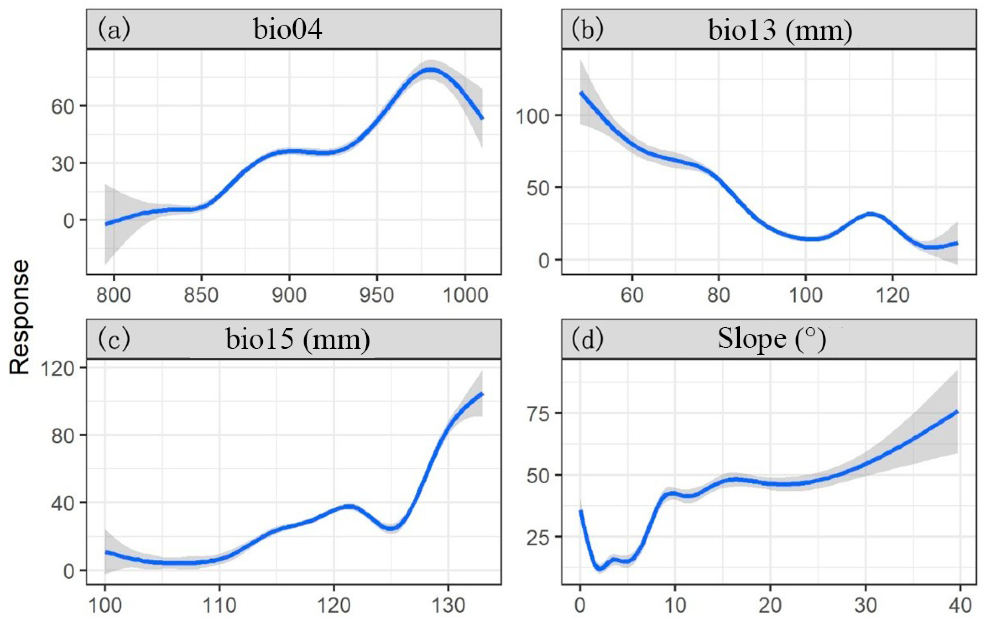
Among all environmental factors in this study, the factors with importance values of around 0.2 were the seasonal variation coefficient of temperature (bio04), the precipitation in the wettest month (bio13), the seasonal variation of precipitation (bio15), and slope (Figure 4). The response relationship between the four environmental factors and C. dubius presence probability is shown in Figure 8. Among the four environmental factors, with the gradual increase in bio04, the C. dubius presence probability presented a trend of at first increasing and then decreasing; the maximum C. dubius presence probability occurred at 985. As bio13 increased, the C. dubius presence probability showed a decreasing trend. The C. dubius presence probability tends to be 0% when the precipitation in the wettest month exceeds 120 mm. The C. dubius presence probability exhibited a fluctuating increasing trend when bio15 exceeds 110 mm. This phenomenon likely occurs because warmer conditions accelerate the developmental rate of eggs and the growth rate of nymphs, while cooler temperatures induce diapause or developmental arrest. Furthermore, increased precipitation enhances vegetation coverage and soil moisture, which in turn promotes nymphal development and aggregation [7,9]. Hence, the increase in frequency of extreme climate events, such as warming and increased rainfall, may lead to an increase in C. dubius presence probability [16,19,33]. Furthermore, our results also indicated that slope had a significant impact on the C. dubius presence probability: the C. dubius presence probability showed a decreasing trend in flat terrain areas (slope < 5°) with increasing slope. When the slope was within 5–15°, the C. dubius presence probability showed an increasing trend, while the increasing trend became weaker when the slope exceeded 15°. Our results are similar to the study of Zhu et al. (2016) [34].
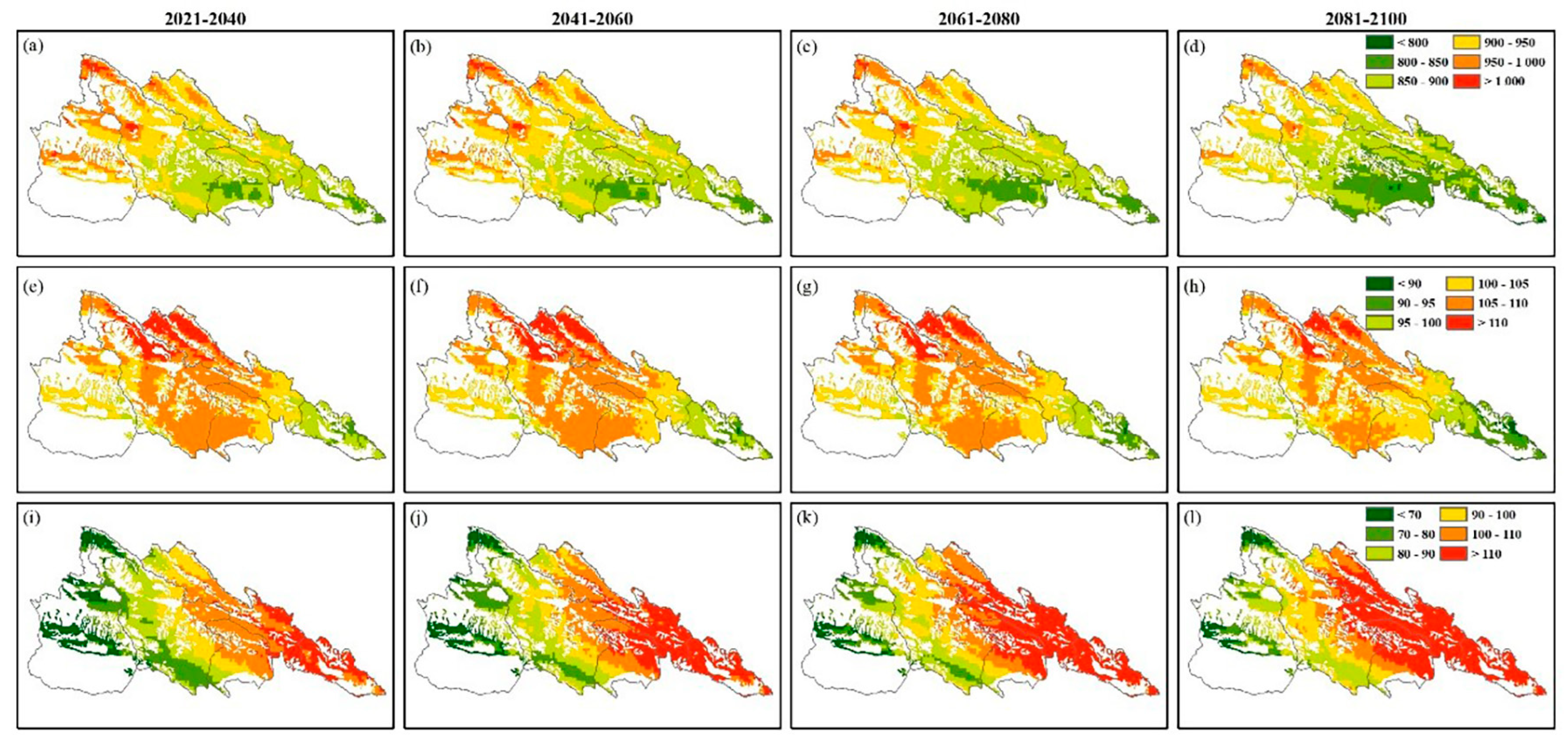
Figure 9 depicts the spatial variation of the four environmental factors in different periods and climate scenarios. The region with a bio04 value higher than 900 was primarily located in the northwest of the study area and exhibited a decreasing trend from southeast to northwest across the time periods of 2021–2040, 2041–2060, 2061–2080, and 2081–2100. Conversely, the region with a bio04 value of less than 900 showed an increasing trend from southeast to northwest. The regions with bio13 values higher than 105 mm exhibited a decreasing trend, while those with values less than 105 mm showed an increasing trend. The values of bio15 displayed an overall increasing trend from southeast to northwest. Therefore, considering the response curves of environmental factor variation in Figure 8, the C. dubius presence probability is projected to increase from northwest to southeast in future climate scenarios.

4.2. Limitations and Prospects

The study of C. dubius presence probability in the alpine grasslands of the Qilian Mountain National Park and response to climate change is crucial for assessing and customizing C. dubius hazards assessment and controlling plans in the region [35]. In this study, based on the BIOMOD ecological niche model and WorldClim climate dataset, the spatial and temporal variation in C. dubius presence probability was clarified. Our results provided a scientific reference for C. dubius damage management in the alpine grassland of the Qilian Mountains. However, this study has some limitations and shortcomings: (1) The observation data used in this study was obtained through field surveys by humans, limited by the labor, cost, and materials, and the representation of field observation is still lacking. (2) Due to the limited spatial resolution of environmental variables (about 2.5′), there are still errors and uncertainties in the simulated results of C. dubius presence probability.
The accuracy of C. dubius spatial positioning directly influences the determination of C. dubius plague prediction, evaluation, and management. Traditional field observation methods cannot easily achieve satisfactory C. dubius monitoring in vast natural pasture. Additionally, due to the small size of individual C. dubius, it is impossible to directly monitor them based on remote sensing images. Therefore, the evaluation of C. dubius occurrence locations can only be achieved by monitoring the habitats C. dubius inhabit [1,22,36].
Image processing technology has been applied in pest recognition in several studies [37,38,39,40,41], particularly in the identification of grasshoppers, which has been achieved by Mao et al. [39]. Therefore, it is possible to carry out low-altitude flights using unmanned aerial vehicles (UAVs) and manually identify the number of grasshoppers in the captured images to estimate their density [42,43]. However, most of these are case studies and lack practical application. The integration of UAV surveillance with long-term, large-scale, and repeated monitoring should be considered, and automatic identification technology should be developed in future grasshopper studies. Despite the limitations of our study, the results provide guidance for ecosystem management and grasshopper population control under future scenarios and suggest that maintaining habitat quality could help mitigate potential socio-economic impacts on local communities.

5. Conclusions

In this study, the BIOMOD2 framework was used to construct the optimal ecological niche model for C. dubius in Qilian Mountain National Park, based on the WorldClim dataset and selected environmental variables. The spatial and temporal variation in C. dubius presence probability was analyzed. The findings indicate the following: (1) Out of the 28 environmental factors considered, 16 were identified as the main influencing factors of C. dubius presence probability in alpine grasslands, including bio4, slope, bio15, bio13, bio08, bio01, bio12, bio06, bio09, bio16, dem, bio17, roughness, aspect, bio02, and bio07, with a cumulative contribution rate of over 85%. (2) Among the various ecological niche models examined, the RF model exhibited the best performance, with kappa, TSS, and ROC values of 0.86, 0.90, and 0.98, respectively. (3) In the current climate scenario, areas with higher C. dubius presence probability (above 80%) were relatively small, accounting for 13.78% of the total area, and mainly distributed in the central and southwestern regions of Qilian County, the northern and southeastern parts of Tianjun County, and the southern region of Delingha City. (4) In future climate scenarios, areas with higher C. dubius presence probability showed an increasing trend from northwest to southeast. Long-term, large-scale, fixed-point repeated aerial observations based on UAV aerial photography and grasshopper identification using machine learning algorithms will be crucial for grassland grasshopper monitoring in the future.

Supplementary Materials

The following supporting information can be downloaded at: https://www.mdpi.com/article/10.3390/agronomy15122728/s1, Figure S1: The spatial distribution of aboveground biomass (AGB) at periods of 2021–2040, and 2081–2100, under Shared Socio-economic Pathways (SSPs) 1–2.6, 2–4.5, 3–7.0and 5–8.5 on the Qilian Mountain National Park; Figure S2: Autocorrelation analysis of environmental factors; Figure S3: Cumulative contribution rates of environmental factors; Table S1: Sample data for the autocorrelation analysis of environmental factors; Table S2: Sample data of cumulative contribution rates of environmental factors; Table S3: SSP and related abbreviations with full names.

Author Contributions

Y.W.: Writing—Original Draft, Methodology, Software, Formal Analysis, Visualization, and Writing—Review and Editing; B.M.: Conceptualization, Writing—Original Draft, Software, Methodology, Supervision, Funding Acquisition, and Project Administration; H.Y.: Investigation, Writing—Review and Editing, Funding Acquisition; S.Y.: Conceptualization, Resources, Funding Acquisition, and Supervision; C.Y.: Writing—Original Draft, and Visualization; G.J.: Writing—Original Draft, and Visualization; W.X.: Writing—Original Draft, and Visualization. All authors have read and agreed to the published version of the manuscript.

Funding

This study was supported by Qinghai Province Natural Science Fund (2024-ZJ-750), 2025 Qinghai Province Fiscal Forestry and Grassland Science and Technology Promotion Demonstration Project (QLK-2025-86), and 2025 Qinghai Province Fiscal Special Fund Project for National Park (QLK-2025-71).

Data Availability Statement

The raw data supporting the conclusions of this article will be made available by the authors on request.

Acknowledgments

The authors thank the Qinghai Service and Guarantee Center of Qilian Mountain National Park and the Qinghai Province Grassland Station in Haibei Prefecture for their help in the field observation. Furthermore, we used ChatGPT v4.0 as a tool for grammar and spelling checks during the manuscript writing process.

Conflicts of Interest

The authors declare that they have no known competing financial interests or personal relationships that could have appeared to influence the work reported in this paper.

References

  1. Ciancio, A.; Mukerji, K.G. (Eds.) Integrated Management of Arthropod Pests and Insect Borne Diseases; Springer Science & Business Media: Berlin/Heidelberg, Germany, 2010; Volume 5. [Google Scholar]
  2. Krall, S. Desert Locusts in Africa: A Disaster? Disasters 1995, 19, 1–7. [Google Scholar] [CrossRef]
  3. Veran, S.; Simpson, S.J.; Sword, G.A.; Deveson, E.; Piry, S.; Hines, J.E.; Berthier, K. Modeling spatiotemporal dynamics of outbreaking species: Influence of environment and migration in a locust. Ecology 2015, 96, 737–748. [Google Scholar] [CrossRef]
  4. Hong, J.; Du, G.; Wang, G. The occurring and control situation of grasshopper in the grassland of China (review). Acta Agrestia Sin. 2014, 22, 929–934. [Google Scholar]
  5. Le Gall, M.; Overson, R.; Cease, A. Corrigendum: A global review on locusts (Orthoptera: Acrididae) and their interactions with livestock grazing practices. Front. Ecol. Evol. 2023, 11, 1154640. [Google Scholar] [CrossRef]
  6. Zhang, X.; Huang, W.; Ye, H.; Lu, L. Study on the identification of habitat suitability areas for the dominant locust species Dasyhippus barbipes in Inner Mongolia. Remote Sens. 2023, 15, 1718. [Google Scholar] [CrossRef]
  7. Wu, T.; Hao, S.; Kang, L. Effects of soil temperature and moisture on the development and survival of grasshopper eggs in inner mongolian grasslands. Front. Ecol. Evol. 2021, 9, 727911. [Google Scholar] [CrossRef]
  8. Mitra, B.; Gayen, A.; Haque, S.M.; Das, A. Influence of climate on desert locust (Schistocerca gregaria Forskål, 1775) Plague and migration prediction in tropics. Sci. Rep. 2024, 14, 24270. [Google Scholar] [CrossRef]
  9. Symmons, P.M.; Cressman, K. Desert Locust Guidelines: Biology and Behaviour; FAO: Rome, Italy, 2001; Volume 42. [Google Scholar]
  10. Chen, Y.; Han, M.; Yuan, X.; Hou, Y.; Qin, W.; Zhou, H.; Zhao, X.; Klein, J.A.; Zhu, B. Warming has a minor effect on surface soil organic carbon in alpine meadow ecosystems on the Qinghai–Tibetan Plateau. Glob. Change Biol. 2022, 28, 1618–1629. [Google Scholar] [CrossRef] [PubMed]
  11. Miehe, G.; Schleuss, P.-M.; Seeber, E.; Babel, W.; Biermann, T.; Braendle, M.; Chen, F.; Coners, H.; Foken, T.; Gerken, T.; et al. The Kobresia pygmaea ecosystem of the Tibetan highlands—Origin, functioning and degradation of the world’s largest pastoral alpine ecosystem: Kobresia pastures of Tibet. Sci. Total Environ. 2019, 648, 754–771. [Google Scholar] [CrossRef] [PubMed]
  12. Ran, Q.; Hao, Y.; Xia, A.; Liu, W.; Hu, R.; Cui, X.; Xue, K.; Song, X.; Xu, C.; Ding, B.; et al. Quantitative assessment of the impact of physical and anthropogenic factors on vegetation spatial-temporal variation in Northern Tibet. Remote Sens. 2019, 11, 1183. [Google Scholar] [CrossRef]
  13. Zhan, T.; Zhao, W.; Feng, S.; Hua, T. Plant community traits respond to grazing exclusion duration in alpine meadow and alpine steppe on the Tibetan plateau. Front. Plant Sci. 2022, 13, 863246. [Google Scholar] [CrossRef]
  14. Zavaleta, E.S.; Shaw, M.R.; Chiariello, N.R.; Mooney, H.A.; Field, C.B. Additive effects of simulated climate changes, elevated CO2, and nitrogen deposition on grassland diversity. Proc. Natl. Acad. Sci. USA 2003, 100, 7650–7654. [Google Scholar] [CrossRef]
  15. Zhao, J.; Li, X.; Li, R.; Tian, L.; Zhang, T. Effect of grazing exclusion on ecosystem respiration among three different alpine grasslands on the central Tibetan Plateau. Ecol. Eng. 2016, 94, 599–607. [Google Scholar] [CrossRef]
  16. Ni, S. Remote Sensing Monitoring and Prediction of Grasshopper in Qinghai Lake; Shanghai Science and Technology Press: Shanghai, China, 2002. [Google Scholar]
  17. Zhang, L.; Lecoq, M.; Latchininsky, A.; Hunter, D. Locust and grasshopper management. Annu. Rev. Entomol. 2019, 64, 15–34. [Google Scholar] [CrossRef]
  18. Laws, A.N.; Prather, C.M.; Branson, D.H.; Pennings, S.C. Effects of grasshoppers on prairies: Herbivore composition matters more than richness in three grassland ecosystems. J. Anim. Ecol. 2018, 87, 1727–1737. [Google Scholar] [CrossRef]
  19. Shuang, L.I.; Ullah, H.; Zhang, Z. IPM-Biological and integrated management of desert locust. J. Integr. Agric. 2022, 21, 3467–3487. [Google Scholar]
  20. Li, Z.; Yuan, R.; Feng, Q.; Zhang, B.; Lv, Y.; Li, Y.; Wei, W.; Chen, W.; Ning, T.; Gui, J.; et al. Climate background, relative rate, and runoff effect of multiphase water transformation in Qilian Mountains, the third pole region. Sci. Total Environ. 2019, 663, 315–328. [Google Scholar] [CrossRef]
  21. Xue, J.; Li, Z.; Feng, Q.; Li, Z.; Gui, J.; Li, Y. Ecological conservation pattern based on ecosystem services in the Qilian Mountains, northwest China. Environ. Dev. 2023, 46, 100834. [Google Scholar] [CrossRef]
  22. Lv, Y.Y.; Yu, H.Y.; Chen, W.; Li, M.; Yi, S.H.; Meng, B.P. Predicting inhabitable areas for locust based on field observation and multi-environmental factors in alpine grassland—A case study in the Qilian Mountain National Park, China. Front. Ecol. Evol. 2023, 11, 1149952. [Google Scholar] [CrossRef]
  23. Yang, L.; Feng, Q.; Adamowski, J.F.; Alizadeh, M.R.; Yin, Z.; Wen, X.; Zhu, M. The role of climate change and vegetation greening on the variation of terrestrial evapotranspiration in northwest China’s Qilian Mountains. Sci. Total Environ. 2021, 759, 143532. [Google Scholar] [CrossRef]
  24. Guo, Y.; Li, X.; Zhao, Z.; Nawaz, Z. Predicting the impacts of climate change, soils and vegetation types on the geographic distribution of Polyporus umbellatus in China. Sci. Total Environ. 2019, 648, 1–11. [Google Scholar] [CrossRef] [PubMed]
  25. Zhang, H.; Tang, Z.; Wang, B.; Kan, H.; Sun, Y.; Qin, Y.; Meng, B.; Li, M.; Chen, J.; Lv, Y.; et al. A 250 m annual alpine grassland AGB dataset over the Qinghai–Tibet Plateau (2000–2019) in China based on in situ measurements, UAV photos, and MODIS data. Earth Syst. Sci. Data 2023, 15, 821–846. [Google Scholar] [CrossRef]
  26. Fawcett, T. An introduction to ROC analysis. Pattern Recognit. Lett. 2006, 27, 861–874. [Google Scholar] [CrossRef]
  27. Branson, D.H.; Sergeev, M. Relationships between Plant Diversity and Grasshopper Diversity and Abundance in the Little Missouri National Grassland. Psyche-J. Entomol. 2010, 2011, 37. [Google Scholar] [CrossRef]
  28. Cease, A.J.; Elser, J.J.; Fenichel, E.P.; Hadrich, J.C.; Harrison, J.F.; Robinson, B.E. Living with locusts: Connecting soil nitrogen, locust outbreaks, livelihoods, and livestock markets. Bioscience 2015, 65, 551–558. [Google Scholar] [CrossRef]
  29. Joern, A. Disturbance by fire frequency and bison grazing modulate grasshopper assemblages in tallgrass prairie. Ecology 2005, 86, 861–873. [Google Scholar] [CrossRef]
  30. Uvarov, B. Grasshoppers and locusts. In A Handbook of General Acridology, Behaviour, Ecology, Biogeography, Population Dynamics; Centre for Overseas Pest Research: London, UK, 1997; Volume 2, pp. 1–613. [Google Scholar]
  31. Nishide, Y.; Suzuki, T.; Tanaka, S. The hatching time of Locusta migratoria under outdoor conditions: Role of temperature and adaptive significance. Physiol. Entomol. 2017, 42, 146–155. [Google Scholar] [CrossRef]
  32. Cressman, K. Current methods of desert locust forecasting at FAO. EPPO Bull. 1996, 26, 577–585. [Google Scholar] [CrossRef]
  33. Zhang, Z.; Li, D. A possible relationship between outbreaks of the oriental migratory locust (Locusta migratoria manilensis Meyen) in China and the El Niño episodes. Ecol. Res. 1999, 14, 267–270. [Google Scholar] [CrossRef]
  34. Zhu, M.M.; Zhang, R.; Zhang, Z.H. The responses of grasshoppers and their natural enemies to soil humidity and slope in Mahuang Mountain. Ningxia 2016, 43, 369–376. [Google Scholar]
  35. Ji, R.; Xie, B.-Y.; Li, D.-M.; Li, Z.; Zhang, X. Use of MODIS data to monitor the oriental migratory locust plague. Agric. Ecosyst. Environ. 2004, 104, 615–620. [Google Scholar] [CrossRef]
  36. Dong, Y.; Zhao, L.; Huang, W. Monitoring of Desert Locust in Africa and Asia; Springer: Berlin/Heidelberg, Germany, 2023. [Google Scholar]
  37. Hamuda, E.; Glavin, M.; Jones, E. A survey of image processing techniques for plant extraction and segmentation in the field. Comput. Electron. Agric. 2016, 125, 184–199. [Google Scholar] [CrossRef]
  38. Hamuda, E.; Mc Ginley, B.; Glavin, M.; Jones, E. Improved image processing-based crop detection using Kalman filtering and the Hungarian algorithm. Comput. Electron. Agric. 2018, 148, 37–44. [Google Scholar] [CrossRef]
  39. Mao, W.; Zheng, Y.; Zhang, Y.; Yuan, Y.; Zhang, X. Grasshopper detection method based on machine vision. Agric. Eng. 2008, 24, 155–158. [Google Scholar]
  40. Hansen, O.L.P.; Svenning, J.; Olsen, K.; Dupont, S.; Garner, B.H.; Iosifidis, A.; Price, B.W.; Høye, T.T. Species-level image classification with convolutional neural network enables insect identification from habitus images. Ecol. Evol. 2020, 10, 737–747. [Google Scholar] [CrossRef]
  41. Ikemoto, N.; Terada, K.; Takashina, Y.; Nakano, A. High-precision Classification of Small Insects with Similar Color and Shape Using Image Processing. Electron. Commun. Jpn. 2017, 100, 73–82. [Google Scholar] [CrossRef]
  42. Hunt, E.R., Jr.; Rondon, S.I. Detection of potato beetle damage using remote sensing from small unmanned aircraft systems. J. Appl. Remote Sens. 2017, 11, 026013. [Google Scholar] [CrossRef]
  43. Yuba, N.; Kawamura, K.; Yasuda, T.; Lim, J.; Yoshitoshi, R.; Kurokawa, Y.; Maeda, T. Counting of Pennisetum alopecuroides at heading stage in a grazed pasture using images from an unmanned aerial vehicle. Grassl. Sci. 2020, 66, 285–292. [Google Scholar] [CrossRef]
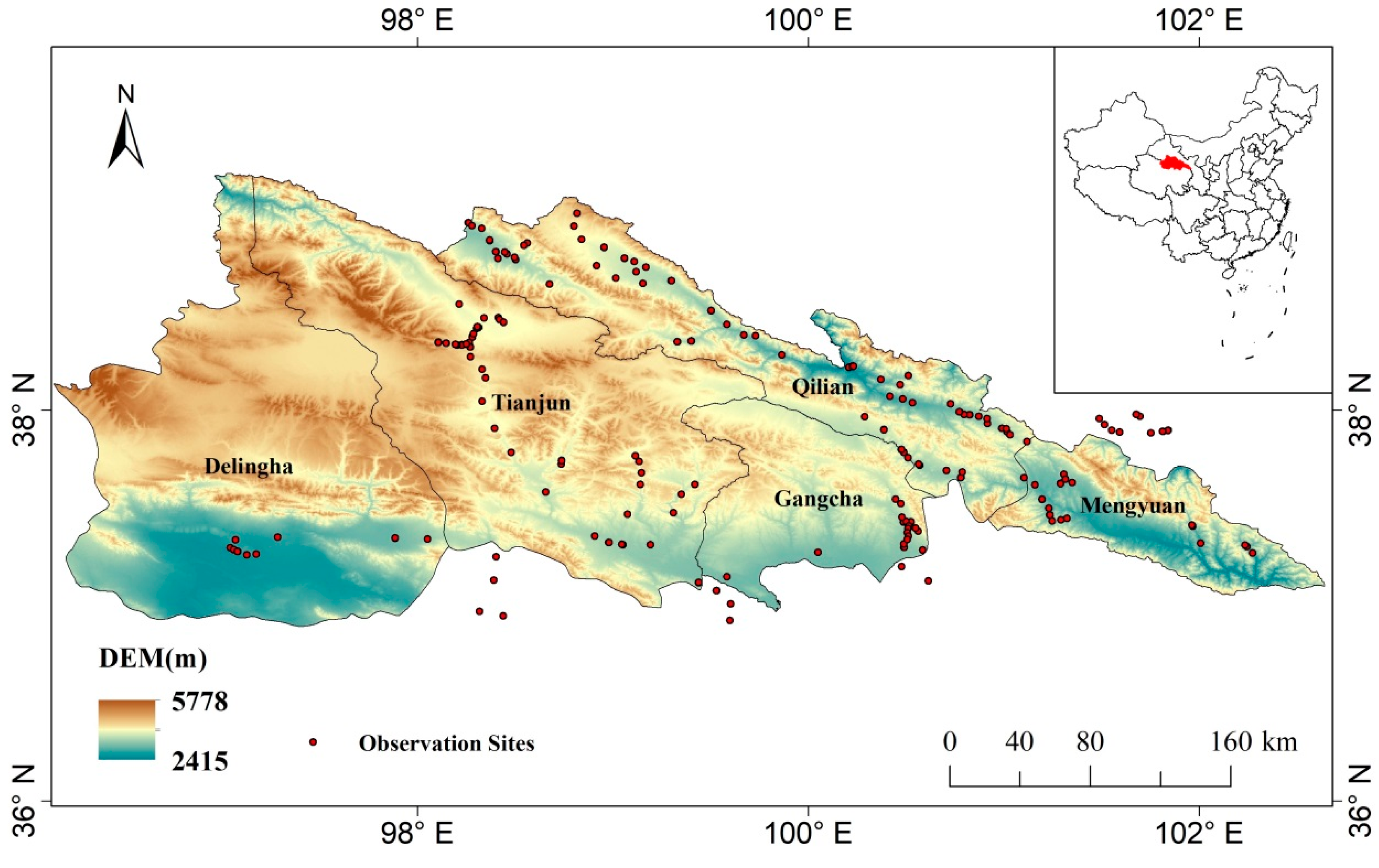
Figure 1. Location and observation of study area. DEM refers to the digital elevation model.
Agronomy 15 02728 g001
Figure 2. Field observation. (a) Collection by butterfly net; (b) collection by enclosure method (50 cm × 50 cm × 50 cm).
Agronomy 15 02728 g002
Figure 3. Spatial distribution of C. dubius presence sites in Qilian Mountain National Park.
Agronomy 15 02728 g003
Figure 4. Importance value and cumulative contribution rate of 16 environmental factors, bio4, slope, bio15, bio13, bio08, bio01, bio12, bio06, bio09, bio16, dem, bio17, roughness, aspect, bio02, and bio07, representing temperature seasonality, slope, precipitation seasonality, precipitation of the wettest month, mean temperature of the wettest quarter, annual mean temperature, annual precipitation, min temperature of the coldest month, mean temperature of the driest quarter, precipitation of the wettest quarter, digital elevation model, precipitation of the driest quarter, roughness, aspect, mean diurnal range of temperature, and temperature annual range, respectively.
Agronomy 15 02728 g004
Figure 5. The spatial distribution of C. dubius presence probability in the current situation.
Agronomy 15 02728 g005
Figure 6. Spatial and time variation in C. dubius presence probability under climate change. (ad), (eh), (il), and (mp) represent the distribution in the climate scenario SSP126, SSP245, SSP370, and SSP585, respectively.
Agronomy 15 02728 g006
Figure 7. Spatial transitions of presence probability type in different climate scenarios between the current and 2081–2100 period. (ad) represent the climate scenarios SSP126, SSP245, SSP370, and SSP585, respectively.
Agronomy 15 02728 g007
Figure 8. Response curves for presence probability and environmental variables. (ad) represent bio04, bio13, bio15, and slope.
Agronomy 15 02728 g008
Figure 9. Spatial-temporal variation of three environmental factors from 2021–2040 to 2041–2060, 2061–2080, and 2081–2100. (ad), (eh), and (il) refers to bio4, bio13, and bio15, respectively.
Agronomy 15 02728 g009
Table 1. Filtered environment variables.
Environment VariablesCodeVariable
Climate variablesbio01Annual Mean Temperature
bio02Mean Diurnal Range
bio04Temperature Seasonality
bio06Min Temperature of Coldest Month
bio07Temperature Annual Range
bio08Mean Temperature of Wettest Quarter
bio09Mean Temperature of Driest Quarter
bio12Annual Precipitation
bio13Precipitation of Wettest Month
bio15Precipitation Seasonality
bio16Precipitation of Wettest Quarter
bio17Precipitation of Driest Quarter
Topographic variablesdemDigital Elevation Model
slopSlope
aspeAspect
Other variablesroughnessSurface Roughness
Table 2. Accuracy evaluation of kappa, TSS, and ROC for each model.
ModelAccuracy
KappaTSSROC
GLM0.780.830.92
GBM0.840.870.97
CTA0.710.700.86
SRE0.360.360.68
FDA0.870.860.93
MARS0.780.800.90
RF0.860.900.98
Table 3. The area proportion of C. dubius presence probability in different climate scenarios and time periods.
PeriodProbability (%)Proportion of Area (%)
SSP126SSP245SSP370SSP585
2021–2040<200.350.320.340.33
20–400.180.180.180.18
40–600.140.140.140.14
60–800.120.130.130.13
>800.200.220.210.22
2041–2060<200.310.300.300.24
20–400.170.180.190.19
40–600.150.160.160.17
60–800.140.140.130.15
>800.230.220.220.25
2061–2080<200.310.250.180.08
20–400.170.190.220.19
40–600.150.170.210.25
60–800.140.150.150.19
>800.230.240.240.29
2081–2100<200.300.200.060.04
20–400.170.200.200.21
40–600.150.190.280.31
60–800.140.150.200.22
>800.240.260.260.22
Disclaimer/Publisher’s Note: The statements, opinions and data contained in all publications are solely those of the individual author(s) and contributor(s) and not of MDPI and/or the editor(s). MDPI and/or the editor(s) disclaim responsibility for any injury to people or property resulting from any ideas, methods, instructions or products referred to in the content.