Article

Detecting Abandoned Cropland in Monsoon-Influenced Regions Using HLS Imagery and Interpretable Machine Learning

1
Department of Forest Resources, Kookmin University, 77 Jeongneung-ro, Seongbuk-gu, Seoul 02707, Republic of Korea
2
Department of Forest, Environment, and Systems, Kookmin University, 77 Jeongneung-ro, Seongbuk-gu, Seoul 02707, Republic of Korea
3
Forest Carbon Graduate School, Kookmin University, 77 Jeongneung-ro, Seongbuk-gu, Seoul 02707, Republic of Korea
*
Author to whom correspondence should be addressed.
Agronomy 2025, 15(12), 2702; https://doi.org/10.3390/agronomy15122702
Submission received: 29 October 2025 / Revised: 18 November 2025 / Accepted: 20 November 2025 / Published: 24 November 2025

Abstract

Abandoned cropland has been expanding due to complex socio-economic factors such as urbanization, demographic shifts, and declining agricultural profitability. As abandoned cropland simultaneously brings ecological, environmental, and social risks and benefits, quantitative monitoring is essential to assess its overall impact. Satellite image-based spatial data are suitable for identifying spectral characteristics related to crop phenology, and recent research has advanced in detecting large-scale abandoned cropland through changes in time-series spectral characteristics. However, frequent cloud covers and highly fragmented croplands, which vary across regions and climatic conditions, still pose significant challenges for satellite-based detection. This study combined Harmonized Landsat and Sentinel-2 (HLS) imagery, offering high temporal (2–3 days) and spatial (30 m) resolution, with the eXtreme Gradient Boosting (XGBoost) algorithm to capture seasonal spectral variations among rice paddy, upland fields, and abandoned croplands. An XGBoost model with a Balanced Bagging Classifier (BBC) was used to mitigate class imbalance. The model achieved an accuracy of 0.84, C o h e n s   k a p p a 0.71, and F 2   s c o r e 0.84. SHapley Additive exPlanations (SHAP) analysis identified major features such as NIR (May–June), SWIR2 (January), MCARI (September), and BSI (January–April), reflecting phenological differences among cropland types. Overall, this study establishes a robust framework for large-scale cropland monitoring that can be adapted to different regional and climatic settings.

1. Introduction

Abandoned cropland represents a land-use transition driven by structural changes across socioeconomic and environmental systems. It refers to previously cultivated cropland that has remained out of production for a sustained period, as determined by criteria such as the continuous cessation of cultivation, discontinuation of agricultural management, and recovery of natural vegetation [1,2]. The drivers of cropland abandonment include socioeconomic factors, such as rural population decline, population aging, and decreasing agricultural profitability, as well as environmental constraints like steep topography, high elevation, and poor soil fertility [3,4,5]. Due to these interacting factors, abandoned cropland has been rapidly expanding not only in developed regions such as Europe and North America, but also increasingly in developing areas including China and Latin America [1,6,7].
Abandoned cropland has both positive and negative environmental and socioeconomic implications. On the positive side, unmanaged cropland can undergo secondary ecological succession, leading to vegetation recovery and long-term enhancement of ecosystem services such as increased carbon sequestration, reduced soil erosion, and improved soil condition [8,9,10]. However, the rapid spread of invasive species and weeds into adjacent croplands due to the lack of active management can directly suppress farming activities and increase control costs [11], creating immediate negative impacts on surrounding agricultural areas. From a broader perspective, cropland abandonment reduces regional agricultural productivity and weakens the agricultural resource base [12]. This poses structural risks to overall agricultural self-sufficiency, ultimately affecting food security and the sustainable use and management of farmland [5,13]. Moreover, the loss of open agricultural areas reduces habitats for species adapted to cropland ecosystems, while the disappearance of traditional farming landscapes diminishes visual aesthetics and erodes the cultural and social values of rural communities [12,14,15]. Cropland abandonment is a complex process involving both ecological and socioeconomic dimensions and therefore requires systematic and continuous monitoring.
Identifying the spatio-temporal distribution of abandoned cropland is essential for understanding its expansion and developing effective, well-organized management strategies. Numerous studies have applied remote sensing-based approaches for the detection of abandoned cropland, with phenology-based methods being among the most widely used [1,16,17,18,19]. Since abandoned cropland retains vegetation and spectral properties similar to cultivated fields even after farming ceases, analyzing crop growth cycles and seasonal variation patterns is crucial for distinguishing it from active cropland. Given these complex phenological patterns, machine-learning techniques have been increasingly employed to model such patterns systematically. For instance, Wuyun et al. [20] analyzed crop-specific key growth stages in Inner Mongolia using Sentinel imagery and classified cultivated versus abandoned fields based on vegetation index characteristics using a Random Forest model. Similarly, Hong et al. [21] combine Random Forest combined with LandTrendr, a time-series change detection algorithm, using Landsat imagery to identify areas converted from cropland to grassland or other land uses. Yoon et al. [22] applied harmonic analysis to Sentinel-2 NDVI, NDWI, and SAVI time-series data to extract phenological characteristics of different land-use types and subsequently used an SVM classifier to detect abandoned cropland. Overall, previous studies have conducted large-scale regional time-series analysis utilizing medium-resolution satellite imagery from a single source, either Landsat or Sentinel. Moreover, discussions on systematic learning strategies for addressing class imbalance and on rigorous analytical procedures for model interpretability have been relatively limited.
Conventional phenology-based remote sensing approaches are designed under the assumption of access to high-quality time-series observations, and their detection accuracy declines substantially when such conditions are not met [23,24]. The East Asian monsoon is a large-scale seasonal circulation system characterized by a marked reversal of prevailing wind directions between summer and winter, resulting in pronounced seasonal contrasts in temperature and precipitation. In regions such as the Korean Peninsula, which is surrounded by seas on three sides, abundant moisture is transported from adjacent oceans during the summer monsoon, often leading to heavy rainfall events and concentrated precipitation. These meteorological conditions substantially increase cloud cover during the crop growing season, making it difficult to obtain stable optical satellite time-series observations. However, previous studies have been developed under the assumption of large-scale agricultural fields and stable weather conditions, limiting their applicability to South Korea’s agricultural environment, which is characterized by frequent cloud cover and small, highly fragmented field structures. For time-series analyses used in abandoned cropland detection, variations in regional growth conditions, climatic patterns, and soil characteristics hinder the transferability and generalization of model signatures [25]. To overcome these challenges, an explainable artificial intelligence (XAI)-based approach is required to provide a comprehensive understanding of not only vegetation index dynamics, but also the broader cropland environment, including insights into agricultural practices and underlying ecological status. In this context, time-series satellite imagery with short revisit intervals and sufficient spatial resolution is indispensable. Since abandoned cropland datasets inherently exhibit class imbalance, appropriate strategies should be implemented to ensure stable model performance.
Addressing these technical and environmental limitations aligns with South Korea’s recently revised Farmland Act, which has strengthened the management of abandoned cropland, further underscoring the need for satellite-based precision detection systems that can complement field surveys. This study aims to overcome the limitations of spatio-temporal resolution and the lack of model transferability across regions by developing a region-specific abandoned cropland detection. The model utilizes time-series spectral characteristics of high-temporal-resolution satellite imagery. The specific objectives of this study are as follows: (1) Construct a training dataset for paddy fields, upland cropland, and abandoned cropland by integrating Harmonized Landsat and Sentinel-2 (HLS) time-series imagery with field survey data, and develop a region-tailored detection model suited to South Korea’s agricultural environment. (2) Apply a learning strategy that mitigates class imbalance among cropland types to reduce data bias and improve model accuracy and stability. (3) Identify key temporal and spectral variables that distinguish abandoned cropland from paddy and upland fields through interpretable model analysis, and clarify their contribution directions and detection mechanisms.

2. Materials and Methods

2.1. Study Site

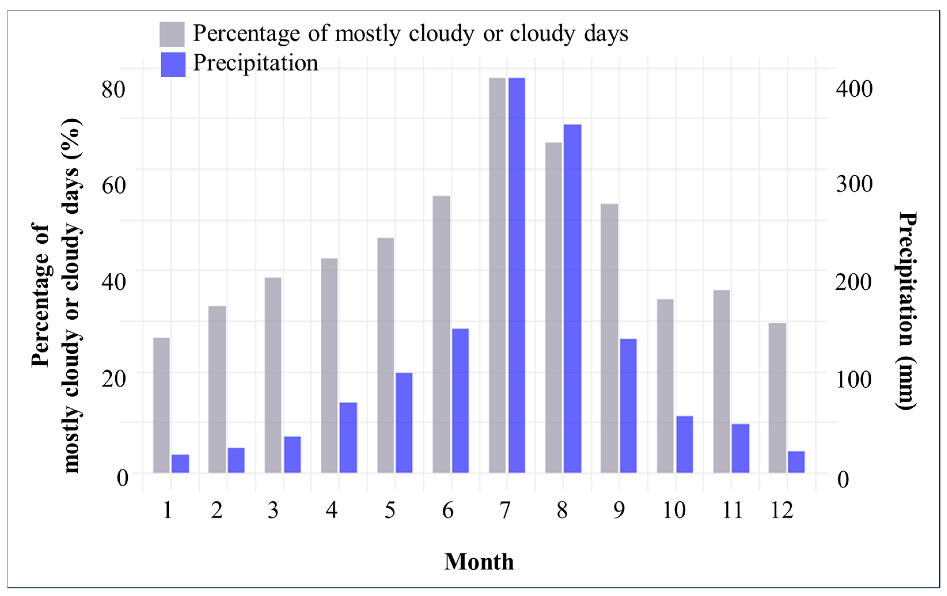
The study site, Gyeonggi-do Province in South Korea, lies within a highly urbanized metropolitan region that is under intense development pressure and a significant risk of cropland abandonment (Figure 1). According to the Köppen–Geiger climate classification, Gyeonggi-do Province falls under the monsoon-influenced hot-summer humid continental climate (Dwa) [26]. The average annual precipitation of the study area was approximately 1438 mm during 1998–2024, with cloudy or mostly cloudy conditions on 44.7% of days, most of which occurred during the summer monsoon season (Figure 2). The total cultivated area is 137,581 ha, and rice paddies cover 69,905 ha, while soybeans, perilla, and dried red peppers are also widely grown [27]. Spatial heterogeneity of cultivated land and growth differences based on latitude complicate the identification of abandoned cropland in remote sensing [28]. Furthermore, Smallholder farms account for over 37% of all agricultural production in Gyeonggi-do Province, and diverse crops are cultivated across its administrative districts [27]. To ensure consistency in analysis, this study restricted its spatial range to Namyangju-si, Dongducheon-si, Uijeongbu-si, Yangju-si, and Pocheon-si within Gyeonggi-do Province, which share similar crop production types and are spatially adjacent (Table 1).

2.2. Overall Workflow

This study aimed to develop a machine learning model for identifying abandoned cropland using time-series analysis of satellite imagery. The analysis consisted of the following four steps: (1) Satellite imagery was acquired as input features, and reference labels were established through field surveys, cadastral maps, and land cover maps. Features representing the characteristics and temporal patterns of each cropland type were extracted and subsequently selected based on multiple time-series satellite bands. (2) The Boruta algorithm was applied to identify the optimal explanatory variables for abandoned cropland detection, allowing the selection of key variables that contributed most to model performance. (3) Finally, an eXtreme Gradient Boosting (XGBoost) model with a Balanced Bagging Classifier (BBC) was developed using the selected key variables. (4) The SHapley Additive exPlanations (SHAP) analysis was then conducted to quantify the contribution of each variable and to identify the primary spectral characteristics and temporal response patterns distinguishing abandoned cropland from rice paddy and upland field. The overall data processing and analysis workflow is illustrated in Figure 3.

2.3. Data Collection: Field Survey and Satellite Imagery

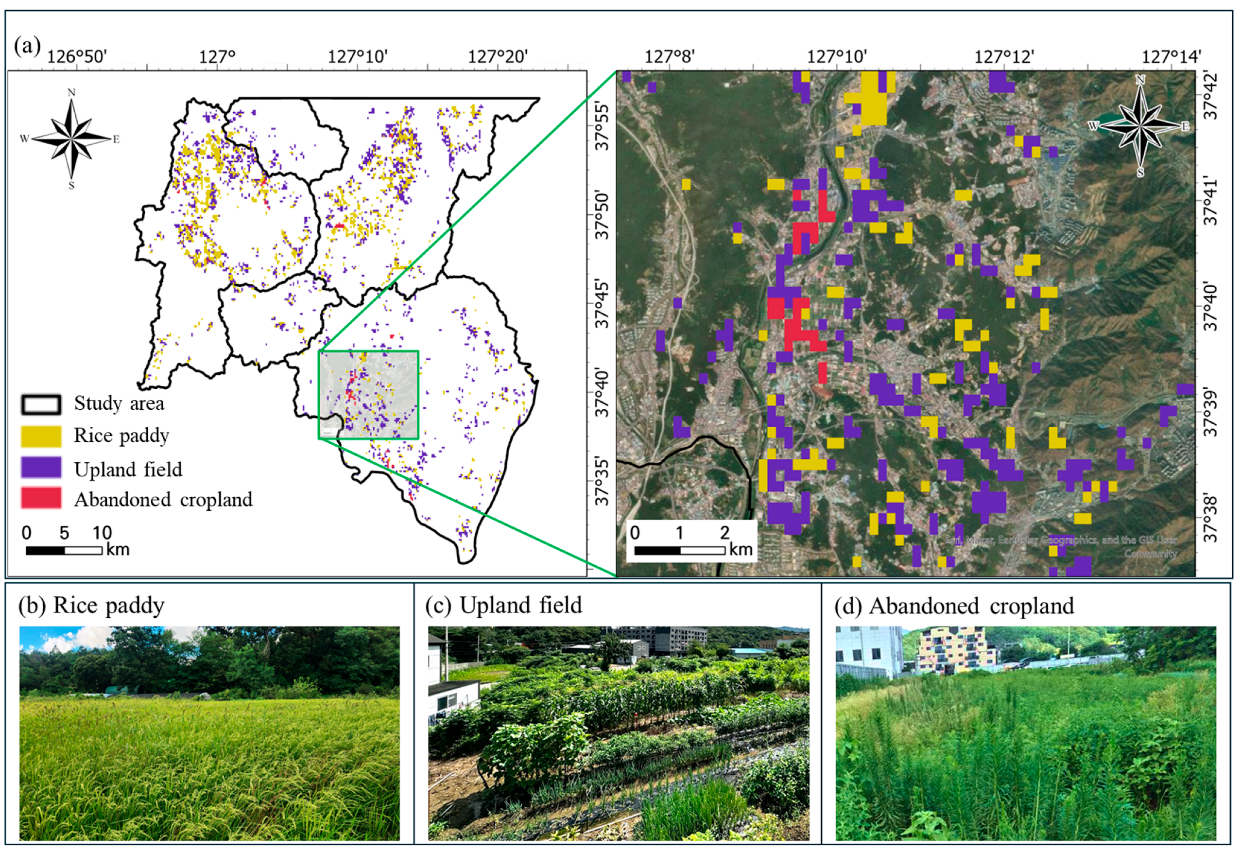
This study constructed an integrated dataset for cropland within the study area by combining the cadastral map [30], the land cover map [31], satellite imagery, and field survey data. This comprehensive dataset was used to train and validate the abandoned cropland detection model (Figure 4). To identify abandoned cropland, we focused on areas classified as cropland on both cadastral maps and land cover maps. During preprocessing, areas smaller than 1 ha or regions likely to be affected by pixel contamination, such as roads or mixed structures including plastic greenhouses, were excluded. After additional label corrections, reference data for rice paddy and upland fields were constructed. Since no public data are available for abandoned cropland, ground-truth data were collected through a 2025 field survey, resulting in 677 samples covering approximately 60.9 ha. The collected abandoned cropland samples were derived from approximately 24% rice paddies and 76% upland fields, and their slopes ranged from 0° to 21°, indicating that the samples cover a wide range of terrain conditions.
In monsoon-influenced regions such as South Korea, vegetation phenology exhibits pronounced seasonal variability throughout the year. Detecting abandoned cropland primarily depends on capturing temporal variations in vegetation phenology that distinguish it from active cultivated fields, which requires satellite imagery with high temporal resolution. Therefore, monthly 30 m spatial resolution spectral imagery was constructed from January to September 2025 using HLS, which maintain 30 m spatial resolution while improving temporal resolution, and Sentinel-1 C-band Synthetic Aperture Radar (SAR) Ground Range Detected (GRD) data, which enable continuous observation regardless of weather conditions. However, due to decreased image quality caused by snow cover in January–February and heavy rainfall in July–August, each period was grouped into a single representative month (January and August) to construct the time series.
HLS, developed by NASA, integrates surface reflectance data acquired from the Landsat-8/9 Operational Land Imager (OLI), with an approximately 8-day temporal resolution, and the Sentinel-2A/B Multi-Spectral Instrument (MSI), with an approximately 5-day temporal resolution, thereby enhancing the temporal resolution to 2–3 days [32]. To ensure consistent spectral characteristics between the two sensors, HLS performs a series of procedures including radiometric and geometric adjustments, atmospheric correction, cloud and cloud-shadow masking, and Bidirectional Reflectance Distribution Function (BRDF) normalization. Notably, it applies a bandpass adjustment algorithm that calibrates Sentinel-2 reflectance to the Landsat standard. Ultimately, HLS generates L30 (Landsat-based) and S30 (Sentinel-based) products. This study utilized both products to construct the red, green, blue, near-infrared (NIR), shortwave-infrared 1 (SWIR1), and shortwave-infrared 2 (SWIR2) bands. Additionally, the Red Edge 1 band, available only in the S30 product, was included. Because of its low temporal resolution, only images from April and September with minimal cloud cover and high observation quality were used for this band.
Sentinel-1 carries a C-band SAR operating at a center frequency of 5.405 GHz and functions in four observation modes: Interferometric Wide Swath (IW), Extra-Wide Swath (EW), StripMap (SM), and Wave (WV), depending on swath size [33]. SAR complements optical satellite imagery by enabling day-and-night surface observation regardless of cloud cover or weather conditions, thereby overcoming the limitations of optical sensors. This study utilized dual-polarization (VV + VH) data acquired in the widely used IW mode, resampled to 30 m spatial resolution for analysis. However, due to the operational suspension of Sentinel-1B, only ascending-orbit imagery from Sentinel-1A was available during the study period. All imagery was preprocessed using the Google Earth Engine (GEE) platform, including procedures such as QA filtering for quality control [34].

2.4. Feature Extraction and Selection

Multispectral and radar feature variables were extracted from HLS and Sentinel-1 SAR data to construct the model input dataset (Table 2). The multispectral features included band-specific surface reflectance values of red, green, blue, NIR, SWIR1, SWIR2, and Red Edge 1 derived from the HLS data. In addition, several vegetation and soil indices were calculated: Normalized Difference Vegetation Index (NDVI), Soil-Adjusted Vegetation Index (SAVI), Normalized Difference Water Index (NDWI), Normalized Burn Ratio (NBR), Bare Soil Index (BSI), Inverted Tasseled Cap Wetness–Greenness Difference Index (TCWGDinv), and Modified Chlorophyll Absorption Red Edge Index (MCARI). These reflectance bands and spectral indices quantify vegetation vitality, moisture status, disturbance intensity, soil exposure, and greenness–wetness contrast, thereby explaining the spectral differences among rice paddy, upland field, and abandoned cropland [20,35].
Radar-based features were derived from the VV and VH backscatter coefficients of Sentinel-1 SAR. The VV polarization is sensitive to surface roughness and soil moisture, whereas the VH polarization reflects volumetric scattering from vegetation canopies [36,37]. From these parameters, representative radar indices were derived, including the Radar Vegetation Index (RVI) and the VH/VV ratio, which are useful for monitoring vegetation growth and distinguishing vegetation types, respectively [38,39]. In addition to the monthly index values, derived variables such as the mean and standard deviation (SD) of index values between paired periods were computed to represent temporal volatility and seasonal variability. These time-series features enabled the model to learn the temporal dynamics of natural vegetation growth characterizing abandoned cropland, distinguishing it from the cultivated crop growth patterns of rice paddy and upland field, thereby improving classification performance [16,40].
The Boruta variable selection algorithm was employed to identify the key variables that most effectively distinguish among cropland types. The Boruta algorithm is a Random Forest-based feature selection method that generates shadow variables with the identical distributions as the original predictors and assesses their importance by comparing them. The algorithm considers interactions among variables and is robust to nonlinear data structures [41]. In this study, variable importance was computed using the getImpRfZ function, which normalizes permutation-based importance values using Z-scores. Permutation-based importance is less biased than impurity-based measures and less sensitive to noisy predictors, thereby helping to mitigate the risk of overfitting during the feature selection process [42,43]. Among the confirmed variables identified by the Boruta algorithm, those with pairwise correlation coefficients greater than 0.7 were removed to minimize redundancy. This procedure reduced model complexity and improved interpretability by removing variables that conveyed overlapping information. Through this process, a minimal and effective subset of explanatory variables was ultimately selected for the classification of rice paddy, upland field, and abandoned cropland. All analyses were performed in R using the ‘Boruta’ package (ver. 9.0.0; [44]).
Table 2. Definitions and formulas of multispectral and radar indices in this study.
FactorDescriptionFormulaReference
NDVINormalized Difference Vegetation Index indicates vegetation greenness and vigor based on red and NIR reflectance. N D V I = N I R R E D N I R + R E D [45]
SAVISoil-Adjusted Vegetation Index is Similar to NDVI but minimizes the influence of soil background. S A V I = ( N I R R E D ) ( N I R + R E D + 0.5 ) × ( 1.5 ) [46]
NBRNormalized Burn Ratio Detects burned areas and vegetation stress using NIR and SWIR bands. N B R = N I R S W I R 2 N I R + S W I R 2 [47]
BSIBare Soil Index Measures the proportion of bare soil. B S I = S W I R 2 + R E D ( N I R + B L U E ) S W I R 2 + R E D + ( N I R + B L U E ) [48]
NDWINormalized Difference Water Index Highlights surface water content or moisture using NIR and green bands. N D W I = G R E E N N I R G R E E N + N I R [49]
MCARIModified Chlorophyll Absorption in Reflectance Index Measures the concentration of Chlorophyll. M C A R I = ( R e d   E d g e 1 R E D 0.2 × ( R e d   E d g e 1 G R E E N ) ) R e d   E d g e 1 R E D [50]
TCGTasseled Cap Wetness Represents vegetation abundance derived from the Tasseled Cap transformation. T C G = 0.2941 × B l u e 0.243 × G r e e n 0.5424 × R e d + 0.7276 × N I R + 0.0713 × S W I R 1 0.1608 × S W I R 2 [51]
TCWTasseled Cap Wetness Represents soil and canopy moisture derived from the Tasseled Cap transformation. T C W = 0.1509 × B l u e + 0.1973 × G r e e n + 0.3279 × R e d + 0.3406 × N I R 0.7112 × S W I R 1 0.4572 × S W I R [52]
TCWGDinvIt highlights the relative reflectance contrast between the Greenness and Wetness components, providing valuable insights into crop growth and the influence of irrigation and precipitation.TCG − TCW[53]
RVIRadar Vegetation Index Quantifies vegetation structure and biomass using VV and VH backscatter; higher values indicate denser canopy. R V I = V V V V + V H × V V V H [54]
VH/VV ratioRatio between VH and VV Highlights crop structure and growth dynamics by contrasting volume and surface scattering components. R a t i o = V H V V [39]

2.5. Development and Evaluation of Korean Abandoned Cropland Detection Model Using XGBoost

The entire dataset was split into 80% for training and 20% for validation to evaluate model performance. The dataset consisted of 11,659 rice paddies, 11,145 upland fields, and 677 abandoned cropland samples, forming an approximately 17:17:1 ratio. Since abandoned cropland samples were heavily underrepresented compared to the other two classes, a notable class imbalance occurred. Such problems can cause the model to become biased toward majority classes, thereby limiting its ability to adequately capture the characteristics of minority classes such as abandoned cropland. Addressing class imbalance is essential to achieve the primary objective of this study, which is to improve abandoned cropland detection accuracy. To mitigate this issue, BBC, an ensemble learning approach, was applied to equalize the class distribution in the training data. BBC is based on the Bootstrap Aggregating (Bagging) technique but performs random undersampling and oversampling simultaneously during each bootstrap sample generation to achieve class balance [55]. This method mitigates the risk of overfitting that can occur with simple oversampling methods such as SMOTE (Synthetic Minority Over-sampling Technique), while compensating for information loss associated with undersampling [56,57,58,59]. In addition, to evaluate the relative effectiveness of BBC, we implemented a comparison using SMOTE, and the corresponding performance results are provided in Table A1. In this study, ten balanced bootstrap samples were generated. Each balanced dataset comprised 1200 rice paddies, 1200 upland fields, and 600 abandoned cropland samples, adjusting the class ratio to 2:2:1. This configuration ensured that the model could adequately capture the characteristics of abandoned cropland while retaining sufficient information from the majority classes.
For each balanced dataset, an XGBoost classifier was trained. Boosting is an ensemble learning technique that sequentially combines multiple weak learners to improve predictive performance by assigning higher weights to samples misclassified in previous iterations [60]. Representative boosting algorithms include AdaBoost, Gradient Boosting Machine (GBM), LightGBM, CatBoost, and XGBoost. Among these, Gradient Boosting-based models iteratively minimize a loss function through gradient descent to reduce prediction error [61]. XGBoost extends the Gradient Boosting framework by adding a regularization term to the loss function to control model complexity and effectively suppressing overfitting, while enabling parallel computation to enhance learning speed and computational efficiency [62,63,64]. The final predictions were obtained by averaging the class-specific prediction probabilities of the ten trained XGBoost models through soft voting.
To achieve optimal model performance, key hyperparameters, including learning rate, maximum tree depth, minimum loss reduction, and regularization parameters, were tuned. Hyperparameter optimization was conducted using a random search with five-fold cross-validation, with multiclass log loss (mlogloss) as the evaluation metric. Model performance was comprehensively evaluated using multiple metrics, including accuracy, P r e c i s i o n , R e c a l l , F 1   s c o r e , F 2   s c o r e , and C o h e n s   k a p p a [65] (Equations (1)–(3)). Notably, the F 2   s c o r e , which assigns twice the weight to R e c a l l compared to P r e c i s i o n , was emphasized in this study to minimize the omission of actual abandoned cropland during detection.
F 1   s c o r e = 2 × P r e c i s i o n × R e c a l l P r e c i s i o n + R e c a l l
F 2   s c o r e = 5 × P r e c i s i o n × R e c a l l 4 × P r e c i s i o n + R e c a l l
C o h e n s   k a p p a = P o × P c 1 P c
In this equation, P o is the observed proportion of agreement, P c is the chance proportion of agreement
SHAP is an XAI technique that interprets machine learning model predictions using Shapley values from game theory [66,67]. It follows an additive feature attribution framework, quantifying each input variable’s contribution to a model’s prediction and expressing the final output as the sum of all SHAP values. A key property of SHAP values is that they satisfy the three fundamental principles of local accuracy, missingness, and consistency, which ensures mathematical consistency in variable importance estimation and interpretive reliability [68]. By adhering to these principles, SHAP provides both local explanations for individual predictions and global insights into the overall model behavior. Several approaches have been developed to compute SHAP values, including Kernel SHAP, Deep SHAP, and Tree SHAP. Among these, Tree SHAP directly leverages the structure of tree-based models to compute feature contributions accurately and efficiently. To identify the key temporal and spectral factors distinguishing cropland types, Tree SHAP was applied to interpret the XGBoost model’s predictions and quantify each variable’s contribution. The analysis was conducted using the ‘XGBoost’ package (ver. 1.7.11.1) [69] and the ‘shapviz’ package (ver. 0.10.3) [70] in R, and all analyses were performed in R version 4.2.2 [71].

3. Results

3.1. Boruta-Based Feature Selection Results

The variable selection process identified 37 final variables. The most frequently selected spectral features included TCWGDinv, NBR, ratio indices, and the red, NIR, and SWIR bands (Table A2). Furthermore, the majority of these variables appeared as time-series standard deviations (30 variables, 81%), The selected standard deviation variables primarily corresponded to periods ranging from the winter bare-soil stage of croplands through the early spring establishment phase (January–April, March–April), the main growing season (May–June, May–August), and the transition from growth to harvest (May–September, August–September). This indicates that differences in farming cycles and seasonal vegetation dynamics across cropland types are key factors driving the classification model’s performance.

3.2. Model Performance Evaluation

The classification of rice paddy, upland field, and abandoned cropland using the 37 selected variables and the XGBoost model achieved an overall accuracy of 0.84 and a C o h e n s   k a p p a coefficient of 0.71, indicating strong model performance (Table 3). Analysis of class-specific performance showed that the F 1   s c o r e for rice paddy and upland fields were both 0.85, indicating stable and balanced performance across the two classes. For abandoned cropland, the R e c a l l reached 0.94, the highest among all classes. Although the P r e c i s i o n for abandoned cropland was relatively lower at 0.54, the F 2   s c o r e , which assigns greater weight to R e c a l l , was 0.84, indicating high sensitivity and effective detection of abandoned cropland.

3.3. Global SHAP Value Analysis

First, global variable importance was evaluated using the mean absolute SHAP values for each variable. The top-ranking variables were the NIR (nir_sd_5_6), SWIR2 (swir2_1), MCARI (mcari_9), the BSI (bsi_sd_1_4), and NIR (nir_4) (Figure 5). The inclusion of indices from different time periods and spectral domains among the top variables indicates that the model effectively captured diverse phenological stages throughout the year and their corresponding spectral response characteristics. Furthermore, the main contributing variables differed among classes (Figure 6). For rice paddies, the NIR (nir_sd_5_6, nir_4), and SWIR1 (swir2_1) showed the highest contributions. For upland fields, the main contributing variables were MCARI (mcari_9), SWIR2 (swir2_1), and NBR (nbr_sd_8_9). For abandoned cropland, the key variables were NIR (nir_sd_5_6), BSI (bsi_sd_1_4), and Blue (blue_sd_5_9).
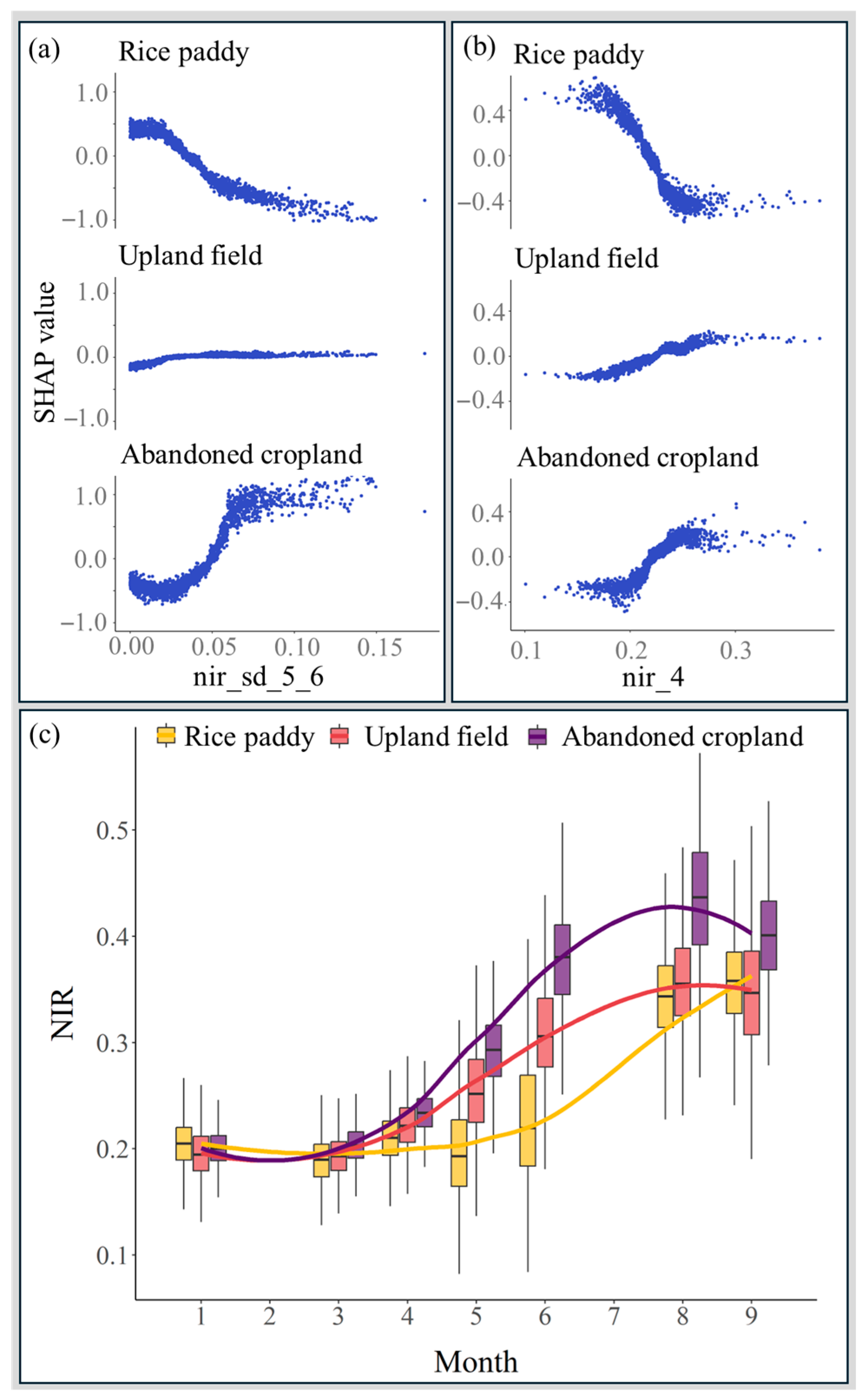
The NIR standard deviation in May–June (nir_sd_5_6) had the highest overall importance and played a critical role in distinguishing rice paddy from abandoned cropland. The NIR band is strongly influenced by chlorophyll reflectance and is known to sensitively capture vegetation vigor and biomass [72]. According to the SHAP dependency plot, rice paddy was more likely to be classified as rice paddy when the May–June NIR standard deviation was low (Figure 7a). In contrast, abandoned cropland showed the opposite trend, with higher values increasing its classification probability. This relationship is consistent with the NIR time-series analysis (Figure 7c). Abandoned cropland showed relatively high NIR reflectance from April onward, maintaining elevated values throughout the growing season with a steeper rate of increase compared to rice paddy and upland fields. Conversely, rice paddy exhibited low NIR reflectance until May–June, followed by a sharp increase in July–August. By September, during the maturation stage, their median NIR reflectance exceeded that of the upland field. In addition, the NIR in April (nir_4) ranked fifth in overall importance and second in importance for rice paddy classification, with lower values generally associated with this class (Figure 7b).
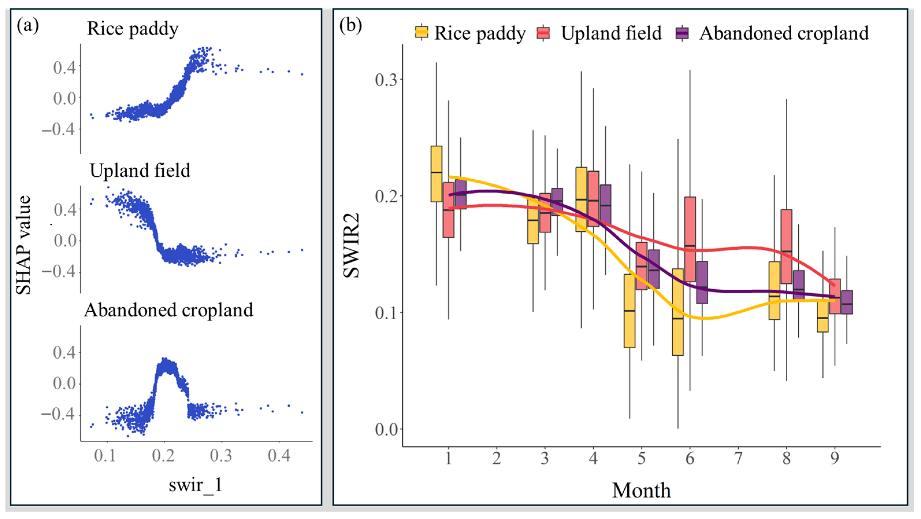
The SWIR2 in January (swir2_1) showed the second-highest overall importance and exhibited consistently high SHAP values across all three classes. The SWIR2 is sensitive to soil and vegetation dryness, mineral composition, and post-fire residues [73,74,75,76]. According to the SHAP dependency plot, rice paddy in January were primarily classified at higher SWIR2 values, whereas abandoned cropland tended to be classified at intermediate values and upland fields at lower values (Figure 8a). The SWIR2 time-series pattern showed a gradual decrease in reflectance across all three classes, beginning in April (Figure 8b). During the growing season, reflectance was highest for upland fields, followed by abandoned cropland and rice paddy.
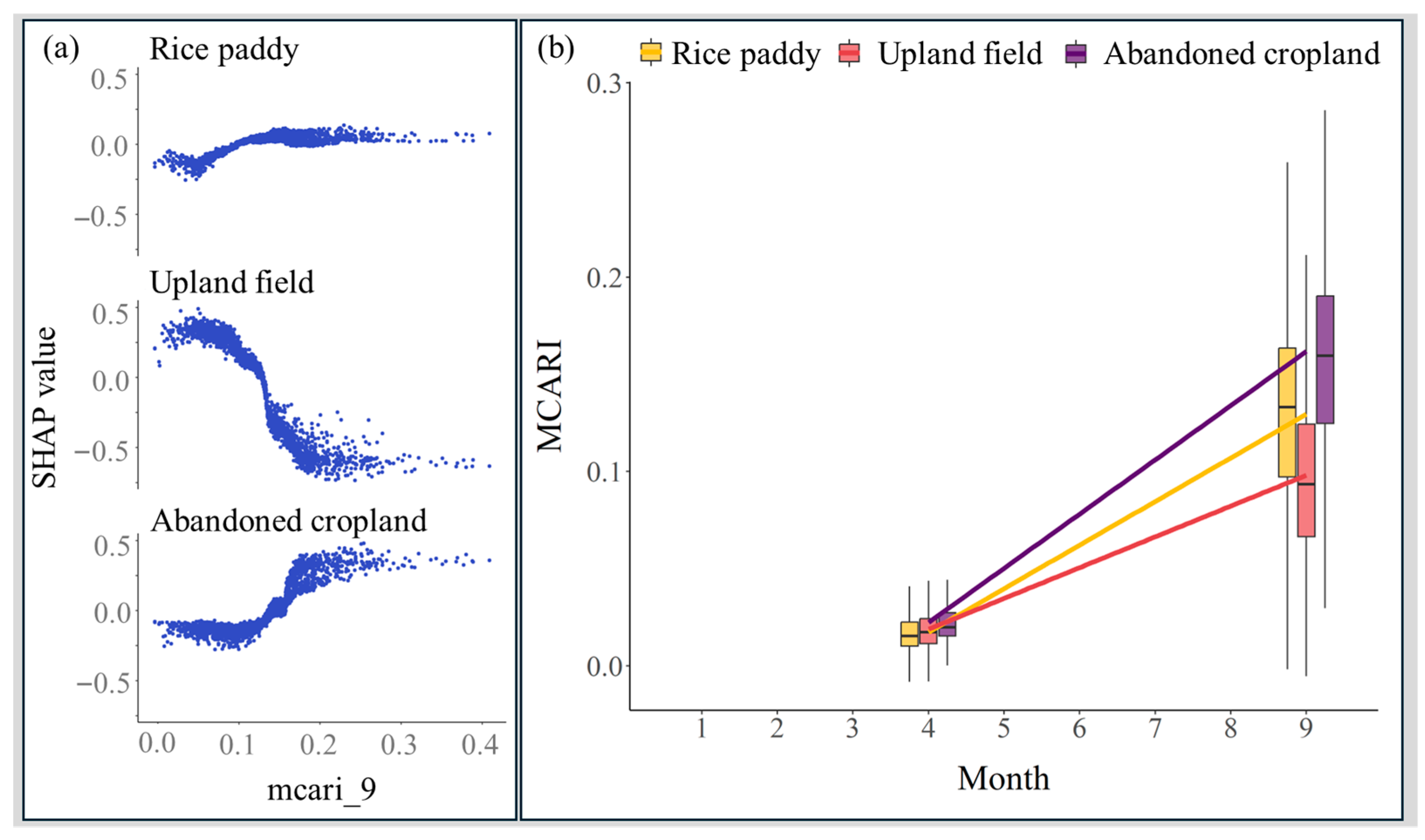
The MCARI in September (mcari_9) showed the third-highest global importance and contributed most strongly to the classification of upland fields. MCARI estimates chlorophyll content using the Red Edge band and is closely related to crop nutritional status and developmental stage [50,77]. The SHAP dependency plot revealed contrasting patterns, where upland fields tended to be classified as such at low MCARI values, whereas abandoned cropland was classified at higher values. (Figure 9a). While MCARI values in April were similar across classes, the increase from April to September was greatest for abandoned cropland, followed by rice paddy and upland fields (Figure 9b).
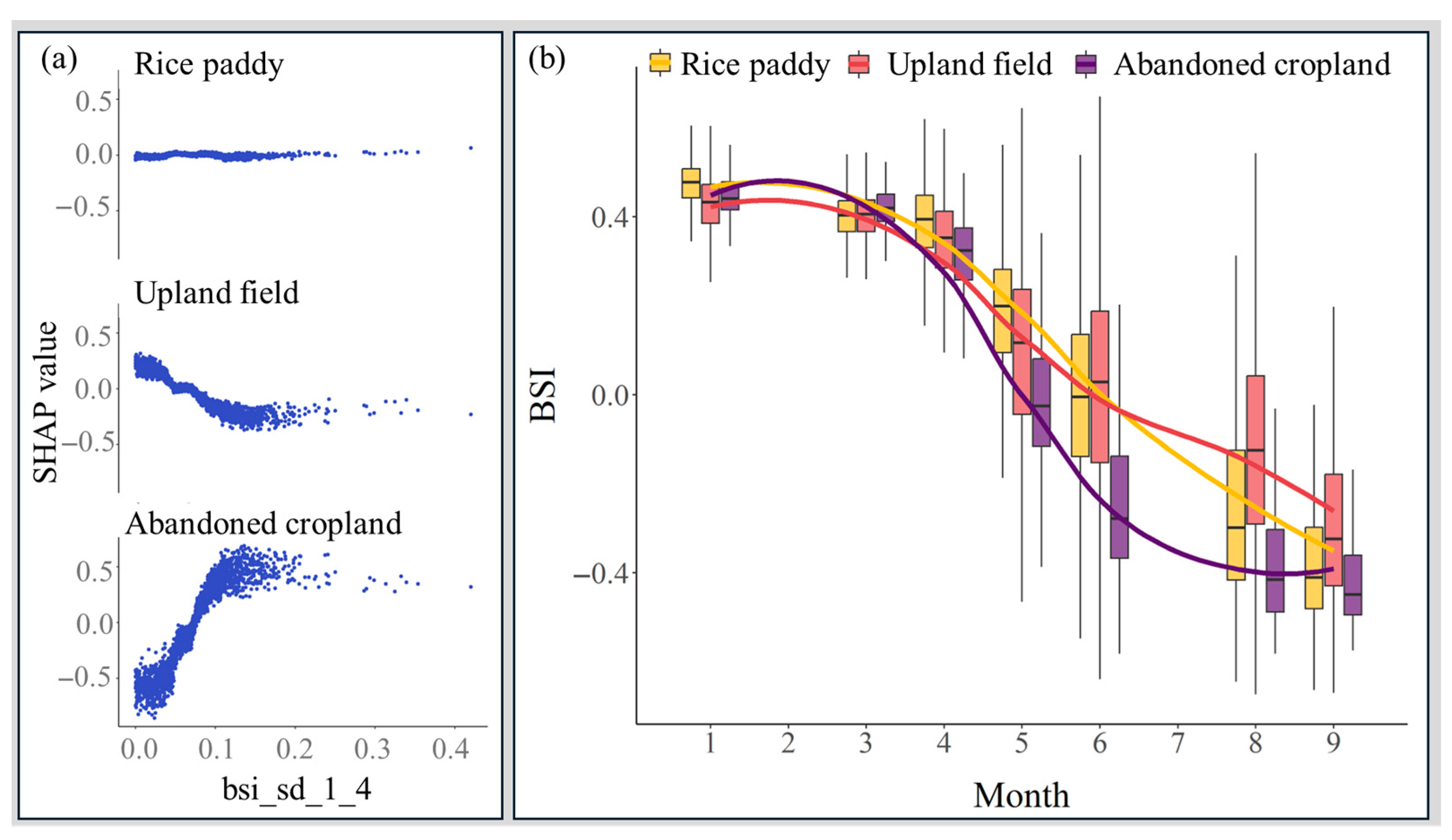
The BSI standard deviation in January and April (bsi_sd_1_4) ranked fourth highest globally and was the second-most influential variable, particularly in identifying abandoned cropland. The BSI represents the proportion of bare soil area, with higher values indicating lower vegetation cover [48]. The January and April BSI standard deviation reflect the degree of change in bare soil exposure during the transition from winter to spring, with larger values indicating greater fluctuations in vegetation cover. The SHAP dependency plot showed that higher BSI standard deviation values were associated with a higher likelihood of classification as abandoned cropland (Figure 10a). Abandoned cropland exhibited the largest change in BSI among the three classes, showing a sharp decrease from January to April compared with rice paddy and upland fields (Figure 10b).

4. Discussion

In this study, we integrated advanced data fusion (HLS) and robust modelling (XGBoost with BBC) to detect challenging abandoned cropland under frequent cloud cover and highly fragmented landscapes. This approach overcomes the time and cost constraints of field survey-based monitoring and develops a continuous large-scale monitoring system even under such challenging conditions. These methodological advancements are particularly relevant under the recent institutional changes to the Farmland Act in South Korea, which emphasize mandatory surveys and strengthened management of abandoned cropland. Consequently, satellite-based detection and monitoring systems are expected to provide data-driven evidence for promoting cropland recultivation, preventing illegal land conversion, and improving overall land-use efficiency.

4.1. Model Performance

Cloudy days in the study area were concentrated during the monsoon season and occurred frequently. It is difficult to reliably obtain high-temporal-resolution optical imagery within the revisit cycle (5–8 days) of a single satellite. Detecting abandoned cropland depends on capturing continuous seasonal changes in vegetation indices [20,78]. Existing abandoned cropland monitoring has primarily relied on time-series imagery from single missions such as Landsat or Sentinel-2 [1,19,79]. To overcome these limitations, this study used HLS time-series imagery, which maintains a 30 m spatial resolution while significantly enhancing temporal resolution (a 2–3-day cycle) by integrating Landsat and Sentinel-2 data [32]. The HLS dataset has recently proven useful in various applications, including crop classification, forest monitoring, and land cover change detection [22,80]. Using HLS data, we constructed continuous monthly phenology datasets that enabled more stable identification of temporal response differences among cropland types.
We utilized 37 time-series core variables selected by the Boruta algorithm and applied an XGBoost model incorporating the BBC to address data imbalance. The extremely low proportion of abandoned cropland as a minority class causes a long-tail distribution in conventional classification algorithms, thereby increasing false negatives [57]. Since missing actual abandoned cropland (false negatives) entails greater policy costs than overdetection, the model in this study was designed to minimize false negatives. To this end, class imbalance in the training samples was corrected using the BBC, and the F 2   s c o r e , which places greater weight on R e c a l l , was employed as the primary evaluation metric. The model achieved an overall accuracy of 0.84 and a C o h e n s   k a p p a coefficient of 0.71, demonstrating strong classification performance. The R e c a l l for abandoned cropland reached 0.94, successfully detecting most actual abandoned areas. Although the P r e c i s i o n was relatively low, indicating that some rice paddy and upland fields were misclassified as abandoned cropland, the falsely detected area accounted for only 2.3% of the total cropland area. Notably, the F 2   s c o r e was 0.84. This score on our primary, R e c a l l -weighted metric reflects the model’s core strength: prioritizing the identification of ‘potentially abandoned cropland’ to ensure actual abandoned sites are not overlooked, even if some active cropland is included in this study. From a policy perspective, the model serves as an effective and efficient monitoring tool. Missing actual abandoned cropland (false negative) can create management blind spots, potentially leading to policy burdens such as unaddressed illegal conversion or management failure. Conversely, misclassifying active cropland as abandoned (false positive) represents a ‘correctable’ cost that can be addressed during secondary assessment, which is an acceptable trade-off given the implications of false negative errors.

4.2. Variable-Wise SHAP Interpretation

Variable contributions derived from SHAP analysis and temporal spectral patterns revealed phenological and optical differences among cropland types. Variations in key spectral features, such as NIR, SWIR2, MCARI, and BSI, effectively explained differences in management intensity and surface cover structure. SHAP interaction values were also examined to explore potential nonlinear interactions between variables. However, no distinct or consistent interaction patterns were observed across the model. Accordingly, this study focused on interpreting the contributions of individual variables and their temporal dynamics.
Variable contributions derived from SHAP analysis and temporal spectral patterns revealed phenological and optical differences among cropland types. The key spectral features, such as NIR, SWIR2, MCARI, and BSI, effectively explained seasonal dynamics in cropland. The NIR standard deviation in May–June (nir_sd_5_6) had the highest importance among all variables, likely reflecting differences in growth patterns driven by rice paddy water coverage and management intensity (Figure 7). Immediately after transplanting (May–Jun), the limited leaf area of rice paddies, combined with strong reflection from flooded water-surface conditions, substantially reduces the NIR spectral response of vegetation [81]. As a result, rice paddy showed the lowest NIR reflectance and the smallest variability. In contrast, abandoned cropland without artificial management showed a rapid expansion of herbaceous vegetation with rising spring temperatures, resulting in a sharp decline in soil exposure and rapid biomass accumulation [82]. Accordingly, the NIR increase after March was most pronounced in abandoned cropland. The upland field maintained a relatively stable level of vegetation cover through continuous management activities such as sowing and weeding, in accordance with the farming schedule. In addition, the NIR in April (nir_4) effectively distinguished rice paddy. This is because rice paddies exhibit minimal vegetation cover during the irrigation preparation period, whereas upland and abandoned cropland show higher reflectance due to early vegetation. In summary, the high importance of NIR features reflects their sensitivity to capturing distinct phenological signatures among rice paddies, upland fields, and abandoned cropland during their early growth stages (e.g., germination, establishment, and vegetative growth) under favorable spring temperature and light conditions. This sensitivity stems from NIR’s strong response to changes in vegetation biomass and leaf internal structure [72].
SWIR2 is highly sensitive to soil and vegetation moisture, particularly dryness, and is more effective than NIR in distinguishing bare soil from senescent vegetation and crop residues [73,74,83]. These materials has lower foliar water content and a higher proportion of non-photosynthetic carbon compounds such as lignin and cellulose, resulting in weaker water absorption and stronger scattering reflectance in the SWIR2 [84,85]. Accordingly, the SWIR2 in January (swir2_1) followed the order of upland fields, abandoned cropland, and rice paddy (Figure 8). In terms of seasonal SWIR2 patterns, rice paddies showed a sharp decrease in reflectance after April due to flooding, while upland fields maintained the highest reflectance throughout the growing season because of its relatively dry and exposed soil. Abandoned cropland showed reflectance similar to upland field in early spring but gradually decreased as herbaceous vegetation growth increased foliar moisture content. Consequently, SWIR2 effectively captured differences in surface cover and crop residues, serving as a particularly valuable variable for detecting abandoned cropland during the winter season. Recent studies have proposed combining SWIR2 with land surface temperature (LST) to distinguish exposed soil from accumulated crop residues [86,87]. Future applications integrating these variables are expected to provide more detailed insights into the residual and unmanaged surface cover characteristics of seasonally abandoned cropland.
MCARI is a vegetation index designed to sensitively capture physiological changes, such as variations in chlorophyll content and photosynthetic activity, by utilizing the Red Edge 1 band [77]. In this study, the MCARI in September (mcari_9) played a decisive role in distinguishing upland fields from abandoned cropland (Figure 9). During this period, canopy coverage reached its maximum, saturating both chlorophyll absorption in the Red band and structural reflection in the NIR [77,88]. As a result, traditional vegetation indices based on Red and NIR combinations are limited in detecting subtle physiological differences among cropland types. In contrast, the Red Edge region, a transitional zone between the chlorophyll absorption and NIR reflectance domains, responds highly sensitive to changes in chlorophyll concentration and photosynthetic capacity. Thus, MCARI more effectively distinguishes physiological variations and vegetation vigor than NIR-based indices and served as a key variable for differentiating upland and abandoned cropland in September.
The BSI standard deviation in January and April (bsi_sd_1_4) represents variability during the transition from winter bare soil conditions to the spring vegetation establishment phase (Figure 10). Abandoned cropland exhibited a pronounced decrease in BSI values as soil exposure rapidly declined with the vigorous spread of vegetation in spring. In contrast, rice paddy and upland fields maintained relatively stable levels of exposed soil under consistent management, resulting in smaller fluctuations. These findings indicate that BSI is highly sensitive to abrupt changes in vegetation cover under unmanaged conditions and can serve as an important indicator of abandoned cropland.
Finally, Sentinel-1 SAR variables were included in the Boruta variable selection process but the combined SHAP contribution of the selected SAR indicators (ratio_mean_5_8, rvi_mean_5_8, ratio_mean_8_9) accounted for only about 3.4% of the total feature importance, indicating that their overall influence on model performance was limited (Figure 5). The SAR imagery was resampled from its original 10 m resolution to 30 m to ensure consistency with other datasets. This resampling process smoothed scattering signals along detailed land-cover structures and boundaries, thereby diluting the backscatter characteristics unique to each cropland type. In addition, only ascending-orbit imagery was available for South Korea [89], resulting in limited observation angles. This restriction likely hindered the detection of subtle surface roughness differences, such as the flooded conditions in rice paddies or the ridge structures in upland fields. Nevertheless, SAR variables complemented optical imagery by capturing surface roughness and moisture-related information that optical sensors could not detect. However, due to limitations in spatial resolution and observation geometry, SAR data alone were insufficient to effectively discriminate among cropland types.

4.3. Limitation of the Study

This study has several limitations related to the structural characteristics of South Korean cropland and data availability. First, Korean agricultural land is characterized by mountainous terrain with steep slopes. Continued subdivisions have resulted in highly fragmented cultivated plots [90]. In addition, the croplands are spatially complex, containing numerous irregular structures such as plastic greenhouses and containers. This spatial complexity, combined with the associated diversity in crop types and growing periods, produces substantial variability in spectral patterns even among adjacent fields. Consequently, these factors may cause boundary ambiguity in satellite image-based classification and are a primary cause of misclassification between cultivated and abandoned cropland [91,92]. Given these limitations, future research could enhance the model by explicitly learning irregular structures as a separate class and by incorporating spatial pattern-recognition techniques, such as object-based segmentation, to enable a more realistic representation of actual cropland boundaries and spatial configurations [20,93]. Furthermore, developing crop-specific phenology databases and adopting fine-grained models capable of independently training multiple crop types would further improve classification accuracy and generalization.
This study faced limitations related to reference data and class imbalance. The proportion of abandoned cropland identified through field surveys accounted for only 2.88% of the total samples, causing a severe class imbalance that affects model generalization. To alleviate this issue, the BBC algorithm was used to address class imbalance. The BBC approach repeatedly increased learning opportunities for the extremely underrepresented abandoned cropland class (2.8%), thereby reducing training bias and improving detection sensitivity ( R e c a l l ). Nevertheless, statistical uncertainty remains due to the absolute scarcity of samples. Future research should focus on developing a long-term database of abandoned cropland and continuously collecting balanced samples across regions, crop types, and seasons to improve the robustness and generalizability of the model.
Using HLS-based time-series imagery and machine learning interpretation techniques (TreeSHAP), we quantitatively analyzed the contribution of each variable and its temporal spectral dynamics. A major strength of this approach is that it enabled the identification of phenological and optical differences among cropland types and the interpretation of seasonal changes in key indices (NIR, SWIR2, MCARI, BSI, etc.). However, the response patterns of certain variables could not be fully explained by a single spectral indicator. For instance, the observation that SWIR2 reflectance in January was higher in rice paddy than in abandoned cropland is presumed to result from a combination of factors, including the presence of winter weeds, crop residues, and differences in soil physical properties [83,94]. To elucidate these mechanisms more precisely, future studies should integrate high-resolution multispectral imagery from drones or ground-based observations to complement analyses of the effects of microenvironmental factors, such as moisture, residue, and soil, on reflectance characteristics. Through this multi-sensor fusion approach, it will be possible to enhance variable-level interpretability and strengthen the model’s physical explanatory power.
Abandoned cropland represents a phenomenon of both national and global significance, making it essential to quantitatively evaluate the model’s transferability across broader spatio-temporal domains. While this study developed the model using imagery from a single crop growth cycle, future validation using multi-year datasets is necessary to reflect the legal and practical definition of abandonment. However, differences in climate, soil, sensor geometry, and land-cover context can lead to variations in reflectance patterns, thereby constraining model transferability. In addition, the monthly aggregation of spectral information adopted in this study may also oversmooth region- and year-specific phenological differences, decreasing phenological fidelity and potentially reducing transferability. To mitigate these issues, recent studies have adopted transfer learning and domain adaptation techniques [95,96], along with preprocessing methods such as relative radiometric normalization (e.g., Pseudo-Invariant Features, PIF) to minimize spectral inconsistencies across sensors, regions, and years [97]. Additionally, gap-filling and temporal smoothing (e.g., Savitzky–Golay filter) applied to original temporal-resolution satellite imagery to ensure temporal continuity and more precisely capture fine-scale phenological patterns [98,99]. Such efforts can enhance model generalization and ensure robust abandoned cropland detection under diverse environmental conditions.

5. Conclusions

This study suggests a practical monitoring framework for the early detection of abandoned cropland in South Korea, where meteorological and topographical characteristics are complex, by integrating time-series satellite imagery and machine learning. Utilizing HLS imagery, which provides high temporal (2–3 days) and spatial (30 m) resolution, the proposed BBC-based XGBoost model effectively distinguishes seasonal spectral and growth stage changes between paddy fields, dry fields, and abandoned croplands. SHAP analysis revealed NIR (May–June), SWIR2 (January), MCARI (September), and BSI (January–April) as key explanatory variables, reflecting distinct temporal and spectral dynamics of abandoned cropland.
Beyond technical performance, this study highlights the potential of interpretable machine learning to improve agricultural land monitoring under complex monsoon-influenced climatic conditions. This approach is applicable to other regions with similar challenges of cloud interference and fragmented land use. The identification of phenology-based spectral indicators further contributes to understanding cropland abandonment and to promoting sustainable agricultural planning.

Author Contributions

Conceptualization, S.P., B.H. and D.W.K.; methodology, S.P., B.H. and D.W.K.; investigation, and writing, S.P., B.H. and S.K.; software, S.P. and S.K.; project administration, writing—review and editing, D.W.K.; and funding acquisition, D.W.K. All authors have read and agreed to the published version of the manuscript.

Funding

This study was conducted with the support of the R&D program for Forest ScienceTechnology (project no. RS-2025-02214405) provided by Korea Forest Service (Korea Forestry Promotion Institute).

Data Availability Statement

Harmonized Landsat and Sentinel-2 is available via the Google Earth Engine platform. The cadastral map is available via the National Geographic Information Institute website (https://www.vworld.kr/dtmk/dtmk_ntads_s002.do?dsId=30563, (accessed on 1 April 2025)), and the land cover is available via the Environmental Geographic Information Service website (https://egis.me.go.kr/req/intro.do, (accessed on 1 April 2025)), but it is not available in English. Requests to access the datasets should be directed to the corresponding author.

Conflicts of Interest

The authors declare no conflicts of interest.

Abbreviations

The following abbreviations are used in this manuscript:
HLSHarmonized Landsat and Sentinel-2
XGBoosteXtreme Gradient Boosting
BBCBalanced Bagging Classifier
XAI explainable artificial intelligence
SHAPSHapley Additive exPlanations

Appendix A

Appendix A.1

To place the BBC method in context with other class-imbalance handling techniques, we additionally applied the SMOTE algorithm. SMOTE was implemented with k = 5, meaning that synthetic samples were generated based on the five nearest neighbors of each minority-class instance. The minority classes were oversampled at a 1:1:1 ratio to match the majority class. Table A1 presents the classification performance of the XGBoost model with SMOTE applied. Overall, the BBC method outperformed SMOTE across all classes, including abandoned cropland, indicating that BBC provides more stable and accurate results in this study.
Table A1. Classification performance of the XGBoost model for rice paddy, upland field, and abandoned cropland with SMOTE applied.
ClassOverall
Accuracy
P r e c i s i o n R e c a l l F 1   S c o r e F 2   S c o r e C o h e n s   K a p p a
Rice paddy0.830.870.800.830.810.68
Upland field0.800.870.830.86
Abandoned cropland0.650.760.700.73

Appendix A.2

Table A2. Definitions and formulas of multispectral and radar indices used in this study.
VariableDescriptionVariableDescription
tcgwd_sd_1_6Standard deviation of TCWGDinv value of January and Juneratio_mean_8_9Mean of VV/VH ratio of August and September
swir1_sd_5_6Standard deviation of SWIR1 reflectance of May and Junetcgwd_sd_4_9Standard deviation of TCWGDinv value of April and September
red_sd_1_4Standard deviation of RED reflectance of January and Aprilred_sd_6_8Standard deviation of RED reflectance of June and August
red_sd_3_5Standard deviation of RED reflectance of March and Mayswir2_1SWIR2 reflectance of January
red_sd_4_5Standard deviation of RED reflectance of April and Maybsi_sd_1_4Standard deviation of BSI value of January and April
tcgwd_sd_1_3Standard deviation of TCWGDinv value of January and Marchnbr_sd_5_8Standard deviation of NBR value of May and August
rvi_mean_5_8Mean RVI value of May and Augustred_sd_5_6Standard deviation of RED reflectance of May and June
tcgwd_sd_5_6Standard deviation of TCWGDinv value of May and Junenbr_sd_5_6Standard deviation of NBR value of May and June
blue_sd_5_9Standard deviation of BLUE reflectance of May and Septembermcari_9MCARI value of September
green_sd_1_5Standard deviation of GREEN reflectance of January and Maynir_sd_1_4Standard deviation of NIR reflectance January and April
tcgwd_sd_3_4Standard deviation of TCWGDinv value of March and Aprilswir2_sd_3_9Standard deviation of SWIR2 Reflectance of March and September
tcgwd_sd_1_4Standard deviation of TCWGDinv value of January and Aprilsavi_sd_5_6Standard deviation of SAVI value of May and June
swir1_sd_5_8Standard deviation of SWIR1 Reflectance of May and Augustnir_4NIR reflectance of April
ndwi_sd_3_4Standard deviation of NDWI value of March and Aprilred_sd_3_6Standard deviation of RED reflectance of March and June
swir1_sd_5_9Standard deviation of SWIR1 Reflectance of May and Septemberratio_mean_5_8Mean of VV/VH ratio of May and August
nbr_sd_5_9Standard deviation of NBR value of May and Septemberndvi_sd_1_3Standard deviation of NDVI value of January and March
nir_sd_3_4Standard deviation of NIR reflectance of March and Aprilswir1_sd_3_8Standard deviation of SWIR1 Reflectance of March and August
nbr_sd_8_9Standard deviation of NBR value of August and Septembernir_sd_5_6Standard deviation of NIR reflectance of May and June
tcgwd_sd_3_8Standard deviation of TCWGDinv value of March and August

References

  1. Liu, T.; Yu, L.; Liu, X.; Peng, D.; Chen, X.; Du, Z.; Zhao, Q. A Global Review of Monitoring Cropland Abandonment Using Remote Sensing: Temporal-Spatial Patterns, Causes, Ecological Effects, and Future Prospects. J. Remote Sens. 2025, 5, 0584. [Google Scholar] [CrossRef]
  2. Prishchepov, A.V.; Schierhorn, F.; Löw, F. Unraveling the Diversity of Trajectories and Drivers of Global Agricultural Land Abandonment. Land 2021, 10, 97. [Google Scholar] [CrossRef]
  3. Vidal-Macua, J.J.; Ninyerola, M.; Zabala, A.; Domingo-Marimon, C.; Gonzalez-Guerrero, O.; Pons, X. Environmental and Socioeconomic Factors of Abandonment of Rainfed and Irrigated Crops in Northeast Spain. Appl. Geogr. 2018, 90, 155–174. [Google Scholar] [CrossRef]
  4. Zhou, T.; Koomen, E.; Ke, X. Determinants of Farmland Abandonment on the Urban–Rural Fringe. Environ. Manag. 2020, 65, 369–384. [Google Scholar] [CrossRef]
  5. Subedi, Y.R.; Kristiansen, P.; Cacho, O. Drivers and consequences of agricultural land abandonment and its reutilisation pathways: A systematic review. Environ. Dev. 2022, 42, 100681. [Google Scholar] [CrossRef]
  6. Gibbs, H.K.; Salmon, J.M. Mapping the world’s degraded lands. Appl. Geogr. 2015, 57, 12–21. [Google Scholar] [CrossRef]
  7. Estel, S.; Kuemmerle, T.; Alcantara, C.; Levers, C.; Prishchepov, A.; Hostert, P. Mapping farmland abandonment and recultivation across Europe using MODIS NDVI time series. Remote Sens. Environ. 2015, 163, 312–325. [Google Scholar] [CrossRef]
  8. Schierhorn, F.; Müller, D.; Beringer, T.; Prishchepov, A.V.; Kuemmerle, T.; Balmann, A. Post-Soviet cropland abandonment and carbon sequestration in European Russia, Ukraine, and Belarus. Glob. Biogeochem. Cycles 2013, 27, 1175–1185. [Google Scholar] [CrossRef]
  9. Hou, J.; Fu, B.J.; Liu, Y.; Lu, N.; Gao, G.Y.; Zhou, J. Ecological and hydrological response of farmlands abandoned for different lengths of time: Evidence from the Loess Hill Slope of China. Glob. Planet. Change 2014, 113, 59–67. [Google Scholar] [CrossRef]
  10. Lasanta, T.; Nadal-Romero, E.; Arnáez, J. Managing abandoned farmland to control the impact of re-vegetation on the environment. The state of the art in Europe. Environ. Sci. Policy 2015, 52, 99–109. [Google Scholar] [CrossRef]
  11. Standish, R.J.; Cramer, V.A.; Hobbs, R.J. Land-use legacy and the persistence of invasive Avena barbata on abandoned farmland. J. Appl. Ecol. 2008, 45, 1576–1583. [Google Scholar] [CrossRef]
  12. Estoque, R.C.; Gomi, K.; Togawa, T.; Ooba, M.; Hijioka, Y.; Akiyama, C.M.; Nakamura, S.; Yoshioka, A.; Kuroda, K. Scenario-Based Land Abandonment Projections: Method, Application and Implications. Sci. Total Environ. 2019, 692, 903–916. [Google Scholar] [CrossRef]
  13. Wang, Y.; Yang, A.; Yang, Q. The extent, drivers and production loss of farmland abandonment in China: Evidence from a spatiotemporal analysis of farm households survey. J. Clean. Prod. 2023, 414, 137772. [Google Scholar] [CrossRef]
  14. Prévosto, B.; Kuiters, L.; Bernhardt-Römermann, M.; Dölle, M.; Schmidt, W.; Hoffmann, M.; Van Uytvanck, J.; Bohner, A.; Kreiner, D.; Stadler, J.; et al. Impacts of Land Abandonment on Vegetation: Successional Pathways in European Habitats. Folia Geobot. 2011, 46, 303–325, Erratum in Folia Geobot. 2011, 47, 117–118. https://doi.org/10.1007/s12224-012-9121-5. [Google Scholar] [CrossRef]
  15. Van der Sluis, T.; Kizos, T.; Pedroli, B. Landscape change in Mediterranean farmlands: Impacts of land abandonment on cultivation terraces in Portofino (Italy) and Lesvos (Greece). J. Landsc. Ecol. 2014, 7, 23–44. [Google Scholar] [CrossRef]
  16. Zhao, X.; Wu, T.; Wang, S.; Liu, K.; Yang, J. Cropland Abandonment Mapping at Sub-Pixel Scales Using Crop Phenological Information and MODIS Time-Series Images. Comput. Electron. Agric. 2023, 208, 107763. [Google Scholar] [CrossRef]
  17. Yoon, H.; Baek, S. Leveraging Temporal, Textural, and Socio-Environmental Features for Accurate Detection of Abandoned Farmland. Remote Sens. Appl. Soc. Environ. 2025, 38, 101598. [Google Scholar] [CrossRef]
  18. He, S.; Shao, H.; Xian, W.; Yin, Z.; You, M.; Zhong, J.; Qi, J. Monitoring cropland abandonment in hilly areas with Sentinel-1 and Sentinel-2 timeseries. Remote Sens. 2022, 14, 3806. [Google Scholar] [CrossRef]
  19. Tran, K.H.; Zhang, H.K.; McMaine, J.T.; Zhang, X.; Luo, D. 10m crop type mapping using Sentinel-2 reflectance and 30 m cropland data layer product. Int. J. Appl. Earth Obs. Geoinf. 2022, 107, 102692. [Google Scholar] [CrossRef]
  20. Wuyun, D.; Sun, L.; Chen, Z.; Li, Y.; Han, M.; Shi, Z.; Ren, T.; Zhao, H. A 10-m resolution dataset of abandoned and reclaimed cropland from 2016 to 2023 in Inner Mongolia, China. Sci. Data 2025, 12, 317. [Google Scholar] [CrossRef]
  21. Hong, C.; Prishchepov, A.V.; Jin, X.; Zhou, Y. Mapping cropland abandonment and distinguishing from intentional afforestation with Landsat time series. Int. J. Appl. Earth Observ. Geoinform. 2024, 127, 103693. [Google Scholar] [CrossRef]
  22. Yoon, H.; Kim, S. Detecting abandoned farmland using harmonic analysis and machine learning. ISPRS J. Photogramm. Remote Sens. 2020, 166, 201–212. [Google Scholar] [CrossRef]
  23. Yeom, J.M.; Jeong, S.; Jeong, G.; Ng, C.T.; Deo, R.C.; Ko, J. Monitoring paddy productivity in North Korea employing geostationary satellite images integrated with GRAMI-rice model. Sci. Rep. 2018, 8, 16121. [Google Scholar] [CrossRef]
  24. Vadrevu, K.P.; Dadhwal, V.K.; Gutman, G.; Justice, C. Remote sensing of agriculture–South/Southeast Asia research initiative special issue. Int. J. Remote Sens. 2019, 40, 8071–8075. [Google Scholar] [CrossRef]
  25. Yin, H.; Brandão, A.J.; Buchner, J.; Helmers, D.; Iuliano, B.G.; Kimambo, N.E.; Lewińska, K.E.; Razenkova, E.; Rizayeva, A.; Rogova, N.; et al. Monitoring cropland abandonment with Landsat time series. Remote Sens. Environ. 2020, 246, 11873. [Google Scholar] [CrossRef]
  26. Peel, M.C.; Finlayson, B.L.; McMahon, T.A. Updated world map of the Köppen-Geiger climate classification. Hydrol. Earth Syst. Sci. 2007, 11, 1633–1644. [Google Scholar] [CrossRef]
  27. Gyeonggi-do Agricultural Research and Extension Services. Status and Implications of Agricultural Production·Demand Matching in Gyeonggi-do; Gyeonggi-do Agricultural Research and Extension Services: Hwaseong, Republic of Korea, 2021. (In Korean) [Google Scholar]
  28. Korea Meteorological Administration. Automated Synoptic Observing System (ASOS)—Material; KMA National Climate Data Center: Seoul, Republic of Korea, 2025; Available online: https://data.kma.go.kr/data/grnd/selectAsosRltmList.do (accessed on 1 October 2025).
  29. Ministry of the Interior and Safety. Status of Administrative Districts and Population in Local Governments; MOIS: Sejong, Republic of Korea, 2025. (In Korean) [Google Scholar]
  30. Ministry of Land, Infrastructure and Transport. Cadastral Map. 2024. Available online: https://www.vworld.kr/dtmk/dtmk_ntads_s002.do?dsId=30563 (accessed on 9 July 2025).
  31. Ministry of Climate, Energy and Environment. Land Cover Map. 2024. Available online: https://egis.me.go.kr/req/intro.do (accessed on 9 July 2025).
  32. Claverie, M.; Ju, J.; Masek, J.G.; Dungan, J.L.; Vermote, E.F.; Roger, J.C.; Skakun, S.V.; Justice, C. The Harmonized Landsat and Sentinel-2 surface reflectance data set. Remote Sens. Environ. 2018, 219, 145–161. [Google Scholar] [CrossRef]
  33. Torres, R.; Snoeij, P.; Geudtner, D.; Bibby, D.; Davidson, M.; Rommen, B. GMES Sentinel-1 mission. Remote Sens. Environ. 2012, 120, 9–24. [Google Scholar] [CrossRef]
  34. Gorelick, N.; Hancher, M.; Dixon, M.; Ilyushchenko, S.; Thau, D.; Moore, R. Google Earth Engine: Planetary-Scale Geospatial Analysis for Everyone. Remote Sens. Environ. 2017, 202, 18–27. [Google Scholar] [CrossRef]
  35. Palchowdhuri, Y.; Valcarce-Diñeiro, R.; King, P.; Sanabria-Soto, M. Classification of multi-temporal spectral indices for crop type mapping: A case study in Coalville, UK. J. Agric. Sci. 2018, 156, 24–36. [Google Scholar] [CrossRef]
  36. Joseph, A.T.; van der Velde, R.; O’Neill, P.E.; Lang, R.H.; Gish, T. Soil Moisture Retrieval During a Corn Growth Cycle Using L-Band (1.6 GHz) Radar Observations. IEEE Trans. Geosci. Remote Sens. 2008, 46, 2365–2374. [Google Scholar] [CrossRef]
  37. Vreugdenhil, M.; Wagner, W.; Bauer-Marschallinger, B.; Pfeil, I.; Teubner, I.; Rüdiger, C.; Strauss, P. Sensitivity of Sentinel-1 backscatter to vegetation dynamics: An Austrian case study. Remote Sens. 2018, 10, 1396. [Google Scholar] [CrossRef]
  38. Kim, Y.; Jackson, T.; Bindlish, R.; Lee, H.; Hong, S. Radar Vegetation Index for Estimating the Vegetation Water Content of Rice and Soybean. IEEE Geosci. Remote Sens. Lett. 2012, 9, 564–568. [Google Scholar] [CrossRef]
  39. Veloso, A.; Mermoz, S.; Bouvet, A.; Le Toan, T.; Planells, M.; Dejoux, J.-F.; Ceschia, E. Understanding the temporal behavior of crops using Sentinel-1 and Sentinel-2-like data for agricultural applications. Remote Sens. Environ. 2017, 199, 415–426. [Google Scholar] [CrossRef]
  40. Yang, Y.Y.; Wu, T.X.; Wang, S.D.; Li, H. Fractional evergreen forest cover mapping by MODIS time-series FEVC-CV methods at sub-pixel scales. ISPRS J. Photogramm. Remote Sens. 2020, 163, 272–283. [Google Scholar] [CrossRef]
  41. Kursa, M.B.; Jankowski, A.; Rudnicki, W.R. Boruta—A system for feature selection. Fundam. Inform. 2010, 101, 271–285. [Google Scholar] [CrossRef]
  42. Strobl, C.; Boulesteix, A.L.; Zeileis, A.; Hothorn, T. Bias in random forest variable importance measures: Illustrations, sources and a solution. BMC Bioinform. 2007, 8, 25. [Google Scholar] [CrossRef]
  43. Altmann, A.; Toloşi, L.; Sander, O.; Lengauer, T. Permutation importance: A corrected feature importance measure. Bioinformatics 2010, 26, 1340–1347. [Google Scholar] [CrossRef]
  44. Kursa, M.B.; Rudnicki, W.R. Feature selection with the Boruta package. J. Stat. Softw. 2010, 36, 1–13. [Google Scholar] [CrossRef]
  45. Tucker, C.J. Red and photographic infrared linear combinations for monitoring vegetation. Remote Sens. Environ. 1979, 8, 127–150. [Google Scholar] [CrossRef]
  46. Huete, A.R. A soil-adjusted vegetation index (SAVI). Remote Sens. Environ. 1988, 25, 295–309. [Google Scholar] [CrossRef]
  47. Key, C.H.; Benson, N.C. Landscape Assessment (LA). In FIREMON Fire Effects Monitoring and Inventory System; Gen Tech Rep RMRS-GTR-164-CD; Lutes, D.C., Keane, R.E., Caratti, J.F., Key, C.H., Benson, N.C., Sutherl, S., Gangi, L.J., Eds.; Department of Agriculture, Forest Service, Rocky Mountain Research Station: Fort Collins, CO, USA, 2006; Volume 164, p. LA-1-55. Available online: https://research.fs.usda.gov/treesearch/24066 (accessed on 20 October 2025).
  48. Rikimaru, A.; Roy, P.S.; Miyatake, S. Tropical Forest cover density mapping. Trop. Ecol. 2002, 43, 39–47. [Google Scholar]
  49. Gao, B.C. NDWI—A normalized difference water index for remote sensing of vegetation liquid water from space. Remote Sens. Environ. 1996, 58, 257–266. [Google Scholar] [CrossRef]
  50. Daughtry, C.S.; Walthall, C.L.; Kim, M.S.; De Colstoun, E.B.; McMurtrey, J.E., III. Estimating corn leaf chlorophyll concentration from leaf and canopy reflectance. Remote Sens. Environ. 2000, 74, 229–239. [Google Scholar] [CrossRef]
  51. Baig, M.H.A.; Zhang, L.; Shuai, T.; Tong, Q. Derivation of a tasseled cap transformation based on Landsat 8 at-satellite reflectance. Remote Sens. Lett. 2014, 5, 423–431. [Google Scholar] [CrossRef]
  52. Fadhil, A.M. Drought mapping using Geoinformation technology for some sites in the Iraqi Kurdistan region. Int. J. Digit. Earth 2011, 4, 239–257. [Google Scholar] [CrossRef]
  53. Huang, C.; Peng, Y.; Lang, M.; Yeo, I.Y.; McCarty, G. Wetland inundation mapping and change monitoring using Landsat and airborne LiDAR data. Remote Sens. Environ. 2014, 141, 231–242. [Google Scholar] [CrossRef]
  54. Kim, Y.; Van Zyl, J.J. A time-series approach to estimate soil moisture using polarimetric radar data. IEEE Trans. Geosci. Remote Sens. 2009, 47, 2519–2527. [Google Scholar] [CrossRef]
  55. Maclin, R.; Opitz, D. An Empirical Evaluation of Bagging and Boosting. In Proceedings of the National Conference on Artificial Intelligence, Providence, RI, USA, 27–31 July 1997; pp. 546–551. [Google Scholar]
  56. Jian, C.; Gao, J.; Ao, Y. A New Sampling Method for Classifying Imbalanced Data Based on Support Vector Machine Ensemble. Neurocomputing 2016, 193, 115–122. [Google Scholar] [CrossRef]
  57. Megahed, F.M.; Chen, Y.-J.; Megahed, A.; Ong, Y.; Altman, N.; Krzywinski, M. The class imbalance problem. Nat. Methods 2021, 18, 1270–1272. [Google Scholar] [CrossRef]
  58. Haixiang, G.; Yijing, L.; Shang, J.; Yuanyue, G.M.H.; Bing, G. Learning from class-imbalanced data: Review of methods andapplications. Expert Syst. Appl. 2017, 73, 220–239. [Google Scholar] [CrossRef]
  59. Vuttipittayamongkol, P.; Elyan, E.; Petrovski, A. On the class overlap problem in imbalanced data classification. Knowl.-Based Syst. 2020, 212, 106631. [Google Scholar] [CrossRef]
  60. Freund, Y.; Schapire, R.E. A Decision-Theoretic Generalization of On-Line Learning and an Application to Boosting. J. Comput. Syst. Sci. 1997, 55, 119–139. [Google Scholar] [CrossRef]
  61. Friedman, J.H. Greedy function approximation: A gradient boosting machine. Ann. Stat. 2001, 29, 1189–1232. Available online: https://www.jstor.org/stable/2699986 (accessed on 20 October 2025). [CrossRef]
  62. Zhang, P.; Jia, Y.; Shang, Y. Research and application of XGBoost in imbalanced data. Int. J. Distrib. Sens. Netw. 2022, 18, 15501329221106935. [Google Scholar] [CrossRef]
  63. Al-Zakhali, O.A.; Zeebaree, S.; Askar, S. Comparative analysis of XGBoost performance for text classification with CPU parallel and non-parallel processing. Indones. J. Comput. Sci. 2024, 13, 1781–1795. [Google Scholar] [CrossRef]
  64. Chen, T.; Guestrin, C. Xgboost: A scalable tree boosting system. In Proceedings of the 22nd ACM Sigkdd International Conference on Knowledge Discovery and Data Mining, San Francisco, CA, USA, 13–17 August 2016; pp. 785–794. [Google Scholar] [CrossRef]
  65. Cohen, J. A Coefficient of Agreement for Nominal Scales. Educ. Psychol. Meas. 1960, 20, 37–46. [Google Scholar] [CrossRef]
  66. Lundberg, S.M.; Lee, S.I. A unified approach to interpreting model predictions. Adv. Neural Inf. Process. Syst. 2017, 30, 4765–4774. [Google Scholar] [CrossRef]
  67. Padarian, J.; McBratney, A.B.; Minasny, B. Game theory interpretation of digital soil mapping convolutional neural networks. Soil 2020, 6, 389–397. [Google Scholar] [CrossRef]
  68. Mangalathu, S.; Hwang, S.H.; Jeon, J.S. Failure mode and effects analysis of RC members based on machine-learning-based SHapley Additive exPlanations (SHAP) approach. Eng. Struct. 2020, 219, 110927. [Google Scholar] [CrossRef]
  69. Chen, T.; He, T.; Benesty, M.; Khotilovich, V.; Tang, Y.; Cho, H.; Chen, K.; Mitchell, R.; Cano, I.; Zhou, T.; et al. Xgboost, version 1.7.11.1; Xgboost: Extreme Gradient Boosting; R Foundation for Statistical Computing: Vienna, Austria, 2025. [CrossRef]
  70. Mayer, M. Shapviz, version 0.10.3; Shapviz: SHAP Visualizations; R Foundation for Statistical Computing: Vienna, Austria, 2025. [CrossRef]
  71. R Core Team. R: A Language and Environment for Statistical Computing; R Foundation for Statistical Computing: Vienna, Austria, 2022; Available online: https://www.R-project.org/ (accessed on 18 April 2025).
  72. Knipling, E.B. Physical and physiological basis for the reflectance of visible and near-infrared radiation from vegetation. Remote Sens. Environ. 1970, 1, 155–159. [Google Scholar] [CrossRef]
  73. Jacques, D.C.; Kergoat, L.; Hiernaux, P.; Mougin, E.; Defourny, P. Monitoring dry vegetation masses in semi-arid areas with MODIS SWIR bands. Remote Sens. Environ. 2014, 153, 40–49. [Google Scholar] [CrossRef]
  74. Yue, J.; Tian, J.; Tian, Q.; Xu, K.; Xu, N. Development of soil moisture indices from differences in water absorption between shortwave-infrared bands. ISPRS J. Photogramm. Remote Sens. 2019, 154, 216–230. [Google Scholar] [CrossRef]
  75. Bishop, J.L.; Lane, M.D.; Dyar, M.D.; Brown, A.J. Reflectance and Emission Spectroscopy Study of Four Groups of Phyllosilicates: Smectites, Kaolinite-Serpentines, Chlorites and Micas. Clay Miner. 2008, 43, 35–54. [Google Scholar] [CrossRef]
  76. Epting, J.; Verbyla, D.; Sorbel, B. Evaluation of remotely sensed indices for assessing burn severity in interior Alaska using Landsat TM and ETM+. Remote Sens. Environ. 2005, 96, 328–339. [Google Scholar] [CrossRef]
  77. Wu, C.; Niu, Z.; Tang, Q.; Huang, W. Estimating chlorophyll content from hyperspectral vegetation indices: Modeling and validation. Agric. For. Meteorol. 2008, 148, 1230–1241. [Google Scholar] [CrossRef]
  78. Volpi, I.; Marchi, S.; Petacchi, R.; Hoxha, K.; Guidotti, D. Detecting Olive Grove Abandonment with Sentinel-2 and Machine Learning: The Development of a Web-Based Tool for Land Management. Smart Agric. Technol. 2023, 3, 100068. [Google Scholar] [CrossRef]
  79. Chen, N.; Tsendbazar, N.-E.; Hamunyela, E.; Verbesselt, J.; Herold, M. Sub-annual tropical forest disturbance monitoring using harmonized Landsat and Sentinel-2 data. Int. J. Appl. Earth Obs. Geoinf. 2021, 102, 102386. [Google Scholar] [CrossRef]
  80. Liu, H.; Zhang, H.K.; Huang, B.; Yan, L.; Tran, K.K.; Qiu, Y.; Roy, D.P. Reconstruction of seamless harmonized Landsat Sentinel-2 (HLS) time series via self-supervised learning. Remote Sens. Environ. 2024, 308, 114191. [Google Scholar] [CrossRef]
  81. de Lima, I.P.; Jorge, R.G.; de Lima, J.L. Remote sensing monitoring of rice fields: Towards assessing water saving irrigation management practices. Front. Remote Sens. 2021, 2, 762093. [Google Scholar] [CrossRef]
  82. Pugnaire, F.I.; Luque, M.T.; Armas, C.; Gutiérraz, L. Colonization processes in semi-arid Mediterranean old fields. J. Arid Environ. 2006, 65, 591–603. [Google Scholar] [CrossRef]
  83. Asner, G.P.; Lobell, D.B. A biogeophysical approach for automated SWIR unmixing of soils and vegetation. Remote Sens. Environ. 2000, 74, 99–112. [Google Scholar] [CrossRef]
  84. Curran, P.J.; Dungan, J.L.; Macler, B.A.; Plummer, S.E.; Peterson, D.L. Reflectance spectroscopy of fresh whole leaves for the estimation of chemical concentration. Remote Sens. Environ. 1992, 39, 153–166. [Google Scholar] [CrossRef]
  85. Jacquemoud, S.; Ustin, S.L.; Verdebout, J.; Schmuck, G.; Andreoli, G.; Hosgood, B. Estimating leaf biochemistry using the PROSPECT leaf optical properties model. Remote Sens. Environ. 1996, 56, 194–202. [Google Scholar] [CrossRef]
  86. Barnes, M.L.; Yoder, L.; Khodaee, M. Detecting winter cover crops and crop residues in the midwest US using machine learning classification of thermal and optical imagery. Remote Sens. 2021, 13, 1998. [Google Scholar] [CrossRef]
  87. Yang, L.; Lu, B.; Schmidt, M.; Natesan, S.; McCaffrey, D. Applications of remote sensing for crop residue cover mapping. Smart Agric. Technol. 2025, 11, 100880. [Google Scholar] [CrossRef]
  88. Sims, D.A.; Gamon, J.A. Relationships between leaf pigment content and spectral reflectance across a wide range of species, leaf structures and developmental stages. Remote Sens. Environ. 2002, 81, 337–354. [Google Scholar] [CrossRef]
  89. S1 Mission. Available online: https://sentiwiki.copernicus.eu/web/s1-mission (accessed on 20 October 2025).
  90. Korea Rural Economic Institute. Agriculture in Korea 2015; Korea Rural Economic Institute: Naju, Republic of Korea, 2015; (In Korean with English Abstract). [Google Scholar]
  91. Sakamoto, T.; Yokozawa, M.; Toritani, H.; Shibayama, M.; Ishitsuka, N.; Ohno, H. A crop phenology detection method using time-series MODIS data. Remote Sens. Environ. 2005, 96, 366–374. [Google Scholar] [CrossRef]
  92. Potgieter, A.B.; Zhao, Y.; Zarco-Tejada, P.J.; Chenu, K.; Zhang, Y.; Porker, K.; Biddulph, B.; Dang, Y.P.; Neale, T.; Roosta, F.; et al. Evolution and application of digital technologies to predict crop type and crop phenology in agriculture. Silico Plants 2021, 3, diab017. [Google Scholar] [CrossRef]
  93. Liu, B.; Song, W. Mapping abandoned cropland using Within-Year Sentinel-2 time series. Catena 2023, 223, 106924. [Google Scholar] [CrossRef]
  94. Schillinger, W.F.; Wuest, S.B. Wheat stubble height effects on soil water capture and retention during long fallow. Agric. Water Manag. 2021, 256, 107117. [Google Scholar] [CrossRef]
  95. Li, J.; Cai, Y.; Li, Q.; Kou, M.; Zhang, T. A Review of Remote Sensing Image Segmentation by Deep Learning Methods. Int. J. Digit. Earth 2024, 17, 2328827. [Google Scholar] [CrossRef]
  96. Ma, Y.; Chen, S.; Ermon, S.; Lobell, D.B. Transfer learning in environmental remote sensing. Remote Sens. Environ. 2024, 301, 113924. [Google Scholar] [CrossRef]
  97. Sadeghi, V.; Ahmadi, F.F.; Ebadi, H. A new automatic regression-based approach for relative radiometric normalization of multitemporal satellite imagery. Comp. Appl. Math. 2015, 36, 825–842. [Google Scholar] [CrossRef]
  98. Chen, Y.; Cao, R.; Chen, J.; Liu, L.; Matsushita, B. A practical approach to reconstruct high-quality Landsat NDVI time-series data by gap filling and the Savitzky–Golay filter. ISPRS J. Photogramm. Remote Sens. 2021, 180, 174–190. [Google Scholar] [CrossRef]
  99. Shao, Y.; Lunetta, R.S.; Wheeler, B.; Iiames, J.S.; Campbell, J.B. An evaluation of time-series smoothing algorithms for land-cover classifications using MODIS-NDVI multi-temporal data. Remote Sens. Environ. 2016, 174, 258–265. [Google Scholar] [CrossRef]
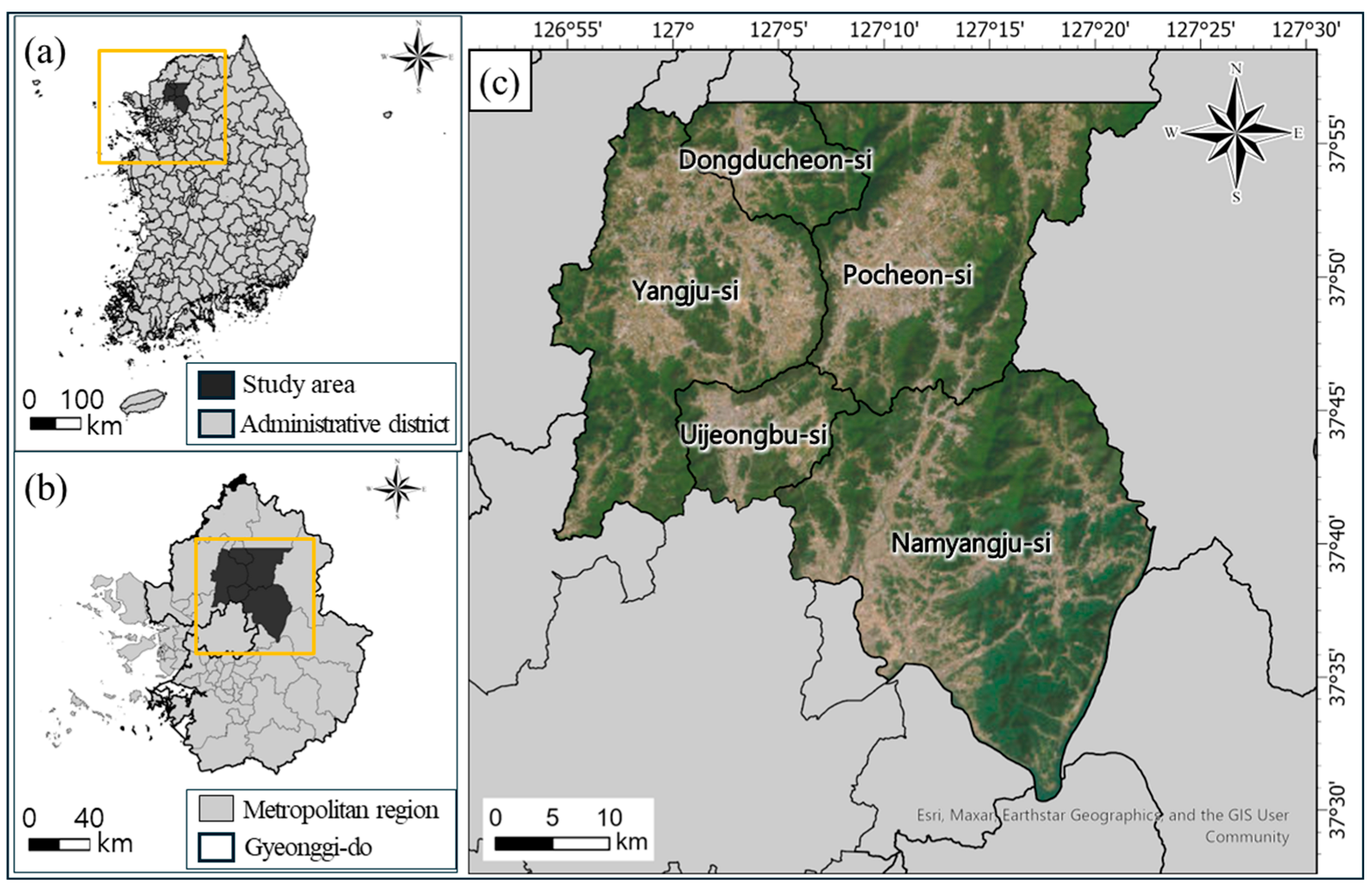
Figure 1. Location of the study area in South Korea. (a) National, (b) regional within Gyeonggi-do Province and the metropolitan region, and (c) local view showing the administrative boundaries. The yellow box in (a) indicates the area shown in (b), and the yellow box in (b) indicates the area shown in (c). The black color represents the study area. (Sources: Esri, Maxar, and Earthstar Geographics).
Agronomy 15 02702 g001
Figure 2. Monthly precipitation and percentage of days classified as “mostly cloudy” or “cloudy” in the study area. “mostly cloudy” refers to total cloud cover of 5.5 or greater on a 0–10 scale, and “cloudy” refers to total cloud cover of 8.5 or greater [28].
Agronomy 15 02702 g002
Figure 3. Overall workflow of the study.
Agronomy 15 02702 g003
Figure 4. (a) Spatial distribution of rice paddies, upland fields, and abandoned croplands used for training and validation in the study area. (bd) Representative field photographs of each cropland type. (Sources: Esri, Maxar, and Earthstar Geographics).
Agronomy 15 02702 g004
Figure 5. Mean absolute SHAP values of the input features.
Agronomy 15 02702 g005
Figure 6. Distribution of SHAP values for input features in the XGBoost-based classification model for cropland types.
Agronomy 15 02702 g006
Figure 7. SHAP dependence plots showing the relationship between SHAP values and (a) the NIR standard deviation in May–June (nir_sd_5_6) and (b) April NIR reflectance (nir_4); (c) Monthly boxplots and smoothed trends of NIR reflectance for rice paddy, upland field, and abandoned cropland.
Agronomy 15 02702 g007
Figure 8. (a) SHAP dependence plot showing the relationship between SHAP values and January SWIR2 reflectance (swir2_1), and (b) monthly boxplots and smoothed trends of SWIR2 reflectance for rice paddy, upland field, and abandoned cropland.
Agronomy 15 02702 g008
Figure 9. (a) SHAP dependence plot showing the relationship between SHAP values and September MCARI reflectance (mcari_9), and (b) monthly boxplots and smoothed trends of MCARI reflectance for rice paddy, upland field, and abandoned cropland.
Agronomy 15 02702 g009
Figure 10. (a) SHAP dependence plot showing the relationship between SHAP values and the BSI standard deviation in January and April (bsi_sd_1_4); (b) Monthly boxplots and smoothed trends of BSI for rice paddy, upland field, and abandoned cropland.
Agronomy 15 02702 g010
Table 1. Summary of major crops, cultivation area, and main growth season for each administrative district in the study area, based on data as of 2020 [27,29].
ProvinceArea (km2)Major CropsCultivation Area (%)Main Growth
Season (Month)
Dongducheon-si95.67Perilla39.026–9
Young Summer RadishMultiple crops
Namyangju-si458.13Perilla16.196–9
SpinachMultiple crops
Pocheon-si827.23Rice39.555–8
SpinachMultiple crops
Uijeongbu-si81.55Rice28.145–8
Perilla6–9
Yangju-si310.49Rice46.635–8
Perilla6–9
Table 3. Classification performance of the XGBoost model for rice paddy, upland field, and abandoned cropland.
ClassOverall
Accuracy
P r e c i s i o n R e c a l l F 1   S c o r e F 2   S c o r e C o h e n s   K a p p a
Rice paddy0.840.900.800.850.820.71
Upland field0.820.880.850.88
Abandoned cropland0.540.940.690.84
Disclaimer/Publisher’s Note: The statements, opinions and data contained in all publications are solely those of the individual author(s) and contributor(s) and not of MDPI and/or the editor(s). MDPI and/or the editor(s) disclaim responsibility for any injury to people or property resulting from any ideas, methods, instructions or products referred to in the content.