Article

A Multi-Level Segmentation Method for Mountainous Camellia oleifera Plantation with High Canopy Closure Using UAV Imagery

1
School of Natural Resources and Surveying, Nanning Normal University, Nanning 530100, China
2
University Engineering Research Center of “Satellite+” Space AI Intelligent Governance of Natural Resources, Nanning Normal University, Nanning 530100, China
3
Guangxi Engineering Research Center for Smart Monitoring and Governance of Agricultural Land, Nanning 530100, China
4
School of Artificial Intelligence, China University of Geosciences (Beijing), Beijing 100083, China
5
Hebei Key Laboratory of Geospatial·Digital·Twin and Collaborative Optimization, Beijing 100083, China
6
Guangxi Environmental Protection Industry Investment Group Co., Ltd., Nanning 530200, China
*
Author to whom correspondence should be addressed.
Agronomy 2025, 15(11), 2522; https://doi.org/10.3390/agronomy15112522
Submission received: 18 July 2025 / Revised: 11 October 2025 / Accepted: 17 October 2025 / Published: 29 October 2025
(This article belongs to the Section Precision and Digital Agriculture)

Abstract

Camellia oleifera is an important economic tree species in China. Accurate estimation of canopy structural parameters of C. oleifera is essential for yield prediction and plantation management. However, this remains challenging in mountainous plantations due to canopy occlusion and background interference. This study developed a multi-level object-oriented segmentation method integrating UAV-based LiDAR and visible-light data to address this issue. The proposed approach progressively eliminates background objects (bare soil, weeds, and forest gaps) through hierarchical segmentation and classification in eCognition, ultimately enabling precise canopy delineation. The method was validated in a high-canopy-closure plantation characterized by a mountainous area. The results demonstrated exceptional performance; canopy area extraction and individual plant extraction achieved average F-scores of 97.54% and 91.69%, respectively. The estimated tree height and mean crown diameter were strongly correlated with field measurements (both R2 = 0.75). This study provides a method for extracting the parameters of C. oleifera canopies that is suitable for mountainous regions with high canopy closure, demonstrating significant potential for supporting digital management and precision forestry optimization in such wooded areas.

1. Introduction

Camellia oleifera, an important woody oil tree species in China, possesses significant economic value and ecological benefits [1,2]. Its cultivation area has been expanding in recent years. The Guangxi Zhuang Autonomous Region is a crucial production base for China’s C. oleifera industry [3]. Benefiting from its subtropical monsoon climate and karst topography, the region has developed C. oleifera into a pillar of ecological industry for rural revitalization. However, mountains and hills constitute 76.54% of Guangxi’s total area [4]. Local mature C. oleifera forests in these mountainous regions often exhibit high canopy closure (defined as greater than 0.7), leading to a crowded stand structure, poor ventilation and light penetration, and increased susceptibility to pests and diseases, which constrains yield improvement [5]. Concurrently, inconvenient transportation and high habitat heterogeneity in mountainous areas significantly increase management difficulty and cost [6], make mechanization challenging, and result in high labor costs [7,8]. These challenges create an urgent need for crown monitoring methods tailored to mountainous, high-canopy-closure C. oleifera plantations to enable scientific and intensive management.
The tree crown, as the core part of physiological activities, has morphological parameters that directly reflect individual tree growth status and stand spatial structure. These parameters are crucial for biomass estimation, photosynthetic capacity assessment, and competition analysis [9,10,11]. While satellite remote sensing offers broad-scale monitoring capabilities, its applications in hilly terrains are constrained by long revisit cycles, coarse spatial resolution, and susceptibility to cloud interference [12]. Unmanned Aerial Vehicle (UAV) technology, as a transformative tool in forestry, effectively bridges the technical gap between ground surveys and satellite remote sensing due to its advantages, such as strong mobility, long endurance, and the ability to acquire high-resolution data [13]. UAVs can also acquire centimeter-level imagery, providing a data foundation for precisely extracting crown parameters. Significant progress has been made in crown segmentation methods based on high-resolution UAV imagery. These capabilities make UAVs particularly suitable for extracting canopy parameters in mountainous areas with high canopy closure [14]. Existing methods can be broadly categorized into three types: traditional image processing methods, deep learning methods, and multi-source data fusion methods.
Traditional image processing methods primarily rely on combining Canopy Height Models (CHMs) with morphological algorithms, including local maxima filtering, the watershed algorithm, the region growing algorithm, and level set methods [8,15,16]. These methods offer high computational efficiency and extraction accuracy under low canopy closure conditions, but their segmentation accuracy decreases significantly under high canopy closure [15,16]. Furthermore, traditional methods are prone to the “salt-and-pepper effect” (i.e., fragmented segmentation caused by pixel-level noise in high-resolution imagery) [17]. Object-Based Image Analysis (OBIA), which forms image objects with homogeneous features through multi-scale segmentation, demonstrates unique advantages in complex crown segmentation [18]. This object-based approach inherently mitigates the salt-and-pepper effect by averaging intra-object spectral data and utilizing contextual features (e.g., shape, texture); more importantly, it better captures the integrity and boundaries of structurally complex canopies [18]. As a result, OBIA effectively achieved high-precision extraction of crown coverage and forest structural parameters in poplar forests in Northern Shaanxi [19]. Furthermore, by integrating multi-dimensional features, including spectral, geometric, and topological characteristics, OBIA has enabled the classification and crown recognition of six tree species in the loess region of Western Shanxi [20]. Deep learning methods have somewhat alleviated the issue of crown occlusion [21]. Ferro et al. [22] found that while OBIA methods were prone to misclassifying shadows, deep learning approaches like Mask R-CNN and U-Net achieved superior accuracy for crown recognition in vineyards. Moreover, their evaluation for crop vigor mapping revealed a fundamental principle: enhanced canopy delineation, particularly in handling shadows and background, is essential for obtaining reliable vegetation indices. The combination of U-Net with marker-controlled watershed segmentation achieved individual tree segmentation for Chinese fir [9] and Tianshan spruce [14]. Combining Convolutional Neural Networks (CNNs) with mask regions enabled high-precision extraction of tree height and crown parameters [23]. However, these methods require large-scale annotated samples, and their generalization capability across different tree species scenarios remains limited.
Multi-source data fusion technology, by integrating LiDAR and RGB image data, can capture forest vertical structure information, enhancing tree height extraction and canopy segmentation capabilities [24]. Several studies indicate that for medium- and high-canopy-closure stands, methods based on CHMs hold advantages over direct point-cloud-based individual tree segmentation [25,26]. Regarding crown identification, Fu et al. [27] proposed a hybrid segmentation method combining region growing with super pixel-weighted fuzzy clustering, achieving the efficient contour extraction of individual trees; Quan et al. [28] utilized UAV LiDAR data to achieve the fine modeling of larch forest canopies, effectively distinguishing between full-crown and upper-crown structures. For canopy parameter inversion, Wei et al. [29] and Wang et al. [30] used watershed segmentation and the hierarchical flood algorithm, respectively, for individual tree parameter extraction in mangroves and coniferous forests. Furthermore, Huang et al. [31] significantly improved individual tree segmentation accuracy and terrain adaptability under complex mountainous conditions by refining filtering algorithms and comparing various segmentation methods. These studies fully leverage LiDAR’s advantages in acquiring high-precision 3D point clouds and characterizing vertical canopy structure while simultaneously utilizing the rich spectral and textural features of optical imagery and compensating for the limitations of single data sources in terms of spectral information or occlusion resistance. Through their complementary advantages, they significantly enhance the accuracy and robustness of crown segmentation and parameter inversion in complex environments, providing reliable technical support for research on high-density canopy vegetation.
Current research in C. oleifera information extraction is subject to several inherent limitations. Studies using satellite platforms (e.g., Sentinel-1/2, Gaofen series) primarily achieve large-scale forest identification by integrating spectral, textural, and temporal features; however, their spatial resolution remains insufficient for fine-scale monitoring at the individual tree level [32,33,34,35]. Research based on UAV platforms provides greater spatial detail, yet most applications focus predominantly on fruit-related tasks such as picking, counting, and maturity assessment [36,37,38,39,40]. It is also noteworthy that the limited number of studies on canopy parameter extraction have generally been validated only in flat, well-managed plantations with uniform crown structure. For instance, although Yu et al. [41] and Wu et al. [42] have successfully applied methods such as ResU-Net and watershed segmentation, these approaches have been tested only under simplified conditions and lack validated robustness in environments with mountainous terrain and high-canopy-closure.
These limitations become particularly pronounced in the specific context of mountainous C. oleifera plantations with high-canopy-closure. Firstly, the dense interlocking and overlapping of adjacent crowns in both horizontal and vertical dimensions adversely affect the performance of CHM-based algorithms in detecting individual tree boundaries, frequently resulting in multiple crowns being misclassified as a single “super-crown”. This leads to substantial underestimation of tree numbers and overestimation of crown dimensions [13]. Secondly, the dense canopy attenuates laser pulse penetration, compromising the accuracy of DEM generation and consequently undermining CHM reliability [43]. Furthermore, high-closure stands are predominantly distributed in topographically complex mountainous regions, where terrain correction errors can distort CHM data, causing crown deformation and mislocation on slopes and further exacerbating segmentation difficulties [44]. Addressing these challenges requires synergistic advancements in both data sources (e.g., LiDAR integration) and analytical algorithms (e.g., multi-level segmentation).
As a result, the accurate segmentation of individual tree crowns in mountainous C. oleifera plantations with high canopy closure remains a persistent challenge. This gap leads to a critical shortage of suitable management technologies for major C. oleifera planting areas such as those in Guangxi. These conditions generate an urgent need for precision monitoring solutions that can effectively handle topographic variation and crown occlusion. To address this gap, this study proposes a multi-level segmentation method that integrates UAV-based LiDAR and visible-light data. The approach is specifically designed to tackle crown segmentation challenges in mountainous environments, thereby providing technical support for precision management of this important economic species.
This study takes the C. oleifera demonstration planting base in Gaofeng Forest Park, Nanning, Guangxi, as the study area. Aiming at mountainous terrain and high-canopy-closure conditions, we propose a multi-level canopy segmentation method based on UAV imagery. The research primarily includes two objectives: (1) construct a multi-source feature set through LiDAR and visible light image fusion to establish an object-based hierarchical segmentation process for precise crown extraction and background removal; and (2) create a dedicated segmentation algorithm for high-closure conditions to effectively improve segmentation accuracy in dense canopies.

2. Materials and Methods

2.1. Study Area

The C. oleifera demonstration forest is located in Compartment 15 of Gaofeng Forest Park (108°21′42″ E, 22°57′26″ N), Nanning, GXZAR, in southern China (Figure 1). The site features red soil (pH 5.2–5.8) and elevational gradients ranging from 118 to 237 m, representing typical karst hill topography. The park exhibits a subtropical monsoon climate characterized by hot, rainy summers and mild, dry winters. The annual precipitation ranges from 1100 to 1700 mm, with over 60% occurring between June and August. The mean annual temperature is 21.7 °C (12.8 °C in January, 28.6 °C in July), with the annual evapotranspiration ranging from 1100 to 1300 mm, 40% of which occurs from June to August.
The demonstration forest, dominated by the C. oleifera cultivar “Cenruan 3”, was established in May 2009 and reached 14 years of age during data acquisition. The initial planting density was 2 m × 3 m (1665 plants/ha), and it was reduced to 840 plants/ha after thinning in 2015. The favorable soil conditions and hydrothermal climate promoted rapid forest growth, resulting in current stand characteristics, including a mean diameter at breast height (DBH) of 7.20 cm (max. 12.70 cm) and an average tree height of 4.65 m. These growth patterns have collectively led to dense understory weeds and highly closed canopies, making the site ideal for testing canopy segmentation algorithms regarding their ability to delineate overlapping crowns and suppress background noise. Visual interpretation of aerial imagery revealed an average canopy closure of 0.85 across the sample plots. The 20 cm resolution Digital Elevation Model (DEM) derived from UAV LiDAR point clouds revealed significant topographic variation, with an average slope of 30.19° calculated using ArcGIS Pro 3.0.2 This complex terrain makes the location a suitable testing ground for validating the adaptability and robustness of UAV-based methods in non-flat areas.
To evaluate the technical applicability of the method, four 60 m × 60 m standard plots were established across elevation gradients: two as experimental zones and two as validation zones (see Figure 1c–g for locations and Table 1 for details). The plots exhibited three key characteristics that challenged remote sensing analysis: high canopy density (>0.70 crown overlap), complex background features (including weeds, bare soil, and forest gaps), and significant topographic variation (25–35° slopes). These conditions collectively form a testing environment that closely resembles real production scenarios, providing an ideal setting for validating the robustness and adaptability of canopy segmentation methods.

2.2. Technical Workflow

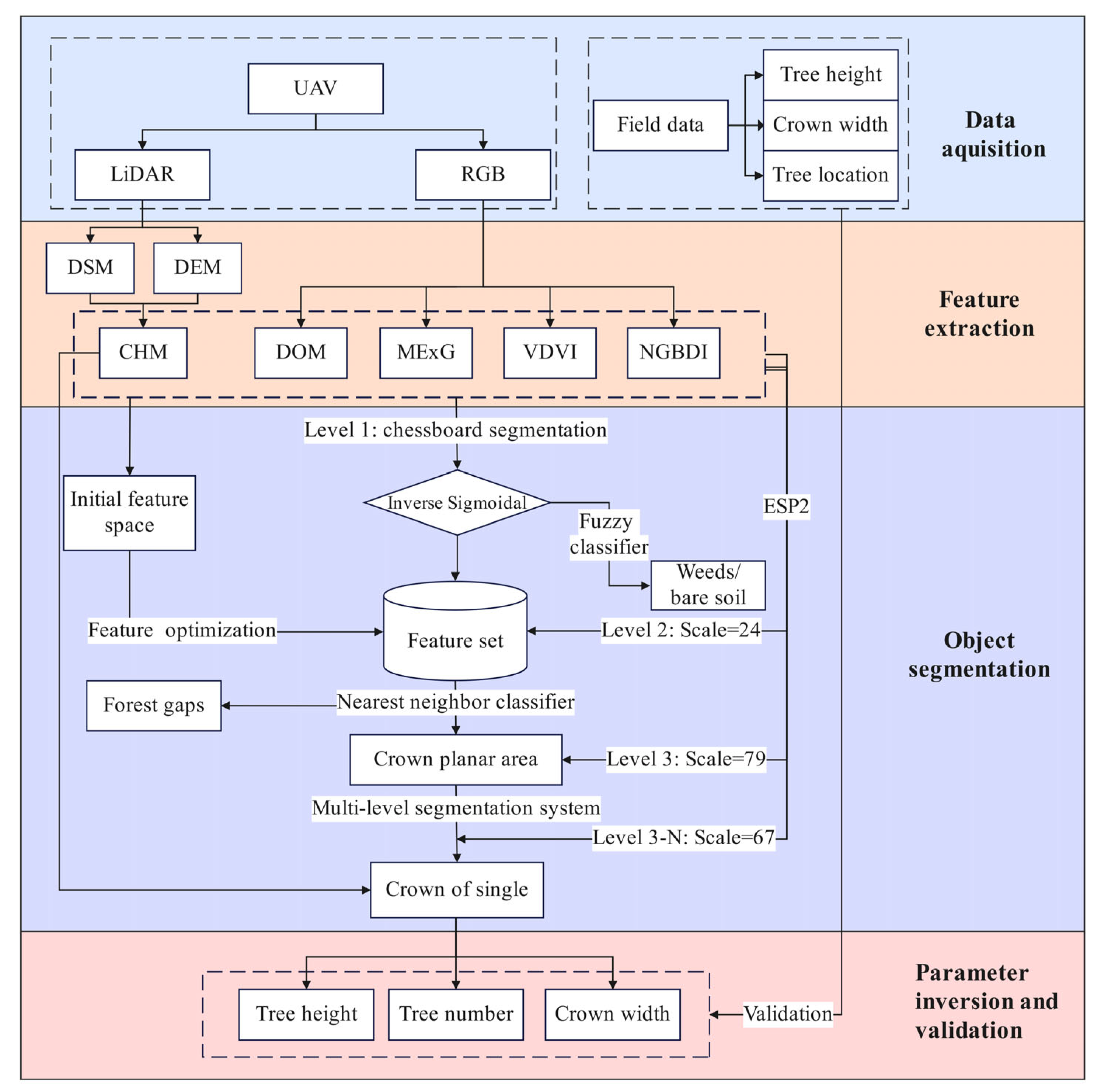
The research framework (Figure 2) comprises the following steps.
(1)
Data acquisition
LiDAR point cloud data and RGB images were acquired using a Hi-Target L120 UAV. Field measurements included tree height, crown width (including east–west and north–south crown width), and tree locations (see Section 2.3 for details).
(2)
Feature extraction
A CHM was computed from the LiDAR point cloud. A Digital Orthophoto Map (DOM) was generated based on the visible light imagery. Spectral features derived from RGB bands and visible vegetation indices (MExG, VDVI, NGBDI) were analyzed. These features were integrated to construct a multi-dimensional feature space (see Section 2.4 for details).
(3)
Object-based fuzzy classification (first-level segmentation)
The objective of the first-level segmentation is to recognize bare soil/weeds areas. To this end, scale and CHM thresholds were compared and an optimal combination was selected. A fuzzy classification method within eCognition was then employed to perform a soft segmentation of the feature space, which successfully suppressed the background objects (see Section 2.5).
(4)
Object-based nearest-neighbor classification (second-level segmentation)
The objective of the second-level segmentation is to distinguish canopy objects from residual noise. The ESP2 tool determined the optimal segmentation scale for C. oleifera and background objects. Image segmentation was performed using the optimal scale parameter identified for forest gaps. Subsequently, a stable and optimized feature set was constructed, and a nearest-neighbor classifier was employed to eliminate interference from forest gaps, ultimately achieving precise extraction of planar canopy areas (see Section 2.6.1, Section 2.6.3 and Section 2.6.4 for details).
(5)
Multi-level segmentation system (third-level segmentation)
The third-level segmentation implements a multi-level hierarchical framework specifically designed for delineating interconnected canopies, which employs mean area and standard deviation thresholds at each segmentation level to progressively refine canopy planar segmentation while effectively controlling error propagation (see Section 2.6.2 for details).
(6)
Parameter extraction and accuracy validation
Based on individual tree crowns, the tree height and crown width (including the east–west and north–south crown width) were extracted. These parameters were then validated against field-measured data to assess accuracy (see Section 2.7 for details).

2.3. Data Acquisition

2.3.1. UAV Mission Configuration

A Hi-Target Longteng L120 multirotor UAV equipped with an ARS 1000P LiDAR sensor (Guangzhou Hi-Target Navigation Technology Co., Ltd., Guangzhou, China) was deployed to perform aerial surveying on 26 September 2022. The flight was conducted from 11:00 to 12:00 local time under cloudless conditions to minimize shadow-related noise in the data. The sensor integrated an RGB camera (Table S1) and a Hi-POS inertial navigation system (Table S2), enabling centimeter-level positioning accuracy.
The flight was carried out in an S-form trajectory for continuous image acquisition. In order to obtain an efficient mosaic image from the UAV imagery while ensuring sufficient feature points for matching, avoiding stitching gaps, and maintaining flight efficiency, the flight path was configured with 90% forward overlap and 65% side overlap between adjacent strips. Additionally, the camera was set to a nadir-facing orientation (90° viewing angle) to minimize projection distortions. The coordinate system was set at CGCS2000 with a central longitude of 108°. The flight height of 250 m was selected to balance data quality and operational efficiency, achieving a ground sampling distance (GSD) of 0.042 m with the 61 million pixels camera while maintaining sufficient point cloud density for the LiDAR system. A total of 482 images were acquired, with simultaneous GNSS-RTK base station deployment (1 Hz sampling rate) to enhance georeferencing accuracy. When taking the photos, the UAV also simultaneously recorded the position information of the flight, including the coordinates, altitude, and viewing angle of the image. The technical specifications of the UAV camera and the details of the UAV flight campaigns are presented in Table S3.
Visible-light imagery was processed using Agisoft Metashape Professional 1.8.5 to generate a DOM with an initial resolution of 0.42 cm through feature matching and dense point cloud reconstruction, and the result was subsequently resampled to a resolution of 0.05 m. LiDAR data underwent trajectory correction, point cloud merging, and spatial–spectral registration with optical imagery using the HD Data Combine3.4.5. High-altitude and low-altitude outliers were removed to produce true-color point clouds for multimodal analysis. The point cloud density within the study area reached 122 points/m2.

2.3.2. Field Data Acquisition

Field sampling was conducted on 26 September 2022. A systematic random sampling method was employed to establish 100 sample C. oleifera trees within the study area. Based on Google Earth imagery and existing topographic maps, the boundaries of sample plots were initially delineated. Within each sample plot, 20–30 sampling points were systematically distributed at 5–10 m intervals to ensure spatial uniformity. Each sample tree was precisely georeferenced using a GNSS RTK receiver (South Surveying & Mapping Technology Co., Ltd., Guangzhou, China), and tree height, east–west crown diameter, and north–south crown diameter was measured with a hypsometer (accuracy: 0.1 m). This sampling strategy ensured comprehensive coverage of topographic variations across the study area, and the collected data served as benchmark references for validating canopy parameter extraction results.

2.4. Data Processing and Feature Analysis

2.4.1. Canopy Height Model (CHM) Generation

The Digital Surface Model (DSM) represents the top elevation model of all objects on the Earth’s surface. It was generated through multi-flightline fusion, denoising, and interpolation of the UAV-LiDAR point clouds. The digital elevation model (DEM) represents elevation information of the bare-earth surface. It was extracted from the classified ground points using an improved progressive encryption triangulated irregular network (TIN) densification filtering algorithm. A high-precision CHM was derived by subtracting the digital elevation model (DEM) from the digital surface model (DSM) [36]. The formulas are shown in (1) to (3).
DSM = { ( x i ,   y j ,   z ij ) } ( i = 1 ,     2 ,     3 , ,   n ;   j = 1 ,   2 ,   3 ,   ,   m )
DEM = { ( x i ,   y j ,   H ij ) } ( i = 1 ,     2 ,     3 , ,   n ;   j = 1 ,   2 ,   3 ,   ,   m )
CHM = DSM DEM
In the formula, x and y represent planar coordinates, z denotes the elevation of the Earth’s surface features, H indicates the ground point elevation, n is the number of image rows, and m is the number of image columns.
To optimize ground point classification and enhance DEM accuracy, key parameters, including the maximum building height, maximum terrain angle, iteration distance, and iteration angle, were meticulously adjusted. This process effectively identified and filtered out non-ground outliers (e.g., low vegetation and small objects). Furthermore, a manual inspection and correction procedure was implemented to rectify any misclassified points, ensuring the fidelity of the ground model.
The resulting CHM has a spatial resolution of 5 cm, providing a detailed representation of the canopy’s vertical structure. This high-resolution CHM enables the clear delineation of crown stratification and serves as a critical data layer for subsequent crown identification, segmentation, and individual tree enumeration. To quantitatively assess the accuracy of the generated CHM, the tree heights derived from the CHM were compared with field-measured tree heights. Statistical metrics, including the R-squared, Root Mean Square Error (RMSE), and Mean Absolute Error (MAE), were calculated to evaluate the performance of the CHM-derived height estimates (see Section 3.8 for the results).

2.4.2. RGB and Vegetation Index Analysis

The UAV-derived true-color imagery comprised red (R), green (G), and blue (B) bands. To distinguish C. oleifera from background features, pixel values were normalized to the range of 0–255, and the spectral characteristics of the RGB bands were analyzed. The visible-light vegetation indices are less affected by atmospheric aerosols and water vapor, making them more suitable for high-frequency monitoring tasks using low-altitude platforms such as drones. These indices are calculated based on the reflectance of visible light bands, eliminating the reliance on near-infrared bands. They offer advantages such as low equipment costs, ease of operation, and strong real-time performance. The visible vegetation indices used in this study and their advantages are summarized in Table 2. In the formulas presented in Table 2, r, g, and b represent the normalized pixel values of the red, green, and blue bands in the visible light imagery, respectively.
Based on visually interpreted regions of weeds, bare soil, forest gaps, and C. oleifera, random samples were generated within the experimental area using ArcGIS Pro 3.0.2 A minimum sampling distance of 5 m was implemented to mitigate spatial autocorrelation, which exceeds the average crown diameter (4 m) of the studied trees. A total of 30 C. oleifera samples, 20 weed samples, 20 soil samples, and 20 forest gap samples were created. To characterize the differences between background features and C. oleifera, three parameters were selected for statistical analysis: the coefficient of variation (CV), the coefficient of relative difference (CRD), and the Jeffries–Matusita (J-M) distance. The calculations for the CV and CRD are provided in Table S4, while the J-M distance is defined as follows:
J M i j = 2 ( 1 e B )
B = 1 8 ( μ i μ j ) 2 2 σ i 2 + σ j 2 + 1 2 ln ( σ i 2 + σ j 2 2 σ i σ j )
μ i and μ j represent the mean values of feature in class i and class j, respectively, while σ i and σ j denote the variances of the feature in class i and class j. Lower CV and higher CRD values indicate stronger separability between C. camellia and background features. The Jeffries-Matusita (J-M) takes into account both the within-class dispersion and the between-class separation. A common interpretation of J-M values is as follows: JM < 1.0: poor separability, 1.0 < JM < 1.8: moderate separability, JM > 1.8: good separability [48].

2.5. Object-Based Fuzzy Classification

2.5.1. Chessboard Segmentation

Chessboard segmentation, a top-down image partitioning method, divides entire scenes or regions of interest into regularly arranged square units of uniform size. The tested segmentation sizes of 5, 10, and 15 pixels were chosen with reference to the eCognition’s default value (10 pixels), including one finer (5 pixels) and one coarser (15 pixels) scale to comprehensively evaluate the impact of scale on segmenting bare soil and weeds. The optimal parameter was determined by evaluating identification accuracy against visual interpretation results.

2.5.2. Fuzzy Classification

Based on the fuzzy classification method within the eCognition platform, this study achieves a soft partition of the feature space by constructing membership functions. For the weed/bare soil category, corresponding membership functions were defined based on prior knowledge. The classification results were determined by calculating the degree to which image objects belong to this category and applying the principle of maximum membership.
There exists a significant vertical structural difference between bare soil/weeds and C. oleifera canopies: C. oleifera canopies generally exhibit greater height, whereas weeds and bare soil are closer to the ground surface, with their CHM values approaching zero. Field measurements indicate that the minimum canopy height of C. oleifera plants is approximately 2.57 m, and bare soil areas can be further distinguished with the assistance of a DEM. Therefore, the CHM serves as a critical feature for differentiating these feature categories.
This study employs image objects generated through chessboard segmentation as classification units and selects the Inverse Sigmoidal function as the membership function for the weed/bare soil category. This function mathematically quantifies the probability of an object belonging to this category, expressed as follows:
μ ( x ) = 1 1 1 + e x b
where x represents the mean CHM value of the object, μ ( x ) denotes the membership value ranging between [0, 1], and b is the inflection point of the function, indicating that the probability of an object belonging to the weed/bare soil category at this height is 0.5. The membership degree decreases smoothly as the height increases.

2.6. Object-Oriented Nearest-Neighbor Classification

Multi-scale segmentation algorithms achieve hierarchical partitioning by iteratively merging pixels or existing image objects based on homogeneity criteria that integrate spectral and shape features. This study constructed a feature space incorporating original RGB bands, three visible-light vegetation indices (MExG, VDVI, NGBDI), and CHM data, with equal weighting (1.0) assigned to all bands/indices. The optimal values for the shape and compactness parameters were determined through a controlled variable approach. Using the eCognition 10.3, multi-level segmentation was performed following the mechanism illustrated in Figure 3, where dynamic aggregation of adjacent objects was guided by spectral–spatial homogeneity across the feature space.

2.6.1. Multi-Resolution Segmentation System

The scale parameter, which determines the size of segmentation units, directly influences the granularity and information richness of segmentation results. This study employed the ESP2 (Estimation of Scale Parameter 2) tool to optimize segmentation scales by analyzing the local variance (LV) and its peak characteristics of rate of change (ROC) across imagery, thereby mitigating subjectivity in scale selection. Using original RGB bands as input data, segmentation scales were tested incrementally from 20 to 120 (step size = 1). Optimal parameters were determined through iterative validation by combining ESP2’s quantitative evaluation and empirical adjustments, ensuring segmentation fidelity for the study objectives.
ROC = L i + 1 L i L i × 100 %
where Li represents the mean standard deviation of objects at layer i, and Li+1 denotes the mean standard deviation at layer i + 1. Optimal segmentation scales for different land-cover types were determined through this process, enabling hierarchical segmentation from fine to coarse scales for multi-layer classification.
The shape index (range: 0–1) regulates the relative importance of spectral vs. shape features. The compactness parameter (range: 0–1) controls the boundary smoothness.

2.6.2. Multi-Level Segmentation System

A hierarchical segmentation framework was established based on the mean and standard deviation of crown planar areas. Initial object-oriented segmentation of C. oleifera crowns using the optimal scale parameter (scale = 79) yielded oversized patches containing multiple individuals, compromising crown delineation and individual tree enumeration accuracy. To address this, a multi-level segmentation protocol was implemented by iteratively applying filter conditions derived from the statistical parameters of the initial segmentation results. Specifically, subsequent segmentation passes incorporated thresholds defined by the mean (μ) and standard deviation (σ) of patch areas from the prior iteration, as expressed in Equation (8):
S < x ¯ x ¯ + n   σ < S x ¯ + ( n + 1 ) σ ,     ( n = 0 , 1 , 2 , 3 , ) ,   , S i n g l e Re - segemented   of   Level   3 ( n + 2 )
S denotes the patch area, x ¯ represents the mean patch area, and σ indicates the standard deviation of patch areas. For patch segmentation: If S < x ¯ , the patch is classified as a single tree crown. If S > x ¯ , the patch is stratified using n σ and (n + 1) σ, and it is re-segmented at level 3 − (n + 2) at Scale = 67 for refined crown delineation.

2.6.3. Initial Feature Construction and Optimization

An initial feature variable set comprising 45 dimensions was constructed, encompassing spectral, color space, geometry, and texture features, as detailed in Table 3.
Building upon this foundation, the feature space optimization module in the eCognition software was utilized to compute sample separability, from which the most discriminative feature combination was derived. The evaluation metric employed was the optimal separation distance metric [49], with the separability of ground feature classes quantified using Formula (9).
D = fi v fi ( s ) v fi o Q fi 2
where fi denotes the i-th feature in the feature space; vfi(s) represents the feature value of training sample s for feature fi; vfi(o) denotes the feature value of training sample o for feature fi; Qfi is the standard deviation of feature fi across all image patches in the feature space.

2.6.4. Nearest-Neighbor Classification

The nearest-neighbor classification method is an instance-based supervised learning approach that achieves precise categorization through the construction of a multi-dimensional feature space. In this study, an object-oriented nearest-neighbor classifier was employed to differentiate between C. oleifera crowns and forest gaps. Initially, image segmentation was performed using the optimal segmentation scale for forest gaps (scale = 24). Subsequently, 50 training samples were selected for C. oleifera crowns, and 30 samples were selected for forest gaps. During classification, the feature distance d between candidate objects and training samples was calculated as follows (Equation (10)):
d = i n ( x i y i ) 2
where x and y represent the training sample point and the candidate object point in the n-dimensional feature space, respectively. The classification decision is based on the category label of the nearest-neighbor sample; if the minimum distance from the candidate object to a specific class is smaller than that to other classes, the object is assigned to that class.

2.7. Parameter Extraction and Accuracy Evaluation

2.7.1. Extraction of Tree Height and Crown Width Parameters

Segmented crown polygons were imported into ArcGIS Pro 3.0.2 to calculate the crown dimensional parameters. East–west and south–north crown widths were derived from coordinate differentials as expressed within vector-based crown polygons, with the mean crown width computed as their arithmetic average. The tree height was obtained by extracting the maximum value from the low-pass-filtered CHM within individual crown polygons.

2.7.2. Accuracy Evaluation

By comparing the results of visual interpretation, the extracted results of multi-level system could be classified into the three following situations: true positive (TP), where the predicted value of the C. oleifera crowns was consistent with the true value; false positive (FP), where the actual subject was the background, but it was incorrectly predicted as a tree crown; false negative (FN), where the tree crown in the actual scene was not correctly identified. To comprehensively evaluate the method’s utility for forestry monitoring, both canopy planar area and tree count were selected as key accuracy targets. The rationale for this selection is that canopy area directly reflects growth status and biomass, while the accuracy of tree counting is fundamental to forest resource management. Standard metrics (e.g., precision, recall, F-score) were applied for quantitative evaluation [50,51]. This rigorous validation ensures the method’s reliability in high-density canopies and complex terrain, supporting precision agriculture applications.
P = TP TP + FP
R = TP TP + FN
F = 2 × P × R P + R
where P represents the precision of the method, R denotes the recall rate of the method, and F is the F-score of the method. TP, FP, and FN are the crown planar area or tree numbers belonging to TP, FP, and FN in the resulting image. It could be seen that the higher the P, R, and F, the closer the predicted values were to the true ones, implying that the result was better.

3. Results

3.1. Spectral Characteristic Analysis of Ground Features

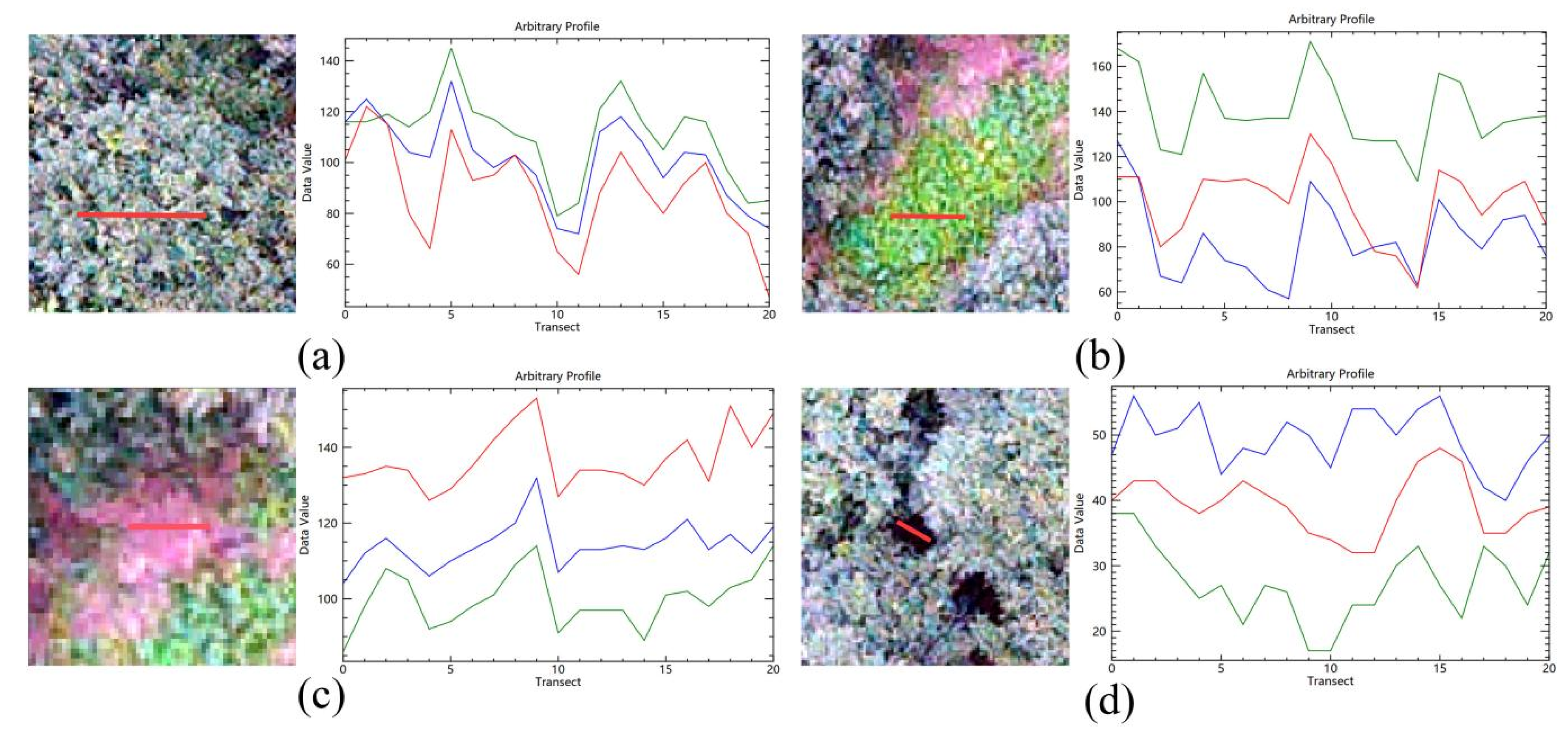
The spectral signatures of different land cover types form the basis for developing crown extraction methodologies. Spectral profiles of RGB bands were analyzed for four representative classes: C. oleifera crowns, weeds, bare soil, and forest gaps (Figure 4). Although both C. oleifera and weeds exhibit green vegetation characteristics, weed samples demonstrate significantly higher G-band values (110–170) compared with C. oleifera (80–145). Notably, C. oleifera exhibits relatively balanced RGB values, whereas weeds show marked dominance of the G band over the R (60–130) and B (55–125) bands. Forest gaps exhibit uniformly low RGB values, with the B band (40–57) being the highest. Bare soil shows pronounced variability in RGB values, particularly elevated R-band intensities (125–155).
Based on the collected sample data, the mean and standard deviation of RGB spectral values for four feature types were calculated, along with the CV, CRD (Table 4). All features exhibited low CV values (<50%) in the RGB bands, suggesting that these bands are conducive to clustering. The CRD between C. oleifera and other features was high (>100%), specifically with bare soil and forest gaps in the R band, with weeds and forest gaps in the G band, and notably with forest gaps in the B band.
To further evaluate the separability among different features in the visible-light bands, the J-M distances between C. oleifera and three types of background features were calculated. The J-M distance with bare soil was 1.88, indicating good separability, while those with weeds and forest gaps were 1.22 and 1.74, respectively, both below the 1.8 threshold. These results demonstrate that although some differences exist between C. oleifera and weeds/forest gaps in RGB bands, their separability is limited, and additional features are needed to improve discrimination.

3.2. Construction of the Image Feature Space

3.2.1. Vegetation Indices

Three visible-band vegetation indices were calculated for the study plots (Figure 5), and the CV, CRD of these indices for discriminating C. oleifera from background features were further computed using the samples data (Table 5).
The vegetation indices demonstrated more pronounced discriminative power between the C. oleifera canopy and background features than the RGB bands, with all CRDs exceeding 100% and the highest even surpassing 700%. However, the CV of the vegetation indices also increased accordingly, which may impede feature clustering. This suggests that RGB and three vegetation indices possess a certain degree of complementarity.
Using a feature space combining RGB bands with the MExG, VDVI, and NGBDI indices, the J-M distances between C. oleifera and bare soil, weeds, and forest gaps were 1.96, 1.73, and 1.96, respectively. These represent improvements of 4.26%, 41.80%, and 12.64% over using RGB features alone, confirming that incorporating vegetation indices enhances separability. Although the separability between C. oleifera and weeds improved markedly, the J-M distance still remained below the threshold of 1.8.

3.2.2. Canopy Height Model

As detailed in Section 2.4.1, a DSM, DEM, and CHM were generated for the study area, with results for the four standard plots presented in Figure 6. The CHM demonstrated a robust capability to differentiate C. oleifera crowns from background features via height variations, despite significant topographic differences. This was particularly evident in plots with multimodal canopy structures, which showed clear stratification.
By incorporating the CHM to leverage the significant height differences, the separability between C. oleifera and all background features improved, with J-M distances rising to 1.99, 1.96, and 1.97 (increases of 1.53%, 13.29%, and 0.51%). This confirms that the combined feature space of RGB, vegetation indices, and CHM effectively distinguishes C. oleifera from bare soil, weeds, and forest gaps. Thereby, it provides a crucial technical pathway for achieving “precise crown extraction and background removal.”

3.3. Identification of Bare Soil/Weeds

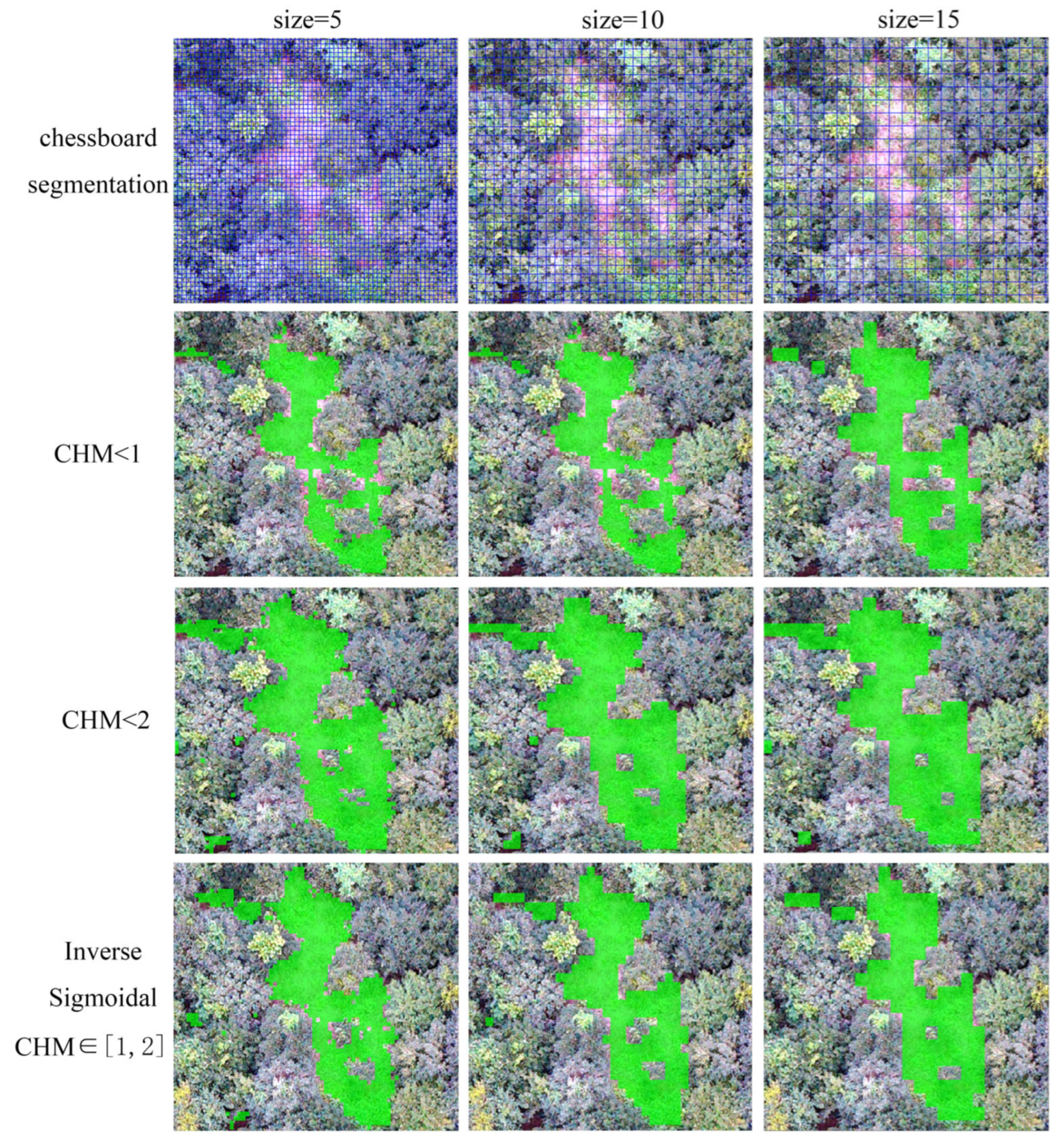
The first-level segmentation (chessboard segmentation) was performed to identify bare soil and weeds. Based on field survey data, the CHM served as a critical feature for distinguishing bare soil/weeds from C. oleifera canopies. Classification was performed on experimental areas H1 and L1 using CHM thresholds of <1 m and <2 m under-segmentation scales of 5, 10, and 15 pixels (top row, Figure 7). Rows 2 and 3 of Figure 7 provide a visual comparison of partial classification results, with accuracy assessed against reference data from visual interpretation (Table S5). Regardless of the size value, a high FN rate occurred in both experimental areas when the CHM was below 1 m, leading to low R. When the CHM threshold was increased to below 2 m, although missed detections were reduced, the commission error of weed areas increased, consequently resulting in lower P.
An Inverse Sigmoidal membership function was adopted for fuzzy classification of the imagery, with the discriminative interval of the CHM being defined as 1–2 m. When the CHM value of an object was below 1 m, its membership degree for the bare soil/weeds category approached 1; when it exceeded 2 m, the membership degree approached 0; within the 1–2 m range, the membership decreased smoothly with increasing height. The partial classification results are shown in row 4 of Figure 7.
The accuracy of fuzzy classification for identifying bare soil/weeds was evaluated at different segmentation scales using visually interpreted reference data. At Size = 5, undersized segments caused misclassification inside canopies and significant omissions in bare soil areas, yielding F-scores of 78.76% (H1) and 72.74% (L1). At Size = 15, oversized segments at edges contained mixed pixels, and high average CHM led to severe misclassification, reducing F-scores to 77.86% (H1) and 70.89% (L1). Size = 10 was optimal, preserving canopy integrity and restoring edge morphology, and achieved the highest F-scores (90.38% for H1, 87.10% for L1). These results provide a critical parametric basis for developing a dedicated segmentation algorithm suitable for high-closure canopies. Full-area results are shown in Figure S1.

3.4. Determination of Optimal Segmentation Parameters

3.4.1. Optimal Segmentation Scale

The ESP2 tool was utilized to preliminarily evaluate segmentation scales for different land cover types. The peaks in the rate of change (ROC) of image homogeneity curves indicate potential optimal scales for specific features (Figure 8). The ROC curve exhibits six distinct peaks (at scales 24, 31, 67, 79, 95, and 110), corresponding to optimal parameters for various land cover classes, with partial segmentation results shown in Figure S2. Scale 24 achieved superior segmentation for forest gaps, while scales 67 and 79 performed comparably for C. oleifera crown delineation. Conversely, scales 95 and 110 produce overly coarse results, failing to resolve individual tree crowns. Comparative analysis identified optimal parameters as scale 24 for forest gaps and scales 67/79 for C. oleifera crowns.

3.4.2. Parameterization for Forest Gap Segmentation

During the forest gap segmentation process, the scale parameter was set to 24, and shape/compactness were sequentially optimized using a single-variable approach. Initially, with the compactness fixed at 0.5, shape values from 0.1 to 0.9 were tested (Figure S3). Results showed that shape < 0.5 produced undersized segments, misclassifying dark canopy areas as gaps and causing severe fragmentation, while shape > 0.5 led to under-segmentation of darker gaps due to reduced spectral emphasis. A shape of 0.5 achieved the best boundary alignment with actual gaps.
Subsequently, with shape fixed at 0.5, compactness values from 0.1 to 0.9 were compared (Figure S4). Lower compactness (<0.5) resulted in redundant and complex edges, whereas higher compactness (>0.5) inadequately fitted small gap boundaries. Thus, the optimal parameters were determined as shape = 0.5 and compactness = 0.5. These parameters establish a critical foundation for the effective separation of C. oleifera tree crowns and forest gaps.

3.4.3. Parameterization for C. oleifera Segmentation

In the segmentation of C. oleifera canopies, this study evaluated the shape and compactness parameters at scale settings of 79 and 67. With the compactness fixed at 0.5, segmentation results with different shape values (0.1 to 0.9) were compared (Figures S5 and S6). Lower shape values (0.1, 0.3) caused overly flexible boundaries, leading to over segmentation of canopy shadows/gaps and fragmentation. Higher values (0.7, 0.9) resulted in oversmoothed contours that failed to capture actual edges, especially for small crowns. Shape = 0.5 achieved optimal balance between integrity and accuracy.
Subsequently, with the shape fixed at 0.5, compactness was further evaluated (Figures S7 and S8). Lower values (0.1, 0.3) produced complex, noisy edges, increasing background misclassification. Higher values (0.7, 0.9) created oversmoothed edges causing under-segmentation in adhered canopies. Compactness = 0.5 best balanced edge precision and morphological compactness. Thus, the optimal parameters were shape = 0.5 and compactness = 0.5. The selection of these parameters was critical for enabling precise individual tree segmentation in high-canopy-closure C. oleifera stands.

3.5. Nearest-Neighbor Classification with Multi-Feature Fusion

3.5.1. Feature Optimization and Frequency Statistics

To accurately identify C. oleifera canopies and forest gaps, this study conducted object-based image segmentation (OBIA) using the optimal parameters from Section 3.4.2 and selected classification samples based on the resulting segments.
The feature optimization algorithm in eCognition was employed to iteratively screen the initial 45 features. To strictly avoid overfitting and evaluate feature stability, a five-fold cross-validation framework was implemented. Representative samples from sites H1 and L1 were equally divided into five subsets. For each iteration, four subsets were used for feature optimization and one for validation. This process was repeated for five rounds per site, yielding ten optimized feature subsets.
A candidate feature set with high consistency and stability was constructed by selecting features with an occurrence frequency of no less than 50% across the ten subsets (Table 6). The final set contains 19 features, including seven with 100% frequency and five between 90% and 100%.

3.5.2. Feature Subset Evaluation and Generalization Validation

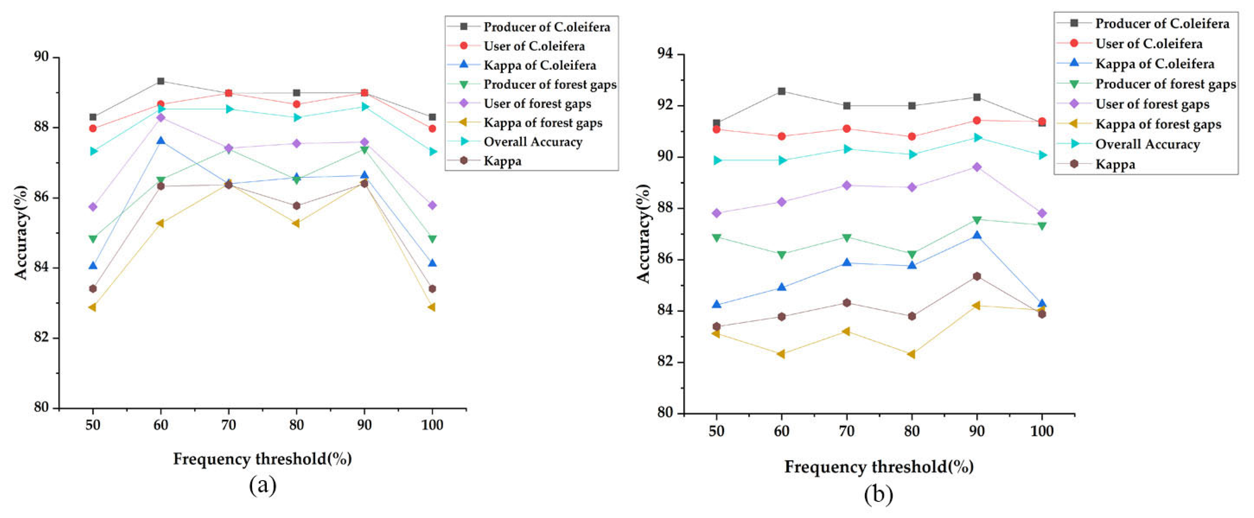
To evaluate the classification performance of different feature subsets, this study constructed multiple feature sets based on frequency thresholds ranging from 50% to 100%. Each subset was trained and evaluated using a nearest neighbor classifier in experimental sites H1 and L1, with mean classification accuracy shown in Figure 9.
The results indicate that all feature subsets achieved a high classification accuracy (Kappa > 0.8). Increasing the frequency thresholds reduced the feature numbers while causing fluctuating accuracy. At the 90% threshold, both the overall accuracy (OA) and Kappa coefficients reached their maximum values in H1 and L1 (H1: OA = 88.60%, Kappa = 86.41%; L1: OA = 90.76%, Kappa = 85.36%).
In H1, increasing the threshold from 50% to 60% reduced the features from 19 to 16, improving all accuracy metrics (OA +1.21%, Kappa +2.93%). Accuracy showed minor fluctuations at 60–90% thresholds but declined significantly at the 100% threshold (with seven features remaining). For L1, accuracy remained stable with slight improvements at the 50–90% thresholds, followed by a substantial decline at the 100% threshold.
Balancing classification performance and feature redundancy, 12 features at the 90% frequency threshold were selected as the optimal set. When applied to independent validation sites H2 and L2, this achieved an OA of 95.00% and 94.17%, with Kappa of 86.84% and 88.10%, respectively. The results demonstrate strong generalization capability for high-accuracy identification of C. oleifera canopies and forest gaps across mountainous areas at different elevations.

3.6. Accuracy Assessment of Canopy Identification Results

Comparative experiments using single-scale segmentation (optimal scales: 67 and 79) with nearest-neighbor classification in sites H1 and L1. Their F-scores reached 92.34% and 89.76% at scale = 67 and 93.24% and 89.29% at scale = 79. Despite these high values, significant misclassification occurred: commission errors reached 346.33 m2/370.29 m2 at scale 67 and increased to 502.01 m2/486.05 m2 at scale 79. This primarily resulted from the high canopy density where non-target features occupied small areas, but single-scale segmentation failed to accurately delineate boundaries, causing substantial misclassification.
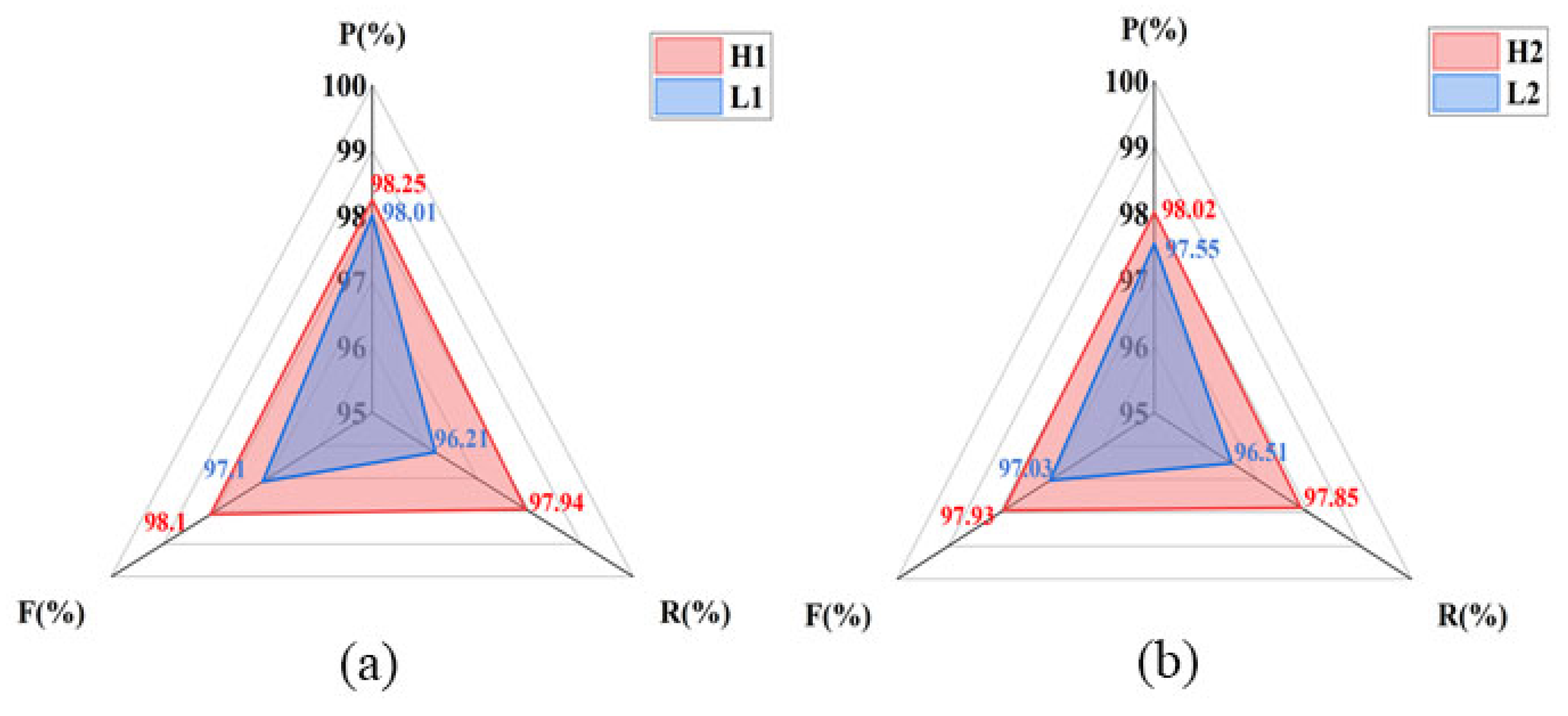
The canopy identification accuracy of the multi-level segmentation method was quantitatively evaluated (Figure 10). In H1 and L1 at different elevations, the F-scores for C. oleifera canopy recognition reached 98.10% and 97.10%, respectively, representing improvements of at least 4.86% and 7.34% over single-scale methods. Commission errors were reduced by ≥290.90 m2 and ≥428.09 m2, and omission errors decreased by ≥14.53 m2 and ≥30.25 m2. In independent validation sites H2 and L2, the average F-score remained high at 97.48%. These results demonstrate that the strategy of initially eliminating background interference (bare soil/weeds, gaps) followed by refined canopy extraction significantly improves recognition accuracy in dense, complex environments, effectively minimizing both commission and omission errors.

3.7. Object-Oriented Crown Segmentation

3.7.1. Single-Level Crown Segmentation

Building upon Section 3.6, a third-level segmentation was implemented to achieve individual crown delineation. Using the optimal parameters from Section 3.4.3, single-level segmentation achieved F-scores of 72.97% and 75.49% (scale = 67), 68.22% and 77.39% (scale = 79) in H1 and L1. Although single-level segmentation identified most canopies, significant under-segmentation persisted where single patches contained multiple crowns, resulting in low individual tree detection accuracy. The issue stems from variations in canopy connectivity within the same region, where clustered canopies form large patches. This necessitates a hierarchical approach to optimize the under-segmented large patch areas.

3.7.2. Multi-Level Segmentation Strategy and Accuracy Improvement

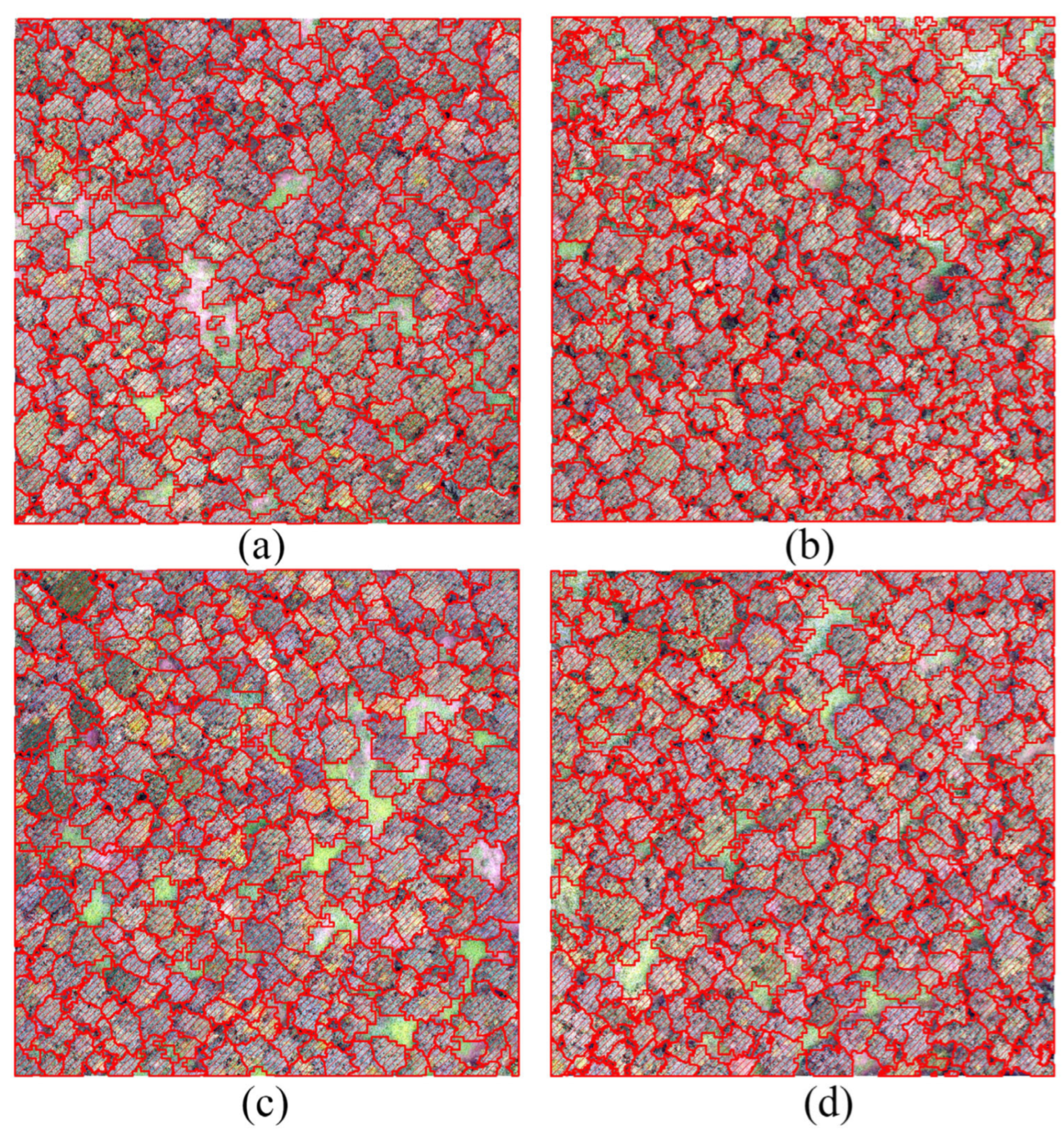
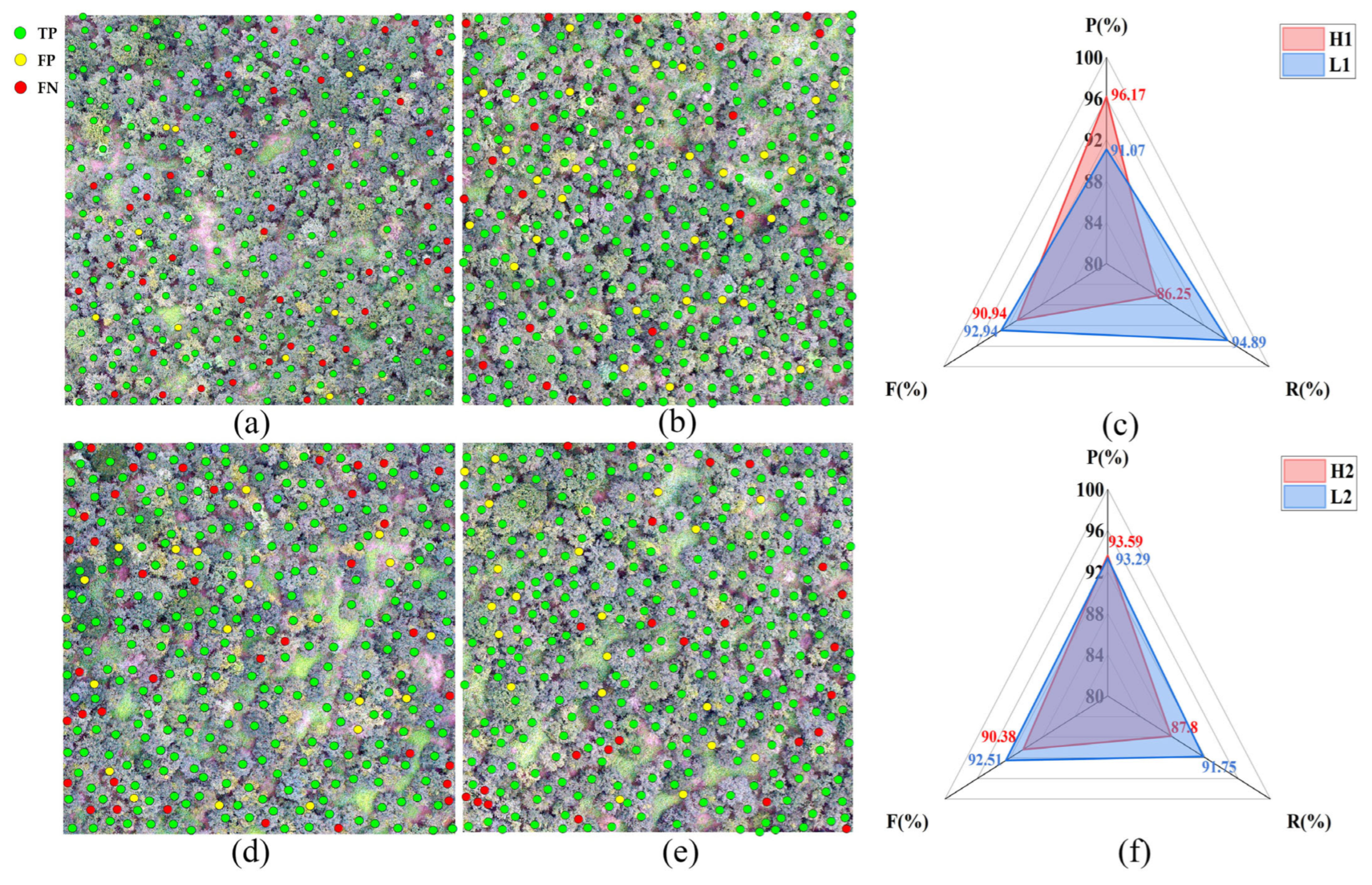
This study adopted a hierarchical segmentation strategy to leverage multi-scale advantages; an initial segmentation at scale = 79 captured macro-level canopy clusters, preserving overall structure and spatial context. To address under-segmentation in large patches, a region-specific statistical framework was developed using Formula (8) and Table 7 parameters to construct multi-level structures for H1 and L1. Subsequently, under-segmented patches were refined at scale = 67 to resolve individual crowns in dense areas, effectively balancing global integrity and local accuracy in high-density forests (Figure 11). The tree identification results are illustrated in Figure 12.
The results demonstrated significant accuracy improvements. F-scores exceeded 90% in both H1 and L1, with P, R, and F increasing by 6.37%, 30.02%, and 21.78% in H1, and 6.09%, 17.59%, and 12.73% in L1. Validation in independent sites H2 and L2 achieved F-scores of 92.94% and 91.69%, respectively. The average metrics across all four sites reached 93.53% (P), 90.07% (R), and 91.69% (F), confirming the method’s robustness and stability in mountainous terrain and high-canopy-density environments.

3.8. Extraction and Validation of Tree Height and Crown Width Parameters

(1)
Tree Height Extraction
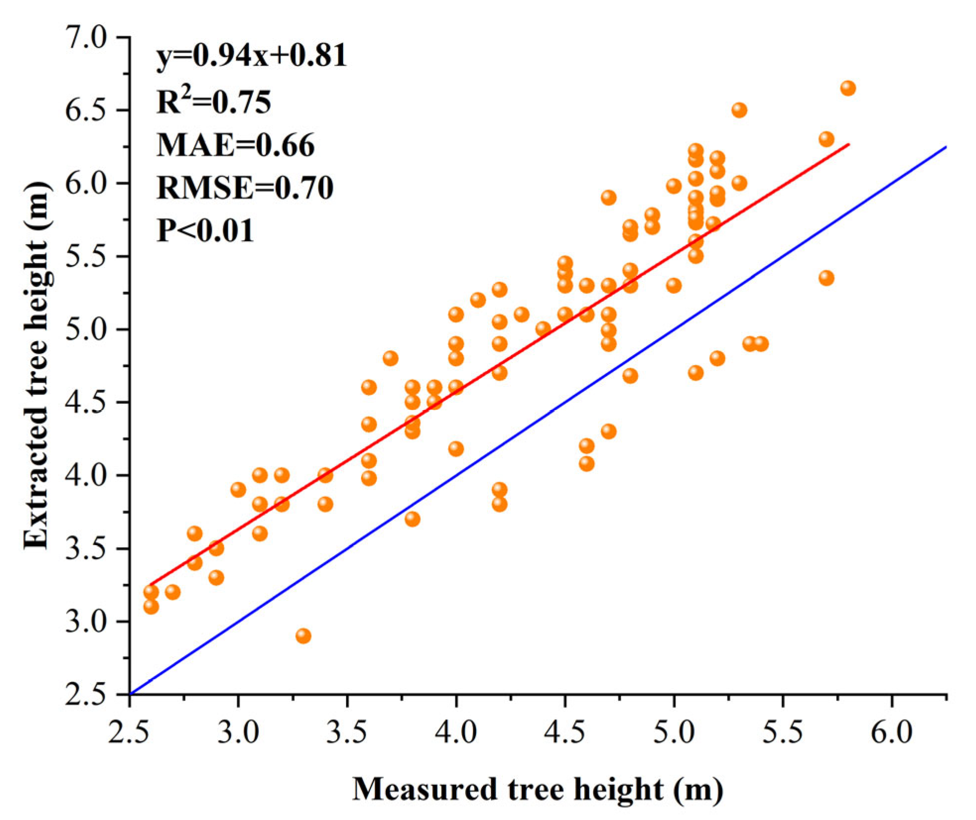
Tree heights were derived by extracting the maximum CHM value within each segmented crown polygon using ArcGIS Pro 3.0.2 Field-surveyed tree height measurements (n = 100) served as ground-truth references for validation. After excluding outliers with significant discrepancies, linear regression analysis was performed between LiDAR-derived tree heights and field measurements, and the results are illustrated in Figure 13. The extracted tree heights showed strong agreement with field measurements (R2 = 0.75). This result confirms that our integrated method—fusing LiDAR and visible-light imagery within a hierarchical segmentation process—enables precise crown extraction and ensures accurate estimation of tree structural parameters.
(2)
Crown Width Parameter Extraction
Linear regression analysis was performed between field-measured crown dimensions (n = 96, excluding four outliers) and multi-level crown-segmentation-derived values (Figure 14). The east–west and south–north crown width fittings both achieved R2 above 0.6, while the mean crown width model yielded the best result (R2 = 0.75). The results demonstrate that the proposed multi-level segmentation method maintains reliable structural parameter extraction accuracy even under challenging illumination conditions, validating the robustness and applicability of the developed dedicated segmentation algorithm in high-closure canopies.
(3)
Impact of Segmentation Errors on Forest Parameter Estimation
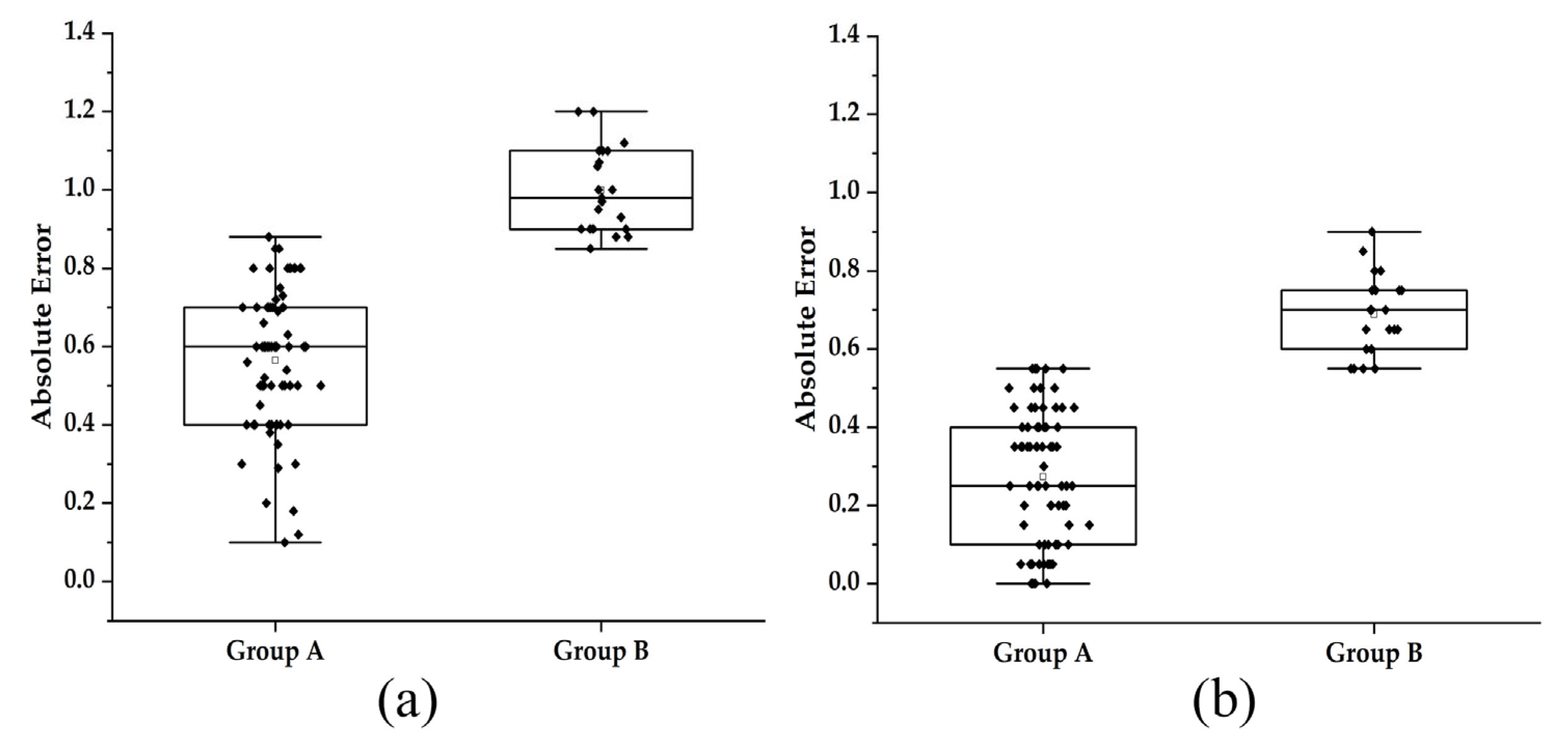
To quantify the impact of segmentation quality on the accuracy of subsequent parameter extraction, this study divided 96 validation samples (after removing outliers) into two groups based on visual interpretation: Group A (well segmented, n = 75), where segmentation polygons closely matched the true crown outlines, and Group B (poorly segmented, n = 21), which included samples with significant errors (FP and FN). The extraction errors for tree height and crown diameter were calculated for each group (Table 8), and the distributions of absolute errors were visualized using boxplots (Figure 15).
Analysis of tree height and crown width extraction errors demonstrates that segmentation quality directly determines parameter estimation accuracy. Figure 5 revealed consistently lower error distributions in Group A than Group B: tree height errors concentrated at 0.40–0.70 m in Group A versus 0.9–1.1 m in Group B, while crown width errors ranged 0.1–0.4 m in Group A compared to 0.6–0.8 m in Group B. Major errors in Group B consistently corresponded to severe segmentation failures (including FN and FP), confirming that inaccuracies introduced during segmentation constitute the primary source of uncertainty in parameter estimation. This finding underscores the critical importance of segmentation precision for ensuring reliable tree parameter extraction, validating both the necessity and effectiveness of developing a dedicated segmentation algorithm for high-closure environments.

4. Discussion

4.1. Effectiveness and Adaptability of the Method in Mountainous Environments

(1)
Effectiveness of Background Removal and Parameter Sensitivity
Accurate delineation of dense tree canopies from complex understory backgrounds remains a typical challenge in forestry remote sensing within mountainous regions. Based on preliminary findings (Table S5) showing high FN rates when the CHM was below 1 m and increased FP when the threshold was raised to 2 m, a smooth transition zone of 1–2 m was established. To address the limitations of hard-threshold methods, which struggle with continuous elevation variations and classification ambiguities in hilly terrain [12], this study proposes a fuzzy classification strategy that integrates chessboard segmentation with a transitional CHM zone (1–2 m). By explicitly modeling classification uncertainty, our method overcomes key limitations of hard-threshold approaches in complex environments (Figure 5). This aligns with probabilistic classification trends in forestry remote sensing [52] and is specifically tailored for high-closure C. oleifera plantations. Experimental results show significant reductions in both FP and FN rates, demonstrating robust performance under challenging conditions. Our method’s sensitivity to the “Size” parameter aligns with OBIA studies in heterogeneous landscapes [19,20]. Sensitivity analysis shows the optimal value (10 pixels) closely corresponds to the characteristic scale of bare soil and weed patches in our mountainous study area. This supports the view that segmentation parameters require calibration to specific forest structures [53]. Future work should investigate automated parameter optimization to improve transferability.
(2)
Effectiveness of Multi-Feature Fusion and Optimization for Object Separation
The challenge of distinguishing spectrally similar objects in mountainous terrain underscores a fundamental limitation of single-feature approaches in remote sensing. While the utility of multi-source data fusion is conceptually well-established in the literature [54], our study provides an empirical, hierarchical validation of its mechanics: RGB data initiates a basic separation, vegetation indices (MExG, VDVI, NGBDI) amplify spectral discriminability, and the CHM introduces a critical structural dimension to resolve residual ambiguities. This step-wise framework moves beyond the established principle and offers a replicable project for feature engineering in analogous complex environments.
The optimized 12-feature subset developed for forest gap removal demonstrates a critical refinement in feature engineering for complex environments. Addressing the common issues of redundancy and instability in multi-feature fusion [55], we employed a 90% frequency threshold for feature selection, advancing multi-source feature fusion from simple feature stacking to precise feature refinement. This method achieved an overall accuracy of 92.13% in both experimental and validation areas, confirming not only the strategy’s effectiveness but also establishing a robust and generalizable model. This provides a practical and feasible solution for precise segmentation in complex mountainous regions.

4.2. Advantages of Multi-Level Segmentation for High-Canopy-Closure Stands

To address the challenge of crown adhesion in high-canopy-closure forests, we propose a “coarse-to-fine” multi-level segmentation strategy. Traditional single-level segmentation methods often lead to severe under-segmentation in such environments, whereas our hierarchical framework effectively resolves this scale-related issue. By first removing background noise and then performing targeted secondary segmentation on initially under-segmented areas, our approach implements the principle that “a single optimal scale is not suitable for all objects” [53]. The final F-score increased from 73.52% to 91.69%, surpassing the accuracy reported in some high-density forest studies [5]. This demonstrates not only an improvement in accuracy but also validates a conceptual shift from a single segmentation model to an adaptive process-oriented model, providing a new paradigm for effectively resolving the crown adhesion problem.

4.3. Accuracy Limitations and Error Sources

Although the method performs well in canopy extraction and individual tree identification, its accuracy in precise crown delineation (R2 < 0.8, Figure 14) reflects a common challenge across segmentation techniques. Errors primarily arise from three sources: under-segmentation in dense canopy areas (Table 8, Figure 15), geometric approximation errors during polygon-to-width conversion, and field measurement subjectivity under complex canopy structures. These systematic discrepancies collectively underscore a fundamental tension between model abstraction and biological reality. Our results substantiate the findings of Xie et al. [54], confirming that even robust segmentation methods remain constrained by forest structural complexity. This convergence of evidence highlights that achieving high morphological accuracy requires not only algorithmic refinement but also a critical understanding of the ecological context in which these techniques are deployed.

4.4. Limitations and Future Work

The proposed method proves effective in mountainous C. oleifera forests, yet its limitations highlight critical challenges in forestry remote sensing. Its reliance on significant canopy-background height difference reflects a known constraint in LiDAR-based segmentation, particularly in high-closure canopies where limited penetration and reduced contrast affect performance. Furthermore, while parameters were optimized for our study area, their fixed nature highlights a pervasive scalability issue in heterogeneous environments.
To advance beyond these constraints, future research should pursue two synergistic paths: developing dynamically adaptive parameters responsive to local terrain and canopy structure [55], and creating multi-feature fusion strategies robust to minimal height variations [56]. Notably, integrating this study’s physical rules with lightweight deep learning architectures [57] presents a promising hybrid pathway, potentially balancing the interpretability of process-based models with the representational power of data-driven approaches. Although 3D canopy modeling offers theoretical advantages for crown delineation [58], its computational demands currently constrain operational scalability. We therefore advocate for strategic development of lightweight morphological algorithms that maintain the accuracy-efficiency balance is essential for large-scale forestry applications.

5. Conclusions

This study presents a novel multi-level segmentation method for precisely extracting individual tree crowns in mountainous C. oleifera plantations under high canopy closure, using integrated UAV imagery and LiDAR data. We developed an object-based hierarchical segmentation process by fusing multi-source features from optical and point cloud data, enabling accurate crown extraction and effective background removal. Furthermore, a dedicated coarse-to-fine segmentation strategy was designed for dense canopy conditions, which substantially improved the segmentation performance—raising the F-score of individual tree detection from 73.52% to 91.69%. Experimental results demonstrated that our method achieved an F-score of 97.54% in canopy coverage extraction, along with R2 values of 0.75 for both tree height and crown width estimation, confirming its high accuracy and practical utility. This work not only provides a reliable technical solution for the precision monitoring of C. oleifera plantations, but also offers a valuable reference for parameter extraction in other economically important tree species. Future research will focus on developing adaptive parameters and exploring hybrid strategies that combine physical rules with lightweight deep learning architectures.

Supplementary Materials

The following supporting information can be downloaded at: https://www.mdpi.com/article/10.3390/agronomy15112522/s1, Table S1: Sensor specifications; Table S2: Hi-POS inertial navigation system IMU performance specifications; Table S3: Technical specification of UAV flight campaigns; Table S4: Formulas and descriptions for CV and CRD; Table S5: Accuracy assessment of bare soil/weed classification under different segmentation scales and CHM thresholds in experimental area H1; Figure S1: Identification results for bare soil/weeds in the H1 (a) and L1 (b) experimental areas; Figure S2: Comparison of scale parameters for segmenting C. oleifera crowns; Figure S3: Comparative analysis of segmentation results under different shape values for forest gap (Scale=24, Compactness=0.5); Figure S4: Comparative analysis of segmentation results under different compactness values for forest gap (Scale=24, Shape=0.5); Figure S5: Comparative analysis of segmentation results under different shape values for C. oleifera (scale=79, compactness=0.5); Figure S6: Comparative analysis of segmentation results under different shape values for C. oleifera (scale=67, compactness=0.5); Figure S7: Comparative analysis of segmentation results under different compactness values for C. oleifera (scale=79, shape=0.5); Figure S8: Comparative analysis of segmentation results under different compactness values for C. oleifera (scale=67, shape=0.5).

Author Contributions

Conceptualization, S.L., J.Z. and D.M.; methodology, S.L. and Z.L.; software, Z.L. and J.L.; validation, S.L. and Z.L.; investigation, S.L.; resources, Y.W.; data curation, J.L. and J.Z.; writing—original draft preparation, S.L. and Z.L.; writing—review and editing, S.L., J.Z. and D.M.; funding acquisition, S.L. and Y.W. All authors have read and agreed to the published version of the manuscript.

Funding

This research was funded by the 2024 Annual Research Project of Guangxi Philosophy and Social Sciences (24GLC002), the Project of Guangxi Key Research and Development Program (GuikeAB25069153), and the Project of Guangxi Key Research and Development Program (GuikeAB25069412).

Data Availability Statement

The data presented in this study are available from the corresponding author upon request.

Acknowledgments

We sincerely thank Hailin Ming, Peilin Li, Xiaoye Chen, Chuzhao Li, Wenqi Liu, Yan Liu, and Qinyu Huang from the School of Natural Resources and Surveying, Nanning Normal University, and we thank Fei Cheng, Bowen Dong, and Rongao Zhang from the College of Forestry, Guangxi University, for their various types of assistance in field sampling for this study. We sincerely thank the Nanning Branch of Guangzhou Hi-Target Navigation Technology Co., Ltd. for providing the UAV and sensor equipment and for their assistance in acquiring UAV data for our research area.

Conflicts of Interest

Jie Zhang was employed by the Guangxi Environmental Protection Industry Investment Group Co., Ltd. The remaining authors declare that the research was conducted in the absence of any commercial or financial relationships that could be construed as a potential conflict of interest.

References

  1. He, X.S.; Zhou, W.C.; Qiu, F.Y.; Gong, C.; Xu, L.C.; Xiao, X.X.; Wang, Y.J. Responses of different Camellia oleifera varieties to drought stress and the comprehensive evaluation of their drought resistance. J. Cent. South Univ. For. Technol. 2023, 43, 1–14. [Google Scholar]
  2. Zhang, D.S.; Jin, Q.Z.; Xue, Y.L.; Zhang, D.; Wang, X.G. Nutritional value and adulteration identification of oil-tea Camellia seed oil. China Oils Fats 2013, 38, 47–50. [Google Scholar]
  3. National Forestry and Grassland Administration National Park Administration. Available online: https://www.forestry.gov.cn/lyj/1/ggjjlcy/20250422/622027.html (accessed on 10 September 2025).
  4. The People’s Government of Guangxi Zhuang Autonomous Region. Available online: http://www.gxzf.gov.cn/mlgxi/gxrw/zrdl/t20886294.shtml (accessed on 10 September 2025).
  5. Zhou, X.C.; Wang, P.; Tan, F.L.; Chen, C.C.; Huang, H.Y.; Lin, Y. Biomass estimation of high-density forest harvesting based on Multi-temporal UAV Images. Trans. Chin. Soc. Agric. Mach. 2023, 54, 168–177. [Google Scholar]
  6. He, B.K.; Zhu, W.Q.; Shi, P.J.; Zhang, H.; Liu, R.Y.; Yang, X.Y.; Zhao, C.L. A Fine-Scale Remote Sensing Estimation Method for Fractional Vegetation Cover in Complex Terrain Areas: A Case Study in the Qinghai-Tibet Plateau Mountainous Regions. Acta Ecol. Sin. 2024, 44, 9039–9052. [Google Scholar]
  7. Zhang, H.L.; Wang, Y.; Hu, M.; Zhang, Y.Z.; Zhang, J.; Zhan, B.S.; Liu, X.M.; Luo, W. Application of multispectral index features based on sigmoid function normalization in remote sensing identification and sample migration study of Camellia oleifera Forest. Spectrosc. Spectr. Anal. 2025, 45, 1159–1167. [Google Scholar]
  8. Chen, Z.J.; Cheng, G.; Pu, Y.K.; Huang, W.; Chen, J.H.; Li, W.Z. Single tree parameters extraction of broad-leaved forest based on UAV tilting photography. For. Resour. Manag. 2022, 1, 132–141. [Google Scholar]
  9. Li, R.; Sun, Z.; Xie, Y.H.; Li, W.H.; Zhang, Y.L.; Sun, Y.J. Extraction of tree crown parameters of high-density pure Cunninghamia lanceolata plantations by combining the U-net model and watershed algorithm. Chin. J. Appl. Ecol. 2023, 34, 1024–1034. [Google Scholar]
  10. Pourreza, M.; Moradi, F.; Khosravi, M.; Deljouei, A.; Vanderhoof, M.K. GCPs-free photogrammetry for estimating tree height and crown diameter in Arizona Cypress plantation using UAV-Mounted GNSS RTK. Forests 2022, 13, 1905. [Google Scholar] [CrossRef]
  11. Panagiotidis, D.; Abdollahnejad, A.; Peter, S.; Chiteculo, V. Determining tree height and crown diameter from high-resolution UAV imagery. Int. J. Remote Sen. 2017, 38, 2392–2410. [Google Scholar] [CrossRef]
  12. Wu, Y.D.; Han, H. Extraction of forest canopy height and width using UAV aerial survey data in the Gannan Plateau. J. Gansu Agric. Univ. 2024, 59, 268–276. [Google Scholar]
  13. Wang, J.; Zhang, C.; Chen, Q.; Li, Y.H.; Peng, X.; Bai, M.X.; Xu, Z.Y.; Liu, H.D.; Chen, Y.F. The method of extracting information of Cunninghamia lanceolata crown combined with RGB and LiDAR based on UAV. J. Southwest For. Univ. 2022, 42, 133–141. [Google Scholar]
  14. Jin, Z.M.; Cao, S.S.; Wang, L.; Sun, W. A method for individual tree-crown extraction from UAV remote sensing image based on U-net and water shed algorithm. J. Northwest For. Univ. 2020, 35, 194–204. [Google Scholar]
  15. Li, Y.D.; Cao, M.L.; Li, C.Q.; Feng, Z.K.; Jia, S.H. Crown segmentation from UAV visible light DOM based on level set method. Trans. Chin. Soc. Agric. Eng. 2021, 37, 60–65. [Google Scholar]
  16. Bai, M.X.; Zhang, C.; Chen, Q.; Wang, J.; Li, Y.H.; Shi, X.R.; Tian, X.Y.; Zhang, Y.W. Study on the extraction of individual tree height based on UAV visual spectrum remote sensing. For. Resour. Manag. 2021, 1, 164–172. [Google Scholar]
  17. Wang, W.Y.; Li, F.; Hasituya; Hashengaowa. Information extraction of agricultural greenhouses types based on object-oriented multi-level multi-scale segmentation. J. China Agric. Univ. 2024, 29, 223–236. [Google Scholar]
  18. Li, X.C.; Long, J.P. Research on UAV Image Enhancement Based on Visible Light Vegetation Index. Cent. South For. Inventory Plan. 2024, 43, 38–43. [Google Scholar]
  19. Gao, F.; Shi, H.J.; Shui, J.F.; Zhang, Y.; Guo, M.H.; Wen, Z.M. Structural parameter extraction of artificial forest in northern Shaanxi based on UAV high-resolution image. Sci. Soil Water Conserv. 2021, 19, 1–12. [Google Scholar]
  20. Wu, N.S.; Wang, J.X.; Zhang, Y.; Yuan, M.T.; Zhang, Q.; Gao, C.Y. Determining tree species and crown width from unmanned aerial vehicle imagery in hilly loess region of west Shanxi, China: A case study from Caijiachuan watershed. Acta Agric. Zhejiangensis 2021, 33, 1505–1518. [Google Scholar]
  21. Li, L.; Mu, X.; Chianucci, F.; Qi, J.; Jiang, J.; Zhou, J.; Chen, L.; Huang, H.; Yan, G.; Liu, S. Ultrahigh-resolution boreal forest canopy mapping: Combining UAV imagery and photogrammetric point clouds in a deep-learning-based approach. Int. J. Appl. Earth Obs. 2022, 107, 102686. [Google Scholar] [CrossRef]
  22. Ferro, M.V.; Srensen, C.G.; Catania, P. Comparison of different computer vision methods for vineyard canopy detection using UAV multispectral images. Comput. Electron. Agric. 2024, 225, 109277. [Google Scholar] [CrossRef]
  23. Hao, Z.; Lin, L.; Post, C.J.; Mikhailova, E.A.; Li, M.; Chen, Y.; Yu, K.; Liu, J. Automated tree-crown and height detection in a young forest plantation using mask region-based convolutional neural network (Mask R-CNN). ISPRS J. Photogramm. 2021, 178, 112–123. [Google Scholar] [CrossRef]
  24. Puletti, N.; Guasti, M.; Innocenti, S.; Cesaretti, L.; Chiavetta, U. A semi-automatic approach for tree crown competition indices assessment from UAV LiDAR. Remote Sens. 2024, 16, 2576. [Google Scholar] [CrossRef]
  25. Zhu, B.D.; Luo, H.B.; Jin, J.; Yue, C.R. Optimization of Individual Tree Segmentation Methods for High Canopy Density Plantation Based on UAV LiDAR. Sci. Silvae Sin. 2022, 58, 48–59. [Google Scholar]
  26. Li, P.H.; Shen, X.; Dai, J.S.; Cao, L. Comparisons and Accuracy Assessments of LiDAR-Based Tree Segmentation Approaches in Planted Forests. Sci. Silvae Sin. 2018, 54, 127–136. [Google Scholar]
  27. Fu, Y.; Niu, Y.; Wang, L.; Li, W. Individual-tree segmentation from UAV–LiDAR data using a region-growing segmentation and supervoxel-weighted fuzzy clustering approach. Remote Sens. 2024, 16, 608. [Google Scholar] [CrossRef]
  28. Quan, Y.; Li, M.; Zhen, Z.; Hao, Y.; Wang, B. The feasibility of modelling the crown profile of Larix olgensis using Unmanned Aerial Vehicle laser scanning data. Sensors 2020, 20, 5555. [Google Scholar] [CrossRef] [PubMed]
  29. Wei, X.B.; Li, Z.Q.; Chen, S.G.; Liu, R. Single tree segmentation of mangrove trees of different species based on UAV-LiDAR. Sci. Technol. Eng. 2024, 24, 963–969. [Google Scholar]
  30. Wang, X.Y.; Huang, Y.; Xing, Y.Q.; Li, D.J.; Zhao, X.W. The single tree segmentation of UAV high-density LiDAR point cloud data based on coniferous plantations. J. Cent. South Univ. For. Technol. 2022, 42, 66–77. [Google Scholar]
  31. Huang, B.Q.; Cao, B.; Yue, C.R.; Zhou, Q. Research on a method for individual tree segmentation for mountains coniferous forests using UAV-LiDAR technology. Cent. South For. Inventory Plan. 2024, 43, 34–39+48. [Google Scholar]
  32. Li, H.K.; Wang, J.; Zhou, Y.B.; Long, B.P. Extraction of Camellia oleifera planting areas in southern hilly area by combining multi-features of time-series Sentinel data. Trans. Chin. Soc. Agric. Mach. 2024, 55, 241–251. [Google Scholar]
  33. Meng, H.R.; Li, C.J.; Zheng, X.Y.; Gong, Y.S.; Liu, Y.; Pan, Y.C. Research on extraction Camellia oleifera by integrating spectral, texture and time sequence remote sensing information. Spectrosc. Spectr. Anal. 2023, 43, 1589–1597. [Google Scholar]
  34. Gao, X.X.; Wang, T.H.; Chen, L.S.; Liu, S.H.; Shuai, X.Q.; Xie, A. Study on remote sensing extracting Camellia oleifera forest based on GF-6 multispectral imagery. Guizhou Agric. Sci. 2024, 52, 117–125. [Google Scholar]
  35. He, C.R.; Fan, Y.L.; Tan, B.X.; Yu, H.; Shen, M.T.; Huang, Y.F. Extraction and identification of Camellia oleifera plantations based on multi-feature combination of “Zhuhai-1” satellite images. J. Northwest For. Univ. 2024, 39, 61–70. [Google Scholar]
  36. Liu, J.Y.; Gao, Z.C.; Liu, H.Y.; Yin, J.Q.; Luo, Y.Y. Research on sorting task of Camellia oleifera fruit based on YOLOv8 improved algorithm. J. For. Eng. 2025, 10, 120–127. [Google Scholar]
  37. Xiao, S.P.; Zhao, Q.Y.; Zeng, J.Y.; Peng, Z.R. Camellia oleifera fruits occlusion detection and counting in complex environments based on improved YOLO–DCL. Trans. Chin. Soc. Agric. Mach. 2024, 55, 318–326+480. [Google Scholar]
  38. Li, Q.S.; Kang, L.C.; Yao, H.H.; Li, Z.F.; Liu, M.H. Recognition method of Camellia oleifera fruit in natural environment based on improved YOLOv4–Tiny. J. Chin. Agric. Mech. 2023, 44, 224–230. [Google Scholar]
  39. Yin, X.M.; Peng, S.F.; Cheng, J.Y.; Chen, Q.M.; Zhang, R.Q.; Mo, D.K.; Wei, W.; Yan, E.P. Identification of Camellia osmantha fruit based on deep learning. Non-Wood For. Res. 2023, 41, 70–81. [Google Scholar]
  40. Chen, F.J.; Chen, C.; Zhu, X.Y.; Shen, D.Y.; Zhang, X.W. Detection of Camellia oleifera fruit maturity based on improved YOLOv7. Trans. Chin. Soc. Agric. Eng. 2024, 40, 177–186. [Google Scholar]
  41. Yu, J.; Yan, E.; Yin, X.; Song, Y.; Wei, W.; Mo, D. Automated extraction of Camellia oleifera crown using unmanned aerial vehicle visible images and the ResU-Net deep learning model. Front. Plant Sci. 2022, 13, 958940. [Google Scholar]
  42. Wu, J.; Peng, S.F.; Jiang, F.G.; Tang, J.; Sun, H. Extraction of Camellia oleifera crown width based on the method of optimized watershed with multi-scale markers. Chin. J. Appl. Ecol. 2021, 32, 2449–2457. [Google Scholar]
  43. Gao, S.; Yuan, X.P.; Gan, S.; Yang, Y.F.; Li, X. Application of airborne LiDAR and UAV image fusion for complicated terrain. Bull. Surv. Mapp. 2021, 7, 65–69. [Google Scholar]
  44. Hu, Z.Y.; Shan, L.; Chen, X.Y.; Yu, K.Y.; Liu, J. Individual Tree Segmentation of UAV-LiDAR Based on the Combination of CHM and DSM. Sci. Silvae Sin. 2024, 60, 14–24. [Google Scholar]
  45. Sun, G.X.; Li, Y.B.; Wang, X.C.; Hu, G.Y.; Zhang, Y. Image segmentation algorithm for greenhouse cucumber canopy under various natural lighting conditions. Int. J. Agr. Bio. Eng. 2016, 9, 130–138. [Google Scholar]
  46. Wang, X.Q.; Wang, M.M.; Wang, S.Q.; Wu, Y.D. Extraction of vegetation information from visible unmanned aerial vehicle images. Trans. Chin. Soc. Agric. Eng. 2015, 31, 152–159. [Google Scholar]
  47. Li, P.F.; Guo, X.P.; Gu, Q.M.; Zhang, X.; Feng, C.D.; Guo, G. Vegetation coverage information extraction of mine dump slope in Wuhai City of Inner Mongolia based on visible vegetation index. J. Beijing For. Univ. 2020, 42, 102–112. [Google Scholar]
  48. Zong, H.L.; Yuan, X.P.; Gan, S.; Yang, M.L.; Lv, J.; Zhang, X.L. Spatial Distribution Mapping of Debris Flow Site in Xiaojiang River Basin Based on the GEE Platform. Spectrosc. Spectr. Anal. 2025, 45, 1045–1060. [Google Scholar]
  49. Zheng, X.; Qiu, C.X.; Li, C.J.; Zhou, J.P.; Huai, H.J.; Wang, J.Y.; Zhang, Q.Y. Object-oriented subfield boundary extraction from UAV remote sensing images. Sci. Technol. Innov. 2022, 3, 1–3. [Google Scholar]
  50. Goutte, C.; Gaussier, E. A probabilistic interpretation of precision, recall and F-score, with implication for evaluation. In Advances in Information Retrieval; Lecture Notes in Computer Science; Springer: Berlin/Heidelberg, Germany, 2005; p. 952. [Google Scholar]
  51. Sokolova, M.; Japkowicz, N.; Szpakowicz, S. Beyond accuracy, F-score and ROC: A family of discriminant measures for performance evaluation. In AI 2006: Advances in Artificial Intelligence; Lecture Notes in Computer Science; Springer: Berlin/Heidelberg, Germany, 2006; pp. 1015–1021. [Google Scholar]
  52. Zheng, M.; Bao, Y.Y.; Li, J.X.; Li, X.L.; Wang, L.; Zhang, J. Research and application of identification of patchily degraded alpine meadows based on UAV imagery. Acta Ecol. Sin. 2026, 1, 1–15, Online First. [Google Scholar]
  53. Sun, Z.; Pan, L.; Sun, Y.J. Extraction of tree crown parameters from high-density pure Chinese fir plantations based on UAV image. J. Beijing For. Univ. 2020, 42, 20–26. [Google Scholar]
  54. Xie, Y.H.; Jing, X.H.; Sun, Z.; Ding, Z.D.; Li, R.; Li, H.W.; Sun, Y.J. Tree crown extraction of UAV remote sensing high canopy density stand based on instance segmentation. For. Res. 2022, 35, 14–21. [Google Scholar]
  55. Yan, P.F.; Ming, D.P. Segmentation of high spatial resolution remotely sensed data using watershed with self-adaptive parameterization. Remote Sens. Technol. Appl. 2018, 33, 321–330. [Google Scholar]
  56. Quan, Y.; Li, M.Z.; Zhen, Z.; Hao, Y.S. Modeling crown characteristic attributes and profile of Larix olgensis using UAV-borne LiDAR. J. Northeast For. Univ. 2019, 47, 52–58. [Google Scholar]
  57. Harders, L.O.; Ufer, T.; Wrede, A.; Hussmann, S.H. UAV-based real-time weed detection in horticulture using edge processing. J. Electron. Imaging 2023, 32, 052405. [Google Scholar] [CrossRef]
  58. Long, K.Y.; Long, J.P.; Lin, H.; Sun, H.; Xu, C.; Huang, Z.J. Single-tree volume estimation using UAV-based crown segmentation and multi-source feature fusion. Trans. Chin. Soc. Agric. Eng. 2025, 41, 221–230. [Google Scholar]
Figure 1. Geographical location of the study region in Guangxi Zhuang Autonomous Region, China (a); geographical location of the study region in Nanning (b); true-color UAV image of the study region with the selected four standard plots (c); (dg) are close views of the standard plots H1, L1, H2, and L2 in (c), respectively.
Agronomy 15 02522 g001
Figure 2. Technical flowchart of this study.
Agronomy 15 02522 g002
Figure 3. Object-based multi-scale segmentation structure.
Agronomy 15 02522 g003
Figure 4. RGB profiles of different objects: C. oleifera crowns (a), weeds (b), bare soil (c), and forest gaps (d). The red lines in the images show the selected position, and the curves in the profiles represent the changes in the pixel values of the corresponding bands.
Agronomy 15 02522 g004
Figure 5. Visible vegetation indices of four plots.
Agronomy 15 02522 g005
Figure 6. DEM, DSM, and CHM of four plots (unit: m).
Agronomy 15 02522 g006
Figure 7. Weed/bare soil identification results (partial).
Agronomy 15 02522 g007
Figure 8. Evaluation of ESP2 scale segmentation.
Agronomy 15 02522 g008
Figure 9. Mean accuracy of feature subsets across different frequency thresholds: H1 (a), L1 (b).
Agronomy 15 02522 g009
Figure 10. Evaluation of crown segmentation accuracy for H1 (a) and L1 (b): precision (P), recall (R), and F-score (F).
Agronomy 15 02522 g010
Figure 11. Segmentation results for H1 (a), L1 (b), H2 (c), and L2 (d).
Agronomy 15 02522 g011
Figure 12. Tree number extraction results for the H1 (a), L1 (b), H2 (d), and L2 (e) plots and precision (P), recall rate (R), and F-score (F) evaluations (c,f).
Agronomy 15 02522 g012
Figure 13. Fitting between the extracted and measured tree heights.
Agronomy 15 02522 g013
Figure 14. Fitting of measured and extracted east–west crown widths (a), south–north crown widths (b), and mean crown widths (c).
Agronomy 15 02522 g014
Figure 15. Distribution of absolute errors in tree height(a) and mean crown width (b) for Group A and Group B.
Agronomy 15 02522 g015
Table 1. Characteristics of four C. oleifera sample plots.
Research AreaNumber in Figure 1Standard PlotCrown Size (m2)Canopy Density Mean Elevation
(m)
Slopes (°)Tree Number
(Plant)
Experimental areaFigure 1dH13182.940.88189.0829.45320
Figure 1eL12969.650.82140.9531.38333
Verification areaFigure 1fH23049.050.85168.6330.61301
Figure 1gL22985.670.83139.2529.32303
Table 2. The vegetation index formula and its advantages.
Vegetation IndexEquationAdvantageReference
Modified Excess Vegetation Index (MExG) MExG = 1 . 262 g 0 . 884 r 0 . 331 b It improves soil-background resistance.[45]
Visible-band Difference Vegetation Index (VDVI) V D V I = 2 g r b 2 g + r + b It achieves high-precision vegetation extraction[46]
Normalized Green-Blue Difference Index (NGBDI) NGBDI = g b g + b It enables near-binary segmentation for species identification[47]
Table 3. Initial image feature variables.
TypeFeature VariableTotal
MeanMax_diff, brightness, mean of every band9
Standard deviationStandard deviation of every band7
HSIHue, saturation, intensity3
Geometry ExtentArea, border length, length, length/width, number of pixels, rel.border to image border, width7
Geometry ShapeAsymmetry, border index, compactness, density, elliptic fit, main direction, radius of largest enclosed ellipse, radius of smallest enclosing ellipse, rectangular fit, roundness, shape index11
TextureGLCM Ang.2nd moment, GLCM contrast, GLCM correlation, GLCM dissimilarity, GLCM entropy, GLCM homogeneity, GLCM mean, GLCM stdDev,8
Table 4. Quantitative comparison of the RGB bands for different ground objects in the plots.
Ground ObjectRGB
MeanStdCV
(%)
CRD
(%)
MeanStdCV
(%)
CRD
(%)
MeanStdCV
(%)
CRD
(%)
C. oleifera93.7229.7431.73-105.5029.0227.50-95.1525.3426.63-
Bare soil140.0137.5026.78123.45104.3234.0732.663.46117.2433.4528.5366.04
Weeds97.0628.2929.1511.78137.9925.2218.27128.8593.1719.8721.339.98
Forest gaps56.8127.2647.98135.4058.3528.1848.29167.3562.8123.3937.24138.25
Table 5. Quantitative comparison of the three vegetation indices for different ground objects in the plots.
Ground ObjectMExGVDVINGBDI
MeanStdCV
(%)
CRD
(%)
MeanStdCV
(%)
CRD
(%)
MeanStdCV
(%)
CRD
(%)
C. oleifera0.070.0555.26-0.050.0583.97-0.050.07132.6-
Bare Soil−0.080.0357.60202.84−0.110.0452.05298.20−0.110.04101.37231.26
Weeds0.180.0632.41167.560.180.0631.72282.900.180.0640.99414.63
Forest Gaps−0.060.10113.92230.64−0.130.1171.61493.49−0.160.1255.28747.05
Table 6. Candidate feature set selected using a frequency threshold (≥50%).
Frequency (%)FeatureNumber
100Brightness, mean B, mean G, mean MExG, std CHM, std MExG, std VDVI7
[90,100)HSV Hue, main direction, mean CHM, mean VDVI, HSV Value5
[80,90)Max.diff1
[70,80)HSV saturation1
[60,70)Width, mean R2
[50,60)Radius of largest enclose ellipse, radius of smallest enclose ellipse, std NGBDI3
Table 7. Multi-level image segmentation parameters of the experimental area.
Experiment AreaSegmentation LevelFilter Condition (m2)
H1Level 3-1S ≤ 15.75 m2
Level 3-215.75 < S ≤ 25.37 m2
Level 3-325.37 < S ≤ 35.08 m2
Level 3-435.08 < S ≤ 44.79 m2
Level 3-545.79 < S ≤ 54.50 m2
Level 3-654.50 < S ≤ 64.21 m
L1Level 3-1S ≤ 11.09 m2
Level 3-211.09 < S ≤ 17.15 m2
Level 3-317.15 < S ≤ 23.21 m2
Level 3-423.21 < S ≤ 29.27 m2
Level 3-529.27 < S ≤ 35.33 m2
Level 3-635.33 < S ≤ 41.39 m
Table 8. Extraction errors of tree height and crown diameter for different segmentation quality groups.
ParameterGroupSampleRMSEMAE
Tree HeightGroup A750.590.56
Group B211.010.99
Total960.70.66
Mean CrownGroup A750.320.27
Group B210.700.69
Total960.440.36
Disclaimer/Publisher’s Note: The statements, opinions and data contained in all publications are solely those of the individual author(s) and contributor(s) and not of MDPI and/or the editor(s). MDPI and/or the editor(s) disclaim responsibility for any injury to people or property resulting from any ideas, methods, instructions or products referred to in the content.