Abstract
From 2020 to 2021, crop production increased by 54% globally, and the popularity of commercial agriculture to increase profitability is gradually increasing. However, global warming and climate issues make it difficult to maintain stable crop production. To improve crop production efficiency, techniques for efficiently managing large-scale commercial farmland are needed. This study proposes a satellite image-based soil moisture and onion yield prediction technique as a methodology for managing large-scale farmland. This preemptive soil moisture management technique effectively manages increased soil pressure, resulting in soil drying due to rising temperatures. To remotely identify agricultural land, vegetation indices were extracted from satellite image data, and K-means clustering was applied. Ensemble machine learning is performed on soil images collected from satellite images. This model combines soil physical properties with soil environmental factor information to develop a model. The results show that soil color information obtained from satellite images is highly correlated with soil organic matter content. The proposed model is validated using crop yield data and environmental factor data obtained from actual crop production experiments. Consequently, the proposed methodology can be effectively applied to manage large-scale farmland and enables decision-making to improve profitability.
1. Introduction
Although small farms (farms smaller than two hectares) accounted for approximately 84% of the world’s farms and produced approximately 35% of the world’s food in 2021 [1], global commercial agriculture has steadily increased due to the easing of import and export restrictions on global crop trade and the increase in commercial activity [2]. In particular, global commercial agriculture is showing a growing trend centered on countries such as China, India, the United States, Brazil, and Russia, with the combined agricultural production of these five countries expected to reach $3.8 trillion in 2023 [3].
Because commercial agriculture primarily aims to produce crops for market sale and profit, farms utilize advanced technology, large-scale operations, and modern techniques to increase production efficiency and meet consumer demand [4]. To this end, commercial farms actively utilize precision farming techniques, which analyze soil, crop, and environmental data using ICT to maximize productivity while minimizing inputs like fertilizer, water, and pesticides [5]. Specifically, nitrogen fertilizer use may release nitrous oxide (N2O), a greenhouse gas that contributes to environmental pollution [6]. However, data-driven precision agriculture can help mitigate pollution while improving crop productivity [7]. Also, smart farming technologies, leveraging artificial intelligence and big data, are adopted to enhance crop productivity under climate change environments [8]. Furthermore, beyond environmental variables collected in the field, crop growth conditions are being precisely monitored by analyzing RGB and spectral images using unmanned aerial vehicles (UAV) and satellite imagery [9].
In particular, satellite farming, which provides farmers with detailed information about their farmland using satellite-collected data and imagery [10], is experiencing a rapid increase in demand in commercial farming [11]. This technology offers the advantage of efficiently managing large-scale farmlands, thereby reducing labor costs [12]. In addition, satellite imagery is publicly accessible, allowing farmers to adopt it easily [13]. Due to these advantages, the market for satellite imagery in agriculture is expanding, with an estimated market size of approximately $5.2 billion in 2024 and projected to grow to over $6 billion by 2025, with further expansion expected by 2030 [14]. Satellite farming offers the potential to enable data-driven decision-making, optimize resource management, and increase crop yields [15]. Satellite data helps monitor crop health, soil moisture, and weather patterns, enabling farmers to accurately apply fertilizer and irrigation, detect pest outbreaks early, and predict yields [16].
Moreover, satellite data has played a crucial role in weather forecasting, providing crucial data for predicting weather patterns and extreme weather events [17]. Their importance is growing, particularly in light of the increasingly serious climate change issues (changes in environmental variables such as temperature, humidity, and precipitation) and the resulting impacts on crop growth and yield [18]. The Korean government announced the “Mid- to Long-Term Food Security Enhancement Plan” and the “Major Field Vegetable (Cabbage, Radish, Garlic, Onion, and Pepper) Supply and Demand Management Plan” to mitigate crop yield declines caused by existing weather disasters (typhoons, monsoon rains, heat waves) and climate change and achieve a 55.5% overall food self-sufficiency rate by 2027 [19].
This study aims to propose a technology for efficiently managing large-scale commercial farmland using satellite imagery-based data. The proposed satellite image-based soil moisture and onion yield prediction technique utilizes satellite imagery to enable remote, proactive soil moisture management. This allows for effective management of soil pressure and subsequent drying due to rising temperatures. Vegetation index maps for agricultural land are extracted from satellite image data, K-means clustering is applied to identify agricultural land, and soil moisture levels are determined based on soil color using the extracted agricultural land image information. By considering weather, soil, crop, nitrogen fertilization data, and soil physical properties, soil moisture and crop yields are predicted, enabling optimal irrigation. The ensemble learning technique is applied to improve the accuracy of soil moisture predictions, and their performance is evaluated by comparing predicted yields of the model with actual yields. This study makes the following contributions. First, by utilizing two vegetation indices (the Normalized Difference Vegetation Index (NDVI) and the Normalized Difference Moisture Index (NDMI)) from satellite data, along with the K-means clustering technique, this study enables more accurate remote farmland detection. This approach offers benefits not only to commercial farmers operating large-scale farms but also to companies that need to remotely manage farmland overseas, potentially improving the efficiency of farmland management. Second, by mapping agricultural land to standard satellite images, color information (RGB), a physical characteristic of soil, is extracted. A reference table of RGB values that change with soil moisture content is provided. Soil color is known to be directly affected by soil moisture content, and this aids decision-making to ensure appropriate irrigation based on observed soil moisture content. Third, this study develops a yield prediction model using a staggered ensemble learning method, thereby addressing the over-fitting problem of individual machine learning models. Furthermore, it is designed to enable scalability by incorporating future developed machine learning models into a meta-model pool, enabling continuous prediction performance improvement. Therefore, this study formalizes the hypothesis that soil color extracted from farmland identified through vegetation index maps changes significantly under different irrigation levels and that this information improves the accuracy of crop yield prediction.
This study is structured as follows. Section 2 describes the proposed satellite image-based prediction methodology and its individual components. Section 3 presents the experimental results of performance evaluations for each module. Section 4 and Section 5 discuss the research results and conclude with the findings and limitations of this study.
2. Materials and Methods
This study aims to more accurately estimate crop yields by extracting farmland using satellite imagery and analyzing the physical characteristics of the soil within the extracted farmland. Figure 1 illustrates the proposed crop yield prediction framework based on satellite imagery and consists of four major modules. First, the Satellite Image Acquisition Module collects satellite images of the target area and converts them into a vegetation index map. The Farmland Extraction Module then applies the K-Means Clustering technique to extract agricultural land from the vegetation index map and calculates the area of the extracted agricultural land. The Soil Moisture Prediction Module extracts soil color information from the extracted agricultural land, converts the median value into a representative RGB value, and uses this value to classify irrigation levels. In this study, the RGB values used in the irrigation level prediction process are considered to reflect soil moisture status. Therefore, the derived RGB values are used to predict soil moisture status, and the predicted soil moisture status is used to predict crop yields in the Crop Yield Prediction Module along with weather, soil, crop, nitrogen fertilization data, and soil physical properties. In this study, an ensemble technique was applied to improve prediction accuracy, and the performance was evaluated by comparing the predicted yield of the developed model with the actual yield.
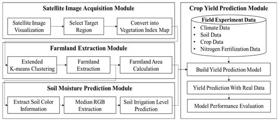
Figure 1.
The proposed framework for developing a crop yield prediction model using satellite imagery.
2.1. Farmland Extraction Module Using Satellite Images
Satellite imagery for the farmland extraction module is collected from Sentinel-2 images provided by ArcGIS online version [20]. Sentinel-2, operated by the European Space Agency (ESA), is a high-resolution Earth observation satellite that provides multispectral images with spatial resolutions ranging from 10 m to 60 m [21]. With 13 spectral bands covering not only the visible spectrum but also the near-infrared (NIR) and shortwave infrared (SWIR) spectrums, Sentinel-2 imagery is highly suitable for analyzing crop vegetation conditions [22]. In this study, the Red, NIR, and SWIR bands are selected because they provide effective information for farmland extraction. Based on these bands, vegetation indices are computed and subsequently transformed into vegetation maps. Table 1 describes the central wavelengths and spatial resolution of the selected three bands. The red band has the shortest central wavelength and belongs to the visible region, whereas the NIR and SWIR band lies within the infrared region. The red and NIR bands, both with a spatial resolution of 10 m, provide precise spatial detail, which is advantageous for farmland extraction. However, the SWIR band has a lower spatial resolution of 20 m, which requires resolution resampling across bands. In this study, the SWIR band was resampled to 10 m resolution using bilinear interpolation, reflecting the continuous variation in vegetation indices [23]. In addition, the solar zenith of the satellite imagery ranged from 30° to 45°, and the solar azimuth ranged from 40° to 90°. To ensure data quality, satellite images with more than 10% overall cloud coverage were excluded before farmland extraction.

Table 1.
Band information of Sentinel-2 satellite used in this study.
The main vegetation indices used for farmland extraction in this study are the Normalized Difference Vegetation Index (NDVI) and the Normalized Difference Moisture Index (NDMI). NDVI is a vegetation index that quantifies vegetation density and vigor on a scale from −1 to 1, and Equation (1) defines its calculation using the NIR and red bands [24]. Figure 2 shows the NDVI map of Haenam-gun, Jeollanam-do, South Korea (34.655° N, 126.429° E), generated from satellite imagery. Higher NDVI values indicate dense and healthy vegetation, which appear closer to green, whereas lower values correspond to sparse or no vegetation, appearing closer to brown. Due to these characteristics, NDVI image is widely applied in estimating plant stress and distinguishing farmland [25].
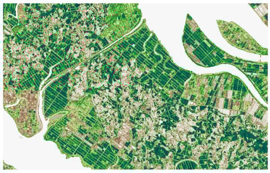
Figure 2.
NDVI map generated from satellite imagery.
NDMI is a vegetation index that represents the degree of crop water stress on a scale from −1 to 1, and Equation (2) presents its calculation using the NIR and SWIR bands [26]. Figure 3 illustrates the NDMI map of Haenam-gun, Jeollanam-do, South Korea (34.655° N, 126.429° E) generated from satellite imagery. Higher NDMI values indicate healthy vegetation with low water stress, which appear in blue tones, whereas lower values correspond to weakened vegetation with high water stress, appearing in white tones [27]. Thus, NDMI can serve as a valuable indicator for assessing crop water status and vegetation health, making it useful for farmland extraction.
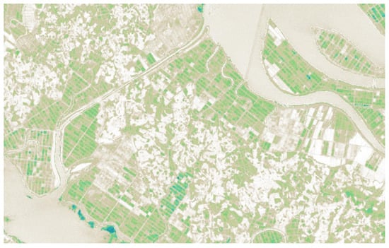
Figure 3.
NDMI map generated from satellite imagery.
The farmland area is calculated using NDVI and NDMI maps generated from satellite imagery. They exhibit distinct color contrasts between farmland and adjacent land types, and these differences are utilized to extract farmland. For this purpose, the unsupervised learning technique K-Means Clustering is applied. Each pixel of the maps is converted into an RGB vector with values ranging from 0 to 255. K-Means Clustering then assigns each data point to the nearest cluster center and determines the configuration that minimizes the within-cluster sum of squared distances [28]. Equation (3) represents the formula for classifying satellite images into two clusters.
where denotes the centroid of cluster k, is the set of clusters, and is the RGB vector of the i-th pixel.
Figure 4 shows the process of extracting farmland using NDVI and NDMI maps. NDVI map highlights vegetated areas in green tones, whereas NDMI map highlights areas with sufficient moisture in blue tones. K-Means Clustering is applied to each image separately, and only the intersection of NDVI and NDMI-based results are selected as the final farmland areas. The extracted farmland is computed on a pixel basis and subsequently converted into actual area units (m2) for further analysis.
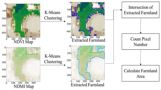
Figure 4.
Farmland extraction process using vegetation index maps from satellite imagery.
The performance of the farmland extraction module is evaluated by comparing the extracted farmland area with the actual farmland area. Four evaluation metrics which are the coefficient of determination (R2), mean absolute error (MAE), mean absolute percentage error (MAPE), and root mean squared error (RMSE) are used. MAE, RMSE, and MAPE are error-based metrics, where lower values indicate better performance. R2, on the other hand, measures the explanatory power of the model on a scale from 0 to 1, with values closer to 1 indicating stronger explanatory power. Equations (4)–(7) present the formulas used to calculate each metric.
where n denotes the total data point, yi is the actual farmland area, is the extracted farmland are, and represents the mean of the actual farmland area.
In addition to quantitively evaluate the accuracy of the extracted farmland area, the classification performance between farmland and non-farmland was further verified. Four evaluation metrics which are accuracy, precision, recall, and f1-score were employed and Equations (8)–(11) presents the formulas used to calculate each metrics.
where true positive (TP) refers to the cases where the positive label is correctly predicted as positive, and true negative (TN) refers to the cases where the negative label is correctly predicted as negative. In contrast, false positive (FP) and false negative (FN) refer to cases where the actual label is positive and negative, respectively, but it is predicted incorrectly. In this study, the positive label was defined as a farmland pixel, and the negative label as a non-farmland pixel. Accordingly, accuracy represents the proportion of correctly predicted pixels among all pixels, precision denotes the proportion of predicted farmland pixels that were actually farmland. Recall indicates the proportion of actual farmland pixels that were correctly predicted as farmland, and F1-score is the harmonic mean of precision and recall.
2.2. Soil Moisture Prediction Module
After extracting farmland using NDVI and NDMI maps (see Section 2.1), this study extracts soil color information (RGB), a physical characteristic, by mapping these areas onto satellite imagery from the pre-planting season. Soil color is directly influenced by soil moisture content, which can be used as an indicator of changes in irrigation levels. Irrigation level refers to the degree of moisture supply required for crop growth. For example, a 50% irrigation level supplies half of the crop’s moisture requirement, while a 100% irrigation level supplies the entire amount [29]. Soil moisture content increases gradually with irrigation level, being lowest at 0%, and highest at 100%. Generally, soil appears darker when moisture content is higher, and lighter when moisture content is lower. Therefore, RGB color information, which represents soil color, shows a strong correlation with soil moisture [30]. Soil color differences are particularly pronounced before crop growth begins, making it effective for distinguishing irrigation levels. Therefore, this study utilizes soil RGB values to estimate irrigation levels. Figure 5 shows the process of estimating irrigation levels based on soil color from detected farmland, and divides the irrigation levels of farmland into 100%, 50%, and 0%.
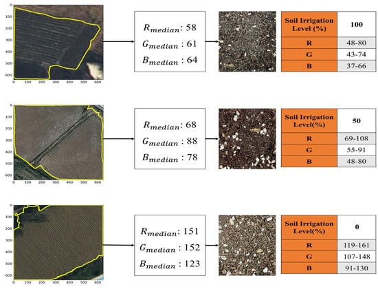
Figure 5.
Process of estimating irrigation level using soil color information of extracted farmland.
To extract RGB values from detected farmland, this study calculates the median RGB value based on the pixel distribution across the entire image, as shown in Equation (12), and uses it as a representative value. This is because unsupervised learning-based satellite image detection processes can contain outliers within agricultural fields, and while the mean is sensitive to these outliers, the median can effectively mitigate their impact.
where represents the Red value of a specific pixel n in the extracted farmland; represents the Green value of a specific pixel n in the extracted farmland; and represents the Blue value of a specific pixel n in the extracted farmland.
To establish a reference range for RGB values according to soil irrigation levels, this study directly controlled soil moisture and examined RGB changes by irrigation level. To this end, soil images were captured at 0%, 50%, and 100% irrigation levels, and quartiles were calculated for all pixels. The median (Q2) and third quartile (Q3) values were used to establish the RGB value range, while the first quartile (Q1) and fourth quartile (Q4) values were excluded due to their high likelihood of containing outliers.
2.3. Crop Yield Prediction Module
This study utilizes the Ensemble learning technique to predict crop yields. Ensemble learning combines multiple prediction models to achieve improved performance compared to a single model [19]. The Ensemble learning has the advantage of complementing the weaknesses of individual models to enhance generalization performance [31], and it includes bagging, boosting, and stacking approaches. This study adopts the stacking ensemble approach. Stacking ensemble learning involves inputting predictions derived from multiple base learners into a meta-learner to perform the final prediction [32]. The base learners and meta-learners are connected in a serial structure, and the base learners, each comprising a different machine learning algorithm, train and predict on the same input dataset. The prediction results from the base learner are then used as input to the meta-learner, ultimately improving the model’s prediction performance. Meanwhile, stacking ensembles pose a risk of overfitting when combining multiple base learners. Therefore, this study applied K-fold cross-validation to mitigate overfitting and ensure that all data is evenly utilized during the training process [33]. Figure 6 illustrates the process of applying K-fold cross-validation in a stacking ensemble.
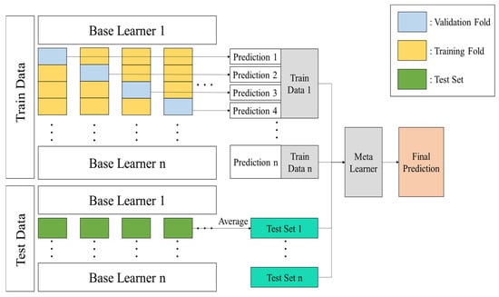
Figure 6.
Structure of stacking ensemble using k-fold cross-validation.
In Figure 6, the entire dataset is divided into training and test data. The training data is then divided into K folds, of which (K − 1) folds are used for model training, and the remaining one is used as a validation fold to evaluate model performance. This process is repeated K times, and since every sample in the training data is included in the validation fold once, predictions for the entire training data can be obtained. Each base learner generates predictions for the training data through this process, and these predictions are combined (stacked) and used as training data for the meta-learner. For the test data, the base learners are trained in each fold individually make predictions, and the average of the resulting predictions is an input as the test data for the meta-learner. This process ensures that all data are utilized in a balanced manner during the training and validation processes, mitigates the over-fitting problem to specific data, and improves model’s generalization performance. Finally, the developed model is applied to actual crop yield data to evaluate its final performance.
3. Results
3.1. Farmland Extraction Performance
To verify the performance of a satellite image-based farmland detection model, this study conducted an experiment in Haenam County, South Jeolla Province. This region is a major onion producing area in South Korea. Considering crop’s growth period, satellite image data was collected in September 2024, when vegetation begins to develop after sowing. Table 2 illustrates the soil properties of the selected area, categorized by soil depth into physical and chemical properties. The physical properties include the particle distribution (i.e., clay, silt, and sand), bulk density, and soil type. In both the surface layer (0–18 cm) and the subsurface layer (18–34 cm), silt accounts for the highest proportion, showing a similar distribution pattern between the two layers. The bulk density is higher in the subsurface layer (1.42 Mg/m3) compared to the surface layer (1.19 Mg/m3), and the soil types are classified as clay loam and silt loam, respectively. In addition, the field capacity, which represents the amount of soil moisture available for crop growth, was 35.7% in the surface layer and 36.0% in the subsurface layer. The chemical properties include organic carbon, cation exchange capacity, and potential of hydrogen (pH). The pH values of the surface and subsurface layers are 5.4 and 5.7, respectively, indicating slightly acidic soil in both layers. In addition, the organic carbon content in the surface layer (12.7 g/kg) is twice higher compared to the subsurface layer (5.6 g/kg).
Table 2.
Soil properties of Haenam County, South Jeolla Province [34].
To compare with the extracted farmland, the actual farmland was labeled by areas interpreted as farmland through satellite images. Table 3 describes a comparison of farmland detection performance by satellite image type. Using RGB images alone resulted in the lowest R2 of 0.683, limiting the ability to distinguish between farmland and non-farmland. In contrast, NDVI and NDMI vegetation maps significantly improved extraction accuracy by better reflecting farmland vegetation characteristics. Specifically, using NDVI images resulted in R2 of 0.908, approximately 32.9% higher accuracy than RGB images. Utilizing the overlapping area between NDVI and NDMI resulted in the highest detection performance, with R2 of 0.981. This represents an approximately 43.6% improvement over RGB images alone and an 8% improvement over NDVI images alone. Additionally, MAPE, MAE, and RMSE were the lowest at 0.126, 255.673, and 364.663, respectively, showing that the error between the predicted value and the actual value was minimized. This is because RGB images misclassified areas such as adjacent bare land or roads that have similar colors spectrum to farmland, leading to boundary errors. However, the vegetation index (i.e., NDVI, NDMI) reflected the spectral characteristics of farmland and achieved higher accuracy in intersection areas by complementing each other through the use of two different vegetation indices.
Table 3.
Performance of farmland detection using different types of satellite imagery.
Table 4 describes the result of verifying localization error and evaluating classification performance by comparing extracted farmland with actual farmland. Consistent with the results in Table 3, the highest accuracy was achieved when utilizing the intersection of NDVI and NDMI vegetation index maps, which is approximately 17% higher than when using RGB image (0.822). Meanwhile, recall, which represents the proportion of actual farmland among detected farmland, was highest at 1.000 for RGB and NDMI vegetation index map. However, precision was lowest for RGB image, which is because surrounding non-farmland pixels were detected as farmland. F1-score was also highest for the intersection of NDVI and NDMI images (0.953), which is approximately higher than RGB image (0.801).
Table 4.
Localization error of farmland detection using different types of satellite imagery.
3.2. Soil Moisture Prediction Performance
To verify how soil color varies with irrigation levels at the subject area (see Section 3.1), the RGB value distribution of all pixels was analyzed under different irrigation levels. Figure 7 shows the RGB distributions extracted at 0%, 50%, and 100% irrigation levels, which serves as the basis for establishing the reference ranges described in Section 2.2. For the 0% irrigation level, the RGB channel values exhibited a wide distribution (see Figure 7a). Although a large number of pixels with low values were observed in the blue channel, the overall distribution across all three channels appeared relatively normal. However, for the 50% and 100% irrigation levels (see Figure 7b,c), the RGB pixel distribution showed a right skewed pattern. This is because higher irrigation levels increase soil moisture content, which darkens the soil color and causes pixel values to concentrate in the lower range. In particular, at the 100% irrigation level, this became more evident, with nearly 50% of the pixels concentrated in the 0–50 value range. Although the distribution of RGB values varied with each irrigation level, overlapping ranges were observed. For example, the average overlap ratio of RGB values between 0% and 100% irrigation level was approximately 66%. In contrast, the average overlap ratio between 50% and 100% irrigation levels was higher at about 82%. These results indicate that soil moisture content directly influences soil color, and that higher irrigation levels lead to darker soil with lower pixel values.
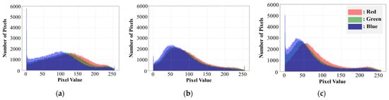
Figure 7.
Distribution of RGB values across all pixels under different irrigation levels: (a) 0% irrigation level, (b) 50% irrigation level, (c) 100% irrigation level.
Based on the distributions identified under each irrigation level, the median (Q2) and third quartile (Q3) values of the RGB channels were extracted to establish the reference ranges. Table 5 describes the ranges of RGB channels under different irrigation levels. As the irrigation level increased, the minimum and maximum RGB values generally decreased. This reflects the characteristic that increasing irrigation levels increases soil moisture, and that soils generally appear darker as moisture content increases. In particular, RGB values tended to decrease steeply when the irrigation level increased from 0% to 50%, and the maximum Green value decreased the most during this process. If the RGB values of the extracted farmland fell within the reference range, it was classified into the corresponding irrigation level, and the classified RGB values were utilized as feature variables reflecting soil moisture.
Table 5.
RGB value range under different soil irrigation levels.
3.3. Onion Yield Prediction Performance
To verify the performance of the stacking ensemble-based onion yield prediction model proposed in this study, yield data were collected according to changes in soil environmental factors [35,36,37,38]. The data corresponding to 2009, 2013–2014, and 2021–2023 from four field studies conducted at different locations were collected for the proposed staggered ensemble learning. The soil irrigation levels of the collected data ranged from 50 to 100% and the nitrogen fertilizer rates ranged from 0 to 184 kg/ha. As with other machine learning techniques, to create a model with high predictive accuracy by learning clear relationships between multiple independent variables (soil moisture and climate factors) and the dependent variable (onion yield), it is necessary to utilize multiple datasets to build a more generalizable model [39]. Table 6 describes the meteorological data during the onion growing season in each study. The average temperature was lowest in Study B and highest in Study A. The average daily precipitation ranged from 1.48 to 3.23 mm/day, and the average relative humidity and solar irradiance were observed to be 59.57% and 21.64 MJ/m2/day, respectively. Although all four datasets were collected in Ethiopia, there were differences in meteorological conditions. These differences in weather and soil environmental conditions were major factors influencing onion yield fluctuations, and in this study, two factors were considered simultaneously to reflect this.
Table 6.
Weather information for collected datasets.
The collected data was used as input for an onion yield prediction model. A stacking ensemble technique was applied for prediction, with 80% of the total dataset assigned as training data and the remaining 20% as test data. In this study, five different regression prediction algorithms (i.e., support vector regressor (SVR), least absolute shrinkage and selection operator (Lasso) regression, linear regression (LR), decision tree regressor (DTR), and random forest regressor (RFR)) were set as metamodels to examine changes in prediction performance. All models were optimized through hyperparameter tuning and tested.
The models were compared under two conditions: the Irrigation Level Model, which directly utilized soil irrigation levels as input variables; and the Satellite RGB Model, which extracted RGB values for each soil irrigation level from satellite images using the method proposed in this study and replaced these values with input variables. Table 7 describes the performance comparison results according to metamodel changes under both conditions. In the Irrigation Level Model, when DTR was applied as a metamodel, the R2 was 0.7656, showing the lowest performance, and when Lasso was applied as a metamodel, the R2 was 0.9420, showing the highest performance. Compared to Lasso, the R2 of DTR was approximately 17.6% lower, and the MAE and RMSE were also 1.7036 and 1.2532 higher, respectively. On the other hand, in the Satellite RGB Model, when SVR was applied as a metamodel, the R2 was 0.9839, showing the highest performance, and when RFR was applied as a metamodel, the R2 was 0.9368, showing the lowest performance. Overall, the average R2 (0.9688) for all metamodels in the Satellite RGB Model was approximately 8.3% higher than that of the Irrigation Level Model (0.8944). In particular, when SVR was applied to the Satellite RGB Model, the result was approximately 4.4% improved compared to the best performance of the Irrigation Level Model. These results highlight the importance of selecting an appropriate metamodel in a stacking ensemble, and, in particular, more accurate predictions can be achieved when RGB values extracted from satellite images are used as input variables rather than directly inputting soil irrigation levels.
Table 7.
Comparison of meta learner performance across Irrigation Level and Satellite RGB Model.
Figure 8 shows the results of comparing the R2 of each base learner in the Irrigation Level Model and Satellite RGB Model. The performance index of each learner was calculated as the average of the values produced through 5-fold cross validation. In the Irrigation Level Model, the base learners with the highest performance were LR and Lasso, both recording R2 of 0.9167. This is approximately 45.4% higher than DTR (0.6306), which showed the lowest R2. In contrast, in the Satellite RGB Model, SVR showed the highest performance with R2 of 0.8063, which is approximately 41.9% higher than DTR (0.5683), which showed the lowest R2. Overall, the base learner of the Irrigation Level Model outperforms the base learner of the Satellite RGB Model. In particular, SVR, which showed the highest R2 in the Satellite RGB Model, was approximately 12.0% lower than LR and Lasso, which showed the highest accuracy in the Irrigation Level Model. However, as can be seen in the results in Table 7, the Satellite RGB Model showed higher performance when the metamodel was applied, even though the base learner’s performance was lower than that of the Irrigation Level Model. This shows that the stacking ensemble technique effectively complements the limitations of individual base learners, and is particularly suitable for the Satellite RGB Model.
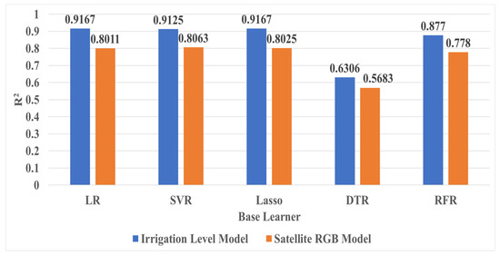
Figure 8.
Comparison of base learner performance across Irrigation Level and Satellite RGB Model.
Figure 9 compares the actual and predicted yields when SVR was used as a meta-learning tool in the Satellite RGB Model, which showed the highest prediction accuracy, as shown in Table 7. Note that there are eight test datasets (or test datasets from eight folds) used for the model evaluation in Figure 9 (see Section 2.3). Overall, the actual and predicted yields showed similar trends. Despite the different distributions of actual yields across cases, the model reflected this variability well and reliably predicted yields at various levels. In particular, Case 4 predicted yields most accurately, with a prediction error of approximately 0.02 ton/ha. Conversely, Case 1 showed the largest discrepancy between the predicted and actual yields.
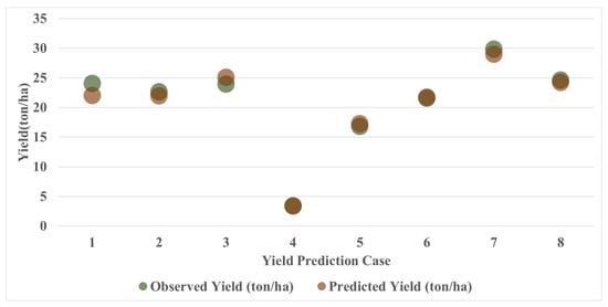
Figure 9.
Comparison of predicted and actual yields by the Satellite RGB Model (SVR as Meta-Learner).
4. Discussion
In Section 3, this study conducted a performance evaluation of the three modules (farmland extraction module, soil moisture prediction module, and crop yield prediction module) proposed in Section 2. Farm detection using satellite imagery to remotely detect and easily monitor farms was conducted. To improve farm detection performance and facilitate easy monitoring, satellite imagery was used to detect farms remotely. Two vegetation indices, the Normalized Difference Vegetation Index (NDVI) and the Normalized Difference Water Index (NDMI), were utilized. Farms were detected using the K-means clustering technique. For the selected Haenam onion farm area in South Korea, the system demonstrated a 43.63% improvement in farm detection performance (R2 value: 0.981) compared to the existing RGB imagery (R2 value: 0.683). This demonstrates that the utilization of satellite imagery, which is increasingly being used for precision agriculture, can improve existing farm detection performance.
In addition, this study analyzed RGB values that change with soil moisture content by mapping farmland to standard satellite imagery and analyzing the physical characteristics of soil (RGB). Furthermore, it provided a table of RGB changes based on soil moisture. Soil color is known to be directly affected by soil moisture content. Section 3.2 demonstrated that even in soils with the same RGB distribution, the distribution can actually change depending on moisture content [29]. However, because this study only considered RGB changes in soil for a specific region, separate experimental data collection is necessary as the research subject changes. In addition, satellite images are affected by the seasonal solar altitude which results in illumination and shadow [40]. Since these factors can interfere with the consistent color characteristics of soil, image balancing should be applied to ensure generalization. Despite these limitations, once the dataset is constructed and the proposed RGB-based soil moisture prediction model is properly calibrated, it can remotely predict soil moisture conditions in farms. This has the advantage of reducing crop production costs and improving yields through optimal irrigation.
Finally, an onion yield prediction model was developed using a staggered ensemble learning method based on predicted soil moisture content and climate data. The performance of the irrigation level model, which directly utilizes soil irrigation levels as input variables, was compared with the satellite RGB model, which extracts RGB values for each soil irrigation level from satellite images using the proposed method and replaces these values with input variables. Ensemble learning demonstrated differences in performance across models. For the irrigation level model, applying Lasso as the metamodel yielded the highest performance, with an R2 of 0.9420. For the Satellite RGB model, applying SVR as the metamodel yielded the highest performance, with an R2 of 0.9839, demonstrating the superiority of the proposed methodology. In particular, since performance differences depend on the selection of the appropriate metamodel in the stacking ensemble, we found that future modeling requires appropriately selecting a metamodel pool. Furthermore, we found that using RGB values extracted from satellite images as input variables instead of directly inputting soil irrigation levels yielded more accurate predictions.
5. Conclusions
This study proposes a satellite image-based soil moisture and onion yield prediction technique, enabling remote, preventative soil moisture management using readily available satellite images. Specifically, this technique enables individual farms to implement efficient irrigation policies to effectively prevent soil drying due to soil pressure and rising temperatures. The proposed methodology utilizes K-means clustering to accurately detect remote farmland using two vegetation indices (Normalized Difference Vegetation Index (NDVI) and Normalized Difference Moisture Index (NDMI)) from satellite data. This enables remote farm management by commercial farmers operating large-scale farms or companies managing overseas farmland. The extracted farmland is mapped to standard satellite images to extract color information (RGB), a physical characteristic of soil. This allows the RGB-based soil moisture content reference table proposed in this study to predict observed soil moisture content. Finally, crop yield prediction was performed based on soil moisture and climate data using the staggered ensemble learning technique. The highest R2 value for soil moisture content prediction was 0.9420 in the Lasso model, and the highest R2 value for yield prediction was 0.9839 in the SVR model. The results of this study demonstrate that the proposed methodology can enable precise agricultural management using satellite imagery despite utilizing relatively simple machine learning techniques. In particular, in Korea, the agricultural population is gradually decreasing, making it difficult to manage large-scale farms. Therefore, monitoring soil irrigation levels and crop yield through remote sensing can serve as an effective solution.
To apply the proposed methodology to a wider range of regions in the future, a separate RGB reference table needs to be created to account for regional differences in soil composition and color. Further research is needed in this area. Furthermore, continuous performance improvement is needed by considering a wider range of algorithms in ensemble learning.
Author Contributions
Conceptualization, S.K. (Sojung Kim), S.K. (Sumin Kim); methodology, S.K. (Sojung Kim), S.K. (Sumin Kim), J.S.; software, J.S.; validation, S.K. (Sojung Kim), S.K. (Sumin Kim), J.S.; resources, S.K. (Sumin Kim); writing—original draft preparation, S.K. (Sojung Kim), J.S., S.K. (Sumin Kim); writing—review and editing, S.K. (Sojung Kim), J.S., S.K. (Sumin Kim); visualization, J.S.; project administration, S.K. (Sojung Kim); funding acquisition, S.K. (Sojung Kim), S.K. (Sumin Kim). All authors have read and agreed to the published version of the manuscript.
Funding
This work was carried out with the support of “Cooperative Research Program for Agriculture Science and Technology Development (Project No. RS-2024-00394437)” funded by Rural Development Administration, Republic of Korea.
Data Availability Statement
The original contributions presented in the study are included in the article, further inquiries can be directed to the corresponding author.
Acknowledgments
The authors gratefully acknowledge the support of the Rural Development Administration, Republic of Korea. The views expressed in this paper are solely those of the authors and do not represent the opinions of the funding agency.
Conflicts of Interest
The authors declare no conflicts of interest.
References
- Food and Agriculture Organization of the United Nations. Small Family Farmers Produce a Third of the World’s Food. Available online: https://www.fao.org/newsroom/detail/Small-family-farmers-produce-a-third-of-the-world-s-food/en (accessed on 27 September 2025).
- Food and Agriculture Organization (FAO). Agricultural Trade, Trade Policies and the Global Food System. Available online: https://www.fao.org/4/y4252e/y4252e11.htm (accessed on 21 October 2025).
- Grainrus. Which Countries in the World Have the Most Developed Agriculture? Available online: https://grainrus.com/en/news/articles/v-kakikh-stranakh-mira-naibolee-razvito-selskoe-khozyaystvo/#:~:text=profitable%20agricultural%20production?-,Top%20Five%20Agricultural%20Countries,the%20top%20five%20agricultural%20countries (accessed on 27 September 2025).
- Bloom Ranch. Advantages and Disadvantages of Commercial Farming. Available online: https://bloomranchofacton.com/pages/advantages-and-disadvantages-of-commercial-farming-including-definition-examples-images-types (accessed on 27 September 2025).
- Kim, Y.; On, Y.; So, J.; Kim, S.; Kim, S. A Decision support software application for the design of agrophotovoltaic systems in Republic of Korea. Sustainability 2023, 15, 8830. [Google Scholar] [CrossRef]
- Li, X.; Wang, R.; Du, Y.; Han, H.; Guo, S.; Song, X.; Ju, X. Significant increases in nitrous oxide emissions under simulated extreme rainfall events and straw amendments from agricultural soil. Soil Tillage Res. 2025, 246, 106361. [Google Scholar] [CrossRef]
- Gnisia, G.; Weik, J.; Ruser, R.; Essich, L.; Lewandowski, I.; Stein, A. Machine learning-based prediction of nitrous oxide emissions from arable farming: Exploring management practices as predictor variables. Ecol. Indic. 2025, 172, 113233. [Google Scholar] [CrossRef]
- Akkem, Y.; Biswas, S.K.; Varanasi, A. Smart farming using artificial intelligence: A review. Eng. Appl. Artif. Intell. 2023, 120, 105899. [Google Scholar] [CrossRef]
- Centorame, L.; La Porta, N.; Papandrea, M.; Mancini, A.; Foppa Pedretti, E. Evaluation of Feature Selection and Regression Models to Predict Biomass of Sweet Basil by Using Drone and Satellite Imagery. Appl. Sci. 2025, 15, 6227. [Google Scholar] [CrossRef]
- Al-Gaadi, K.A.; Madugundu, R.; Tola, E.; El-Hendawy, S.; Marey, S. Satellite-based determination of the water footprint of carrots and onions grown in the arid climate of Saudi Arabia. Remote Sens. 2022, 14, 5962. [Google Scholar] [CrossRef]
- Dastagiri, M.; Naga Sindhuja, P.V. Satellite farming in global agriculture: New tech revolution for food security and planet safety for future generation. Sci. Agric. 2020, 4, 2–10. [Google Scholar] [CrossRef]
- Nguyen, T.T.; Hoang, T.D.; Pham, M.T.; Vu, T.T.; Nguyen, T.H.; Huynh, Q.-T.; Jo, J. Monitoring agriculture areas with satellite images and deep learning. Appl. Soft Comput. 2020, 95, 106565. [Google Scholar] [CrossRef]
- Segarra, J.; Buchaillot, M.L.; Araus, J.L.; Kefauver, S.C. Remote sensing for precision agriculture: Sentinel-2 improved features and applications. Agronomy 2020, 10, 641. [Google Scholar] [CrossRef]
- The Business Research Company. Satellite Data Service for Agriculture Global Market Report. Available online: https://www.thebusinessresearchcompany.com/report/satellite-data-service-for-agriculture-global-market-report (accessed on 27 September 2025).
- Yoo, J.; Ahn, J.; Han, K.; Kang, H.; Cho, H.; Jeong, Y. Utilization of satellite technologies for agriculture. J. Environ. Sci. Int. 2024, 33, 547–552. [Google Scholar] [CrossRef]
- Omia, E.; Bae, H.; Park, E.; Kim, M.S.; Baek, I.; Kabenge, I.; Cho, B.-K. Remote sensing in field crop monitoring: A comprehensive review of sensor systems, data analyses and recent advances. Remote Sens. 2023, 15, 354. [Google Scholar] [CrossRef]
- Zhang, H.; Liu, Y.; Zhang, C.; Li, N. Machine learning methods for weather forecasting: A survey. Atmosphere 2025, 16, 82. [Google Scholar] [CrossRef]
- Shiff, S.; Lensky, I.M.; Bonfil, D.J. Using satellite data to optimize wheat yield and quality under climate change. Remote Sens. 2021, 13, 2049. [Google Scholar] [CrossRef]
- Kim, Y.; Kim, S.; Kim, S. Onion (Allium cepa) Profit Maximization via Ensemble Learning-Based Framework for Efficient Nitrogen Fertilizer Use. Agronomy 2024, 14, 2130. [Google Scholar] [CrossRef]
- Environmental Systems Research Institute (ESRI). Sentinel-2 Explorer. Available online: https://livingatlas.arcgis.com/sentinel2explorer/#mapCenter=122.87724%2C-23.46876%2C11.000&mode=dynamic&mainScene=%7CAgriculture+for+Visualization%7C (accessed on 1 September 2025).
- Copernicus Data Space Ecosystem (CDSE). Sentinel-2. Available online: https://dataspace.copernicus.eu/data-collections/copernicus-sentinel-data/sentinel-2 (accessed on 1 September 2025).
- Xie, Q.; Dash, J.; Huete, A.; Jiang, A.; Yin, G.; Ding, Y.; Peng, D.; Hall, C.C.; Brown, L.; Shi, Y. Retrieval of crop biophysical parameters from Sentinel-2 remote sensing imagery. Int. J. Appl. Earth Obs. Geoinf. 2019, 80, 187–195. [Google Scholar] [CrossRef]
- Environmental Systems Research Institute (ESRI). Resample Function. Available online: https://pro.arcgis.com/en/pro-app/3.3/help/analysis/raster-functions/resample-function.htm (accessed on 13 October 2025).
- Amani, S.; Shafizadeh-Moghadam, H. A review of machine learning models and influential factors for estimating evapotranspiration using remote sensing and ground-based data. Agric. Water Manag. 2023, 284, 108324. [Google Scholar] [CrossRef]
- Huang, S.; Tang, L.; Hupy, J.P.; Wang, Y.; Shao, G. A commentary review on the use of normalized difference vegetation index (NDVI) in the era of popular remote sensing. J. For. Res. 2021, 32, 1–6. [Google Scholar] [CrossRef]
- Taloor, A.K.; Manhas, D.S.; Kothyari, G.C. Retrieval of land surface temperature, normalized difference moisture index, normalized difference water index of the Ravi basin using Landsat data. Appl. Comput. Geosci. 2021, 9, 100051. [Google Scholar] [CrossRef]
- Lykhovyd, P.; Sharii, V. Normalised difference moisture index in water stress assessment of maize crops. Agrology 2024, 7, 21–26. [Google Scholar] [CrossRef] [PubMed]
- Burney, S.A.; Tariq, H. K-means cluster analysis for image segmentation. Int. J. Comput. Appl. 2014, 96, 1–8. [Google Scholar] [CrossRef]
- Workie, A.G.; Ketsela, Y.S. Assessing irrigation water management utilizing the CROPGRO model in implementing deficit irrigation for peanut cultivation in Arba Minch, Ethiopia. Water Sci. 2025, 39, 138–150. [Google Scholar] [CrossRef]
- Zheng, L.; Li, M.; Sun, J.; Tang, N.; Zhang, X. Estimation of soil moisture with aerial images and hyperspectral data. In Proceedings of the 2005 IEEE International Geoscience and Remote Sensing Symposium, Seoul, Republic of Korea, 29 July 2005; pp. 4516–4519. [Google Scholar]
- Martinez, W.G. Ensemble pruning via quadratic margin maximization. IEEE Access 2021, 9, 48931–48951. [Google Scholar] [CrossRef]
- Liu, L.; Zhao, G.; Liang, W.; Jian, Z. Hybrid stacking ensemble algorithm and simulated annealing optimization for stability evaluation of underground entry-type excavations. Undergr. Space 2024, 17, 25–44. [Google Scholar] [CrossRef]
- Lu, M.; Hou, Q.; Qin, S.; Zhou, L.; Hua, D.; Wang, X.; Cheng, L. A stacking ensemble model of various machine learning models for daily runoff forecasting. Water 2023, 15, 1265. [Google Scholar] [CrossRef]
- Soil Environment Information System. Soil Properties. Available online: https://soil.rda.go.kr/soilmap/chemistry.do (accessed on 28 September 2025).
- Fitsum, G.; Woldetsadik, K.; Alemayhu, Y. Effect of irrigation depth and nitrogen levels on growth and buld yield on onion (Allium cepa L) at algae, central rift valley of Ethiopia. Int. J. Life Sci. 2016, 5, 152–162. [Google Scholar]
- Ambomsa, A.; Husen, D.; Shelemew, Z.; Jalde, A. Effects of Different Irrigation Levels and Fertilizer Rates on Yield, Yield Components and Water Productivity of Onion at Adami Tulu Agricultural Research Center. Agric. For. Fish. 2023, 12, 57–63. [Google Scholar] [CrossRef]
- Kemal, Y.O. Effects of irrigation and nitrogen levels on bulb yield, nitrogen uptake and water use efficiency of shallot (Allium cepa var. ascalonicum Baker). Afr. J. Agric. Res. 2013, 8, 4637–4643. [Google Scholar] [CrossRef][Green Version]
- Lindi, S.; Nanesa, K.; Hone, M.; Eticha, B. Determination of Irrigation Scheduling and Optimal Nitrogen Fertilizer Rate for Onion in Tiyo District, Arsi Zone, South Eastern Ethiopia. Global Res. Environ. Sustainability 2024, 2, 15–27. [Google Scholar]
- Kim, S.; Seo, J.; Kim, S. Machine learning technologies in the supply chain management research of biodiesel: A review. Energies 2024, 17, 1316. [Google Scholar] [CrossRef]
- Liu, J.; Wang, X.; Chen, M.; Liu, S.; Shao, Z.; Zhou, X.; Liu, P. Illumination and contrast balancing for remote sensing images. Remote Sens. 2014, 6, 1102–1123. [Google Scholar] [CrossRef]


Disclaimer/Publisher’s Note: The statements, opinions and data contained in all publications are solely those of the individual author(s) and contributor(s) and not of MDPI and/or the editor(s). MDPI and/or the editor(s) disclaim responsibility for any injury to people or property resulting from any ideas, methods, instructions or products referred to in the content. |
© 2025 by the authors. Licensee MDPI, Basel, Switzerland. This article is an open access article distributed under the terms and conditions of the Creative Commons Attribution (CC BY) license (https://creativecommons.org/licenses/by/4.0/).