Monitoring the Maize Canopy Chlorophyll Content Using Discrete Wavelet Transform Combined with RGB Feature Fusion

Abstract

To evaluate the accuracy of Discrete Wavelet Transform (DWT) in monitoring the chlorophyll (CHL) content of maize canopies based on RGB images, a field experiment was conducted in 2023. Images of maize canopies during the jointing, tasseling, and grouting stages were captured using unmanned aerial vehicle (UAV) remote sensing to extract color, texture, and wavelet features and to construct a color and texture feature dataset and a fusion of wavelet, color, and texture feature datasets. Backpropagation neural network (BP), Stacked Ensemble Learning (SEL), and Gradient Boosting Decision Tree (GBDT) models were employed to develop CHL monitoring models for the maize canopy. The performance of these models was evaluated by comparing their predictions with measured CHL data. The results indicate that the dataset integrating wavelet features achieved higher monitoring accuracy compared to the color and texture feature dataset. Specifically, for the integrated dataset, the BP model achieved an R² value of 0.728, an RMSE of 3.911, and an NRMSE of 15.24%; the SEL model achieved an R² value of 0.792, an RMSE of 3.319, and an NRMSE of 15.34%; and the GBDT model achieved an R² value of 0.756, an RMSE of 3.730, and an NRMSE of 15.45%. Among these, the SEL model exhibited the highest monitoring accuracy. This study provides a fast and reliable method for monitoring maize growth in field conditions. Future research could incorporate cross-validation with hyperspectral and thermal infrared sensors to further enhance model reliability and expand its applicability.

1. Introduction

Maize (Zea mays L.), a primary cereal crop worldwide, is extensively grown in various regions. Its development and productivity are essential for maintaining global food security. The chlorophyll (CHL) content, a crucial physiological marker of crop health, plays a vital role in light absorption [1]. Therefore, accurately monitoring the CHL content is essential for optimizing crop yield. The Soil and Plant Analyzer Development (SPAD) value, which reflects the greenness of plants, is widely used as a reliable proxy for the CHL content [2]. Traditional methods for measuring CHL, such as spectroscopic absorption and chemical analysis, have been widely applied but face certain limitations [3,4]. The spectral absorption method relies on specific spectral bands, making its results susceptible to environmental factors such as weather conditions (e.g., cloud cover and lighting variability), soil variability (e.g., differences in moisture or organic content), and plant canopy structure. These factors can alter the reflectance and absorption characteristics of the measured light, thereby challenging the consistency and precision of the results. Chemical analysis, on the other hand, requires leaf sampling, which damages crops and is unsuitable for large-scale and rapid monitoring. These limitations highlight the need for innovative approaches such as unmanned aerial vehicle (UAV) remote sensing, which offers an efficient, scalable, and non-destructive solution to these challenges.

Remote sensing technology, particularly UAV-based remote sensing, offers innovative solutions for crop health monitoring [5,6]. While satellite remote sensing provides extensive coverage and long-term monitoring capabilities, it suffers from a low spatial resolution and limited timeliness under adverse weather conditions [7]. Ground-based remote sensing, such as handheld spectrometers, delivers accurate data but is inefficient and costly for large-scale applications. UAV remote sensing bridges these gaps by offering high spatial resolution and real-time monitoring, making it an essential tool for precise and large-scale agricultural monitoring [8,9,10]. For instance, Sun et al. [11] employed UAV multispectral imagery to monitor maize maturity levels in autumn. Similarly, Gautam et al. [12] used UAV multispectral data to show that high chlorophyll activity, which strongly reflects NIR wavelengths, leads to increased NDVI values in grapevine leaves in high- and medium-vigor zones. Njane et al. [13] evaluated plant height, volume, and NDVI using multispectral images captured by drones and found that lower flight altitudes enabled more accurate estimations of crop height and volume. Additionally, Li et al. [14] developed semi-automatic image analysis software to accurately estimate potato seedling emergence rates using UAV RGB imagery. Current research predominantly leverages UAV platforms equipped with RGB, multispectral, and hyperspectral sensors for crop phenotyping [15,16]. Among these, RGB sensors stand out due to their low cost, high spatial resolution, and spectral characteristics. The R, G, and B channels correspond to wavelengths associated with the absorption region of chlorophyll a and the reflection features of chlorophyll b, offering significant potential for agricultural monitoring. Despite being limited to the visible spectrum (400–700 nm), RGB sensors can still effectively extract crop growth information through appropriate data processing and analysis [17,18]. For example, Kou et al. [19] utilized UAV-acquired RGB imagery of cotton canopies at a 20 m altitude to extract features and construct a 2D CNN regression model, achieving accurate nitrogen content prediction in cotton canopies.

Wavelet transform, as an emerging image processing technique, decomposes RGB images into wavelet coefficients at various scales and directions, enabling the extraction of localized feature information from the image [20]. Compared to techniques like vegetation indices and spectral reflectance, Discrete Wavelet Transform (DWT) offers distinct advantages for chlorophyll content monitoring [21]. Vegetation indices are sensitive to atmospheric conditions and require calibration for different crop types, whereas DWT captures both spatial and frequency information, making it more robust. While spectral reflectance methods offer high accuracy, they require expensive equipment and complex preprocessing steps. In contrast, DWT uses widely available RGB images, offering a more efficient solution. The multi-resolution analysis capability of DWT allows for the extraction of both global features and local details, such as canopy texture and structural variations, thereby improving the accuracy of chlorophyll monitoring models [22,23]. DWT can be combined with features like color and texture to create a comprehensive dataset. This approach outperforms single-feature methods in model performance. These attributes make DWT highly significant and promising for advancing precision agriculture, particularly in real-time and scalable applications [24]. Although research on using DWT for maize canopy chlorophyll monitoring is still limited, the proven efficiency and adaptability of DWT underscore its potential. With the rapid development of image processing and machine learning, the importance of feature fusion has been demonstrated across many fields. Integrating different features, including texture, spectral bands, vegetation indices, and wavelet transforms, is a key method to enhance the accuracy of crop phenotyping [25].

This study utilizes UAV RGB sensors to capture maize canopy images from field crops, extracting color, texture, and wavelet features. It constructs datasets based on color and texture features as well as fused datasets combining wavelet, color, and texture features. The study then develops maize canopy chlorophyll content monitoring models using BP, SEL, and GBDT algorithms and identifies the optimal model. The specific objectives of this research are (1) to demonstrate the effectiveness of RGB feature fusion methods for chlorophyll content monitoring in maize canopies and (2) to evaluate the potential of DWT for chlorophyll content monitoring in maize canopies.

2. Materials and Methods

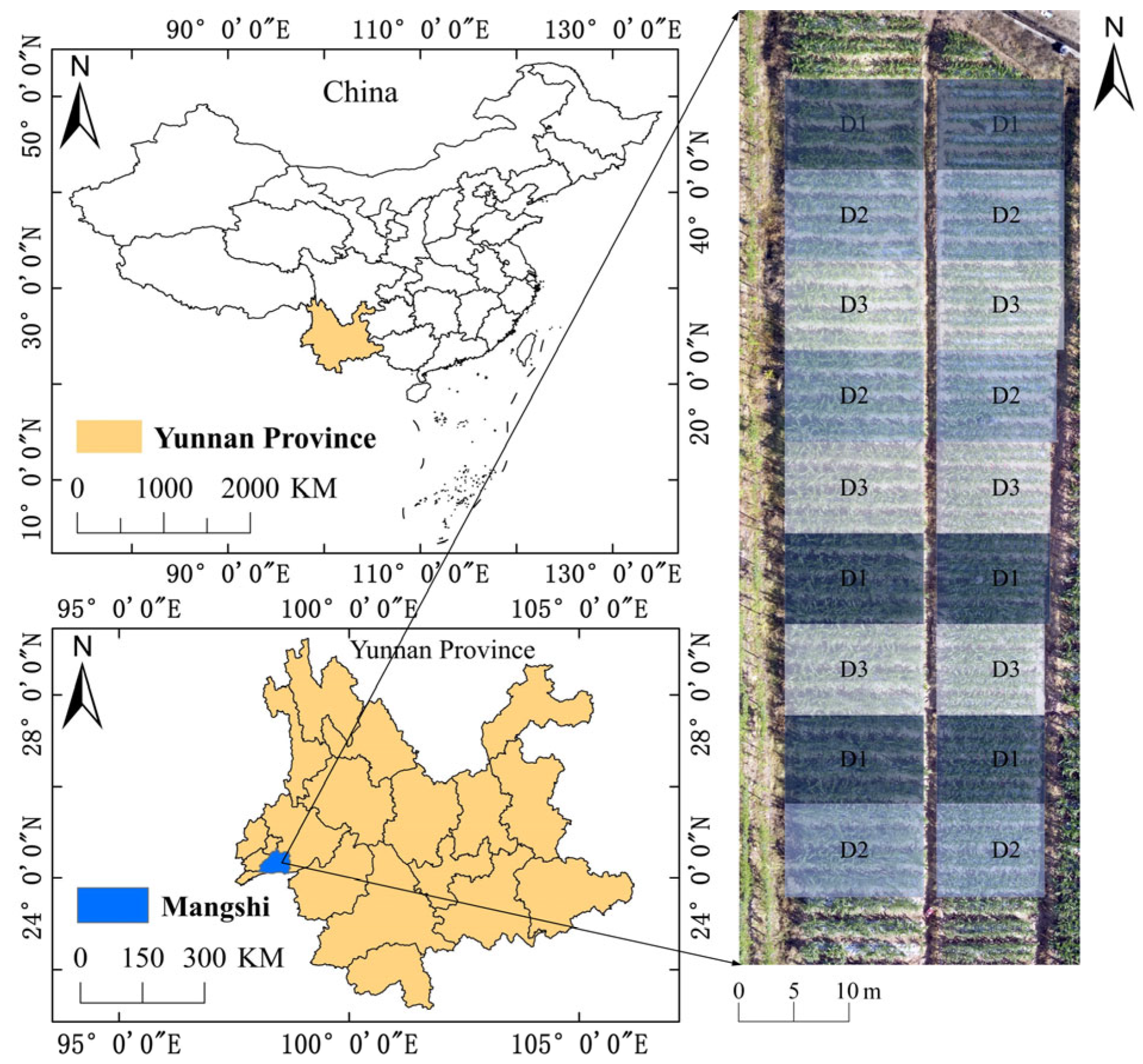
2.1. Study Area and Experimental Design

The field experiment was conducted in 2023 in Mangshi Daxingzhai (98°40′24″ E, 24°25′37″ N) and Mabozi Village (98°35′90″ E, 24°25′76″ N) in Dehong Prefecture, Yunnan Province, China (Figure 1). The region experiences a South Asian tropical monsoon climate, characterized by an average yearly temperature of 20.2 °C and an annual precipitation of 1659.3 mm. The soil in the experimental site is sandy loam with a pH of 7.27, containing 16.9 g/kg of organic matter, 72.1 mg/kg of available nitrogen, 15 mg/kg of available phosphorus, and 91.3 mg/kg of available potassium. The experiment utilized Beiyu 1521, a maize variety resistant to diseases. The sowing dates were 14 June 2023 and 14 July 2023, covering an area of around 1021 m². Three planting densities were implemented: 5.7 plants/m² (D1), 6.3 plants/m² (D2), and 6.9 plants/m² (D3). The row spacing for all densities was 70 cm, with plant spacings of 0.24 m, 0.227 m, and 0.207 m for D1, D2, and D3, respectively. Planting was repeated three times using randomized distribution. Pests and diseases can lead to localized leaf yellowing, affecting the canopy CHL content, interfering with feature extraction, and reducing model accuracy. Following emergence, pest control was carried out four times, with each application separated by a 10-day interval, alternating between lambda-cyhalothrin and chlorfenapyr. Other field management practices adhered to local agricultural standards.

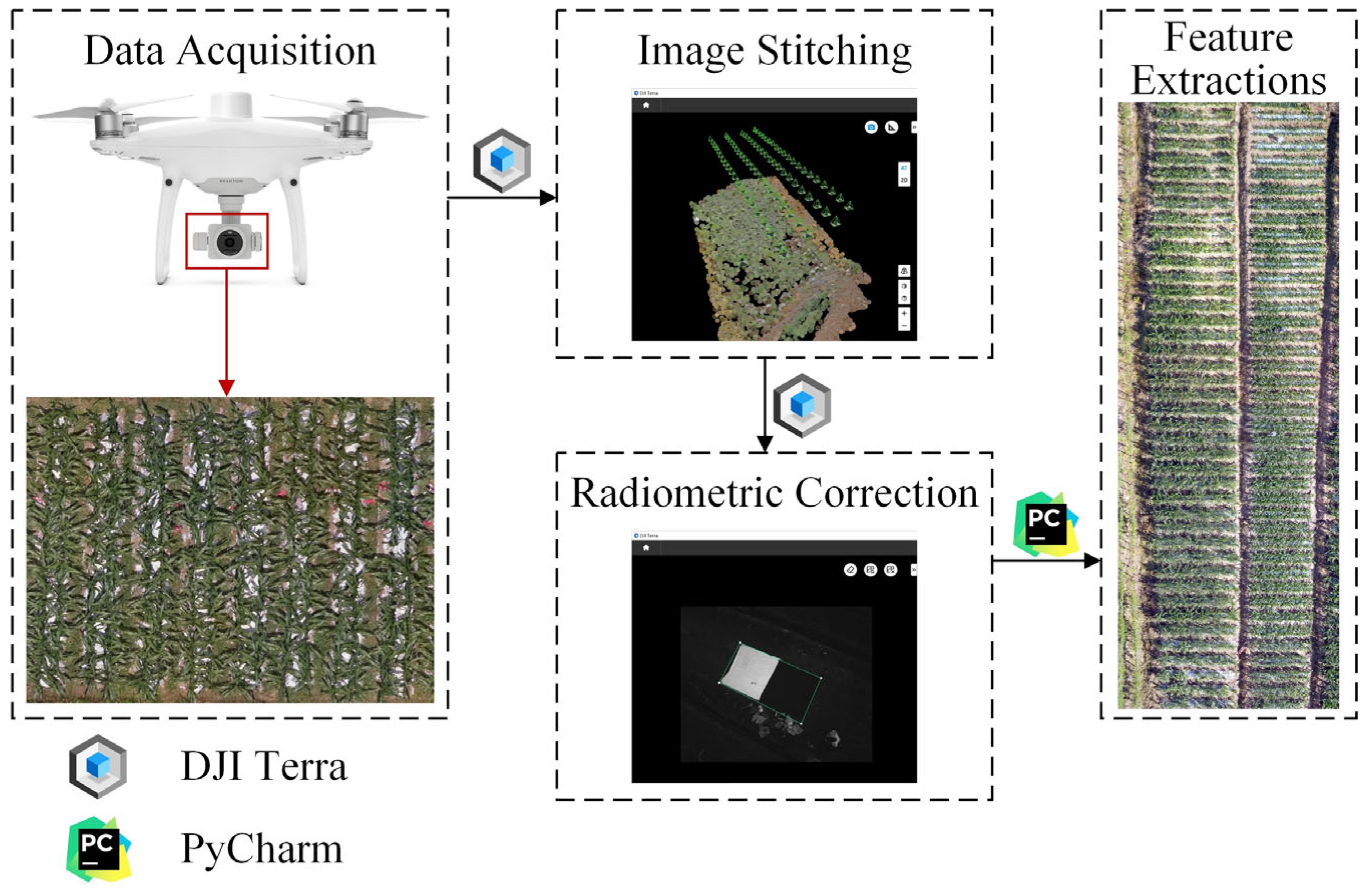
2.2. Acquisition and Processing of Aerial Images of Maize Canopy

Remote sensing data were collected using a DJI Phantom 4 RTK drone (SZ DJI Technology Co., Shenzhen, China) equipped with a 1-inch 20-megapixel CMOS sensor for capturing high-definition imagery. The final spatial resolution of the orthophoto was 766 × 2744. The camera of the DJI Phantom 4 RTK drone is pre-calibrated before shipment, eliminating the need for recalibration during routine use. However, if the UAV displays a “Vision System Abnormal” error, the camera can be recalibrated by connecting the UAV to a computer via a USB cable and using DJI Assistant 2 V1.2.5 software. The drone is also equipped with a light intensity sensor mounted on its top, which captures solar irradiance data and embeds them in the image files. During post-processing, these solar irradiance data can be used to compensate for lighting variations, thereby reducing the influence of environmental lighting on image quality.

Data collection was conducted during key maize growth stages, namely the jointing stage (17 July 2023), tasseling stage (3 August 2023), and grouting stage (17 August 2023), between 12:00 and 14:00. On 17 July, from 12:00 to 14:00, the temperature ranged from 28.08 °C to 29.39 °C with no precipitation. Horizontal surface radiation ranged from 922.99 W/m² to 943.99 W/m², and ground wind speed varied from 0.869 m/s to 1.145 m/s. On 3 August, from 12:00 to 14:00, the temperature ranged from 24.06 °C to 25.56 °C, with precipitation amounts in the range of 0.459 mm to 0.338 mm. Horizontal surface radiation ranged from 647.49 W/m² to 797.24 W/m², and ground wind speed varied from 1.449 m/s to 0.835 m/s. On 17 August, from 12:00 to 14:00, the temperature ranged from 26.64 °C to 27.55 °C with no precipitation. Horizontal surface radiation ranged from 865.74 W/m² to 836.49 W/m², and wind speed varied from 0.870 m/s to 1.145 m/s. The remote sensing data processing flow is shown in Figure 2. Flight paths were designed using DJI GS PRO 2.0.17 software. To ensure high-quality digital orthophoto maps of the study area, appropriate forward and side overlap rates were essential. The flight parameters were configured as follows: an altitude of 15 m, a speed of 2 m/s, a forward overlap of 80%, and a side overlap of 70%.

2.3. Measurement of Chlorophyll Content

The SPAD-502 Plus accurately characterizes the leaf chlorophyll content by measuring its absorption in the red (650 nm) and near-infrared (940 nm) wavelength ranges and calculating the chlorophyll content [26]. The CHL content in the maize canopy was measured using a handheld SPAD-502 Plus chlorophyll meter (Konika Minolta, Tokyo, Japan) for five healthy maize plants per plot. The measurement locations were marked using reflective tape. The CHL content was measured from the second to the fifth maize leaf from top to bottom, avoiding the leaf vein areas. During the actual measurements, it was found that the SPAD readings at the tip, center, and root positions of the blade were not the same, and that a small number of measurements would lead to larger errors. For each leaf, three to five random measurements were taken based on leaf size, and the average value was recorded as the CHL content of that leaf. The canopy CHL content of each maize plant was represented by the average CHL content of the measured leaves. The full birth stage was represented by the data from all three growth stages combined, with 90 samples collected from each growth stage, for a total of 270 samples for the full birth stage, of which 216 samples were used to train the model and 54 samples were used to test the model.

Statistical analysis was performed on the CHL content of the maize canopy at different growth stages. The average CHL content at the jointing stage was 42.209 with a standard deviation of 5.0926, and the maximum and minimum values were 49.8 and 29.2, respectively. At the tasseling stage, the average CHL content was 47.444 with a standard deviation of 3.771, and the maximum and minimum values were 54.7 and 34.1, respectively. At the grouting stage, the average CHL content was 51.718 with a standard deviation of 3.6298, and the maximum and minimum values were 60.1 and 43.8, respectively.

2.4. Research Methods

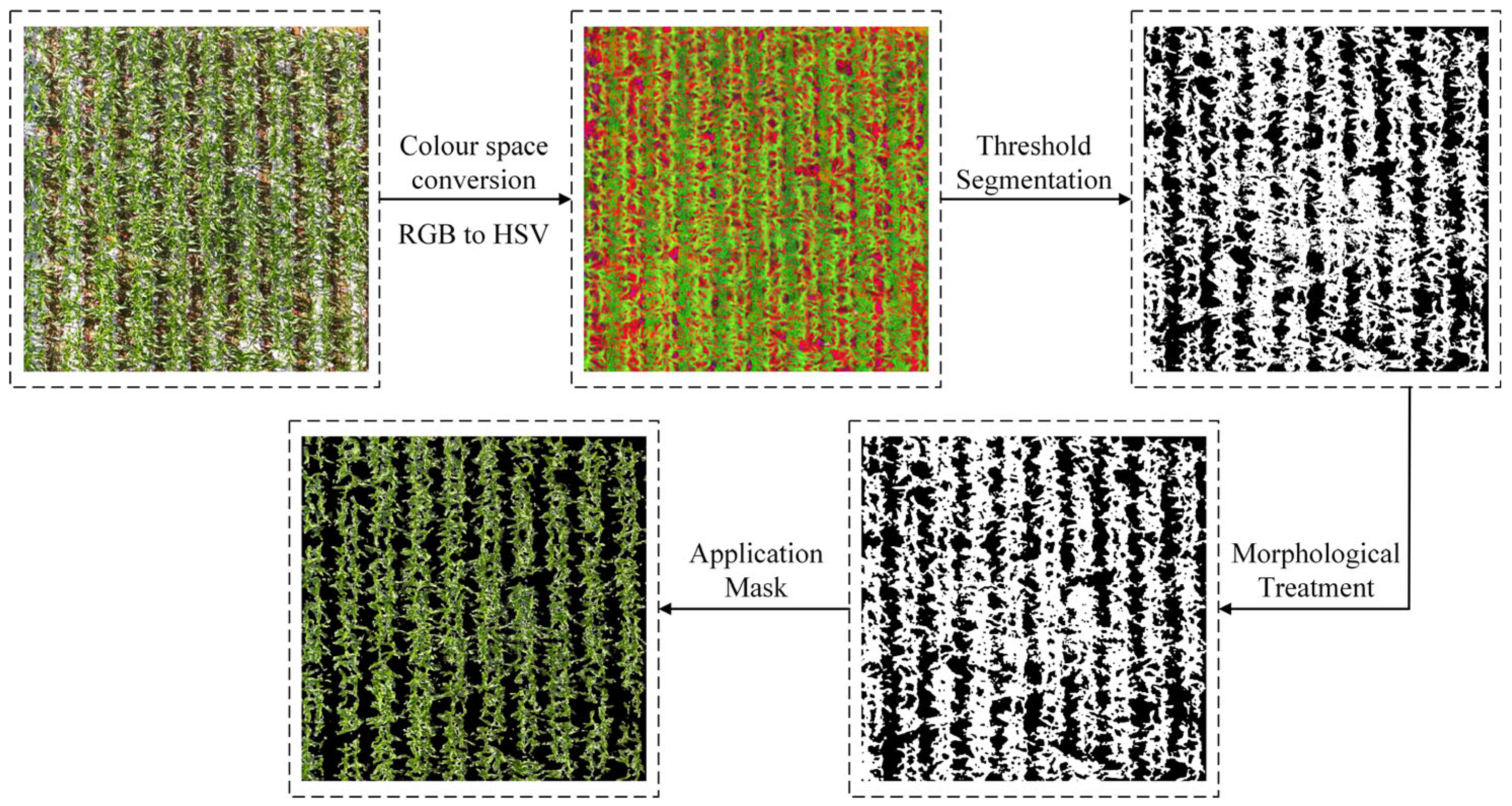
2.4.1. Color and Texture Feature Extraction

We extracted both color and texture features from RGB images. For texture feature extraction, the RGB images were first converted into 8-bit grayscale images. From the grayscale images, smoothness, standard deviation, and third-order moment were calculated. The gray-level co-occurrence matrix (GLCM) was computed in the 45° direction, with a pixel distance of 1, to extract entropy, energy, contrast, uniformity, and correlation.

To improve the accuracy of subsequent analyses and reduce the interference of environmental factors, we employed an image segmentation method based on color thresholding and morphological processing to remove the background from UAV-captured maize canopy images, retaining only the maize plants (Figure 3). First, the original image was converted to the HSV color space to more accurately extract the green areas of the plants. By setting the green low threshold to (35, 40, 40) and the green high threshold to (85, 255, 255), the InRange function was used to extract the maize plant portion, generating a binary mask. Next, morphological operations (opening and closing) were applied to the mask image to remove noise and fill any gaps, thereby accurately extracting the plant regions. Finally, the morphologically processed mask was applied to the original image, using a bitwise AND operation to retain only the plant regions and remove the background. This method does not require complex model training, offering high efficiency and flexibility, making it suitable for image processing under varying lighting and environmental conditions.

We selected 10 color features and 8 texture features as input variables for the model. The parameters and their calculation formulas for each feature are shown in

Table 1. The color and texture features selected for this study.

Title	Features	Formulas	Title	Features	Formulas
R	R		GRD [27]	Green–Red Difference	G-R
G	G		ENT [28]	Entropy	$-{{\displaystyle \sum }}_{i=0}^{L-1}{P}_{i}log\left(P_i\right)$
B	B		ENE [29]	Energy	${{\displaystyle \sum }}_{i=0}^{L-1}{\left[p\left(i,j\right)\right]}^2$
NR	Normalized Red	R/(R + B + G)	COR [30]	Correlation	${\displaystyle \frac{{\sum }_{i=0}^{L-1}{\sum }_{i=0}^{l-1}\left(i-\mu \right)\left(j-\mu \right)p\left(i,j\right)}{{\sigma }^2}}$
NG	Normalized Green	G/(R + B + G)	CON [31]	Contrast	${{\displaystyle \sum }}_{i=0}^{L-1}{{\displaystyle \sum }}_{i=0}^{L-1}{(i-j)}^{2}p\left(i,j\right)$
NB	Normalized Blue	B/(R + B + G)	UNI [32]	Uniformity	${{\displaystyle \sum }}_{i=0}^{L-1}{{\displaystyle \sum }}_{j=0}^{L-1}p{\left(i,j,d,\theta \right)}^2$
NRGD [33]	Normalized Red–Green Difference	${\displaystyle \frac{R-G}{R+G+0.01}}$	THM [34]	Third-Order Moment	${{\displaystyle \sum }}_{i=0}^{L-1}{{\displaystyle \sum }}_{i=0}^{L-1}{\left(i-\mu \right)}^{3}p\left(i,j\right)$
NRBD [33]	Normalized Red–Blue Difference	${\displaystyle \frac{R-B}{R+B+0.01}}$	SMO [35]	Smoothness	${{\displaystyle \sum }}_{i=0}^{L-1}{{\displaystyle \sum }}_{j=0}^{L-1}{\displaystyle \frac{1}{1+{\left(i-j\right)}^2}}p\left(i,j\right)$
GRR [27]	Green/Red Ratio	G/R	STD [36]	Standard Deviation	$\sqrt{{{\displaystyle \sum }}_{i=0}^{L-1}{{\displaystyle \sum }}_{j=0}^{L-1}{\left(i-\mu \right)}^2}p\left(i,j\right)$

Note: L represents the number of gray levels, µ denotes the image mean, p(i,j) indicates the joint probability of gray levels i and j in the image, and σ² represents the variance. P(i,j,d,θ) refers to the gray level covariance matrix of adjacent pixel pairs, where i and j are the pixel gray levels, d is the distance between the pixel pairs, and θ is the direction of the pixel pairs.

.

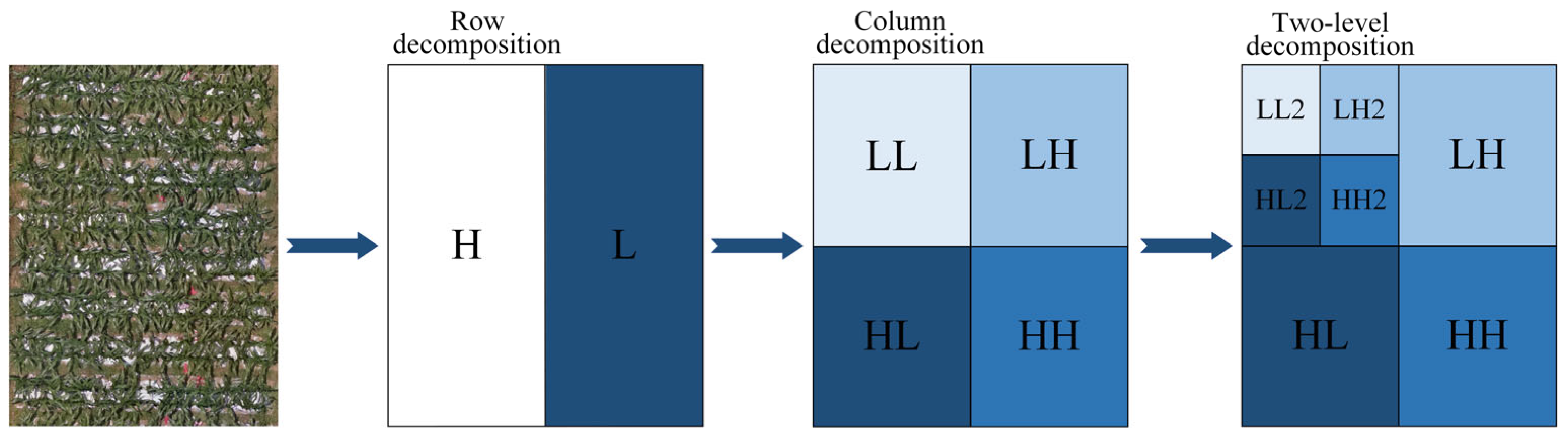
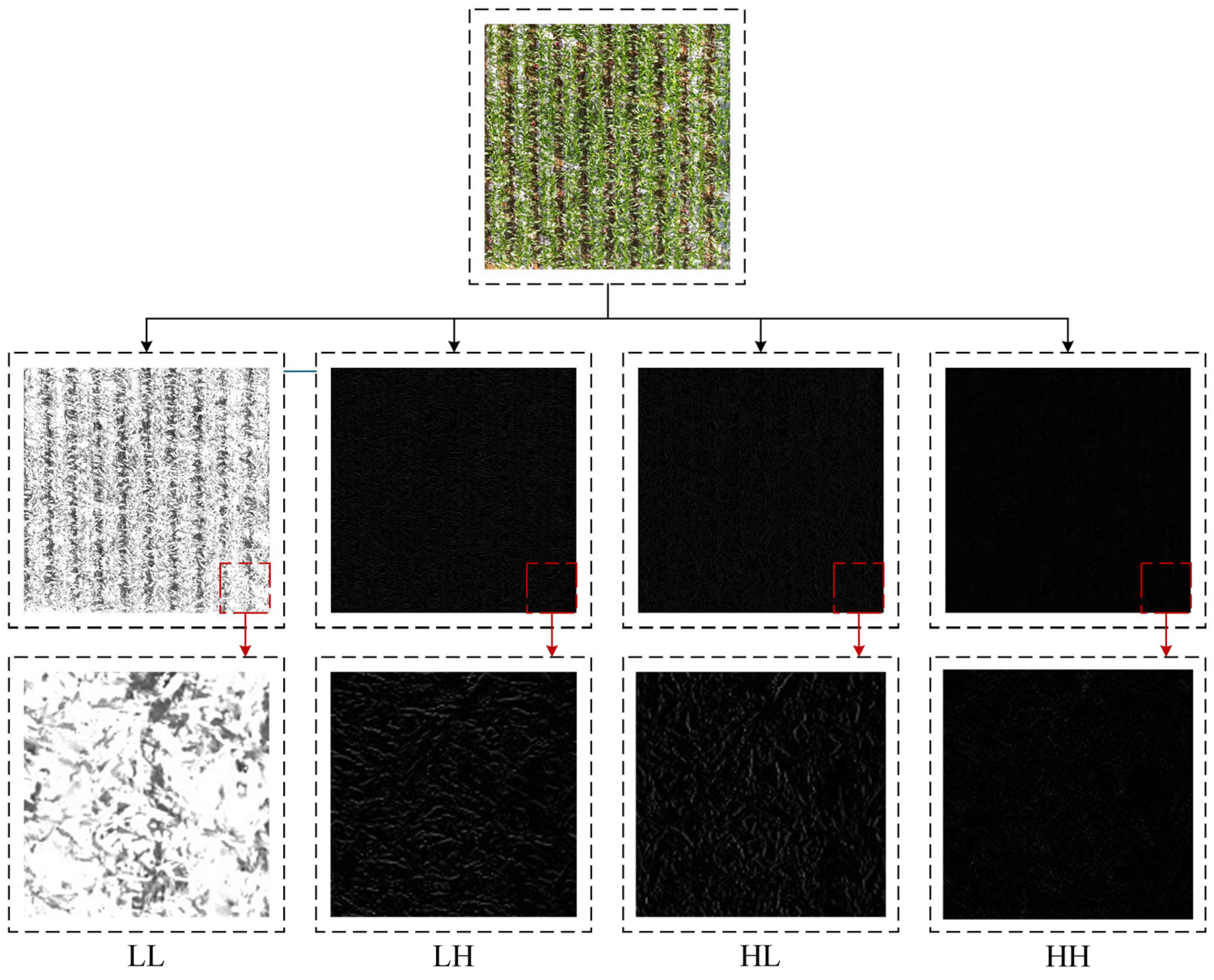
2.4.2. Discrete Wavelet Transform (DWT)

Wavelet transform is a mathematical tool used to decompose signals or images into frequency components at different scales while preserving temporal or spatial information [24]. In this study, the db1 wavelet basis function was selected to perform two-level decomposition of the image (Figure 4). First, the wavelet filter was applied to convolve the image in both horizontal and vertical directions, producing detail coefficients in the horizontal and vertical directions, as well as an approximation coefficient. Subsequently, the detail coefficients were downsampled in both directions to reduce their size while preserving the information. In the next step, the same process was repeated, using the downsampled approximation coefficients for the next level of decomposition. The energy features were calculated by summing the squared wavelet coefficients of the first and second decomposition levels. The following variables were selected as input variables for the model: LL, LH, HL, HH, Level1_energy (L1E), and Level2_energy (L2E).

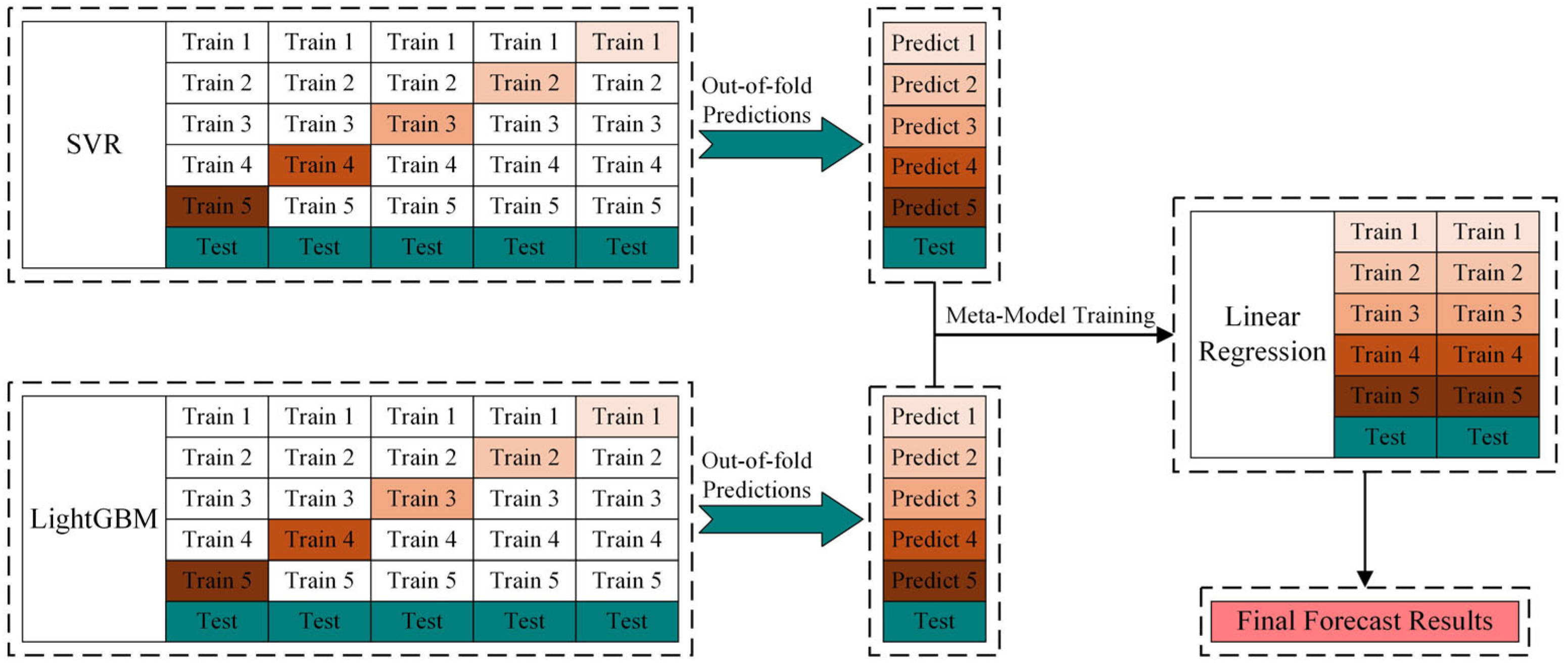
2.4.3. Machine Learning Model Selection

The BP neural network is a model trained with the backpropagation algorithm [37]. This model employs gradient descent optimization through backpropagation, which iteratively updates the weights and biases to reduce the difference between the predicted and actual values [38]. In this study, a custom layer (CustomLayer) was defined as the input layer. During forward pass, the CustomLayer uses the sigmoid function as the activation function, while in the backward pass, it applies an error correction learning rule.

GBDT (Gradient Boosting Decision Tree) is a popular machine learning model used for both regression and classification tasks. It leverages ensemble learning by constructing a series of decision tree models and iteratively improving the model’s performance [39,40]. The GBDT model is resistant to outliers and missing values, performs effectively with high-dimensional sparse data, and is well suited for tackling complex problems [41,42]. In this study, parameter tuning and cross-validation were applied for model fitting on the training set. An exhaustive search was carried out over all possible parameter combinations, and cross-validation was used to assess the performance of each combination, facilitating the automatic selection of the optimal parameter set during the fitting process.

Support Vector Regression (SVR) fits data by identifying an optimal hyperplane in a high-dimensional space, demonstrating strong robustness in handling nonlinear relationships within such spaces [43]. However, the performance of SVR can be influenced by parameter selection, particularly when dealing with complex datasets [44,45]. The SVR model was optimized by conducting a grid search over the key hyperparameters, including the kernel type, regularization parameter (C), and the kernel coefficient (gamma). The kernel used in this study was the radial basis function (RBF) due to its ability to handle nonlinear relationships effectively. LightGBM, a gradient-boosted decision tree model [46], was fine-tuned using random search. Regularization parameters, including L1 and L2 penalties, were adjusted to prevent overfitting, and the minimum child weight and maximum depth parameters were optimized to reduce model complexity. Out-of-fold (OOF) predictions were generated and used as features, which were then input into the meta-model for final prediction. We selected a linear regression model with L2 regularization as the meta-model. During training, five-fold cross-validation divides the dataset into five subsets. Each base model is trained on four subsets and generates OOF predictions on the remaining subset. The OOF predictions from all five folds are then aggregated into a new feature matrix, which serves as input to the meta-model. This ensures the unbiasedness and reliability of the OOF predictions, preventing data leakage into the final model. By learning the combinatorial relationships among these predictions, this approach further enhances the overall predictive performance. This methodology effectively combines the strengths of SVR and LightGBM, better accommodating the characteristics of complex datasets and improving both the predictive accuracy and reliability of the model. The stacking ensemble learning process is shown in Figure 5.

2.4.4. Model Accuracy Verification

In this study, the dataset was divided into training and testing sets in an 8:2 ratio to ensure model training and evaluation accuracy and reliability. The dataset setup is outlined in

Table 2. The dataset setup for this study.

Number	Represent	Alphabet	Represent
1	Jointing stage	R	Non-fusion data
2	Tasseling stage	DR	Fusion data
3	Grouting stage
4	Full birth stage

. After training, the model’s predictions were compared to the actual values in the test set to assess its performance and predictive accuracy. The model was evaluated using three metrics: the coefficient of determination (R²), root mean square error (RMSE), and normalized root mean square error (NRMSE). These metrics were used as follows: R² measures the model’s ability to predict and explain the target variable; the RMSE computes the square root of the average squared differences between the predicted and actual values; and the NRMSE normalizes the RMSE by the target variable’s range, allowing for comparisons between variables with different scales. The formulas for R², RMSE, and NRMSE are given in Equations (1)–(3):

$$\mathrm{RMSE}=\sqrt{{\displaystyle \frac{{\sum }_{i=1}^n{\left(y_p-y_a\right)}^2}{n}}}$$

(1)

$$\mathrm{NRMSE}={\displaystyle \frac{RMSE}{y_{max}-y_{min}}}$$

(2)

$${\mathrm{R}}^2=1-{\displaystyle \frac{{\sum }_{i=1}^n{\left(y_a-y_p\right)}^2}{{\sum }_{i=1}^n{\left(y_a-y_m\right)}^2}}$$

(3)

where n is the number of samples, y_p is the predicted value of the model, y_a is the actual value, y_max and y_min are the maximum and minimum values of the target variable, and y_m denotes the average of the actual values.

3. Results

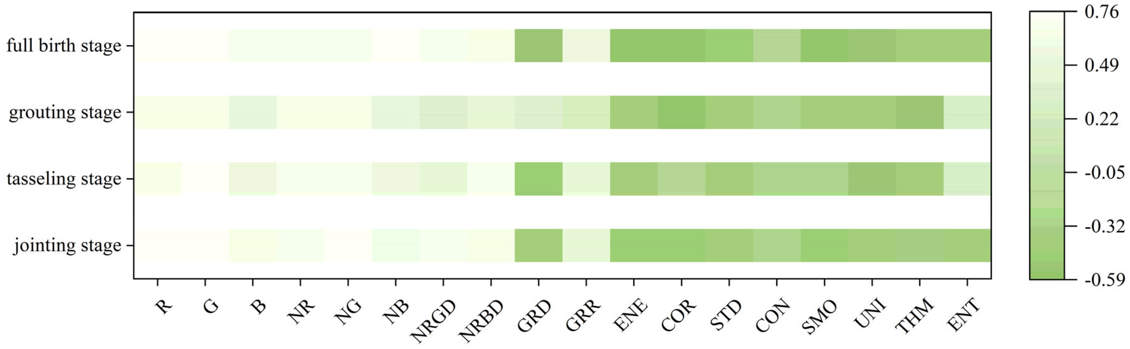
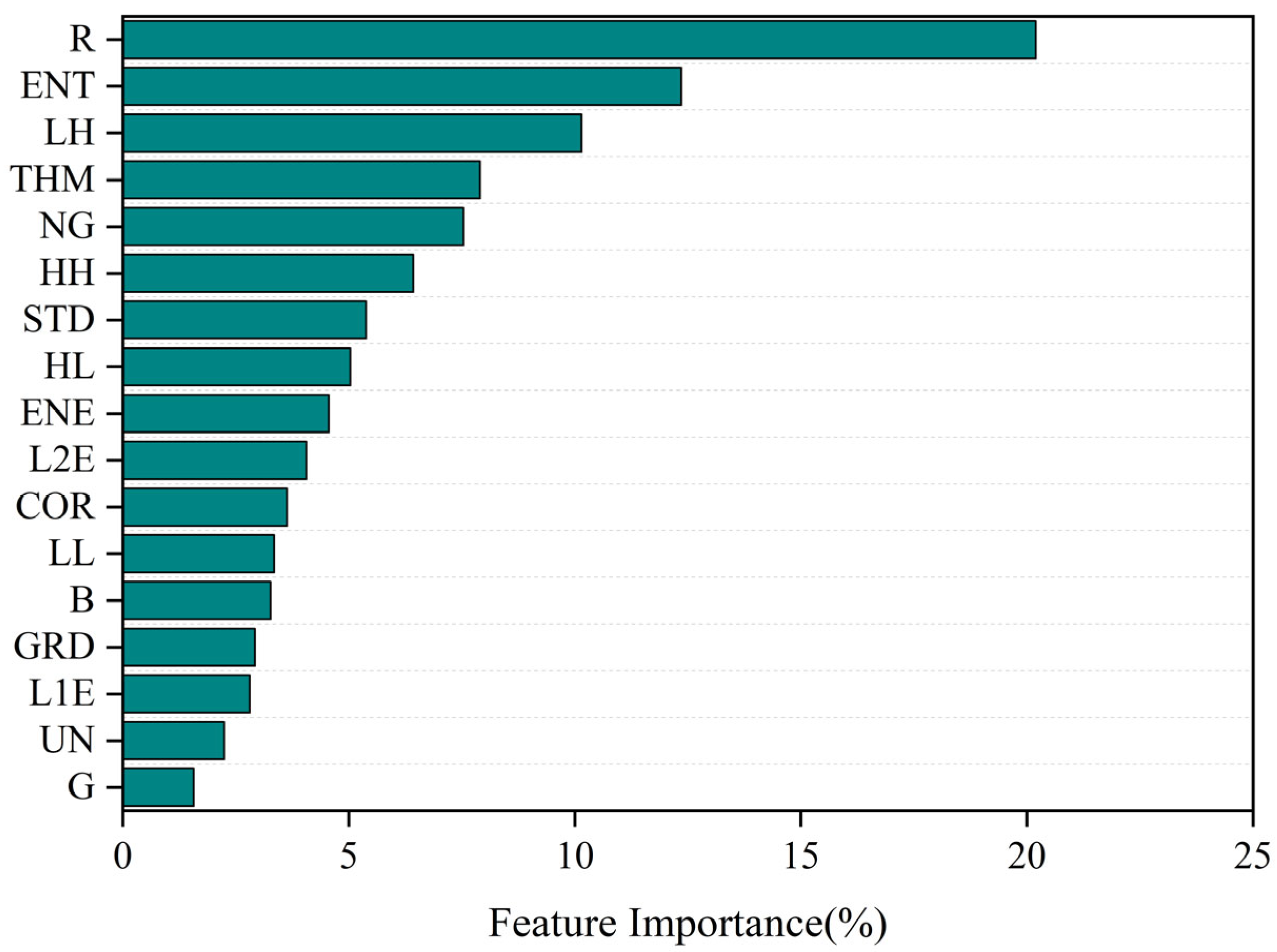
3.1. Correlation Analysis of Chlorophyll Content with Color and Textural Features

A Pearson correlation analysis was conducted to evaluate the relationship between each selected color and texture feature and the maize canopy CHL content individually (Figure 6). The results indicate that NR, NG, R, G, and B showed relatively high correlations with the CHL content during the jointing, tasseling, grouting, and full birth stages. Specifically, the correlation between NR and the CHL content ranged from 0.631 to 0.696, that between NG and the CHL content ranged from 0.667 to 0.755, that between R and the CHL content ranged from 0.631 to 0.725, hat between G and the CHL content ranged from 0.503 to 0.696, and that between B and the CHL content ranged from 0.50 to 0.70. These features effectively monitor the canopy CHL content. Features with absolute correlation coefficients greater than or equal to 0.3 were selected as input variables for the model.

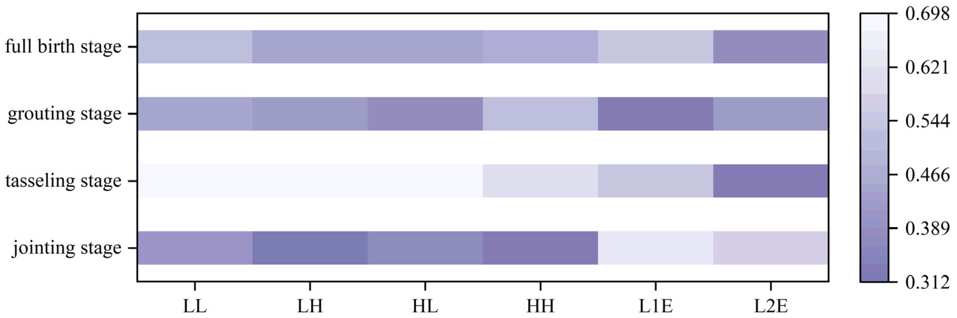
3.2. Correlation Analysis of Chlorophyll Content with Wavelet Characteristics

A Pearson correlation analysis was conducted to evaluate the relationship between each selected wavelet feature and the maize canopy CHL content individually (Figure 7). The results show that LL, LH, HL, HH, Level1_energy (L1E), and Level2_energy (L2E) exhibited strong correlations with the canopy CHL content, with correlation coefficients greater than 0.3. Throughout the maize growing period, L1E demonstrated the strongest correlation with the CHL content (r = 0.531), while L2E showed the weakest correlation (r = 0.377). These findings suggest that using LL, LH, HL, HH, L1E, and L2E to monitor the maize canopy CHL content is effective.

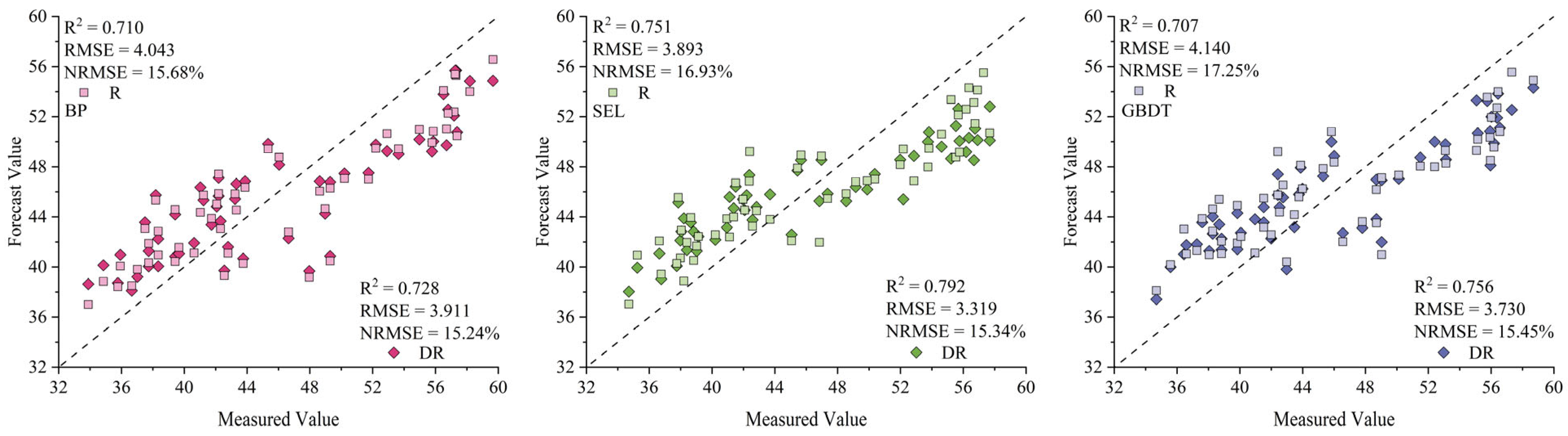
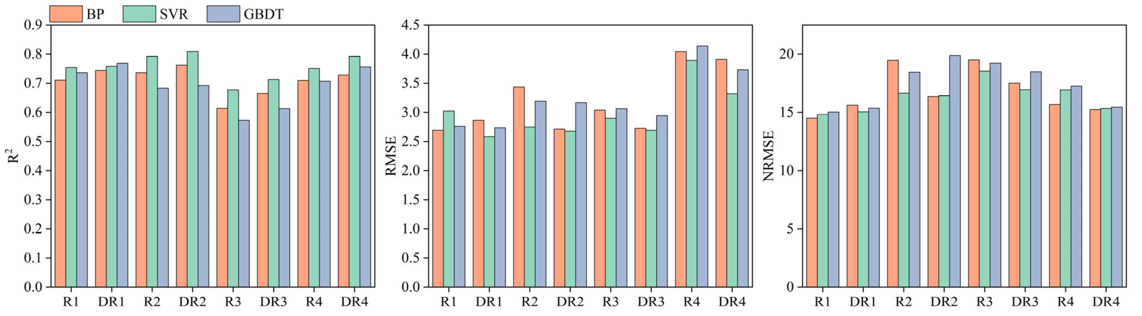
3.3. Inverse Modeling of Maize Canopy Chlorophyll Content

The scatter plots of predicted CHL content values for maize canopies throughout the entire growing period, based on different datasets for the BP, SEL, and GBDT models, are shown in Figure 8. The results indicate that when the maize canopy CHL content is monitored using only UAV-based color and texture features, the R² values of all three models exceed 0.70, with the SEL model achieving the highest accuracy (R² = 0.751, RMSE = 3.893, and NRMSE = 16.93%). The GBDT model demonstrated the lowest accuracy (R² = 0.707, RMSE = 4.140, and NRMSE = 17.25%). When monitoring the maize canopy CHL content using fused data, the accuracy of all three models improved. Among them, the SEL model performed the best, with R² = 0.792, RMSE = 3.319, and NRMSE = 15.34%. Compared to the model using only color and texture features, the R² value increased by 0.041, the RMSE decreased by 0.574, and the NRMSE decreased by 1.59%.

3.4. Comparison of Model Accuracy by Fertility Stage

Figure 9 shows that the DR dataset consistently outperforms the R dataset across all models (SEL, BP, and GBDT) in terms of model fitting and error control. The DR dataset leads to better performance in R², RMSE, and NRMSE, indicating its superior ability to capture data trends and produce more accurate and stable predictions.

The DR dataset achieves higher R² values, reflecting better model fit. For example, the SEL model with DR2 has an R² of 0.809 compared to 0.792 with R². Similar improvements are observed in the BP and GBDT models, where DR data enhance model fitting. The DR dataset also results in lower RMSE values, signifying better prediction accuracy. For instance, the BP model with DR2 has an RMSE of 2.721, which is significantly lower than the 3.437 value obtained with the R2 dataset, with similar trends seen in the SEL and GBDT models. The DR dataset exhibits more stable and consistent performance.

In conclusion, the DR dataset outperforms the R dataset across all evaluation metrics, offering superior model fitting and more reliable predictions. Its higher R² values, lower RMSE, and stable NRMSE make it a more effective choice for model training and future applications. However, the limitations of the DR dataset must be acknowledged. The marginal improvements observed in some models (e.g., RMSE for BP) suggest that wavelet features alone may not fully capture all relevant variations in the canopy structure.

4. Discussion

4.1. Analysis of Feature Fusion Potential

RGB imagery is intuitively interpretable, and the features extracted from the imagery are more easily correlated with the physiological state of plants [14]. RGB imagery can be used not only for monitoring the crop CHL content but also for a range of other applications, including maturity detection, pest and disease monitoring, and the extraction of vegetation information [47,48]. In this study, a remote sensing platform equipped with an RGB sensor on a UAV was used to monitor the canopy CHL content of maize throughout its entire growth cycle. Color features, texture features, and wavelet features were extracted from the RGB imagery to construct separate datasets for color and texture features, as well as a dataset that integrates wavelet features. The BP, SEL, and GBDT algorithms were employed to build monitoring models. The results show that the SEL model provides the best monitoring performance. In comparison to multispectral sensors, RGB sensors are typically more affordable and accessible, making UAVs equipped with RGB sensors highly promising for monitoring the maize canopy CHL content [17]. UAV-based RGB imaging can effectively estimate the black oat canopy height, with an R² value ranging from 0.68 to 0.92 and an RMSE between 0.019 and 0.037 m [49]. It also shows potential in monitoring the coffee production cycle [50]. When combined with the RF algorithm, it can effectively estimate the nitrogen nutrition index (NNI) in rice at different growth stages (R² = 0.88–0.96; RMSE = 0.03–0.07) [51].

Figure 10 presents the results of the feature importance evaluation for each input feature. The results reveal that the red light parameter (R) holds the highest feature importance with a score of 20.19%. The red light parameter (R) typically refers to the characteristic parameter of vegetation when it receives and reflects light in the red spectrum, which is closely related to CHL content [19]. Entropy (ENT) ranks second with a score of 12.35%. This is because entropy is strongly associated with the leaf density and growth condition of maize plants, both of which have a significant impact on the CHL content [28]. The wavelet feature LH ranks third in importance with a score of 10.14%. Wavelet features can reflect the structure and growth conditions of maize plants. When the growth status of plant leaves is good, with a healthy leaf density and structure, the aerial images will show more distinct reflective characteristics, leading to an increase in the wavelet feature LH [24]. The importance of other features ranges from 1% to 8%, indicating that their importance is relatively low.

In conclusion, the red light parameter (R), entropy (ENT), and wavelet feature LH are key features for monitoring the maize canopy CHL content. By assessing the importance of input features, the accuracy and robustness of the monitoring models can be improved, providing valuable guidance for optimizing maize canopy CHL content monitoring methods and improving models in the future.

4.2. Analysis of Discrete Wavelet Transform Potential

Discrete Wavelet Transform (DWT) demonstrates significant potential in agricultural remote sensing and image analysis. Using multi-resolution analysis, DWT decomposes an image into various frequency sub-bands, including the low-frequency sub-band (LL) and high-frequency sub-bands (LH, HL, and HH) [52,53]. The low-frequency sub-band encompasses overall trend information, such as brightness and large-scale structures, while the high-frequency sub-bands capture finer details, including edges and textures [54,55]. DWT effectively reduces noise and enhances image quality by separating high-frequency noise from low-frequency primary features, thereby eliminating sensor noise and preserving critical details [56]. This capability is well suited for agricultural remote sensing applications requiring high image clarity, such as the precise identification of crop canopy structures. DWT exhibits strong compression performance, enabling the reconstruction of most information by storing only a subset of critical coefficients, thereby significantly reducing data storage requirements. Furthermore, DWT can extract texture features in horizontal, vertical, and diagonal directions, facilitating precise crop–background separation or the identification of disease characteristics. DWT also demonstrates potential in multimodal feature fusion. By integrating DWT-derived multi-frequency features with color, spectral, or other texture features, it enhances feature space representation and improves the accuracy of classification or regression models.

In this study, DWT effectively extracted both global and local features, enabling the model to capture overall trend information (e.g., canopy color and light uniformity) as well as local details (e.g., leaf edges and texture variations). The decomposition process is illustrated in Figure 11. Compared to traditional color and texture features, DWT offers distinct advantages. DWT removes noise while retaining useful information, suppressing high-frequency noise effects to enhance data reliability. Multi-frequency features extracted by DWT provide strong discriminative power. The high-frequency sub-bands (LH, HL, and HH) extract details such as edges and textures, effectively highlighting local anomalies like spots or lesions on leaves, which are crucial for early disease detection. In contrast, the low-frequency sub-band (LL) retains key structural information, such as brightness and large-scale patterns, aiding in biomass estimation by reflecting canopy density and light interception. Together, these features provide the model with a comprehensive input for improved performance. The combination of DWT with color and texture features improves the model’s representation capability. DWT’s multi-dimensional feature representation enhances discriminability in a high-dimensional space, maintaining high accuracy with reduced computational complexity.

DWT was applied to RGB images to extract multi-resolution features, supplementing color and texture features. Specifically, DWT decomposes RGB images into wavelet coefficients at different scales and orientations, and energy features are calculated at each decomposition level. These wavelet features are concatenated with color and texture features to form a comprehensive feature set, enhancing feature space representation for machine learning models. The results of this study highlight that DWT significantly improves model inversion accuracy. Compared to models relying solely on color or texture features, those integrating DWT features achieve higher precision and robustness. Consistent with previous studies, the application of DWT in feature extraction demonstrates significant advantages. Tabassum et al. [57] showed that combining DWT with PCA and CNN effectively enhances the quality of feature representation, thereby improving model recognition accuracy. Hasan et al. [58] fused DWT with color histograms to detect and identify apple leaf diseases, achieving an accuracy of 98.63%, highlighting DWT’s potential in plant disease monitoring. Bendjillali et al. [59] extracted facial features using DWT and trained a CNN classifier, confirming DWT’s role in high-precision feature extraction. These studies not only showcase DWT’s extensive applications in image processing but also demonstrate its multi-scale capabilities in capturing both global trends and local details, providing technical support for fine-grained feature extraction in agricultural remote sensing. The methodology of this study aligns with those of the aforementioned research and further validates its potential through successful applications across various fields, demonstrating the broad applicability of DWT in precision agriculture.

4.3. Limitations and Future Prospects

This study provides a novel method for monitoring the chlorophyll content in maize canopies using UAV-based RGB images and Discrete Wavelet Transform features, but it also has certain limitations. First, the reliance on RGB data confines the analysis to the visible spectrum (400–700 nm), limiting its ability to evaluate agronomic variables unrelated to chlorophyll, such as water stress or nutrient deficiencies, which often require information from the near-infrared or thermal spectral range. Second, the robustness of the SEL model has not been validated using multispectral or hyperspectral data. Cross-validation with these advanced sensors could further enhance the model’s reliability and expand its applicability. Lastly, the inherent spatial and temporal variability in field conditions, such as fluctuating light intensities, may affect the results. Therefore, additional measures are needed to account for environmental heterogeneity.

Despite these limitations, this study demonstrates significant potential for practical applications in precision agriculture. The integration of RGB and wavelet features offers a low-cost and scalable method for chlorophyll content monitoring, which can be further extended by incorporating multispectral or hyperspectral data to improve the accuracy of phenotypic monitoring. Additionally, with advanced UAV flight planning and image stitching technologies, this method can be applied to larger farmland environments. The SEL model’s efficiency and accuracy make it highly suitable for real-time crop monitoring systems, providing timely and actionable insights for field management. Furthermore, this study’s findings can be applied to optimize fertilization and irrigation strategies, thereby enhancing crop yields and resource use efficiency.

5. Conclusions

This study constructed maize canopy CHL content monitoring models using BP, SEL, and GBDT algorithms based on two different types of feature datasets. Integrating color features, texture features, and wavelet features as input characteristics can effectively improve the accuracy of maize canopy CHL content monitoring. Compared to using only color and texture features, the models’ R² values increased by 0.018 to 0.049, the RMSE decreased by 0.132 to 0.574, and the NRMSE decreased by 0.44% to 1.8%.

Among the models, the SEL-based canopy CHL content monitoring model outperformed the BP and GBDT models in both accuracy and performance. Although using only color and texture feature data as input also yielded good monitoring results, integrating wavelet feature data resulted in even better monitoring precision.

In conclusion, the maize canopy CHL content monitoring model that integrates wavelet transform features with SEL effectively and accurately estimates the CHL content in an efficient and intuitive manner. This study offers valuable technical support for precision field management. However, due to the limitations of this study, the effect of feature fusion can be assessed more comprehensively in the future by expanding the sample size or introducing other metrics.

References

1. Kasim, N.; Sawut, R.; Abliz, A.; Qingdong, S.; Maihmuti, B.; Yalkun, A.; Kahaer, Y. Estimation of the relative chlorophyll content in spring wheat Based on an optimized spectral index. Photogramm. Eng. Remote Sens. 2018, 84, 801–811. [Google Scholar] [CrossRef]
2. Li, J.; Wijewardane, N.K.; Ge, Y.; Shi, Y. Improved chlorophyll and water content estimations at leaf level with a hybrid radiative transfer and machine learning model. Comput. Electron. Agric. 2023, 206, 107669. [Google Scholar] [CrossRef]
3. Liu, Y.; Hatou, K.; Aihara, T.; Kurose, S.; Akiyama, T.; Kohno, Y.; Lu, S.; Omasa, K. A robust vegetation index based on different UAV RGB images to estimate SPAD values of naked barley leaves. Remote Sens. 2021, 13, 686. [Google Scholar] [CrossRef]
4. Steele, M.R.; Gitelson, A.A.; Rundquist, D.C. A comparison of two techniques for nondestructive measurement of chlorophyll content in grapevine leaves. Agron. J. 2008, 100, 779–782. [Google Scholar] [CrossRef]
5. Teshome, F.T.; Bayabil, H.K.; Hoogenboom, G.; Schaffer, B.; Singh, A.; Ampatzidis, Y. Unmanned aerial vehicle (UAV) imaging and machine learning applications for plant phenotyping. Comput. Electron. Agric. 2023, 212, 108064. [Google Scholar] [CrossRef]
6. Colomina, I.; Molina, P. Unmanned aerial systems for photogrammetry and remote sensing: A review. ISPRS J. Photogramm. Remote Sens. 2014, 92, 79–97. [Google Scholar] [CrossRef]
7. Xie, Q.; Dash, J.; Huete, A.; Jiang, A.; Yin, G.; Ding, Y.; Peng, D.; Hall, C.C.; Brown, L.; Shi, Y. Retrieval of crop biophysical parameters from Sentinel-2 remote sensing imagery. Int. J. Appl. Earth Obs. Geoinf. 2019, 80, 187–195. [Google Scholar] [CrossRef]
8. Candiago, S.; Remondino, F.; De Giglio, M.; Dubbini, M.; Gattelli, M. Evaluating multispectral images and vegetation indices for precision farming applications from UAV images. Remote Sens. 2015, 7, 4026–4047. [Google Scholar] [CrossRef]
9. Gevaert, C.M.; Suomalainen, J.; Tang, J.; Kooistra, L. Generation of spectral–temporal response surfaces by combining multispectral satellite and hyperspectral UAV imagery for precision agriculture applications. IEEE J. Sel. Top. Appl. Earth Obs. Remote Sens. 2015, 8, 3140–3146. [Google Scholar] [CrossRef]
10. Hunt, E.R., Jr.; Daughtry, C.S. What good are unmanned aircraft systems for agricultural remote sensing and precision agriculture? Int. J. Remote Sens. 2018, 39, 5345–5376. [Google Scholar] [CrossRef]
11. Sun, Q.; Sun, L.; Shu, M.; Gu, X.; Yang, G.; Zhou, L. Monitoring maize lodging grades via unmanned aerial vehicle multispectral image. Plant Phenomics 2019, 2019, 5704154. [Google Scholar] [CrossRef]
12. Gautam, D.; Ostendorf, B.; Pagay, V. Estimation of grapevine crop coefficient using a multispectral camera on an unmanned aerial vehicle. Remote Sens. 2021, 13, 2639. [Google Scholar] [CrossRef]
13. Njane, S.N.; Tsuda, S.; van Marrewijk, B.M.; Polder, G.; Katayama, K.; Tsuji, H. Effect of varying UAV height on the precise estimation of potato crop growth. Front. Plant Sci. 2023, 14, 1233349. [Google Scholar] [CrossRef] [PubMed]
14. Li, B.; Xu, X.; Han, J.; Zhang, L.; Bian, C.; Jin, L.; Liu, J. The estimation of crop emergence in potatoes by UAV RGB imagery. Plant Methods 2019, 15, 15. [Google Scholar] [CrossRef]
15. Zhang, Y.; Li, S.; Wang, S.; Wang, X.; Duan, H. Distributed bearing-based formation maneuver control of fixed-wing UAVs by finite-time orientation estimation. Aerosp. Sci. Technol. 2023, 136, 108241. [Google Scholar] [CrossRef]
16. Zhao, J.; Gao, F.; Jia, W.; Yuan, W.; Jin, W. Integrated sensing and communications for UAV communications with jittering effect. IEEE Wirel. Commun. Lett. 2023, 12, 758–762. [Google Scholar] [CrossRef]
17. Istiak, M.A.; Syeed, M.M.; Hossain, M.S.; Uddin, M.F.; Hasan, M.; Khan, R.H.; Azad, N.S. Adoption of Unmanned Aerial Vehicle (UAV) imagery in agricultural management: A systematic literature review. Ecol. Inform. 2023, 78, 102305. [Google Scholar] [CrossRef]
18. Delavarpour, N.; Koparan, C.; Nowatzki, J.; Bajwa, S.; Sun, X. A technical study on UAV characteristics for precision agriculture applications and associated practical challenges. Remote Sens. 2021, 13, 1204. [Google Scholar] [CrossRef]
19. Kou, J.; Duan, L.; Yin, C.; Ma, L.; Chen, X.; Gao, P.; Lv, X. Predicting leaf nitrogen content in cotton with UAV RGB images. Sustainability 2022, 14, 9259. [Google Scholar] [CrossRef]
20. Aiazzi, B.; Alparone, L.; Baronti, S.; Garzelli, A. Context-driven fusion of high spatial and spectral resolution images based on oversampled multiresolution analysis. IEEE Trans. Geosci. Remote Sens. 2002, 40, 2300–2312. [Google Scholar] [CrossRef]
21. Shi, W.; Zhu, C.; Zhu, C.; Yang, X. Multi-band wavelet for fusing SPOT panchromatic and multispectral images. Photogramm. Eng. Remote Sens. 2003, 69, 513–520. [Google Scholar] [CrossRef]
22. Liu, H.; Sun, H.; Li, M.; Iida, M. Application of color featuring and deep learning in maize plant detection. Remote Sens. 2020, 12, 2229. [Google Scholar] [CrossRef]
23. Cheng, T.; Riaño, D.; Ustin, S.L. Detecting diurnal and seasonal variation in canopy water content of nut tree orchards from airborne imaging spectroscopy data using continuous wavelet analysis. Remote Sens. Environ. 2014, 143, 39–53. [Google Scholar] [CrossRef]
24. Xu, X.; Li, Z.; Yang, X.; Yang, G.; Teng, C.; Zhu, H.; Liu, S. Predicting leaf chlorophyll content and its nonuniform vertical distribution of summer maize by using a radiation transfer model. J. Appl. Remote Sens. 2019, 13, 034505. [Google Scholar] [CrossRef]
25. Zhai, W.; Li, C.; Cheng, Q.; Ding, F.; Chen, Z. Exploring multisource feature fusion and stacking ensemble learning for accurate estimation of maize chlorophyll content using unmanned aerial vehicle remote sensing. Remote Sens. 2023, 15, 3454. [Google Scholar] [CrossRef]
26. Hnizil, O.; Baidani, A.; Khlila, I.; Nsarellah, N.; Laamari, A.; Amamou, A. Integrating NDVI, SPAD, and Canopy Temperature for Strategic Nitrogen and Seeding Rate Management to Enhance Yield, Quality, and Sustainability in Wheat Cultivation. Plants 2024, 13, 1574. [Google Scholar] [CrossRef] [PubMed]
27. Zhu, X.; Yang, Q.; Chen, X.; Ding, Z. An approach for joint estimation of grassland leaf area index and leaf chlorophyll content from UAV hyperspectral data. Remote Sens. 2023, 15, 2525. [Google Scholar] [CrossRef]
28. Zhao, X.; Li, Y.; Chen, Y.; Qiao, X.; Qian, W. Water chlorophyll a estimation using UAV-based multispectral data and machine learning. Drones 2022, 7, 2. [Google Scholar] [CrossRef]
29. Zhou, L.; Nie, C.; Su, T.; Xu, X.; Song, Y.; Yin, D.; Liu, S.; Liu, Y.; Bai, Y.; Jia, X. Evaluating the canopy chlorophyll density of maize at the whole growth stage based on multi-scale UAV image feature fusion and machine learning methods. Agriculture 2023, 13, 895. [Google Scholar] [CrossRef]
30. Yin, H.; Huang, W.; Li, F.; Yang, H.; Li, Y.; Hu, Y.; Yu, K. Multi-temporal UAV imaging-based mapping of chlorophyll content in potato crop. PFG–J. Photogramm. Remote Sens. Geoinf. Sci. 2023, 91, 91–106. [Google Scholar] [CrossRef]
31. Ban, S.; Liu, W.; Tian, M.; Wang, Q.; Yuan, T.; Chang, Q.; Li, L. Rice leaf chlorophyll content estimation using UAV-based spectral images in different regions. Agronomy 2022, 12, 2832. [Google Scholar] [CrossRef]
32. Kandhway, P. A novel adaptive contextual information-based 2D-histogram for image thresholding. Expert Syst. Appl. 2024, 238, 122026. [Google Scholar] [CrossRef]
33. Woebbecke, D.M.; Meyer, G.E.; Von Bargen, K.; Mortensen, D.A. Color indices for weed identification under various soil, residue, and lighting conditions. Trans. ASAE 1995, 38, 259–269. [Google Scholar] [CrossRef]
34. Qian, B.; Shao, W.; Gao, R.; Zheng, W.; Hua, D.; Li, H. The extended digital image correlation based on intensity change model. Measurement 2023, 221, 113416. [Google Scholar] [CrossRef]
35. Huang, Y.; Ma, Q.; Wu, X.; Li, H.; Xu, K.; Ji, G.; Qian, F.; Li, L.; Huang, Q.; Long, Y. Estimation of chlorophyll content in Brassica napus based on unmanned aerial vehicle images. Oil Crop Sci. 2022, 7, 149–155. [Google Scholar] [CrossRef]
36. Gamon, J.; Surfus, J. Assessing leaf pigment content and activity with a reflectometer. New Phytol. 1999, 143, 105–117. [Google Scholar] [CrossRef]
37. Dong, Y.; Fu, Z.; Peng, Y.; Zheng, Y.; Yan, H.; Li, X. Precision fertilization method of field crops based on the Wavelet-BP neural network in China. J. Clean. Prod. 2020, 246, 118735. [Google Scholar] [CrossRef]
38. Zhao, Z.; Feng, G.; Zhang, J. The simplified hybrid model based on BP to predict the reference crop evapotranspiration in Southwest China. PLoS ONE 2022, 17, e0269746. [Google Scholar] [CrossRef] [PubMed]
39. Li, L.; Dai, S.; Cao, Z.; Hong, J.; Jiang, S.; Yang, K. Using improved gradient-boosted decision tree algorithm based on Kalman filter (GBDT-KF) in time series prediction. J. Supercomput. 2020, 76, 6887–6900. [Google Scholar] [CrossRef]
40. Zhang, Z.; Jung, C. GBDT-MO: Gradient-boosted decision trees for multiple outputs. IEEE Trans. Neural Netw. Learn. Syst. 2020, 32, 3156–3167. [Google Scholar] [CrossRef] [PubMed]
41. Yao, H.; Huang, Y.; Wei, Y.; Zhong, W.; Wen, K. Retrieval of chlorophyll-a concentrations in the coastal waters of the Beibu Gulf in Guangxi using a gradient-boosting decision tree model. Appl. Sci. 2021, 11, 7855. [Google Scholar] [CrossRef]
42. Yuan, Z.; Ye, Y.; Wei, L.; Yang, X.; Huang, C. Study on the optimization of hyperspectral characteristic bands combined with monitoring and visualization of pepper leaf SPAD value. Sensors 2021, 22, 183. [Google Scholar] [CrossRef] [PubMed]
43. Li, Y.; Sun, H.; Yan, W.; Zhang, X. Multi-output parameter-insensitive kernel twin SVR model. Neural Netw. 2020, 121, 276–293. [Google Scholar] [CrossRef] [PubMed]
44. Sun, Y.; Ding, S.; Zhang, Z.; Jia, W. An improved grid search algorithm to optimize SVR for prediction. Soft Comput. 2021, 25, 5633–5644. [Google Scholar] [CrossRef]
45. Verma, B.; Prasad, R.; Srivastava, P.K.; Yadav, S.A.; Singh, P.; Singh, R. Investigation of optimal vegetation indices for retrieval of leaf chlorophyll and leaf area index using enhanced learning algorithms. Comput. Electron. Agric. 2022, 192, 106581. [Google Scholar] [CrossRef]
46. Yang, H.; Hu, Y.; Zheng, Z.; Qiao, Y.; Zhang, K.; Guo, T.; Chen, J. Estimation of potato chlorophyll content from UAV multispectral images with stacking ensemble algorithm. Agronomy 2022, 12, 2318. [Google Scholar] [CrossRef]
47. Liu, T.; Li, R.; Zhong, X.; Jiang, M.; Jin, X.; Zhou, P.; Liu, S.; Sun, C.; Guo, W. Estimates of rice lodging using indices derived from UAV visible and thermal infrared images. Agric. For. Meteorol. 2018, 252, 144–154. [Google Scholar] [CrossRef]
48. Sorbelli, F.B.; Palazzetti, L.; Pinotti, C.M. YOLO-based detection of Halyomorpha halys in orchards using RGB cameras and drones. Comput. Electron. Agric. 2023, 213, 108228. [Google Scholar] [CrossRef]
49. Acorsi, M.G.; das Dores Abati Miranda, F.; Martello, M.; Smaniotto, D.A.; Sartor, L.R. Estimating biomass of black oat using UAV-based RGB imaging. Agronomy 2019, 9, 344. [Google Scholar] [CrossRef]
50. Barbosa, B.D.S.; Araújo e Silva Ferraz, G.; Mendes dos Santos, L.; Santana, L.S.; Bedin Marin, D.; Rossi, G.; Conti, L. Application of rgb images obtained by uav in coffee farming. Remote Sens. 2021, 13, 2397. [Google Scholar] [CrossRef]
51. Qiu, Z.; Ma, F.; Li, Z.; Xu, X.; Ge, H.; Du, C. Estimation of nitrogen nutrition index in rice from UAV RGB images coupled with machine learning algorithms. Comput. Electron. Agric. 2021, 189, 106421. [Google Scholar] [CrossRef]
52. Zhang, Y.; Hong, G. An IHS and wavelet integrated approach to improve pan-sharpening visual quality of natural colour IKONOS and QuickBird images. Inf. Fusion 2005, 6, 225–234. [Google Scholar] [CrossRef]
53. Yocky, D.A. Image merging and data fusion by means of the discrete two-dimensional wavelet transform. J. Opt. Soc. Am. A 1995, 12, 1834–1841. [Google Scholar] [CrossRef]
54. Zhou, J.; Civco, D.L.; Silander, J.A. A wavelet transform method to merge Landsat TM and SPOT panchromatic data. Int. J. Remote Sens. 1998, 19, 743–757. [Google Scholar] [CrossRef]
55. Ranchin, T.; Wald, L. Fusion of high spatial and spectral resolution images: The ARSIS concept and its implementation. Photogramm. Eng. Remote Sens. 2000, 66, 49–61. [Google Scholar]
56. Vaidya, S.P.; Mouli, P.C. Robust digital color image watermarking based on compressive sensing and DWT. Multimed. Tools Appl. 2024, 83, 3357–3371. [Google Scholar] [CrossRef]
57. Tabassum, F.; Islam, M.I.; Khan, R.T.; Amin, M.R. Human face recognition with combination of DWT and machine learning. J. King Saud Univ.-Comput. Inf. Sci. 2022, 34, 546–556. [Google Scholar] [CrossRef]
58. Hasan, S.; Jahan, S.; Islam, M.I. Disease detection of apple leaf with combination of color segmentation and modified DWT. J. King Saud Univ.-Comput. Inf. Sci. 2022, 34, 7212–7224. [Google Scholar] [CrossRef]
59. Bendjillali, R.I.; Beladgham, M.; Merit, K.; Taleb-Ahmed, A. Improved facial expression recognition based on DWT feature for deep CNN. Electronics 2019, 8, 324. [Google Scholar] [CrossRef]
Figure 1. Overview of experimental site location and density settings. Note: D1–D3 represent different densities: 5.7, 6.3, and 6.9 plants/m2.
Agronomy 15 00212 g001
Figure 2. Flow chart for remote sensing data processing.
Agronomy 15 00212 g002
Figure 3. Workflow for removing image background.
Agronomy 15 00212 g003
Figure 4. The decomposition procedure of the image. Note: H denotes a high-pass filter, L denotes a low-pass filter, LL denotes the proximate feature, HL denotes the longitudinal edge feature, LH denotes the lateral edge feature, and HH denotes the diagonal feature.
Agronomy 15 00212 g004
Figure 5. Stacking ensemble learning implementation process integrating SVR and LightGBM.
Agronomy 15 00212 g005
Figure 6. Heatmap of correlation between color and texture features and CHL content.
Agronomy 15 00212 g006
Figure 7. Heat map of correlation between wavelet features and CHL content.
Agronomy 15 00212 g007
Figure 8. Scatterplot of predicted chlorophyll content of BP, SEL, and GBDT models based on different data.
Agronomy 15 00212 g008
Figure 9. Distribution of R2, RMSE, and NRMSE at different growth stages of maize.
Agronomy 15 00212 g009
Figure 10. Ranking the importance of color, texture, and wavelet features.
Agronomy 15 00212 g010
Figure 11. Schematic diagram of discrete wavelet decomposition.
Agronomy 15 00212 g011