Early Detection of Verticillium Wilt in Cotton by Using Hyperspectral Imaging Combined with Recurrence Plots

Abstract

Cotton is susceptible to Verticillium wilt (VW) during its growth. Early and accurate detection of VW can facilitate targeted pesticide treatment and reduce the potential spread of the disease. However, accurately detecting VW in cotton before symptoms appear (the asymptomatic period) after infection by Verticillium dahliae remains challenging. This study proposes an early detection method for cotton wilt disease using hyperspectral imaging and recurrence plots (RP) combined with machine learning techniques. First, spectral curves were collected and analyzed under three conditions of cotton plants: healthy, asymptomatic, and symptomatic. Then, the one-dimensional spectral curve was transformed into two-dimensional recurrence plots to enhance the detail differences in the original spectral curve of cotton plants in various states. Hyperspectral recurrence plots contain rich texture information; fifteen texture features were extracted from the spectral recurrence plots using the Gray-Level Gradient Co-occurrence Matrix (GLGCM). Eleven of these texture features showed a strong correlation with the class labels of the cotton plants. In order to reduce redundant information between features, principal component analysis (PCA) was used to extract the first five principal components, which explained 99.02% of the information from the 11 features. The final principal component dataset was then input into KNN, SVM, ELM, and XGBoost classifiers to assess the accuracy of early detection of VW in cotton. The results showed that the XGBoost model, based on the first five principal components obtained from the texture features, achieved accuracy, precision, recall, and F1-score of 96.3%, 95.6%, 96%, and 95.8%, demonstrating a high classification capability. The results of this study confirm the feasibility of converting spectral curves into recurrence plots and extracting image texture features for the accurate identification of VW in cotton during the asymptomatic period. This method also provides a new strategy for early disease detection of cotton and other plants in the future.

1. Introduction

Cotton plants are highly susceptible to diseases during their growth, significantly impacting their yield and quality, with an average annual yield loss of 15% to 20%. Among these diseases, Verticillium wilt (VW) is the most severe and widespread, often referred to as the “cancer of cotton” [1]. Severe cases of Verticillium wilt in cotton can lead to significant yield reductions or even total crop failure, resulting in substantial economic and social losses [2]. Currently, the task of preventing and controlling VW is extremely challenging, and the detection and management of its spread have emerged as key research focal points.

The pathogenic mechanism of Verticillium wilt involves Verticillium dahliae secreting toxins that degrade the cell walls of crop roots, leading to extensive colonization of the plant’s xylem [3]. By the time visible symptoms appear, Verticillium dahliae has already extensively parasitized the crop, causing irreversible damage [4]. Therefore, detecting Verticillium wilt before it parasitizes extensively on plant xylem (in the asymptomatic stage) is beneficial for its prevention and control. Traditional detection methods primarily rely on visual inspection to confirm the type and severity of the disease, which are often inaccurate and delayed. Laboratory fungal culturing for detecting Verticillium dahliae can achieve accurate early diagnosis; however, this method requires destructive sampling and is time-consuming, labor-intensive, and expensive [5]. Therefore, there is a need for more effective methods for the rapid and non-destructive detection of Verticillium wilt.

Spectral technology has been employed to accurately monitor the physiological changes associated with plant stress [6]. Under disease stress, plants experience changes in internal physiological responses and phenotypic traits, including physiological indicators, which in turn alter their optical properties and external morphology [7,8]. Jing et al. [9] conducted a correlation analysis between the severity of Verticillium wilt in individual cotton leaves and the original first derivative spectral reflectance, along with hyperspectral characteristic parameters, to develop a model for predicting disease severity. The results indicated that the spectral reflectance in the visible and shortwave infrared bands increased with the severity of the disease. Chen et al. [10] applied hyperspectral remote sensing to monitor the photosynthetic parameters of cotton leaves under Verticillium wilt stress. They obtained spectral data from 207 leaf samples of varying disease severity at different stages, focusing on the 350–500 nm spectral range, to extract physiological parameters related to Verticillium wilt. Zhang et al. [11] analyzed the canopy spectral data of infected cotton plants and combined the support vector machine (SVM) model with genetic algorithm (GA), grid search (GS), particle swarm optimization (PSO), Gray Wolf optimizer (GWO), and other optimization algorithms to establish a cotton verticillium classification model. The result showed that accuracy, macro accuracy, macro recall rate, and macro F1-score indexes are 91.2%, 92.02%, 91.2%, and 91.16%, respectively. Lu et al. [12] proposed a new method for cotton Verticillium wilt recognition based on the fusion of spectral and image features and established a classification model using support vector machine (SVM) and backpropagation neural network (BPNN). By spectral and image-fused features, the SG-MN-SPA-FF-BPNN model obtained the best performance with a classification accuracy of 98.99%. However, most previous studies have primarily monitored Verticillium wilt when symptoms are already present, with relatively little research focusing on detecting the disease during the asymptomatic stage.

In recent years, some studies have begun to focus on the spectral detection of leaf pathogens in the asymptomatic stage [13,14,15]. Riefolo et al. [16] used hyperspectral data analysis as a tool to diagnose Xylella fastidiosa in the asymptomatic leaves of olive plants, to reduce the infection risk for the surrounding plants. The result showed an unsupervised classification, using only spectral data, was able to discriminate the infected plants at a very early stage of infection. Cao et al. [17] tested the feasibility of detecting early asymptomatic infection of the rice BLB disease based on hyperspectral imaging and spectral dilated convolution 3-dimensional convolutional neural network (SDC-3DCNN), providing sufficient support for early warning and rice disease prevention. Li et al. [18] extracted wavelet coefficients and vegetation indices from the hyperspectral data and selected sensitive spectral features for cotton VW. By leveraging these selected features, they developed machine learning models to assess the severity of cotton VW at the canopy scale.

During the asymptomatic stage, the secretions of Verticillium dahliae trigger the host’s immune response and disrupt the hormonal balance of the plant [19], leading to vessel occlusion and oxidative stress [20,21]. These changes ultimately alter the structure and composition of the leaves, providing a basis for the spectral detection of Verticillium wilt during the asymptomatic period. However, during the asymptomatic stage, subtle changes in the internal structure and photosynthetic capacity of the leaves are challenging to detect using raw spectral data. There may be overlapping features in the raw spectra, making it difficult to achieve early detection using these data alone. Gao et al. [22] showed that in the early stage of grape leaf curl disease, the raw spectra of healthy leaves and virus-infected leaves highly overlapped, which led to difficulties in early detection of the disease using the raw spectrum. Signal imaging technology can convert a one-dimensional curve into a two-dimensional image and magnify the detail differences in the curve. Yang et al. [23] utilized continuous wavelet transform (CWT) to process the hyperspectral curve and selected the optimal wavelet features from the images. Finally, the support vector machine, logistic regression, and K-Nearest Neighbors (KNNs) were used to construct the models for detecting VW in asymptomatic leaves; the average accuracy of the logistic regression model based on wavelet features was as high as 90.62%. Recurrence plots (RPs) are also a method used to visualize and analyze time series or dynamic systems. They convert time series data into a graphical representation, capable of capturing subtle differences in curve features. This representation method has been widely applied in fault diagnosis analysis and electrocardiogram signal recognition [24,25,26,27]. Zhang et al. [28] converted hyperspectral curves of lamb meat with different adulteration ratios into recurrence plots to amplify subtle differences between the spectral curves. This approach demonstrated great potential in classifying adulterated lamb meat, achieving classification accuracies of 100.00%, 100.00%, and 99.95% across three datasets. Yang et al. [29] converted impact signals from dropped kiwifruit into recurrence plots, which amplified the differences in impact signals among kiwifruit of varying firmness levels. The results showed that the classification accuracy based on recurrence plots and a CNN model was 98.34%. Currently, the application of recurrence plot-based spectral imaging methods for the early detection of Verticillium wilt in cotton is relatively limited.

Therefore, exploring the potential of converting spectral curves into two-dimensional recurrence plots for the early detection of Verticillium wilt in cotton will be both intriguing and valuable. The objectives of this study include: (1) analyzing the response of spectral curves under three conditions of cotton: healthy, asymptomatic, and symptomatic; (2) converting the spectral curves from these three conditions into recurrence plots, extracting and analyzing the corresponding image texture features, and performing feature selection; and (3) evaluating the accuracy of identifying Verticillium wilt using the extracted recurrence plot texture features with KNN, SVM, ELM, and XGBoost classification algorithms and realizing the early detection of asymptomatic Verticillium wilt of cotton.

2. Materials and Methods

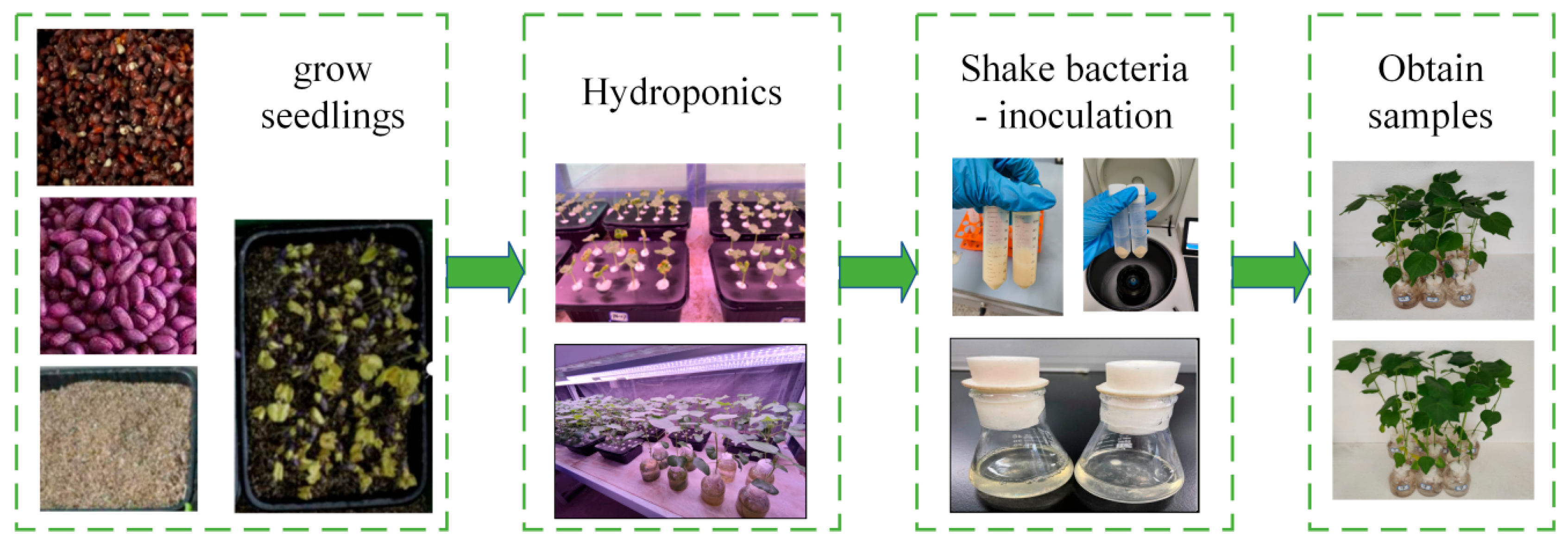
2.1. Experimental Sample Acquisition

Two cotton varieties with different levels of resistance to Verticillium wilt were selected, including Xinluzao 76 and Xinluzao 1. The selection of cotton varieties with different resistance levels to Verticillium wilt is mainly based on the resistance mechanism of cotton to Verticillium wilt, so as to increase the diversity of data samples and cover cotton with different resistance levels to Verticillium wilt. The seeds of Xinluzao 76, classified as a Verticillium wilt-tolerant variety, were purchased from the Shihezi Seed Wholesale Market and approved by the Crop Variety Approval Committee of the Xinjiang Uygur Autonomous Region in 2016. Xinluzao 1, known for its lower resistance to Verticillium wilt, was provided by the Plant Pathology Laboratory of the College of Agriculture at Shihezi University.

To minimize the impact of external factors and more precisely control cotton growth, this study adopted a hydroponic cultivation method. Hydroponic cultivation offers superior control over nutrient supply and growth conditions such as temperature, humidity, and light, providing optimal growth environments for cotton while simultaneously minimizing soil-borne pests and diseases to further ensure its healthy development. The hydroponic setup was located in the greenhouse laboratory of the College of Agriculture at Shihezi University (latitude 44°18′58″ N, longitude 86°3′34″ E). The temperature, humidity, and light conditions in the greenhouse can be controlled; light for 16 h and darkness for 8 h, the average temperature in the greenhouse is about 25 °C, and the average relative humidity is about 30%. The hydroponic nutrient solution used was the standard Hoagland solution, a commonly used standard nutrient formula for soilless cultivation. It mainly includes K₂SO₄ (607 mg/L), NH₄H₂PO₄ (115 mg/L), MgSO₄ (493 mg/L), and Ca(NO₃)₂ (945 mg/L). The growth conditions of the cotton plants were monitored daily, and detailed experimental records were maintained.

To improve the success rate of Verticillium wilt inoculation, a root soaking method was employed. The Verticillium dahliae strain was provided by the Plant Pathology Laboratory at the College of Agriculture, Shihezi University. Inoculation was performed when the cotton plants reached the four-leaf stage, following recommendations from agricultural experts for optimal timing. The roots of the cotton plants designated for infection were soaked in the prepared Verticillium dahliae spore suspension (density 1 × 10⁷ conidia/mL) for 30 min. After soaking, the inoculated plants were immediately returned to the hydroponic containers, completing the inoculation process. The specific experimental process is shown in Figure 1.

2.2. Hyperspectral Image Acquisition and Preprocessing

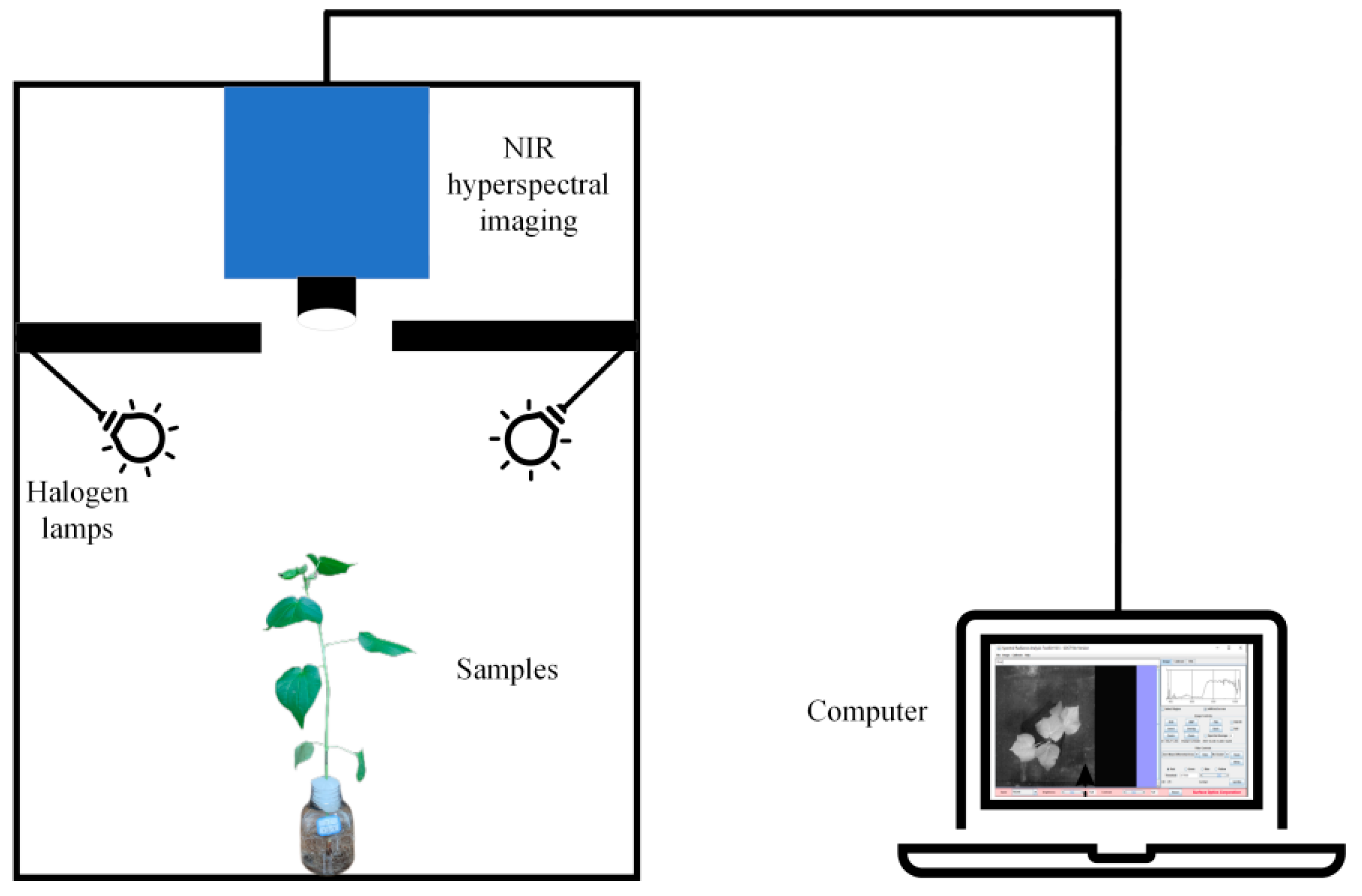
2.2.1. Hyperspectral Image Acquisition

After inoculating the cotton plants with the Verticillium wilt pathogen, a continuous imaging strategy was employed to capture the earliest possible samples of Verticillium wilt. We selected 40 cotton plants with good growth and development from each of the two varieties and collected them continuously for 15 days, obtaining a total of 1200 hyperspectral images. The day of inoculation with Verticillium dahliae was recorded as ‘day 0’. To obtain data during the asymptomatic phase of VW infection in a timely manner, this study conducted data acquisition 24 h after inoculation in the greenhouse. On the 9th day of infection, the leaves on the infected cotton plant had already shown symptoms, manifested as yellowing, softening, and the appearance of pale yellow lesions. The state of each cotton plant was monitored and identified using the expertise of agricultural specialists and the national standard of GB/T 22101.5-2009 [30]. The sample taken on the day symptoms first appeared was designated as an early-stage Verticillium wilt sample. The hyperspectral imaging system used in the experiment consists of two main modules: hardware and software. The hardware components include the SOC710 SWIR hyperspectral imager (Surface Optics Corporation, San Diego, CA, USA), a light source, a height adjustment device, a diffuse reflectance reference panel, a dark box, and transmission cables. The NIR hyperspectral imaging system (SOC 710SWIR) has a spectral wavelength range of 915–1699 nm, a spectral resolution of 2.7 nm, and the number of bands is 288. The software components consist of the HyperScanner (2.0) tool for hyperspectral image data acquisition and the SRAnal710 tool for data analysis. The specific structure of the system is illustrated in Figure 2.

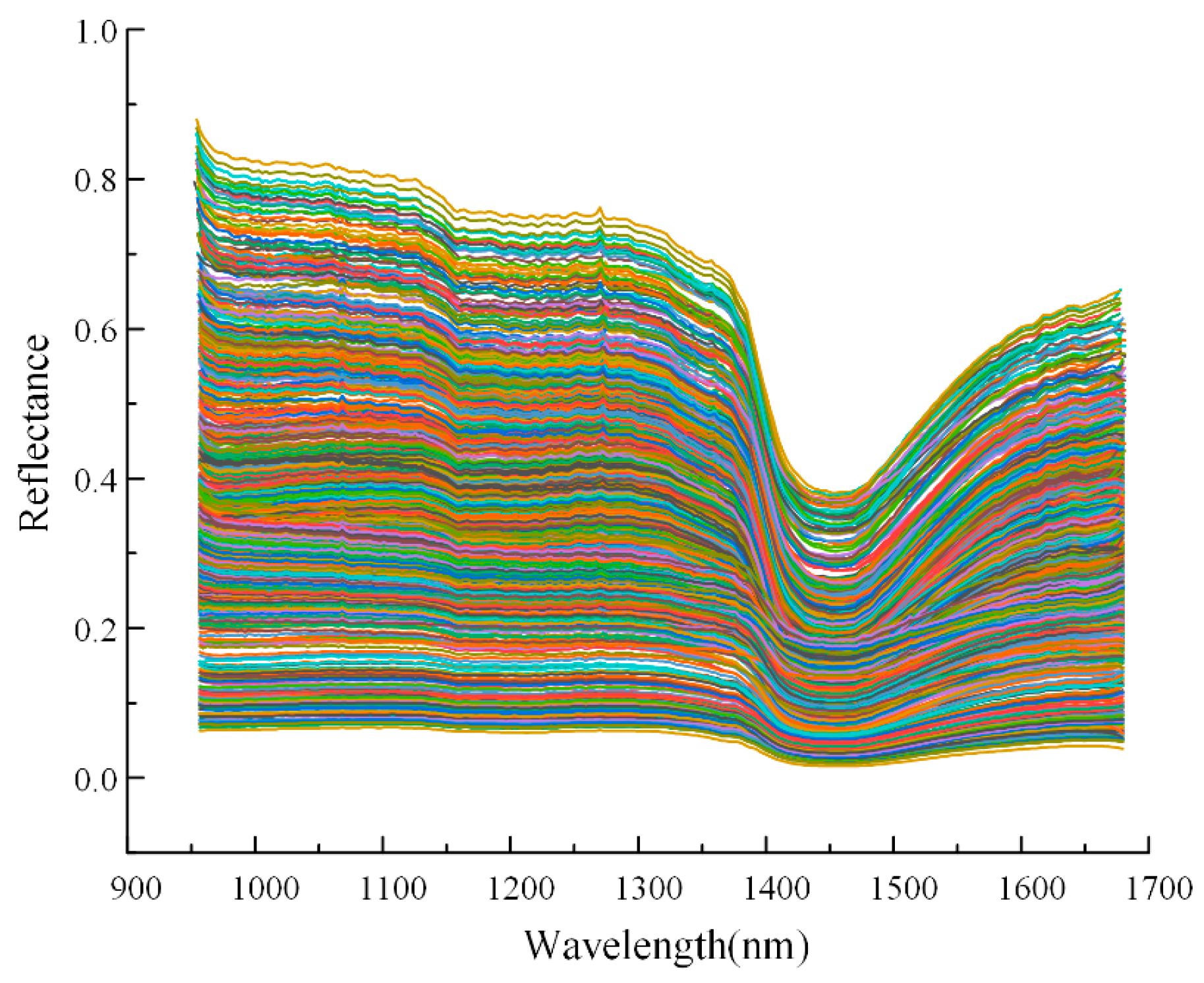
2.2.2. Hyperspectral Image Preprocessing

The entire cotton plant was designated as the Region of Interest (ROI). A threshold value of 0.02 was set to differentiate the foreground ROI (cotton plant) from the background. A binary mask was created accordingly, where 0 represented the background and 1 represented the foreground cotton plant. This mask was then applied to the complete hyperspectral image to obtain a background-removed hyperspectral image. Subsequently, the mean pixel value was calculated for each channel, initially obtaining the background-removed cotton spectral curve (Figure 3). Due to the presence of dark current in the charge-coupled device (CCD) camera and uneven illumination intensity across different wavelengths—resulting in significant noise in some bands with weaker light intensity—it was necessary to perform black-and-white calibration to remove noise caused by environmental factors and dark current. The calibration process was conducted using the following Equation (1):

$${\mathrm{I}}_{\mathrm{calibrated}}={\displaystyle \frac{{\mathrm{I}}_{\mathrm{raw}}-{ \mathrm{I}}_{\mathrm{dark}}}{{\mathrm{I}}_{\mathrm{white}}-{ \mathrm{I}}_{\mathrm{dark}}}}$$

(1)

where ${\mathrm{I}}_{\mathrm{calibrated}}$ is the calibrated image; ${\mathrm{I}}_{\mathrm{raw}}$ is the raw hyperspectral image; ${\mathrm{I}}_{\mathrm{dark}}$ is the dark reflectance image with 0% reflectance; and ${\mathrm{I}}_{\mathrm{white}}$ is the white reflectance image with approximately 100% reflectance.

2.3. Recurrence Plots (RP)

Recurrence plots (RPs) are graphical tools that utilize nonlinear dynamic analysis methods to reflect the behavior of systems in the phase space of one-dimensional signal time series. Eckmann et al. [31] indicated that recurrence plots could analyze the periodicity, chaotic nature, and non-smoothness of time series. They represent time–domain information using phase space trajectories and convert important feature information into visual images. Seo D. et al. [25] demonstrated that recurrence plots could detect dynamic changes and feature information within time series data.

Therefore, this study focuses on the hyperspectral time series curves of cotton plants under different Verticillium wilt conditions. The one-dimensional spectral signal time series are reconstructed into a high-dimensional phase space and converted into two-dimensional images. The specific steps are as follows:

Phase space reconstruction of the original time series using Takens embedding theorem is obtained:

$${\mathrm{X}}_{\mathrm{i}}=\left\{{\mathrm{x}}_{\mathrm{i}}{, \mathrm{x}}_{\mathrm{i}+\mathsf{\tau }}{, \dots , \mathrm{x}}_{\mathrm{i}+(\mathrm{d}-1)\mathsf{\tau }}\right\} (\mathrm{i}=1, 2, \dots , \mathrm{N})$$

(2)

where τ is the delay time and d is the embedding dimension, N = n − (d − 1)τ. The corresponding delay time and embedding dimension are obtained by the mutual information analysis method with the false nearest neighbor algorithm as τ = 2 and d = 4.

The distance between any two vectors in Euclidean space is as follows:

$${\mathrm{d}}_{\mathrm{ij}}=\parallel {\mathrm{X}}_{\mathrm{i}}-{\mathrm{Y}}_{\mathrm{j}}\parallel$$

(3)

Depending on the chosen distance threshold ε, the RP is represented as:

$${\mathrm{R}}_{\mathrm{ij}}=\mathsf{\Theta }\left(\mathsf{\epsilon }-{\mathrm{d}}_{\mathrm{ij}}\right)$$

(4)

where Θ(.) is the Heaviside function, ε is usually set to 10% of the standard deviation of the original time series.

2.4. Image Texture Feature

2.4.1. Image Texture Feature Extraction

Texture is an important piece of information that can reflect the structural arrangement of the image surface. Different texture features have different descriptive abilities and emphases. By combining multiple features, image texture information can be described more comprehensively and accurately. Grayscale conversion is performed on the hyperspectral curve RP images of cotton plants in three different states. Subsequently, the Gray-Level Gradient Co-occurrence Matrix (GLGCM) was employed to capture the second-order statistics of grayscale and gradient information in the grayscale recurrence plot images [32]. The program in MATLAB R2018b was used to extract a total of 15 texture features (

Table 1. Textural features of GLGCM and the corresponding formulas.

Texture Features	Calculating Formula	Texture Features	Calculating Formula
Small gradient dominance	$T_1={\displaystyle \frac{{\sum }_{x=0}^{L_f-1} {{\sum }_{y=0}^{L_g-1}\widehat{H}(x,y)/(y+1)}^2}{{\sum }_{x=0}^{L_f-1}{\sum }_{y=0}^{L_g-1}\widehat{H}(x,y)}}$	Gradient variance	$T_9={\left\{{\displaystyle \sum _{y=0}^{L_g-1}}{\left(y-T_7\right)}^2{\displaystyle \sum _{x=0}^{L_f-1}}\widehat{H}(x,y)\right\}}^{\frac{1}{2}}$
Large gradient dominance	$T_2={\displaystyle \frac{{\sum }_{x=0}^{L_f-1}{{\sum }_{y=0}^{L_g-1}\widehat{H}(x,y)y}^2}{{\sum }_{x=0}^{L_f-1}{\sum }_{y=0}^{L_g-1}\widehat{H}(x,y)}}$	Correlation	$T_{10}={\displaystyle \sum _{x=0}^{L_f-1}}{\displaystyle \sum _{y=0}^{L_g-1}}\left(x-T_6\right)\left(y-T_7\right)\widehat{H}(x,y)$
Gray asymmetry	$T_3={\displaystyle \frac{{\sum }_{x=0}^{L_f-1}{[{\sum }_{y=0}^{L_g-1}\widehat{H}(x,y)]}^2}{{\sum }_{x=0}^{L_f-1}{\sum }_{y=0}^{L_g-1}\widehat{H}(x,y)}}$	Gray entropy	$T_{11}=-{\displaystyle \sum _{x=0}^{L_f-1}}{\displaystyle \sum _{y=0}^{L_g-1}}\widehat{H}(x,y)\mathrm{l}\mathrm{o}\mathrm{g}{\displaystyle \sum _{y=0}^{L_g-1}}\widehat{H}(x,y)$
Gradient asymmetry	$T_4={\displaystyle \frac{{\sum }_{y=0}^{L_g-1}{[{\sum }_{x=0}^{L_f-1}\widehat{H}(x,y)]}^2}{{\sum }_{x=0}^{L_f-1}{\sum }_{y=0}^{L_g-1}\widehat{H}(x,y)}}$	Gradient entropy	$T_{12}=-{\displaystyle \sum _{y=0}^{L_g-1}}{\displaystyle \sum _{x=0}^{L_f-1}}\widehat{H}(x,y)\mathrm{l}\mathrm{o}\mathrm{g}{\displaystyle \sum _{x=0}^{L_f-1}}\widehat{H}(x,y)$
Energy	$T_5={\displaystyle \sum _{x=0}^{L_f-1}}{\displaystyle \sum _{y=0}^{L_g-1}}\widehat{H^2}(x,y)$	Mixing entropy	$T_{13}=-{\displaystyle \sum _{x=0}^{L_f-1}}{\displaystyle \sum _{y=0}^{L_g-1}}\widehat{H}(x,y)\mathrm{l}\mathrm{o}\mathrm{g}\widehat{H}(x,y)$
Gray mean	$T_6={\displaystyle \sum _{x=0}^{L_f-1}}x{\displaystyle \sum _{y=0}^{L_g-1}}\widehat{H}(x,y)$	Inertia	$T_{14}={\displaystyle \sum _{x=0}^{L_f-1}}{\displaystyle \sum _{y=0}^{L_g-1}}(x-y{)}^2\widehat{H}(x,y)$
Gradient mean	$T_7={\displaystyle \sum _{y=0}^{L_g-1}}y{\displaystyle \sum _{x=0}^{L_f-1}}\widehat{H}(x,y)$	Inverse difference moment	$T_{15}={\displaystyle \sum _{x=0}^{L_f-1}}{\displaystyle \sum _{y=0}^{L_g-1}}{\displaystyle \frac{H(x,y)}{1+(x-y{)}^2}}$
Gray variance	$T_8={\left\{{\displaystyle \sum _{x=0}^{L_f-1}}{\left(x-T_6\right)}^2{\displaystyle \sum _{y=0}^{L_g-1}}\widehat{H}(x,y)\right\}}^{\frac{1}{2}}$

Note: x is the gray-level value; Lf is the number of gray levels; y is the gradient value; and Lg is the number of gradient levels. Element H(x, y) is defined as the total number of pixels of the normalized grayscale image and its normalized gradient image. $\hat{\mathrm{H}}$(x, y) is the normalized GLGCM, and make the sum of its elements equal to 1.

). Different GLGCM feature parameters characterize the texture distribution of recurrence plot images from various perspectives. Specifically, small gradient dominance, large gradient dominance, gray asymmetry, and gradient asymmetry describe the distribution of grayscale and gradient within the image texture. Energy reflects the uniformity and coarseness of the texture distribution. Gray mean and gradient mean represent the concentration of grayscale and gradient in the image texture. Gray variance and gradient variance indicate the periodicity of texture variations. Correlation describes the similarity of local grayscale and gradient along rows or columns in the image. Gray entropy, gradient entropy, and mixing entropy characterize the complexity or heterogeneity of the texture. Inertia moment represents the clarity and the prominence of grooves in the texture, while inverse difference moment reflects the homogeneity and regularity of the texture.

2.4.2. Image Texture Feature Analysis

Three categories of labels were established: healthy cotton plants, asymptomatic plants, and symptomatic plants. Pearson correlation analysis was performed to assess the correlation between the 15 texture features and these labels, identifying the texture features moderately or strongly associated with the occurrence of cotton Verticillium wilt. To eliminate redundant information among the features, principal component analysis (PCA) was used to extract the principal components (PCs).

2.5. Model Building Method

Based on the Kennard–Stone algorithm, 1200 selected cotton plant samples were randomly divided into training and test sets in a 3:1 ratio. Four classification models, namely KNN, SVM, ELM, and XGBoost, were employed for the classification of healthy, asymptomatic, and symptomatic samples.

2.5.1. K-Nearest Neighbors (KNNs)

K-Nearest Neighbors (KNNs) is a classical supervised classification modeling method. It first calculates the distance between the points in the known category dataset and the current data point, then selects the K data points with the smallest distance to the current point. The category with the highest frequency among these K data points is taken as the classification result for the current data point [33]. The Euclidean distance method is used for distance measurement, with distance weights set to equal distance. Five-fold cross-validation is employed to prevent model overfitting, and through multiple tests, K is set to 5.

2.5.2. Support Vector Machine (SVM)

Support vector machine (SVM) introduces a kernel function to map low-dimensional space vectors to a high-dimensional space and constructs a linear decision function in the high-dimensional space to achieve nonlinear decision-making in the original space [34]. In this study, the Radial Basis Function (RBF) was chosen as the kernel function. The hyperparameters, penalty coefficient (c) and kernel function parameter (g), were optimized using the grid search algorithm and were determined to be c = 2 and g = 1.5.

2.5.3. Extreme Learning Machines (ELMs)

Extreme Learning Machines (ELMs) is a learning algorithm used for single-hidden-layer feedforward neural networks [35]. Unlike traditional neural network training methods such as backpropagation, ELM is characterized by fast learning. During the training process, ELM randomly initializes the input weights and hidden layer biases without adjustment. The output weights are calculated by minimizing the error in the output layer, thus completing the training. The optimal number of hidden layer neurons, determined to be n = 12, was tested by varying the number of hidden layer neurons within the range of 2–30 based on the minimum classification error.

2.5.4. eXtreme Gradient Boosting (XGBoost)

eXtreme Gradient Boosting (XGBoost) is an improved Boosting ensemble learning algorithm based on Gradient Boosting trees. It uses decision trees as weak learners, iteratively adding new decision trees until a stopping criterion is met and then taking the weighted sum of the fitting results of multiple decision trees to obtain the final classification result [36]. The hyperparameters, learning rate (r), maximum depth of the decision trees (m), and the number of decision trees (n) were optimized using the grid search algorithm and were determined to be r = 0.1, m = 23, and n = 110. High parameter values can increase the complexity of the model, potentially leading to overfitting; low parameter values can increase training time and make it difficult to capture features.

2.6. Model Evaluation

To accurately evaluate the classification performance of the early detection models for cotton Verticillium wilt, this study uses overall accuracy, precision, recall, and F1-score as classification evaluation metrics to assess the performance of the KNN, SVM, ELM, and XGBoost classification models. The formulas are shown in Equations (5)–(8).

$$\mathrm{Overall} \mathrm{Accuracy}={\displaystyle \frac{\mathrm{TP}+\mathrm{TN}}{\mathrm{TP}+\mathrm{FP}+\mathrm{TN}+\mathrm{FN}}}$$

(5)

$$\mathrm{Precision}={\displaystyle \frac{\mathrm{TP}}{\mathrm{TP}+\mathrm{FP}}}$$

(6)

$$\mathrm{Recall}={\displaystyle \frac{\mathrm{TP}}{\mathrm{TP}+\mathrm{FN}}}$$

(7)

$${\mathrm{F}}_1 \mathrm{Score}={\displaystyle \frac{2 \times \mathrm{Recall} \times \mathrm{Precision}}{\mathrm{Recall}+\mathrm{Precision}}}$$

(8)

In these formulas, TP (true positive) represents the number of true positive samples, FP (false positive) represents the number of false positive samples, TN (true negative) represents the number of true negative samples, and FN (false negative) represents the number of false negative samples.

3. Results and Discussion

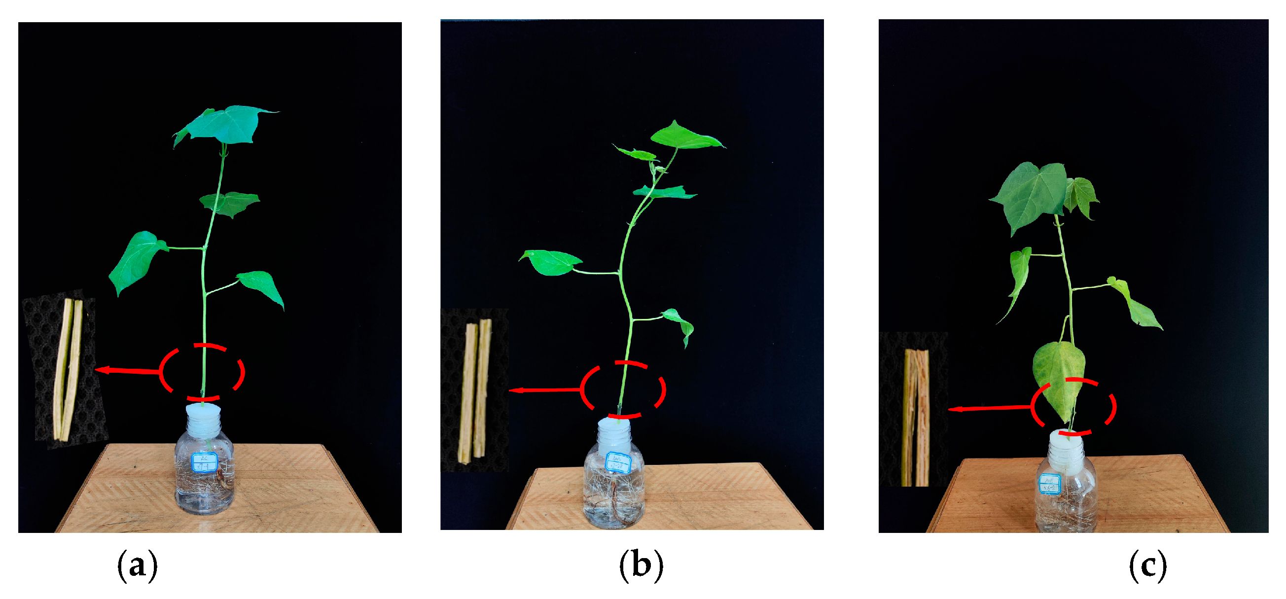
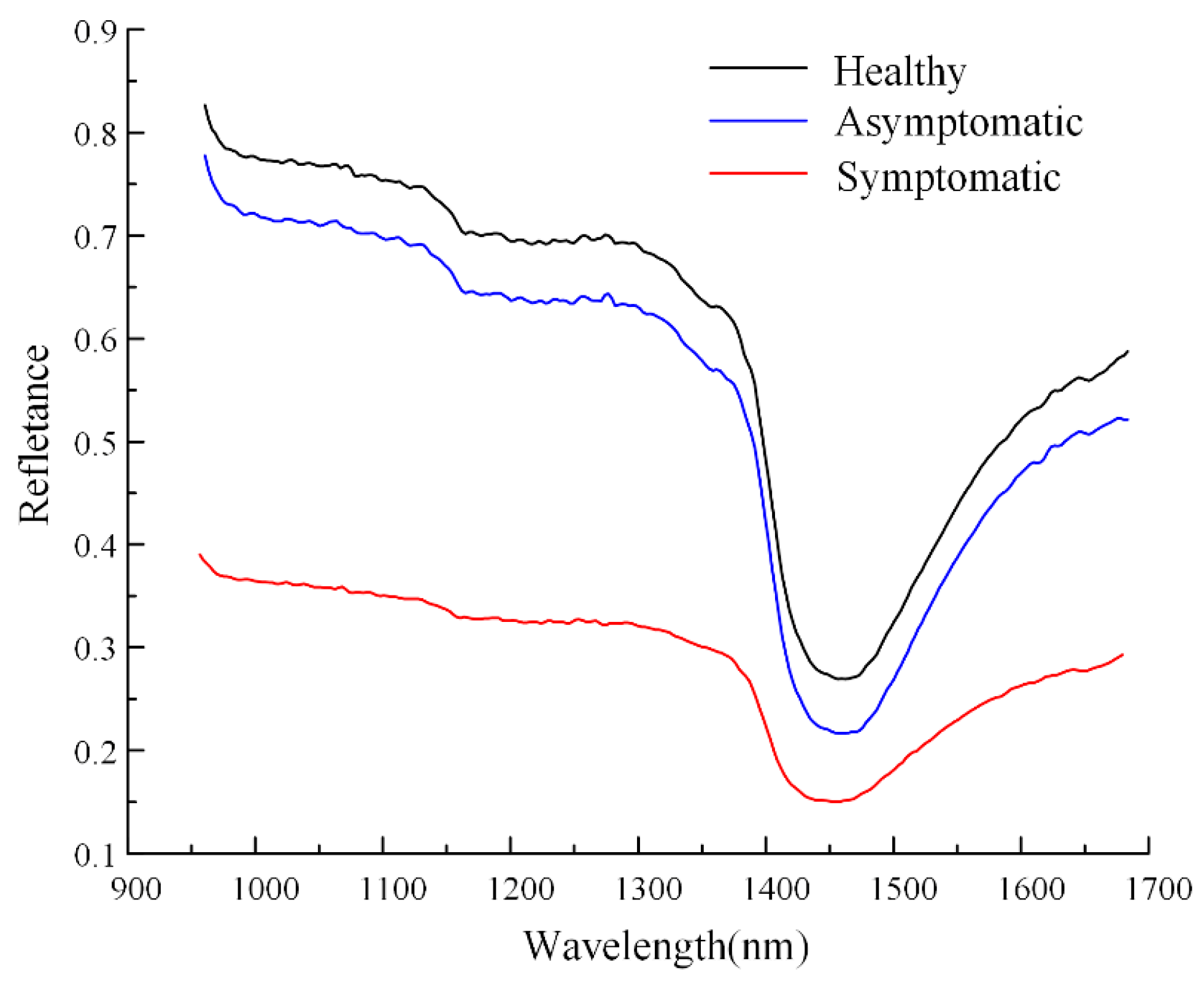
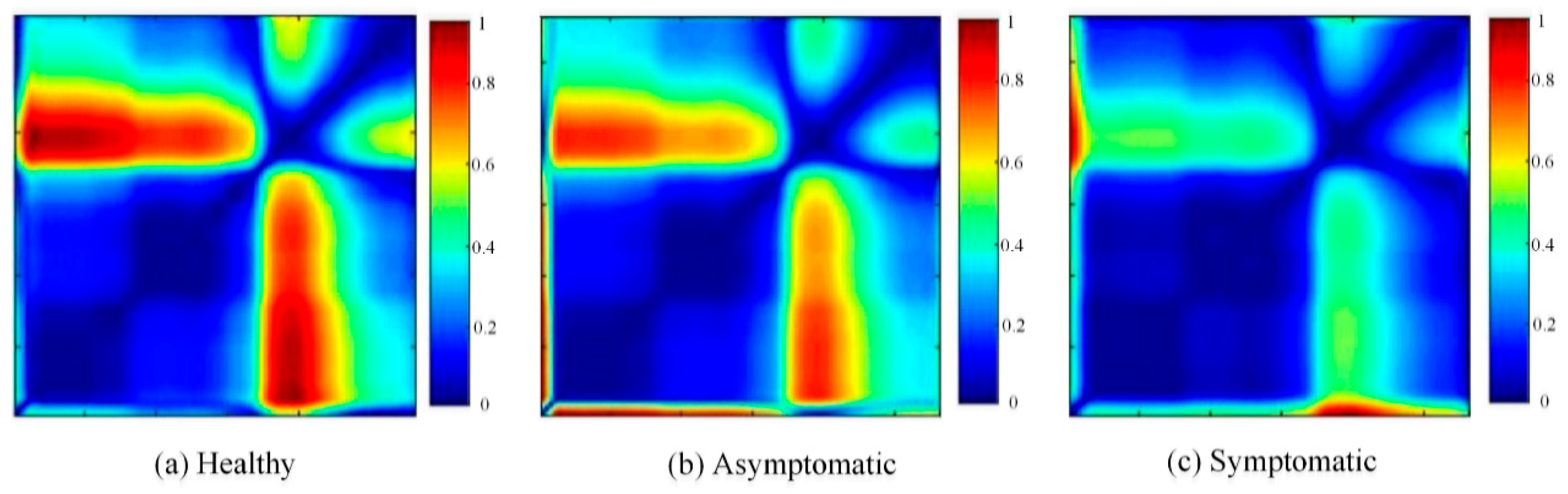
3.1. Different Infection States of Cotton Verticillium Wilt

The infection process of Verticillium wilt is divided into two stages: the asymptomatic stage and the symptomatic stage. Figure 4 shows cotton plants in different infection states. Healthy plants have no diseased leaves, grow normally, and show no signs of disease in the xylem of the stems. Cotton plants infected but asymptomatic have leaves that appear similar to those of healthy plants, with only slight yellowing at the edges and inside. The leaf morphology is normal, without curling. However, the xylem of the stems shows signs of disease. Already infected but in the incubation period, no obvious symptoms have been shown yet. At this stage, the hyphae of Verticillium dahliae produce spores and rapidly spread within the vascular tissue of the plant [37]. Cotton plants infected with symptomatic Verticillium wilt show significant differences compared to healthy plants. Yellow patches with irregular shapes appear between the edges of the leaves and the main veins. The color of the diseased spot gradually deepens, the edges of the diseased leaves curl up, and the vascular bundles in the stem turn brown. At this stage, Verticillium dahliae secretes toxins that degrade the cell walls of crop roots, heavily colonizing the plant’s xylem. The pathogen spreads towards the stem and leaves as water evaporates, eventually infecting the entire crop [38].

The development of cotton plants infected with Verticillium wilt over 1–15 days is shown in Figure 5. The horizontal axis represents the incubation period after inoculation, and the vertical axis represents the overall proportion of asymptomatic and symptomatic samples. It can be observed that symptomatic samples appear on the 9th day after inoculation. Days 9–12 mark the fastest progression of Verticillium wilt, during which most samples show symptoms. By the 14th day, all samples exhibit symptoms.

There is little difference between the spectral curves of healthy samples and asymptomatic samples, with healthy samples exhibiting higher spectral reflectance values. As the number of days post-infection increases, the spectral reflectance values of infected samples gradually decrease, as shown in Figure 6. The variation trend in the spectral curves of the three states of cotton plants is similar, and they all have a more obvious descending valley in the spectrum range of 1400–1500 nm, but the spectral curves of the healthy and asymptomatic plants have a greater decline of the reflectance in this range than that of the symptomatic plants. The spectral profile of cotton plants infected with asymptomatic Verticillium wilt shows little difference compared to that of healthy cotton plants. In symptomatic Verticillium wilt-infected cotton plants, the microscopic shrinkage of internal cells leads to macroscopic wilting of the cotton leaves, reduced plant water content, and a significant decrease in near-infrared spectral reflectance values.

There are noticeable texture differences in the 2D recurrence plots of spectral curves for different types of samples, as shown in Figure 7. The recurrence plot of healthy plants has a higher intensity of color mapping, while the intensity gradually decreases in the recurrence plot of asymptomatic infected plants. This reduction is associated with the lower reflectance of the spectral curves of asymptomatic plants compared to those of healthy plants. In symptomatic infected plants, the color mapping intensity of the recurrence plot decreases significantly, corresponding to a reflectance value of the spectral curve dropping below 0.4. In addition, we can observe that in the upper left corner and lower right corner of the diagonal in recurrence plots for cotton plants under different states, their internal shape and texture distribution are close. This may be due to the fact that their one-dimensional spectral curve changes tend to be similar.

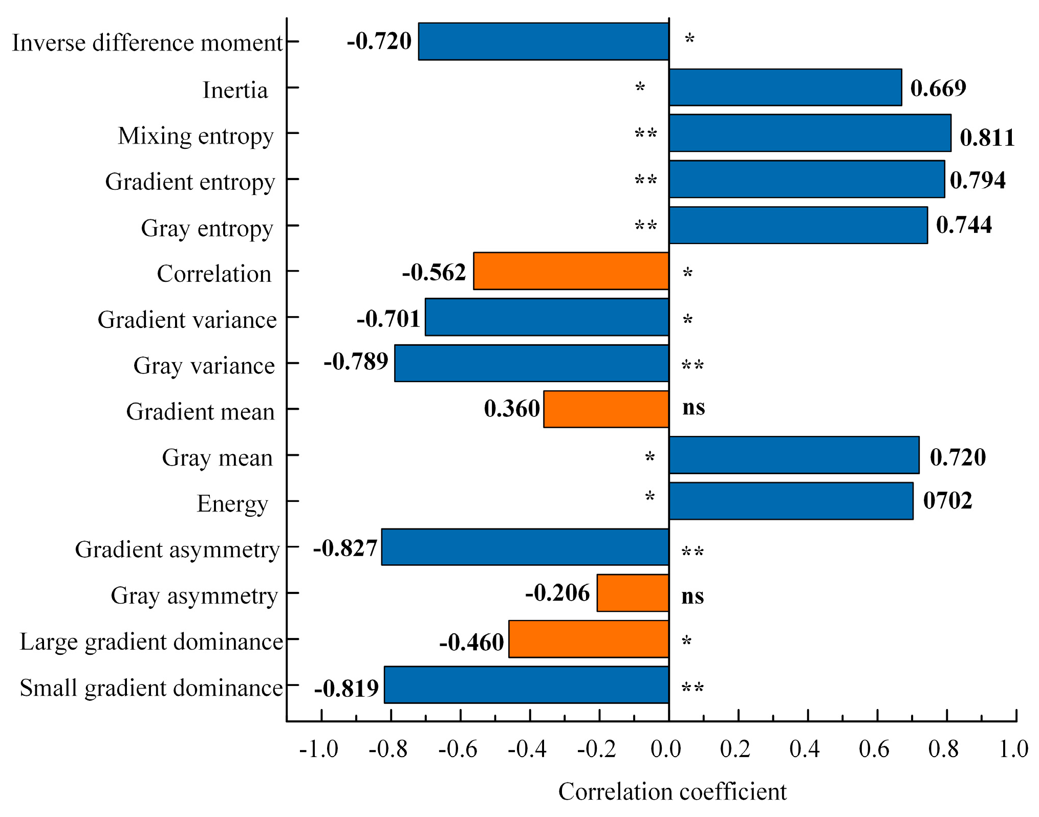
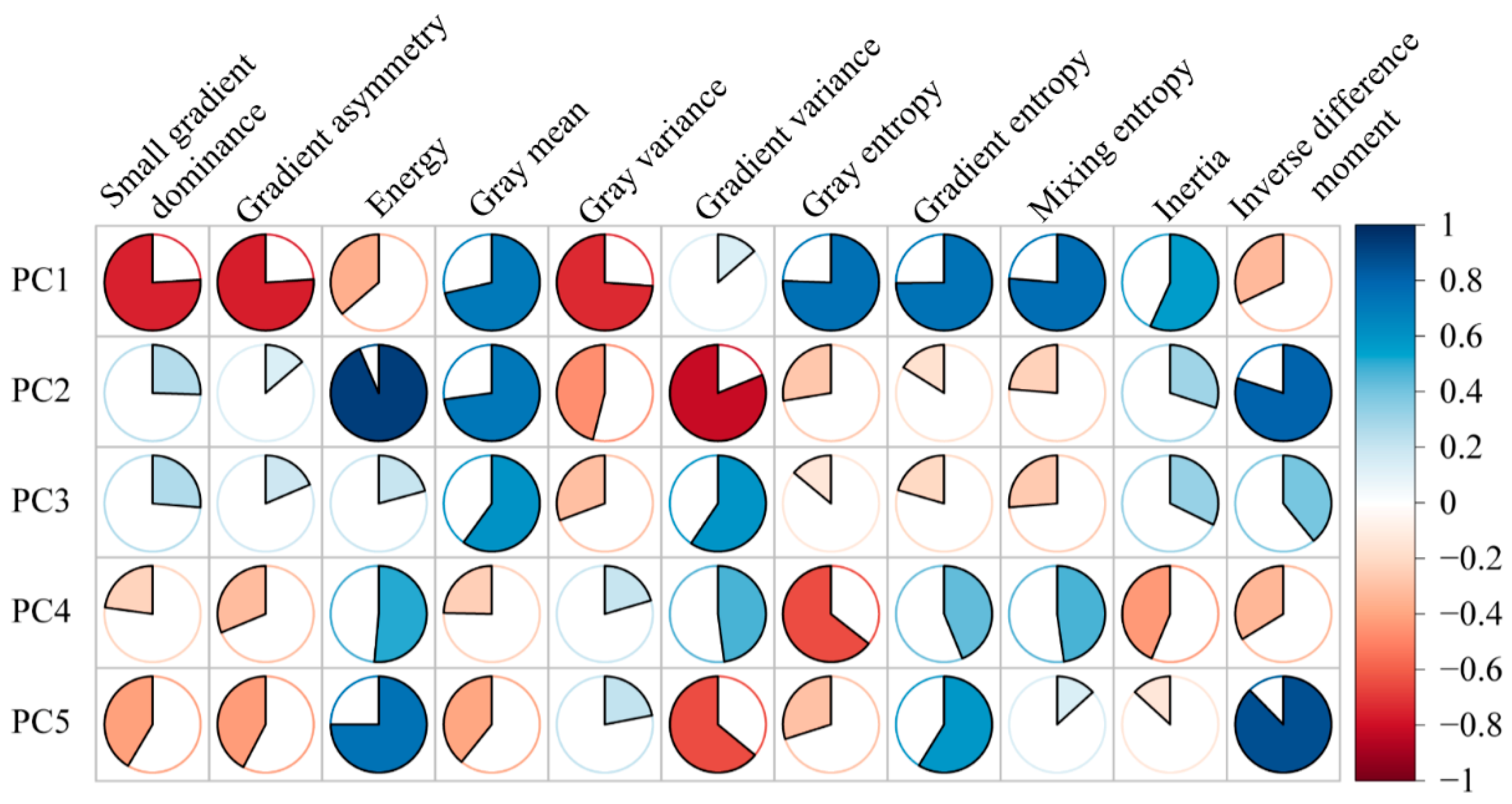
3.2. Correlation Between Texture Features

The original color recurrence images were converted to grayscale, and 15 texture features were extracted using the GLGCM method. The absolute values of the correlation coefficients for 11 texture features exceeded 0.6 (Figure 8), indicating a strong correlation with the class labels of healthy, asymptomatic, and symptomatic Verticillium wilt cotton plants. Among these features, five are related to entropy and asymmetry. For the remaining four texture features, two gradient-based texture features showed moderate correlation with the three class labels (0.4 < |r| < 0.6), while the other two features, namely gradient mean and gray asymmetry, had weak correlations with the class labels (0.2 < |r| < 0.4). In addition, 11 strongly correlated texture features showed very significant (p < 0.01) or significant (p < 0.05) correlation, and among the four moderately correlated and weakly correlated features, the correlation of gradient mean and gray asymmetry was not significant (p > 0.05), while the correlation of the other two features was significant. Consequently, combining significance and correlation, these four texture features (i.e., correlation, gradient mean, gray asymmetry, large gradient dominance) were removed to reduce the complexity and computational cost of the input features.

Based on the above results, a correlation analysis was conducted among the remaining 11 texture feature parameters. As shown in Figure 9, there is a strong correlation (0.6 < |r| < 0.8) among the three entropy features, which reflect the complexity of the image texture. Asymmetry features represent unevenness, while entropy features represent complexity. Due to the inherent unevenness and complexity of gray and gradient distributions, there is a very strong correlation (|r| > 0.8) between gradient asymmetry features and entropy features. Additionally, most texture parameters show varying degrees of correlation, indicating that principal component analysis should be applied to texture features to reduce significant information redundancy.

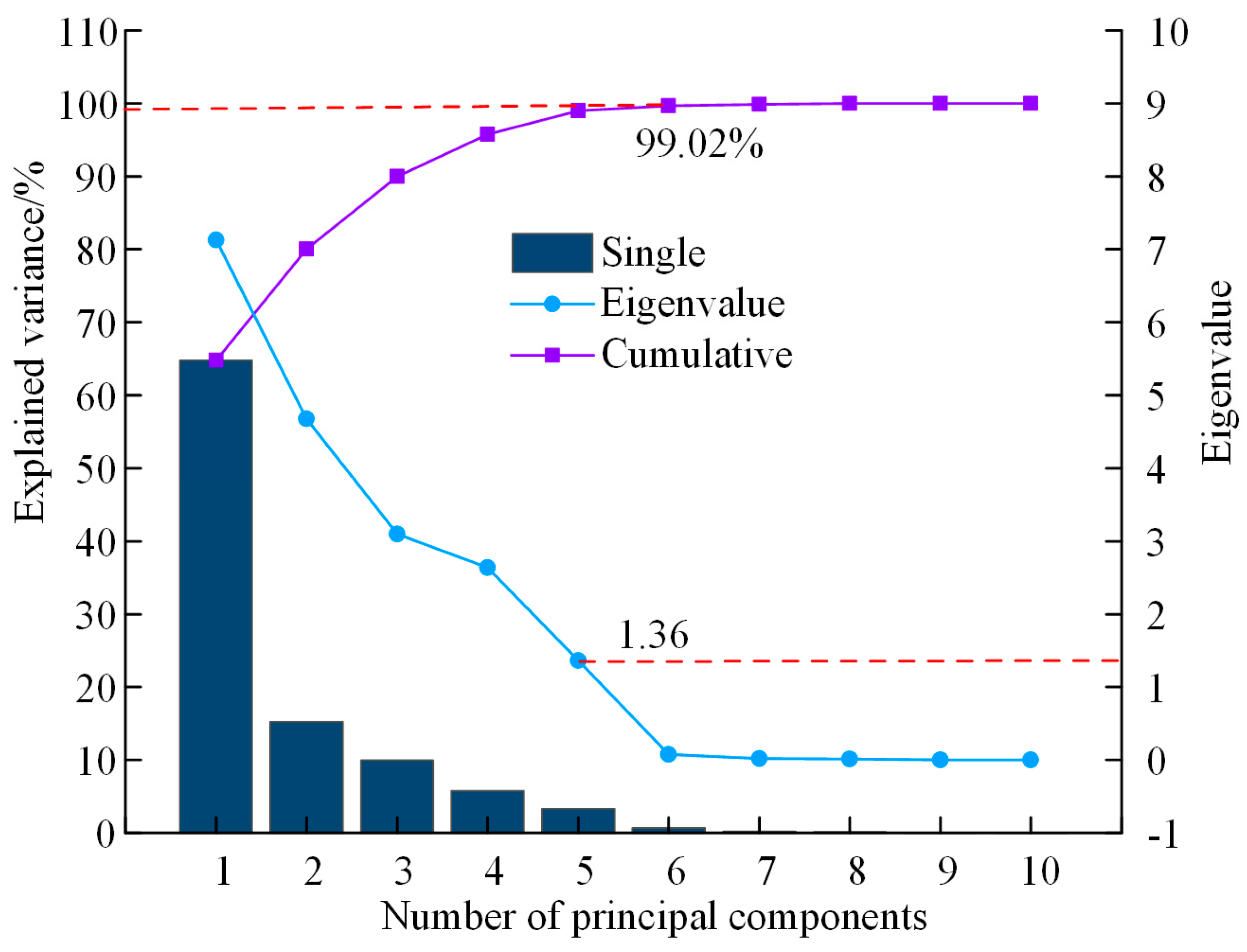
3.3. Determining the Principal Components That Describe the Texture Features

The core idea of PCA is to reduce the dimensionality of the data by converting multiple variables in the original dataset into a few unrelated principal components through linear transformations while preserving the most important information in the original data as much as possible. Principal component analysis was performed on the 11 texture feature parameters. The number of principal components extracted is determined according to whether the eigenvalue is greater than 1 and the cumulative contribution rate of variance is more than 90%. The first five principal components have eigenvalues greater than 1, and these five components account for a cumulative variance contribution rate of 99.02%, effectively explaining most of the information in the 11 texture feature parameters, as shown in Figure 10. Therefore, the first five principal components are determined to represent the texture feature parameter information of cotton Verticillium wilt spectral recurrence plots in different states.

From the loadings matrix plot in Figure 11, the area of the colored sectors reflects the magnitude of the absolute values of the loadings. The larger the area of the colored sector, the more information that principal component captures about the texture features. In the first principal component (PC1), the absolute values of the loadings for seven texture parameters exceed 0.70, primarily integrating information about small gradient dominance, gradient asymmetry, gray mean, gray variance, gray entropy, gradient entropy, and mixing entropy. The second principal component (PC2) mainly reflects the information of four features: energy, gray mean, gradient variance, and inverse difference moment, with the loading value for energy being greater than 0.90. The third principal component (PC3) mainly represents information about gray mean and gradient variance, with loadings of 0.60 and 0.59, respectively. The fourth principal component (PC4) primarily reflects gray entropy, with an absolute loading value of 0.64. The fifth principal component (PC5) mainly represents information about energy, gradient variance, gradient entropy, and inverse difference moment, with absolute loading values of 0.75, 0.64, 0.59, and 0.88, respectively.

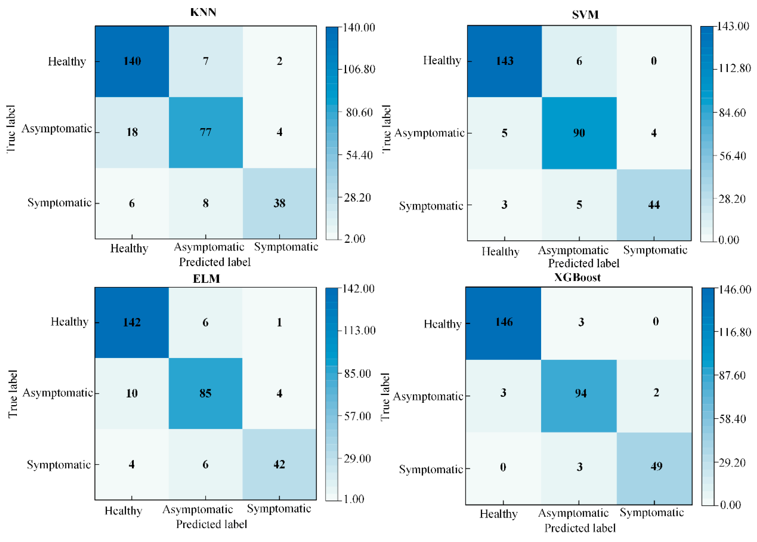
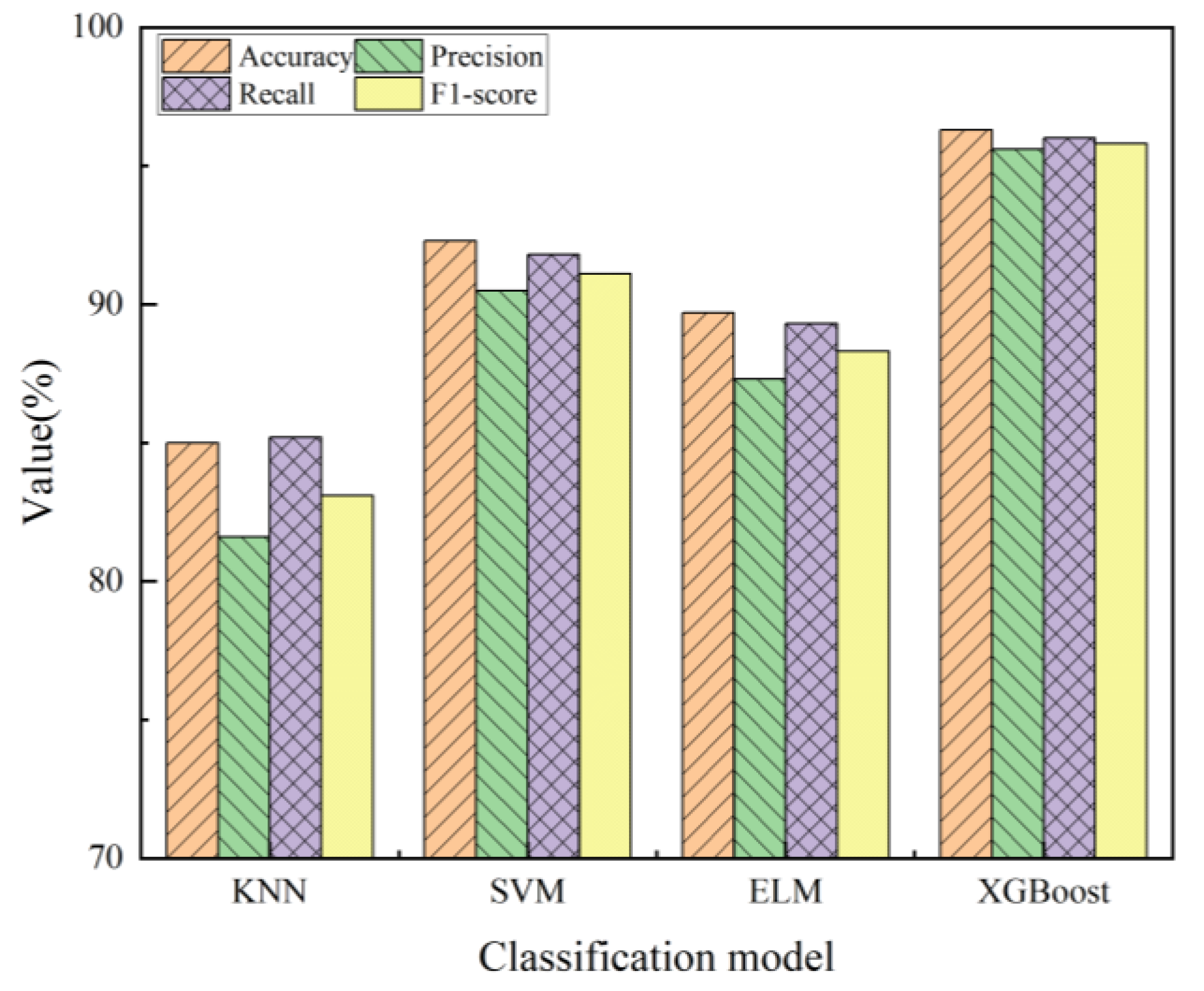
3.4. Comparison of Performance Between Different Classification Models

Classification models for detecting cotton Verticillium wilt in the “healthy–asymptomatic–symptomatic” three-class system were established using K-Nearest Neighbors (KNNs), support vector machine (SVM), Extreme Learning Machine (ELM), and eXtreme Gradient Boosting (XGBoost). The comparison of classification performance of Verticillium wilt in cotton using KNN, SVM, ELM, and XGBoost models is shown in

Table 2. Classification results of Verticillium wilt in cotton using KNN, SVM, ELM, and XGBoost models.

Model	Training Set				Test Set
	Accuracy	Precision	Recall	F1-Score	Accuracy	Precision	Recall	F1-Score
KNN	86.8%	83.5%	85.9%	84.7%	85.0%	81.6%	85.2%	83.1%
SVM	93.7%	91.2%	92.5%	91.9%	92.3%	90.5%	91.8%	91.1%
ELM	91.4%	88.7%	89.8%	89.3%	89.7%	87.3%	89.3%	88.3%
XGBoost	98.4%	96.3%	97.1%	96.7%	96.3%	95.6%	96.0%	95.8%

. For the training set and test set, the performance of the XGBoost model was the best, with the accuracy, precision, recall, and F₁-score being 98.4%, 96.3%, 97.1%, and 96.7%, respectively, followed by the SVM and ELM models; the KNN model was the worst. In addition, the four models have good classification performance on both the training set and the test set, and there is little difference between the model performance indicators of the training set and the test set, with strong generalization ability and no overfitting phenomenon. The confusion matrices for the test sets of the four models are shown in Figure 12. It can be observed that in KNN, ELM, and SVM models, more than 10 healthy samples and symptomatic samples were misclassified as asymptomatic samples. In the XGBoost model, 3 healthy samples were misclassified as asymptomatic, and 3 symptomatic samples were misclassified as asymptomatic. Comparatively, the XGBoost model had the fewest misclassifications, followed by the SVM and ELM models, while the KNN model had the most misclassifications.

Accuracy, precision, recall, and F1-score were used to further compare and analyze the performance of different machine learning classification models, as shown in Figure 13. Among the four machine learning classification models, the KNN model had the lowest overall classification performance. The ELM and SVM models showed improved classification performance compared to the KNN model, with increases in the corresponding classification metrics. The XGBoost model achieved the highest classification performance, with accuracy, precision, recall, and F1-score of 96.3%, 95.6%, 96%, and 95.8%, respectively. In summary, we realized the detection of early asymptomatic Verticillium wilt of cotton by converting hyperspectral curves into recurrence plots and extracting texture features for constructing machine learning models, and the classification accuracy of the XGBoost model for early asymptomatic Verticillium wilt reached 96.3%.

It is worth noting that Yang et al. [23] in their study reported an average accuracy of 90.62% for the detection of asymptomatic Verticillium wilt in cotton based on a logistic regression model with the wavelet features. Compared with our study, the classification accuracy is slightly lower. This may be due to the fact that the recurrence plot better highlights the subtle changes in the spectrum caused by V. dahliae infection and that the continuous wavelet transform is susceptible to the choice of wavelet basis function. Furthermore, differences between machine learning models cannot be ruled out. In summary, the resolution and differentiation of hyperspectral signals of cotton plants in different states were improved by the signal imaging of recurrence plots, which provided an important research method and strategy for the asymptomatic early detection of cotton Verticillium wilt.

4. Conclusions

This study demonstrated that extracting texture features after converting spectral curves into recurrence plots can be used for accurate detection of Verticillium wilt in the asymptomatic period. The ability to perform rapid, non-destructive detection of Verticillium wilt infection during the asymptomatic stage is crucial for preventing and controlling the large-scale spread of the disease. In this research, hyperspectral imaging and recurrence plots are combined with machine learning techniques for the early detection of cotton Verticillium wilt. The spectral curves of cotton in different states (healthy, asymptomatic, and symptomatic) were converted into recurrence plots, and fifteen texture features were extracted from the 2D recurrence plots using the GLGCM method. Through correlation analysis, a total of eleven highly correlated features were selected, and principal component analysis was further applied to reduce dimensionality, resulting in the first five principal components. These reduced dimensions were then input into KNN, SVM, ELM, and XGBoost classifiers. Among these models, the XGBoost model was proved to be more suitable for early asymptomatic detection of cotton Verticillium wilt compared to KNN, SVM, and ELM models. By applying the XGBoost model, accuracy, precision, recall, and F1-score reached 96.3%, 95.6%, 96%, and 95.8%, indicating high classification capability. Therefore, the proposed method is well-suited for the task of early detection of asymptomatic cotton Verticillium wilt.

This model can be used for rapid and convenient detection of asymptomatic cotton Verticillium wilt. Future research could focus on further validation in cotton fields, fully considering the diversity of cotton samples and the imbalance between diseased and healthy samples. Additionally, future studies could analyze and compare the effectiveness of other signal imaging methods (such as Gramian Angular Fields and Markov Transition Fields) for the early detection of asymptomatic Verticillium wilt in cotton. The integration of deep learning networks could further explore features within the images that are sensitive to Verticillium wilt information.

References

1. Bardak, A.; Çelik, S.; Erdoğan, O.; Ekinci, R.; Dumlupinar, Z. Association Mapping of Verticillium wilt disease in a worldwide collection of cotton (Gossypium hirsutum L.). Plants 2021, 10, 306. [Google Scholar] [CrossRef] [PubMed]
2. Tao, X.; Zhang, H.; Gao, M.; Li, M.; Zhao, T.; Guan, X. Pseudomonas species isolated via high-throughput screening significantly protect cotton plants against verticillium wilt. AMB Express 2020, 10, 193. [Google Scholar] [CrossRef] [PubMed]
3. Chen, J.Y.; Xiao, H.L.; Gui, Y.J.; Zhang, D.D.; Li, L.; Bao, Y.M.; Dai, X.F. Characterization of the Verticillium dahliae exoproteome involves in pathogenicity from cotton-containing medium. Front. Microbiol. 2016, 7, 1709. [Google Scholar] [CrossRef]
4. Calderón, R.; Navas-Cortés, J.A.; Zarco-Tejada, P.J. Early detection and quantification of Verticillium wilt in olive using hyperspectral and thermal imagery over large areas. Remote Sens. 2015, 7, 5584–5610. [Google Scholar] [CrossRef]
5. Yuan, Y.; Feng, H.; Wang, L.; Li, Z.; Shi, Y.; Zhao, L.; Feng, Z.; Zhu, H. Potential of endophytic fungi isolated from cotton roots for biological control against verticillium wilt disease. PLoS ONE 2017, 12, e0170557. [Google Scholar] [CrossRef]
6. Zahir, S.A.; Omar, A.F.; Jamlos, M.F.; Azmi, M.A.; Muncan, J. A review of visible and near-infrared (Vis-NIR) spectroscopy application in plant stress detection. Sens. Actuators A Phys. 2022, 338, 113468. [Google Scholar] [CrossRef]
7. Nguyen, C.; Sagan, V.; Maimaitiyiming, M.; Maimaitijiang, M.; Bhadra, S.; Kwasniewski, M.T. Early detection of plant viral disease using hyperspectral imaging and deep learning. Sensors 2021, 21, 742. [Google Scholar] [CrossRef]
8. Shin, M.Y.; Viejo, C.G.; Tongson, E.; Wiechel, T.; Taylor, P.W.; Fuentes, S. Early detection of Verticillium wilt of potatoes using near-infrared spectroscopy and machine learning modeling. Comput. Electron. Agric. 2023, 204, 107567. [Google Scholar] [CrossRef]
9. Jing, X.; Wang, J.; Song, X.; Xu, X.; Chen, B.; Huang, W. Continuous removal estimation method for the severity of cotton wilt disease. Trans. Chin. Soc. Agric. Eng. 2010, 26, 193–198. [Google Scholar] [CrossRef]
10. Chen, B.; Wang, G.; Liu, J.; Ma, Z.; Wang, J.; Li, T. Extraction of Photosynthetic Parameters from Hyperspectral Diseases of Cotton Leaves. Spectrosc. Spectr. Anal. 2018, 38, 1834–1838. [Google Scholar]
11. Zhang, N.; Zhang, X.; Shang, P.; Ma, R.; Yuan, X.; Li, L.; Bai, T. Detection of cotton verticillium wilt disease severity based on hyperspectrum and GWO-SVM. Remote Sens. 2023, 15, 3373. [Google Scholar] [CrossRef]
12. Lu, Z.; Huang, S.; Zhang, X.; Shi, Y.; Yang, W.; Zhu, L.; Huang, C. Intelligent identification on cotton verticillium wilt based on spectral and image feature fusion. Plant Methods 2023, 19, 75. [Google Scholar] [CrossRef] [PubMed]
13. Zarco-Tejada, P.J.; Camino, C.; Beck, P.S.; Calderon, R.; Hornero, A.; Hernández-Clemente, R.; Kattenborn, T.; Montes-Borrego, M.; Susca, L.; Morelli, M.; et al. Previsual symptoms of Xylella fastidiosa infection revealed in spectral plant-trait alterations. Nat. Plants 2018, 4, 432–439. [Google Scholar] [CrossRef]
14. Camino, C.; Calderón, R.; Parnell, S.; Dierkes, H.; Chemin, Y.; Román-Écija, M.; Montes-Borrego, M.; Landa, B.B.; Navas-Cortes, J.A.; Zarco-Tejada, P.J.; et al. Detection of Xylella fastidiosa in almond orchards by synergic use of an epidemic spread model and remotely sensed plant traits. Remote Sens. Environ. 2021, 260, 112420. [Google Scholar] [CrossRef]
15. Dutta, A.; Tyagi, R.; Chattopadhyay, A.; Chatterjee, D.; Sarkar, A.; Lall, B.; Sharma, S. Early detection of wilt in Cajanus cajan using satellite hyperspectral images: Development and validation of disease-specific spectral index with integrated methodology. Comput. Electron. Agric. 2024, 219, 108784. [Google Scholar] [CrossRef]
16. Riefolo, C.; Antelmi, I.; Castrignanò, A.; Ruggieri, S.; Galeone, C.; Belmonte, A.; Muolo, M.R.; Ranieri, N.A.; Labarile, R.; Gadaleta, G.; et al. Assessment of the hyperspectral data analysis as a tool to diagnose Xylella fastidiosa in the asymptomatic leaves of olive plants. Plants 2021, 10, 683. [Google Scholar] [CrossRef]
17. Cao, Y.; Yuan, P.; Xu, H.; Martínez-Ortega, J.F.; Feng, J.; Zhai, Z. Detecting asymptomatic infections of rice bacterial leaf blight using hyperspectral imaging and 3-dimensional convolutional neural network with spectral dilated convolution. Front. Plant Sci. 2022, 13, 963170. [Google Scholar] [CrossRef]
18. Li, W.; Guo, Y.; Yang, W.; Huang, L.; Zhang, J.; Peng, J.; Lan, Y. Severity Assessment of Cotton Canopy Verticillium Wilt by Machine Learning Based on Feature Selection and Optimization Algorithm Using UAV Hyperspectral Data. Remote Sens. 2024, 16, 4637. [Google Scholar] [CrossRef]
19. He, Q.; McLellan, H.; Boevink, P.C.; Birch, P.R. All roads lead to susceptibility: The many modes of action of fungal and oomycete intracellular effectors. Plant Commun. 2020, 1, 12. [Google Scholar] [CrossRef]
20. Kubicek, C.P.; Starr, T.L.; Glass, N.L. Plant cell wall–degrading enzymes and their secretion in plant-pathogenic fungi. Annu. Rev. Phytopathol. 2014, 52, 427–451. [Google Scholar] [CrossRef]
21. Trapero, C.; Alcántara, E.; Jiménez, J.; Amaro-Ventura, M.C.; Romero, J.; Koopmann, B.; Karlovsky, P.; Von Tiedemann, A.; Pérez-Rodríguez, M.; López-Escudero, F.J. Starch hydrolysis and vessel occlusion related to wilt symptoms in olive stems of susceptible cultivars infected by Verticillium dahliae. Front. Plant Sci. 2018, 9, 72. [Google Scholar] [CrossRef]
22. Gao, Z.; Khot, L.R.; Naidu, R.A.; Zhang, Q. Early detection of grapevine leafroll disease in a red-berried wine grape cultivar using hyperspectral imaging. Comput. Electron. Agric. 2020, 179, 105807. [Google Scholar] [CrossRef]
23. Yang, M.; Kang, X.; Qiu, X.; Ma, L.; Ren, H.; Huang, C.; Zhang, Z.; Lv, X. Method for early diagnosis of verticillium wilt in cotton based on chlorophyll fluorescence and hyperspectral technology. Comput. Electron. Agric. 2024, 216, 108497. [Google Scholar] [CrossRef]
24. Pitsik, E.; Frolov, N.; Hauke Kraemer, K.; Grubov, V.; Maksimenko, V.; Kurths, J.; Hramov, A. Motor execution reduces EEG signals complexity: Recurrence quantification analysis study. Chaos Interdiscip. J. Nonlinear Sci. 2020, 30, 023111. [Google Scholar] [CrossRef]
25. Seo, D.; Nam, H. Deep rp-cnn for burst signal detection in cognitive radios. IEEE Access 2020, 8, 167164–167171. [Google Scholar] [CrossRef]
26. Mathunjwa, B.M.; Lin, Y.T.; Lin, C.H.; Abbod, M.F.; Shieh, J.S. ECG arrhythmia classification by using a recurrence plot and convolutional neural network. Biomed. Signal Process. Control 2021, 64, 102262. [Google Scholar] [CrossRef]
27. Masalegoo, S.E.; Soleimani, A.; Saeedi Masine, H. Experimental fault detection of rotating machinery through chaos-based tools of recurrence plot and recurrence quantitative analysis. Arch. Appl. Mech. 2023, 93, 1259–1272. [Google Scholar] [CrossRef]
28. Zhang, Y.; Zheng, M.; Zhu, R.; Ma, R. Adulteration discrimination and analysis of fresh and frozen-thawed minced adulterated mutton using hyperspectral images combined with recurrence plot and convolutional neural network. Meat Sci. 2022, 192, 108900. [Google Scholar] [CrossRef]
29. Yang, Y.; Peng, J.; Fan, P. A non-destructive dropped fruit impact signal imaging-based deep learning approach for smart sorting of kiwifruit. Comput. Electron. Agric. 2022, 202, 107380. [Google Scholar] [CrossRef]
30. GB/T 22101.5-2009; Technical Specifications for Evaluation of Cotton Resistance to Diseases and Pests—Part 5: Verticillium Wilt. General Administration of Quality Supervision, Inspection and Quarantine of the People’s Republic of China. Standardization Administration of China: Beijing, China, 2009.
31. Eckmann, J.P.; Kamphorst, S.O.; Ruelle, D. Recurrence plots of dynamical systems. World Sci. Ser. Nonlinear Sci. Ser. A 1995, 16, 441–446. [Google Scholar] [CrossRef]
32. Rogers, M.; Blanc-Talon, J.; Urschler, M.; Delmas, P. Wavelength and texture feature selection for hyperspectral imaging: A systematic literature review. J. Food Meas. Charact. 2023, 17, 6039–6064. [Google Scholar] [CrossRef]
33. Guru, D.S.; Sharath, Y.H.; Manjunath, S. Texture features and KNN in classification of flower images. IJCA 2010, 37, 21–29. [Google Scholar] [CrossRef]
34. Manavalan, R. Towards an intelligent approaches for cotton diseases detection: A review. Comput. Electron. Agric. 2022, 200, 107255. [Google Scholar] [CrossRef]
35. Chorowski, J.; Wang, J.; Zurada, J.M. Review and performance comparison of SVM-and ELM-based classifiers. Neurocomputing 2014, 128, 507–516. [Google Scholar] [CrossRef]
36. Munera, S.; Gómez-Sanchís, J.; Aleixos, N.; Vila-Francés, J.; Colelli, G.; Cubero, S.; Soler, E.; Blasco, J. Discrimination of common defects in loquat fruit cv. ‘Algerie’ using hyperspectral imaging and machine learning techniques. Postharvest Biol. Technol. 2021, 171, 111356. [Google Scholar] [CrossRef]
37. Tian, J.; Kong, Z. Live-cell imaging elaborating epidermal invasion and vascular proliferation/colonization strategy of Verticillium dahliae in host plants. Mol. Plant Pathol. 2022, 23, 895–900. [Google Scholar] [CrossRef] [PubMed]
38. Tang, W.; Wu, N.; Xiao, Q.; Chen, S.; Gao, P.; He, Y.; Feng, L. Early detection of cotton verticillium wilt based on root magnetic resonance images. Front. Plant Sci. 2023, 14, 1135718. [Google Scholar] [CrossRef]
Figure 1. Experimental process.
Agronomy 15 00213 g001
Figure 2. Hyperspectral imaging system.
Agronomy 15 00213 g002
Figure 3. Raw mean spectral curves of all cotton plants in different states.
Agronomy 15 00213 g003
Figure 4. Cotton plants in different states. (a) healthy; (b) asymptomatic; and (c) symptomatic. The red arrows in the figure show the vascular tissues of cotton plants in different states.
Agronomy 15 00213 g004
Figure 5. The incidence of Verticillium wilt in plants within 1–15 days after inoculation.
Agronomy 15 00213 g005
Figure 6. Typical spectral curves of the three types of samples.
Agronomy 15 00213 g006
Figure 7. Two-dimensional recurrence plots of the average spectral curves for the three types of samples. The color bar values 0–1 indicate the range of recurrence values.
Agronomy 15 00213 g007
Figure 8. Results of the correlation analysis between texture features and the three class labels. ** represents p < 0.01; * represents p < 0.05; and ns represents p > 0.05.
Agronomy 15 00213 g008
Figure 9. Mutual correlation coefficients among the 11 texture features.
Agronomy 15 00213 g009
Figure 10. Eigenvalues and variance contribution rates of each principal component.
Agronomy 15 00213 g010
Figure 11. Loadings matrix of the first five principal components extracted from the principal component analysis.
Agronomy 15 00213 g011
Figure 12. Confusion matrices of different classification models.
Agronomy 15 00213 g012
Figure 13. Performance comparison of KNN, SVM, ELM, and XGBoost models for Verticillium wilt detection.
Agronomy 15 00213 g013