Hybrid Plant Growth: Integrating Stochastic, Empirical, and Optimization Models with Machine Learning for Controlled Environment Agriculture

Abstract

Controlled Environment Agriculture (CEA) offers a viable solution for sustainable crop production, yet the optimization of the latter requires precise modeling and resource management. This study introduces a novel hybrid plant growth model integrating stochastic, empirical, and optimization approaches, using Internet of Things sensors for real-time data collection. Unlike traditional methods, the hybrid model systematically captures environmental variability, simulates plant growth dynamics, and optimizes resource inputs. The prototype growth chamber, equipped with IoT sensors for monitoring environmental parameters such as light intensity, temperature, CO₂, humidity, and water intake, was primarily used to provide accurate input data for the model and specifically light intensity, water intake and nutrient intake. While experimental tests on lettuce were conducted to validate initial environmental conditions, this study was focused on simulation-based analysis. Specific tests simulated plant responses to varying levels of light, water, and nutrients, enabling the validation of the proposed hybrid model. We varied light durations between 6 and 14 h/day, watering levels between 5 and 10 L/day, and nutrient concentrations between 3 and 11 g/day. Additional simulations modeled different sowing intervals to capture internal plant variability. The results demonstrated that the optimal growth conditions were 14 h/day of light, 9 L/day of water, and 5 g/day of nutrients; maximized plant biomass (200 g), leaf area (800 cm²), and height (90 cm). Key novel metrics developed in this study, the Growth Efficiency Ratio (GER) and Plant Growth Index (PGI), provided solid tools for evaluating plant performance and resource efficiency. Simulations showed that GER peaked at 0.6 for approximately 200 units of combined inputs, beyond which diminishing returns were observed. PGI increased to 0.8 to day 20 and saturated to 1 by day 30. The role of IoT sensors was critical in enhancing model accuracy and replicability by supplying real-time data on environmental variability. The hybrid model’s adaptability in the future may offer scalability to diverse crop types and environmental settings, establishing a foundation for its integration into decision-support systems for large-scale indoor farming.

1. Introduction

The increasing global demand for sustainable food production has driven the development of innovative solutions in agriculture. Controlled Environment Agriculture (CEA) represents a promising approach to address this challenge by enabling precise control over environmental factors, such as light, temperature, humidity, water, and nutrients, to optimize crop growth while minimizing resource wastage [1,2]. Despite its potential, achieving a balance between resource inputs and maximizing crop yields remains a critical challenge, particularly in resource-limited settings. To address this, researchers have focused on developing models and technologies that predict, simulate, and optimize plant growth under various environmental conditions [3,4].

Previous studies in the field of CEA have explored various modeling approaches. Empirical models, such as linear and nonlinear regression, have been widely used to capture relationships between environmental inputs and plant growth outputs. However, these models are often limited by their reliance on specific datasets and lack the flexibility to incorporate variability [4,5,6]. Stochastic models, introduced to account for environmental uncertainties, provide a framework for simulating random fluctuations in growth conditions, such as light or temperature variability. Despite their strengths, these models frequently lack integration with real-time data sources, limiting their practical applicability [6,7]. Optimization techniques, including genetic algorithms and linear programming, have been employed to enhance resource usage in CEA systems but are often applied in isolation rather than as part of an integrated framework [8,9,10].

Recent advances in metrics and tools for plant growth evaluation include innovations like StoManager, which measures over 30 stomatal and guard cell metrics to study leaf physiology [11]. While such metrics offer detailed insights, they primarily focus on specific parameters rather than providing a comprehensive framework for growth and resource optimization. Similarly, imaging-based approaches allow for precise non-destructive measurements of plant traits but lack the multidimensional perspective needed for integrated decision-making.

Machine learning has shown promise for predicting plant growth and optimizing resource allocation by processing large datasets and uncovering complex patterns in plant-environment interactions. However, many machine learning-based studies lack physiological insights and fail to integrate stochastic and empirical models, limiting their robustness and interpretability. Additionally, IoT technologies have gained prominence in CEA by enabling real-time monitoring of environmental variables, such as temperature, humidity, CO₂ concentration, and light intensity [12]. While IoT enhances data accuracy and replicability, its integration into hybrid modeling frameworks remains underexplored.

Despite these advancements, existing tools and models fall short in offering a unified approach that combines the strengths of stochastic, empirical, and optimization methods with real-time IoT data. Furthermore, the absence of comprehensive metrics to evaluate both plant growth and resource efficiency, as well as their adaptability across diverse crops, leaves a significant gap in the literature.

To address these gaps, this study proposes a novel hybrid plant growth model with machine learning to enhance predictive accuracy and robustness. By incorporating IoT sensors for real-time data collection, the model dynamically adapts to varying environmental conditions, improving both accuracy and replicability. The contributions of this study include:

1.

Development of a Hybrid Plant Growth Model:

An integrated framework combining stochastic, empirical, and optimization approaches to simulate and optimize lettuce growth in controlled environments.

2.

Introduction of Innovative Metrics:

Development of the Growth Efficiency Ratio (GER) and Plant Growth Index (PGI), providing comprehensive evaluation of resource efficiency and plant health.

3.

Machine Learning for Metric Optimization:

Application of linear regression to empirically derive weights for the PGI metric.

4.

Cooling System Efficiency Analysis:

Assessment of cooling performance using the Coefficient of Performance (COP) to optimize energy use in the prototype growth chamber.

5.

Comprehensive Simulation:

Simulations conducted under varying environmental scenarios.

6.

Transferability of Models and Metrics:

Design of adaptable hybrid models and metrics for application to other crops and controlled agriculture systems.

Through a case study on indoor lettuce growth, this research demonstrates the hybrid model’s ability to optimize resource usage, maximize crop yields, and improve decision-making in CEA systems. Lettuce was selected for its widespread cultivation in controlled environments, rapid growth cycle, and sensitivity to environmental conditions, making it an ideal model crop for evaluating and refining growth models and metrics. By bridging the gap between theoretical modeling and practical application, this study contributes to advancing smart agriculture technologies and decision-support tools for long-term sustainability. The findings of this study suggest potential integration into Decision Support Systems (DSS) for enhanced agricultural management. The GER and PGI metrics provide actionable insights that could inform resource allocation strategies in real time. By embedding the hybrid model into DSS platforms, growers could access recommendations on optimal water, nutrient, and light levels tailored to their specific setups. This integration could facilitate real-time monitoring and decision-making in CEA systems, particularly in large-scale operations where efficient resource use is critical.

2. Materials and Methods

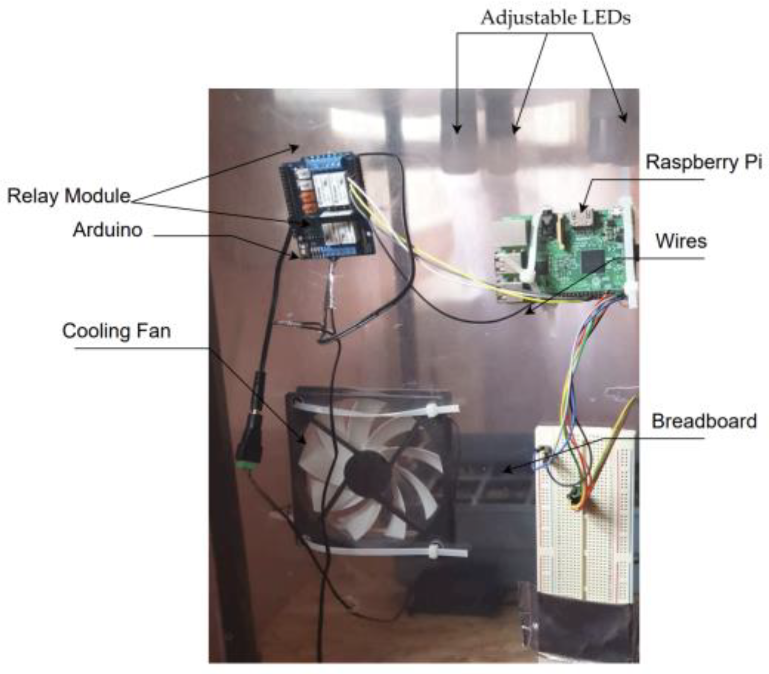
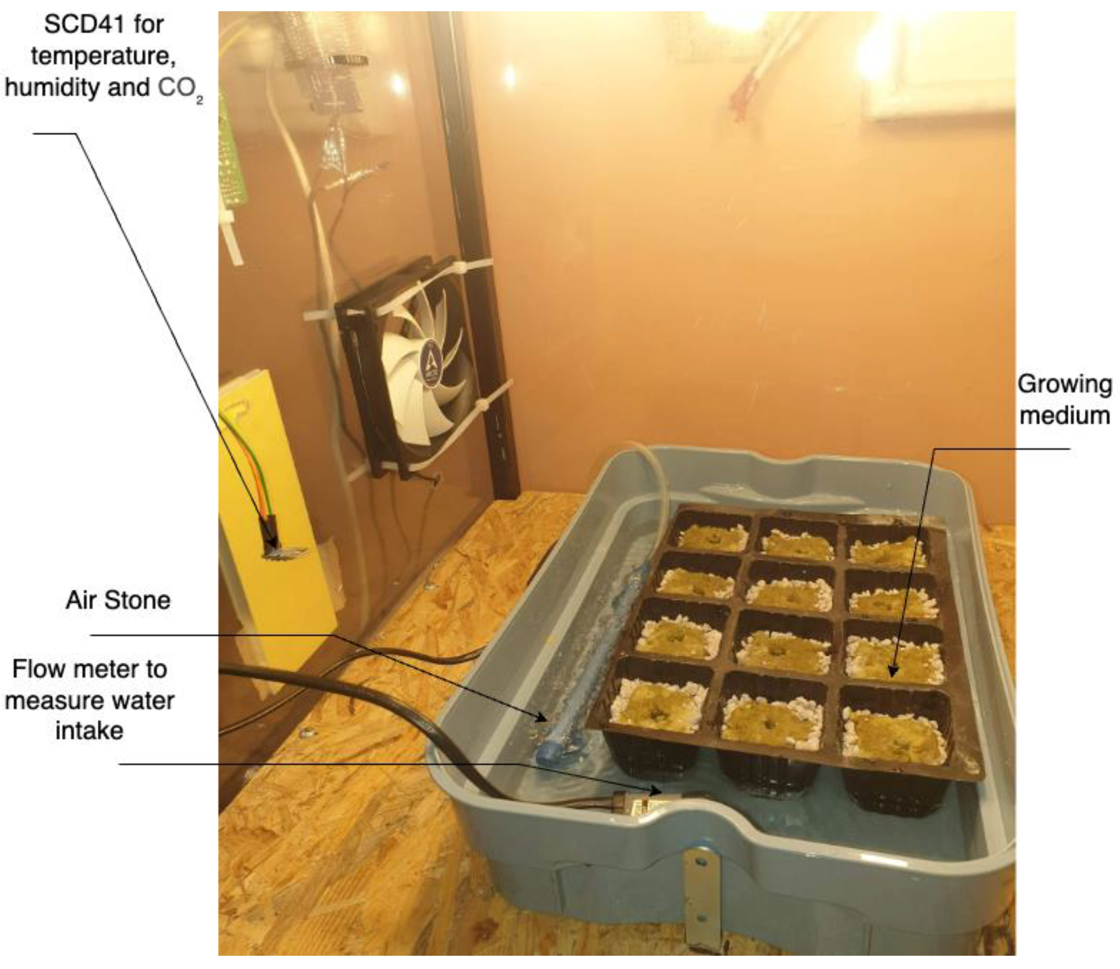
In this study, a combination of experimental prototype development in Figure 1 and Figure 2 and simulation modeling using python shown in Appendixes A.1 and A.2 was utilized to study the growth and development of lettuce under controlled environment conditions. A prototype growth chamber was constructed to test key parameters, providing a basis for the simulated datasets and model validation. The chamber was designed to replicate optimal growing conditions, including temperature regulation via a cooling system, adjustable light intensity, and automated irrigation systems.

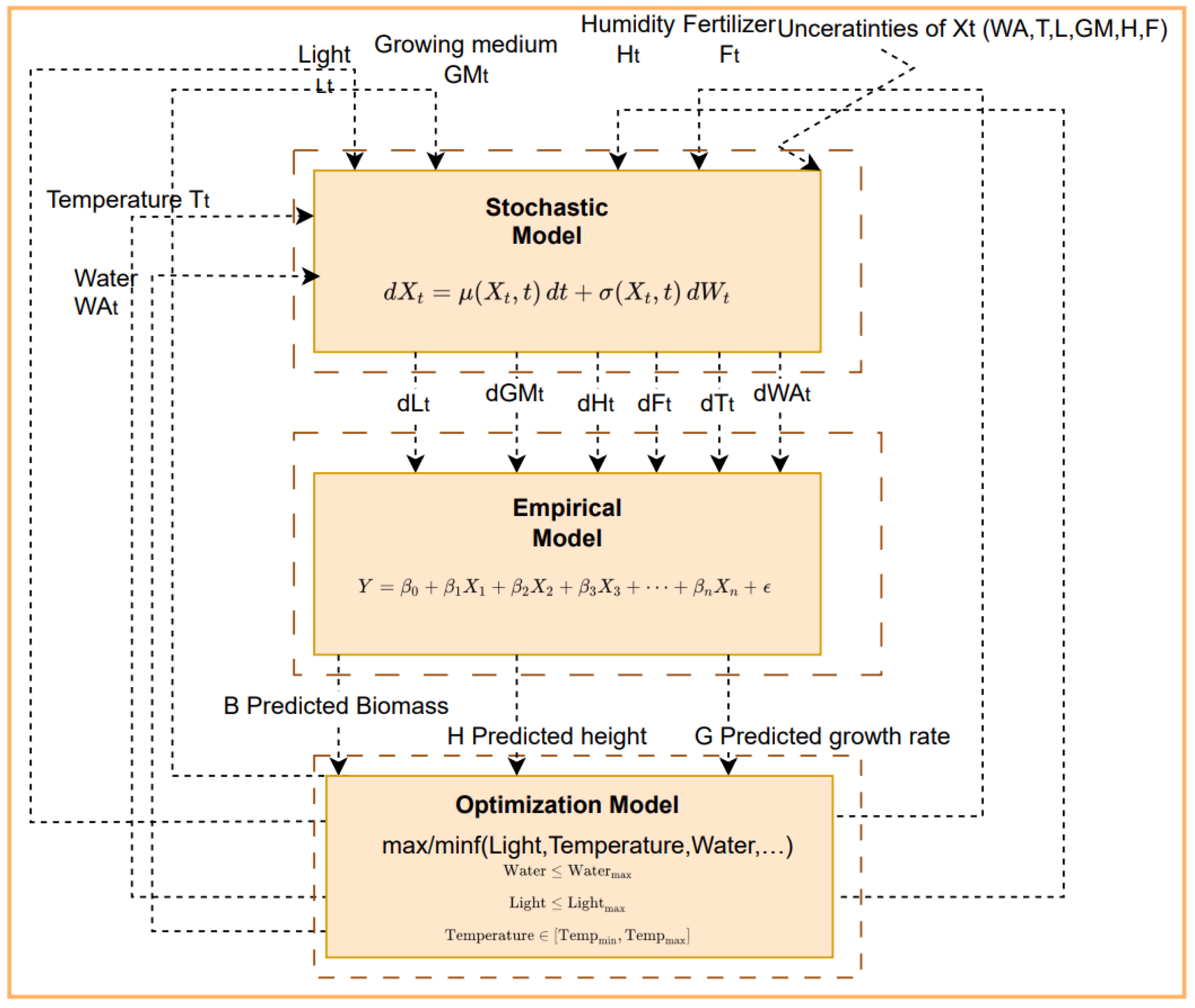
Our hybrid model combines stochastic, empirical, and optimization approaches, the relationship between these three models forms a conceptual, interconnected framework where each model informs and supplements the next one.

2.1. Data Collection

The prototype growing chamber in Figure 1 and Figure 2 is a controlled environment system designed to optimize and monitor plant growth conditions. It features a transparent enclosure from plexiglass to allow visual inspection while maintaining a sealed environment. A cooling fan is installed to ensure proper air circulation, preventing stagnation and regulating temperature and humidity. The system includes adjustable LED grow lights mounted inside the chamber, which provide a customizable light spectrum and intensity to simulate daylight cycles for photosynthesis, enabling precise control of light conditions to suit the needs of different growth stages.

A Raspberry Pi serves as the central processing unit for our IoT data collection and control, while a relay module connected to an Arduino manages devices such as the fan, and LED lights. A breadboard facilitates prototyping and the integration of the combined sensor for temperature, humidity, and CO₂. This IoT-enabled setup supports real-time data collection and environmental regulation, making it ideal for precision agriculture and smart farming technologies.

Fan: A cooling fan used for air circulation and temperature control inside the prototype.

Raspberry Pi: The green circuit board on the right side is a Raspberry Pi, a single-board computer used for controlling the system, processing data, and connecting sensors to the Raspberry Pi through the breadboard.

Relay Module: The blue board on the upper left is a relay module, used to control high-power devices, in our case for the fan with low-power signals from the Raspberry Pi.

Arduino: The board connected to the relay module is used for interfacing with sensors.

Breadboard: The white perforated board below the Raspberry Pi is a breadboard, used for building and testing electronic circuits without soldering.

Wires: Various wires connect the components, allowing for power and data transmission.

Transparent Enclosure: The clear enclosure made of plexiglass provides a sealed environment for the system.

Integrated Sensor SCD41: The integrated sensor that monitors temperature, humidity, and CO₂ levels in real-time.

Air Stone: Facilitates oxygenation by diffusing air into the water, increasing dissolved oxygen levels and supporting healthy root development.

Flow Meter: Measures the precise amount of water delivered to plants.

Growing Medium: The rockwool that holds the plants in place and provides structural support, enabling efficient nutrient and water absorption for healthy growth.

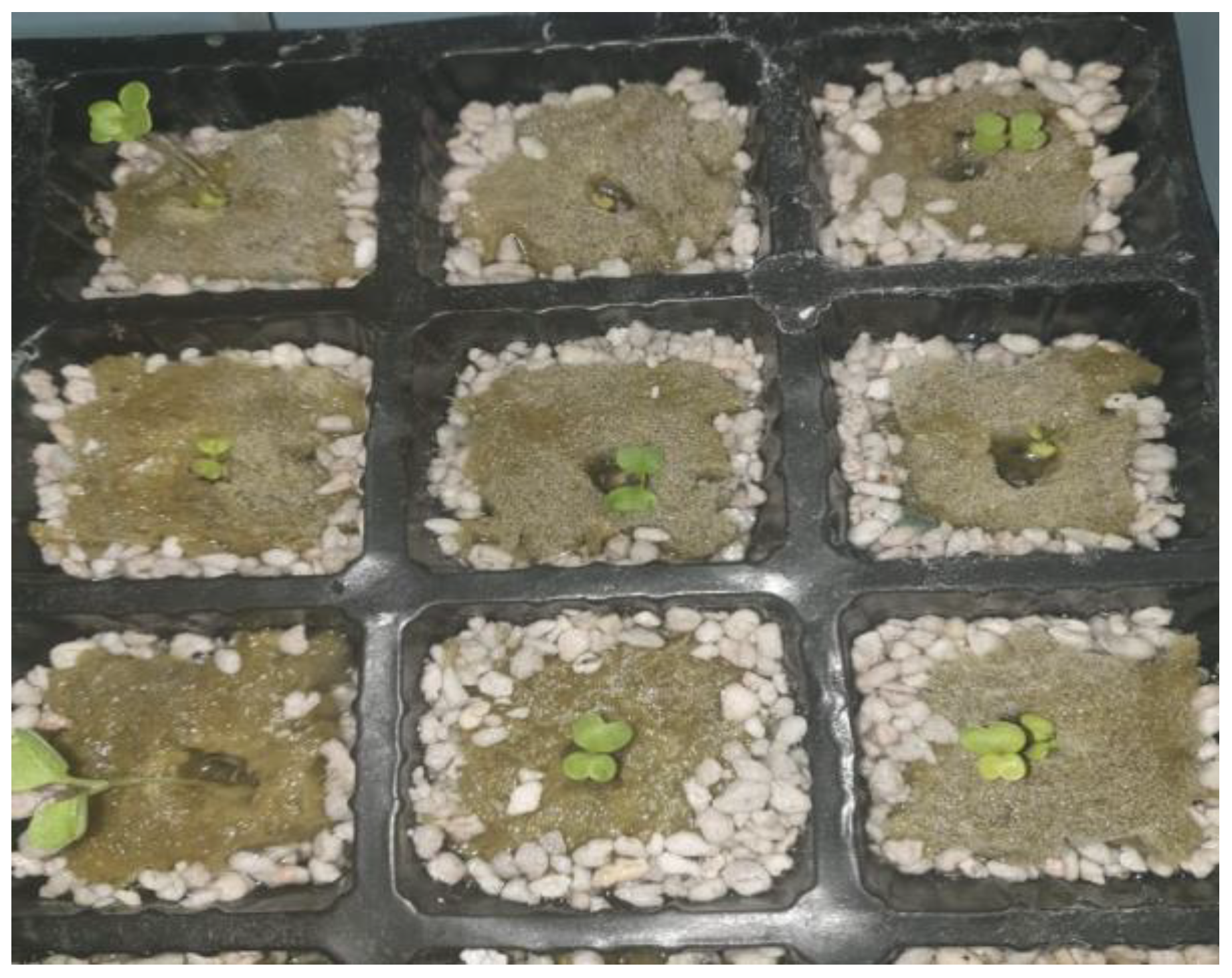
Initial data on environmental inputs, including light intensity, water intake, nutrient levels were collected directly from the prototype using IoT sensors and image analysis. To validate early growth stages in Figure 3, lettuce seedlings were monitored inside the controlled chamber.

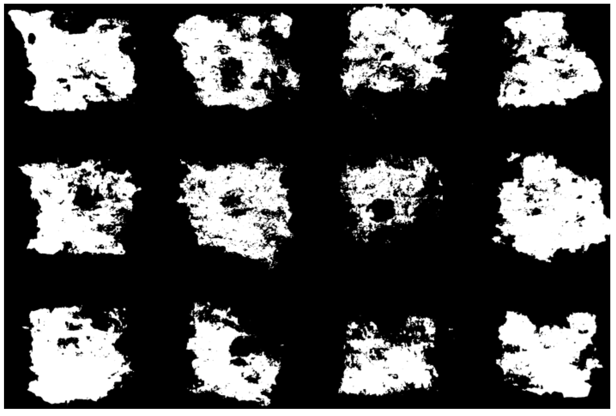
Figure 4 highlights the uniform arrangement of seedlings in the growing medium and the precise environmental conditions maintained during the study. Image analysis was subsequently employed to calculate water and nutrient intake. The threshold segmentation technique, as shown in Figure 5, was processed using PlantCV software with version 3.13.0 to distinguish wet and dry areas in the growing medium. Wet pixels were counted and converted into physical area (cm²) through calibration, allowing precise quantification of water absorption based on the medium’s water-holding capacity. Nutrient uptake was then calculated by multiplying the absorbed water volume with the nutrient concentration in the irrigation solution. This method builds upon the approach discussed in our previous work on monitoring plant growth through phenotyping and image analysis, where similar techniques were employed to study photosynthesis efficiency and resource utilization [13].

2.2. Hybrid Model: Plant Growth and Resource Efficiency

The hybrid model integrates stochastic, empirical, and optimization approaches to provide a comprehensive framework for plant growth prediction and resource optimization. Each component contributes a distinct perspective, capturing variability, quantifying relationships, and identifying optimal conditions.

2.2.1. Model and Its Components

Stochastic Model Equation

The first choice is environmental variability in our simulations, as it utilizes the stochastic differential equation (SDE) to model the growth factors including as light, water, and temperature. This approach captures both the deterministic trends in environmental conditions and the inherent random fluctuations.

The general form in Equation (1) for each environmental factor X(t) (such as light, water, or temperature) [14] of the stochastic equation is:

$$\mathrm{d}{X}_t=\mu (X_t,t) \mathrm{dt}+\sigma (X_t,t) d{W}_t$$

(1)

where μ($X_t,t$) represents the drift term modeling the deterministic trend, σ($X_t,t$) denotes the diffusion term accounting for random fluctuations, and $d{W}_t$ corresponds to the Brownian motion. This equation provides a robust framework for simulating dynamic and uncertain environmental conditions.

In this case study as shown in Figure 6, we adapted the general form of the stochastic differential equation to model key environmental inputs—light, water, and temperature—by tailoring the deterministic component (μ) and random variability (σ) to reflect their specific dynamics. For light, μ represented the planned exposure schedule, while σaccounted for fluctuations such as lighting failures. For water, μ corresponded to scheduled irrigation levels, and σ captured inconsistencies in absorption rates. Similarly, for temperature, μ indicated expected trends from cooling or heating systems, and σ modeled unexpected changes such as equipment malfunctions.

By solving the SDEs, we simulated multiple scenarios of environmental conditions under both expected and random influences [15]. Each simulation run produced a different outcome based on the random components, allowing us to generate stochastic predictions for future environmental conditions [16].

Empirical Modeling for Plant Growth Dynamics

The second step is the empirical model that starts by using datasets that were recorded on plant growth metrics under various controlled environmental conditions in the previous step. These data points allow the estimation of coefficients $b_1,b_2,b_3\dots b_n$ for each factor, providing a functional form of the relationship between inputs and outputs. This served as the basis for calculating biomass and height which was validated against simulation results.

The empirical model represented by Equation (2) is a common mathematical model [17]. The model was employed to calculate key plant growth metrics such as biomass yield, plant height, and growth rate:

$$\mathrm{Y}=b_0+b_1{X}_1+b_2{X}_2+b_3{X}_3+\cdots +b_n{X}_n+e$$

(2)

where Y is the target growth metric such as biomass yield or plant height; $X_1,X_2,X_3 \dots X_n$ are input factors like light intensity, water intake, nutrient levels, and temperature; $b_0$ is the intercept representing the baseline value of Y when all inputs are zero; $b_1,b_2,b_3 \dots b_n$ are coefficients indicating the contribution of each factor to Y; and e is the error term accounting for unexplained variability.

Optimization Modeling for Resource Efficiency

We determined, using various simulation scenarios, the maximum values of key inputs (such as water, light, and nutrient) that optimize plant growth. Beyond these maximum thresholds, increasing input levels no longer contributes to efficiency improvements and may result in diminishing returns. This approach ensures resource-efficient growth while maintaining optimal conditions. Simulation models helped us to evaluate the effects of environmental variables on plant growth and development; they are useful tools that allow for the identification of optimal conditions and the assessment of potential impacts when these conditions are exceeded [18,19].

The framework incorporates a set of threshold conditions, represented as inequalities in Equation (3), to identify the maximum allowable resource levels for optimal growth:

$$\mathrm{Water} \le Wate{r}_{max}; \mathrm{Light} \le Ligh{t}_{max}; \mathrm{Nutrient} \le Nutrien{t}_{max}$$

(3)

These conditions are derived from the simulation results and represent the resource limits at which plant growth efficiency is maximized without significant diminishing returns. This Condition Set serves as a novel contribution of this study, providing a reference for optimizing resource inputs in controlled environment agriculture.

2.2.2. Integration and Interactions Between Components

Stochastic Modeling—Simulating Environmental Variability

The process begins with the stochastic model, which takes the initial environmental inputs derived from the prototype—such as light, water, temperature, and humidity—as its baseline. These prototype-derived inputs represent the planned or controlled conditions for the system.

Using stochastic differential equations (SDEs), the model simulates the dynamic and uncertain nature of these environmental factors, capturing both deterministic trends and random fluctuations.

The outputs of this step (d$L_t,\mathrm{d}G{M}_t,\mathrm{d}{H}_t,\mathrm{d}{F}_t,\mathrm{d}{T}_t,\mathrm{d}W{A}_t$) reflect these simulated variations and provide realistic environmental scenarios. These outputs, combined with the prototype inputs, serve as the foundation for further analysis in the empirical modeling step.

Empirical Modeling—Predicting Growth Metrics

The empirical model takes the outputs from the stochastic model and uses them to predict key plant growth metrics, such as biomass, height, and growth rate. This step employs regression-based relationships derived from real-world data to quantify how environmental conditions influence plant development. These predictions are used as the basis for evaluating the effectiveness of current input conditions.

Optimization Modeling—Validating and Refining Inputs

The optimization step acts as a validation layer rather than a computationally intensive model. Based on the predictions from the empirical model, it evaluates whether the current environmental inputs (e.g., light, water, nutrients) meet the resource efficiency criteria.

2.3. Metrics for Plant Growth and Resource Efficiency

We observed that there are different aspects of the data that need to be analyzed. Mainly we need to see how the growth output change according to the given input by simulating real-world data. The first inputs that we visualized are energy consumption, water usage and nutrient intake which is calculated from the fertilizer input.

The visualized metrics are Plant Growth Index, Growth Efficiency Ratio, Cooling Load Ratio, Biomass Yield and Plant Height. We used different light, water, and nutrient conditions to simulate real-world data plot different graphs representing each a different simulation.

2.3.1. Composite Growth Metrics

The Growth Efficiency Ratio GER

The Growth Efficiency Ratio (GER) shown in Equation (4) is a novel metric, developed during our research. GER indicates the efficiency of the usage of resources in plant growth and specifically in biomass production.

In other words, GER represents the return on investment in terms of resources, indicating how effectively inputs like energy, water, and nutrients are converted into plant biomass. In our case study, the hybrid model aims to maximize the value of GER by balancing and optimizing resource inputs to produce high biomass yields with minimal resource consumption.

The goal is to achieve a highly cost-effective ratio in indoor farming by minimizing the amounts of energy, water, and nutrients required while maximizing yield, which leads to achieving the most efficient use of resources. The hybrid model works towards enhancing GER, thereby supporting sustainable practices where energy consumption for light and cooling system is a major operational expense.

$$\mathrm{GER}={\displaystyle \frac{\mathrm{Total} \mathrm{Biomass} \mathrm{Yield} \left(\mathrm{g}\right)}{ \mathrm{Energy} \mathrm{Consumption} \left(\mathrm{kWh}\right)+\mathrm{Water} \mathrm{Used} \left(\mathrm{L}\right)+\mathrm{Nutrient} \mathrm{Input} \left(\mathrm{g}\right)}}$$

(4)

where Total Biomass Yield is the final dry weight of the plant (leaves, stems, fruit, etc.).

• Energy Consumption refers to the total electricity used for lighting, heating, and other systems in kWh.
• Water Used refers to the total water consumed during the plant’s growth cycle in L.
• Nutrient Input is the amount of fertilizer or nutrients used, usually measured in g.

Plant Growth Index (PGI)

The Plant Growth Index (PGI) is a metric we developed specifically for this case study, integrates key growth factors such as height, biomass, and leaf area to provide a composite measure of plant health and resource efficiency. By employing a data-driven approach to determine the relative weights of each factor, this index represents a unique contribution to controlled environment agriculture, offering a scalable and adaptable tool for assessing plant performance under varying growth conditions.

The PGI in Equation (5) allows for tracking plant health over time and across multiple growth factors. The maximization of the PGI is ensured by the hybrid model to get optimal plant health and growth efficiency within the given environmental conditions. This composite metric makes the comparison of the different plant growth conditions easier.

$$\mathrm{PGI}=w_1·{\displaystyle \frac{H}{ H_{max}}}+w_2·{\displaystyle \frac{B}{ B_{max}}}+w_3·{\displaystyle \frac{A}{ A_{max}}}$$

(5)

• H = Plant height, normalized by the maximum possible height.
• B = Plant biomass normalized by the maximum possible weight.
• A = Leaf area, normalized by the maximum possible leaf area.

Machine Learning for Plant Growth Index

To compute the Plant Growth Index (PGI), we employed a machine learning approach, specifically linear regression, to determine the relative importance of key growth factors: plant height, biomass, and leaf area. The data collected through simulations or user inputs was structured into a matrix (X), where each row represented an individual data point, and each column corresponded to one of the growth factors.

The relationship between the target metric ($P_t$) and the growth factors was modeled using the logit function, which is mathematically expressed in Equation (6) as:

$$\mathrm{logit}\left(P_t\right)=\ln \left({\displaystyle \frac{P_t}{1-P_t}}\right)$$

(6)

This equation ensures a nonlinear mapping of probabilities to a linear combination of input factors [20].

The linear regression process, developed specifically for this case study, was implemented using a Python script shown in Appendix A.1 and followed the process below:

1.

Data Preparation

The dataset was divided into training and testing subsets, with 80% of the data allocated for training the model and 20% reserved for testing. Input data (height, biomass, and leaf area) was structured into a feature matrix (X) and paired with the target variable ($P_t$), representing overall growth efficiency.

2.

Model Training

A linear regression model was applied to compute coefficients ($w_1,w_2,w_3$) for each growth factor. These coefficients quantified the contribution of each factor to the target metric ($P_t$).

3.

Normalization

The coefficients are normalized to sum to 1, ensuring interpretability as weights in the PGI formula in Equation (4). By training the model using Python, the coefficients were calculated to represent the relative influence of each factor on growth efficiency.

The logit transformation ensures that the probabilities are correctly modeled while maintaining a linear relationship between the factors and the target metric.

2.3.2. Basic Growth Metrics

Cooling Load Ratio

In controlled environment systems, the efficiency of a cooling device like a fan as in our case study is essential for optimizing energy use. The Cooling Load Ratio in Equation (7) represents the proportion of a cooling system’s capacity that is actively being used to meet real-time cooling demands [21]:

$$\mathrm{Cooling} \mathrm{Load} \mathrm{Ratio}={\displaystyle \frac{\mathrm{Actual} \mathrm{Cooling} \mathrm{Load}}{\mathrm{Cooling} \mathrm{Capacity}}}$$

(7)

When the ratio is less than 1, the system is not utilized the proper way; when it reaches 1, the system is operating at full capacity.

The Observed COP (Coefficient of Performance) represents the cooling system’s efficiency in our simulated case study. COP is calculated as the amount of cooling provided per unit of energy consumed by the system; thus, it is a key metric for evaluating energy efficiency. We used the observed COP to understand our case study efficiency under its operating conditions, allowing us to pinpoint how different temperature differences impact the cooling performance [22].

Plant Height

Plant Height is a metric used to assess the growth of plants in controlled environment agriculture, and is measured as the vertical length from the base of the plant to its highest point, usually recorded in centimeters [23,24]. Plant height informs us about the plant’s response to environmental conditions and resource inputs. Monitoring plant height over time allows for adjusting inputs to ensure that plants are developing at an optimal rate, thus contributing to efficient and productive growth in controlled agricultural systems [25].

Plant height can be modeled as in Equation (8) as a function of environmental factors such as light intensity, water, nutrients, and temperature over time. In our case study, we adapted the general empirical model in Equation (2) to fit the plant height:

$$\mathrm{H}=b_0+b_{1}L+b_{2}W+b_{3}N+b_{4}T+e$$

(8)

where H is Plant height (cm), $b_0$ is the intercept (baseline Height); $b_1,b_2,b_3,b_4$ are the coefficients representing the influence of each factor; L is Light intensity (in lumens); W is Water input (L per day); N is Nutrient input (g per day); T is Temperature (°C); $e$ is Error term capturing variability not explained by the main factors.

The equation estimates plant height as a function of inputs, with each coefficient showing how much each factor contributes to growth.

Biomass Yield

There is another important metric that we wanted to investigate, which is Biomass Yield. Biomass yield, shown in Equation (9), outlines the total dry weight of the plant produced over a specific growth period [26]. Biomass yield is typically measured in g and provides a direct indication of plant productivity, reflecting the effects of environmental conditions, resource inputs and plant health [27].

As a performance metric, biomass yield is essential for evaluating the success of various growth strategies and the efficiency of resource use. High biomass yield indicates that the environmental conditions and resource allocation are effectively supporting plant growth, and low biomass yield may indicates that the conditions or resources are not sufficient [28].

Biomass yield is influenced by similar factors, including light, water, nutrients, and temperature. In our case study, we applied the logarithmic or exponential growth model to reflect how biomass accumulates over time, with diminishing returns as inputs increase [29]. In our case study, we adapted the general empirical model in Equation (2) to fit the biomass yield:

$$\mathrm{B}=a_0+a_1\ln \left(L\right)+a_2\ln \left(W\right)+a_3\ln \left(N\right)+a_4 \ln \left(\mathrm{T}\right) + \eta$$

(9)

where: B is Biomass Yield (g); a₀ is the intercept (baseline biomass); a₁, a₂, a₃, a₄ are the coefficients representing the influence of each factor; L is Light intensity (lumens); W is Water input (L/day); N is Nutrient input (g/day); T is Temperature (°C); e is the error term capturing randomness or noise in the data not explained by the main factors.

By estimating B with this model, we could analyze and optimize conditions for maximum plant growth in controlled agriculture settings.

4.

Leaf Area

In controlled environment agriculture (CEA), leaf area is a critical indicator of plant health, growth rate, and resource efficiency, as it determines the plant’s ability to absorb light for photosynthesis, which directly impacts biomass production and overall growth [30]. Maximizing leaf area ensures optimal light interception, efficient resource use, including water and nutrients, and improved air circulation [31]. Given the variability in environmental conditions, a stochastic model was employed in this case study to realistically predict leaf area by capturing both predictable growth patterns and random variability resulting from environmental uncertainties, such as fluctuations in light, water, and temperature inputs [32].

The model is based on a stochastic differential equation (SDE) that incorporates a drift term, representing the deterministic growth rate, and a diffusion term, accounting for random variability. A Python script implementing this SDE, including both components, is detailed in Appendix A.2. This script simulates the dynamic and uncertain nature of plant development under changing conditions, enabling the generation of a range of potential growth outcomes [33]. By adapting the general empirical model (Equation (2)), the study further refines the approach to analyze and predict plant height and leaf area, providing a robust framework for understanding growth dynamics in CEA systems.

Stochastic Model Equation in Equation (10) for Leaf Area:

$$\mathrm{D}{A}_t=\mu (A_t,L,\mathrm{W},\mathrm{N},\mathrm{T}) \mathrm{dt}+\sigma (A_t,L,\mathrm{W},\mathrm{N},\mathrm{T}) d{W}_t$$

(10)

where $A_t$ is Leaf area at time t; μ($A_t,L$,W,N,T) is the drift term, representing the deterministic growth rate; σ($A_t$,L,W,N,T) is the diffusion term, representing random fluctuations in leaf area; $d{W}_t$ is the wiener process (Brownian motion), introducing randomness into the model; dt is time increment.

The drift term in Equation (11) represents the average expected growth in leaf area based on the levels of light, water, nutrients, and temperature:

$$\mu (A_t,L,\mathrm{W},\mathrm{N},\mathrm{T})=a_0+a_{1}L+a_{2}W+a_{3}N+a_{4 }\mathrm{T}$$

(11)

Diffusion Term (σ):

In the diffusion term in Equation (12), β controls the magnitude of random fluctuations in leaf area, scaled by the square root of $A_t$ to reflect that variability might increase as the plant grows larger:

$$\sigma (A_t,L,\mathrm{W},\mathrm{N},\mathrm{T})=\beta \sqrt{A_t}$$

(12)

3. Results

3.1. GER

3.1.1. Combined Resource Use vs. GER

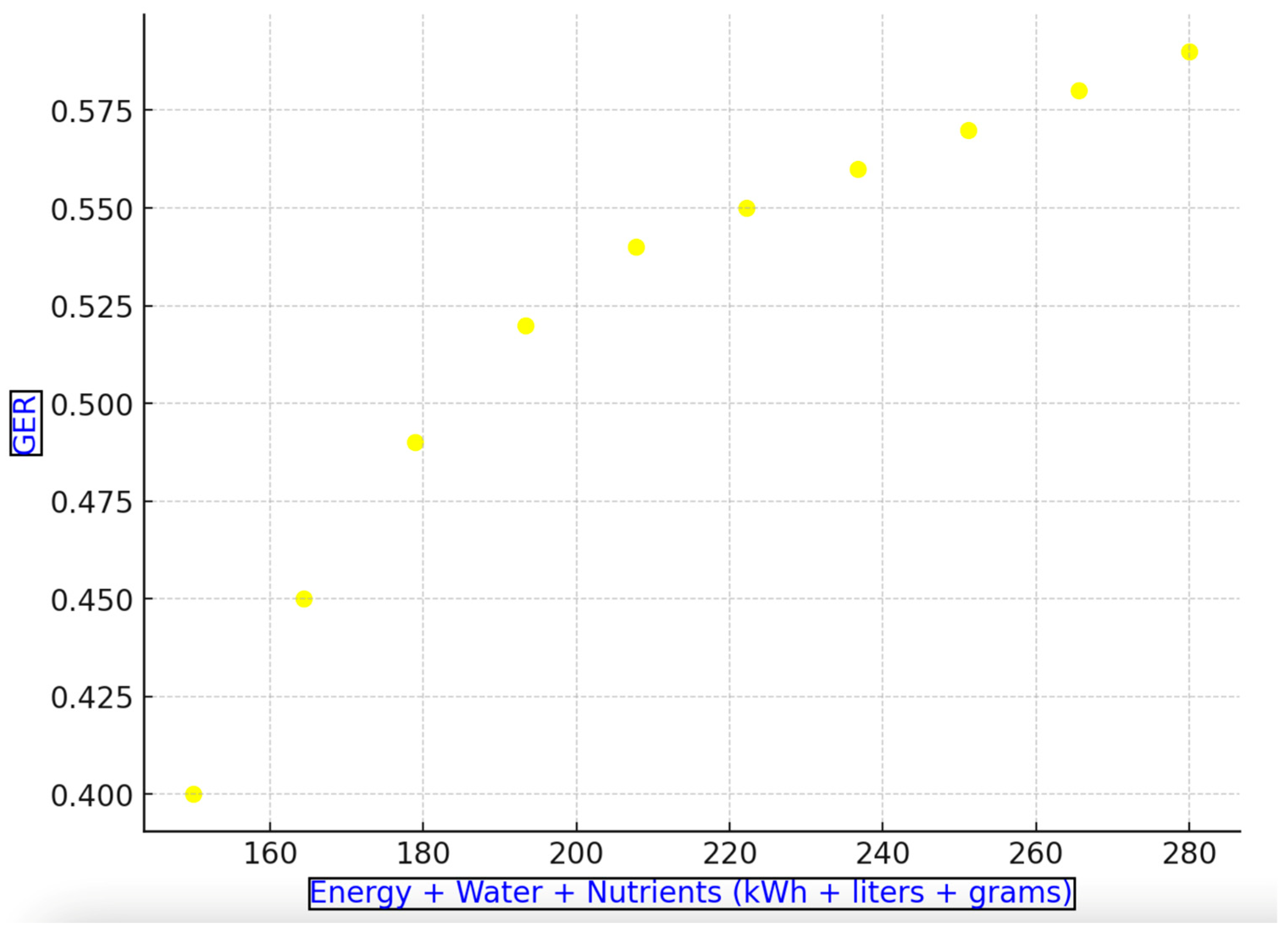
The plot in Figure 7 shows the X-axis representing energy consumption (kWh used per plant or system) and Y-axis representing the Growth Efficiency Ratio (GER), which was calculated as the biomass yield per unit of energy consumed. The data used to plot the graph and to perform the computations of GER values are included in Appendix B 

Table A1. Table for the data used to compute GER over 30 days.

Energy Consumption (kWh)	Water Used (L)	Nutrient Input (g)	Total Biomass Yield (g)	GER
0.8	160	50	64	0.400
1.0	180	55	81	0.450
1.2	200	60	100	0.500
1.4	220	65	115	0.525
1.6	240	70	132	0.550
1.8	260	75	149	0.575
2.0	280	80	162	0.580

.

The plot demonstrates the relationship between combined daily resource used: Energy consumption (kWh), Water usage (L), and Nutrient input (g) and the Growth Efficiency Ratio (GER), that represents the biomass yield per unit of resource consumed. We can observe in the plot that initially, as combined resource input increases, GER also rises, indicating improved efficiency in resource utilization. However, beyond a certain point (approximately 200 units), the rate at which GER increases starts to slow, showing the classic “diminishing returns” effect. This observation suggests that while an initial investment in resources improves growth efficiency, excessive inputs yield minimal benefits to the plant growth. Identifying the values of the threshold allowed us for optimizing resource usage to avoid waste, this is particularly important for cost-effective controlled environment agriculture for our case study.

The plot demonstrates a non-linear relationship, which was mathematically modeled using a polynomial equation, as shown in Equation (13). This equation was derived based on the observed quadratic behavior of GER as a function of combined resource input:

$$\mathrm{GER}=\mathrm{a} (\mathrm{Combined} \mathrm{Resource} \mathrm{Use}{)}^2 + \mathrm{b} (\mathrm{Combined} \mathrm{Resource} \mathrm{Use}) + \mathrm{c}$$

(13)

• Combined Resource Use is the sum of energy consumption (kWh), water usage (L), and nutrient input (g).
• a, b, and c are coefficients determined by fitting the equation to the data.

The coefficients a, b, and c were obtained by performing polynomial regression on the data points in our plot. The values of a, b, and c define the curve’s shape and allowed us to predict GER based on varying levels of combined resource use.

• In our case study, the regression analysis yielded:

• a = −1.198 × ${10}^{-5}$
• b = 0.006474
• c = −0.2924

Then the equation becomes:

$$\mathrm{GER}=-1.198 \times {10}^{-5} (\mathrm{Combined} \mathrm{Resource} \mathrm{Use}{)}^2 + 0.006474 (\mathrm{Combined} \mathrm{Resource} \mathrm{Use}) - 0.2924.$$

(14)

Equation (14) can be used for other case studies, and the concept of “Combined Resource Use” can be generalized to other case studies by adapting the relevant input resources in different systems or plants. To find the maximum level of Growth Efficiency Ratio (GER) based on our polynomial equation, and also to determine the point where adding more inputs becomes inefficient:

Since the equation is a quadratic equation, the maximum GER occurs at the vertex of the parabola. For a downward-opening parabola if a is negative, which implies diminishing returns, the vertex gives the maximum point.

To find the vertex we solve the equation shown in Equation (15):

$$\mathrm{Combined} \mathrm{Resource} {\mathrm{Use}}_{\max }=-{\displaystyle \frac{\mathrm{b}}{2\mathrm{a}}}$$

(15)

This gives the level of combined resource use that maximizes GER. We substitute this value back into the equation to obtain the maximum GER.

We can find the level of resource input where adding more inputs does not lead to significant efficiency gains. We analyze the rate of change of GER by finding the second derivative of the GER equation shown in Equation (16):

$${\displaystyle \frac{d^2\left(GER\right)}{d{\left(Combined Ressource \right)}^2}}=2a$$

(16)

Since a is constant, it confirms that the graph is concave. Negative a means diminishing returns, and to find the point where we should stop adding inputs, we used a threshold approach based on practical significance or efficiency. We observe that when the increase becomes very small, we start at the Combined Resource ${\mathrm{Use}}_{\max }$ value, then we add small values of the inputs to observe when the increase becomes very small. We calculate the GER values in increments at 5 or 10 units above the maximum resource level, until the difference in GER is less than 0.01.

This approach helps us to decide when adding more resources has little impact on GER, indicating an efficient stopping point. In our case study, the Combined Resource $Us{e}_{max}$ is 200 units. We calculated the GER values at 210, 220 and 230 to see when the difference is very small. We found that the GER difference between 210 and 220 was 0.012, but between 230 and 240 was 0.008, therefore 230 units was our stopping point. The value of 230 units is the combined resource use level in our case study beyond which adding more light, water, or nutrients does not lead to meaningful gains in GER for lettuce. At this value, we have to stop adding more resources to avoid inefficient resource usage. This stopping point represents the threshold of diminishing returns, balancing yield with resource efficiency.

3.1.2. GER Heatmap

To further examine how individual resources influence GER, we examined the interaction between light intensity and water usage through additional visualizations. We extended our analysis to understand how individual resource inputs interact to affect GER. Specifically, we examined the combined effects of light intensity and water usage on plant growth efficiency. To visualize these interactions, we generated a heatmap plot illustrating how GER varies across different levels of light and water inputs.

The heatmap displays GER values for multiple combinations of light intensity and water usage. The data used to plot this graph are included in Appendix B Table A1. Each cell in Figure 8 represents a simulation with a specific value of light and water inputs, and the color gradient indicates the corresponding GER. The representation of the plot in Figure 3 demonstrates regions where GER is optimized, illustrating that moderate levels of light intensity combined with moderate water usage yield the highest growth efficiency.

In the GER heatmap, we observe the impact of varying light intensity and water usage on Growth Efficiency Ratio (GER):

1.

Low Light Conditions: The highest value of GER is with low light and medium water use (around 10–12 L), reaching values between to 0.575–0.600. This signifies that, under low light and moderate water levels, the growth efficiency is optimized.

2.

Medium Light Conditions: GER decreases as both light intensity and water usage increase. The highest GER values in medium light are observed at 10 L of water, where GER is around 0.525. Increasing water to 12 L or more in medium light leads to a decrease in GER to values between 0.500–0.525. Therefore, excessive water under medium light does not improve growth efficiency significantly and results in diminishing returns.

3.

High Light Conditions: GER values are lowest under high light and higher water levels (12–15 L), with GER around 0.425–0.475. Even with the highest water input (15 L), GER remains low, showing that an increase in both light intensity and water does not lead to better growth efficiency. This illustrates that high resource inputs in these conditions may be inefficient.

In our case study, optimal GER is achieved under low light conditions with moderate water usage, reaching a peak of 0.600 at 10 L of water. The heatmap clearly shows that both insufficient and excessive inputs lead to lower GER, emphasizing the need for balanced resource allocation.

3.2. Coefficient of Performance (COP)

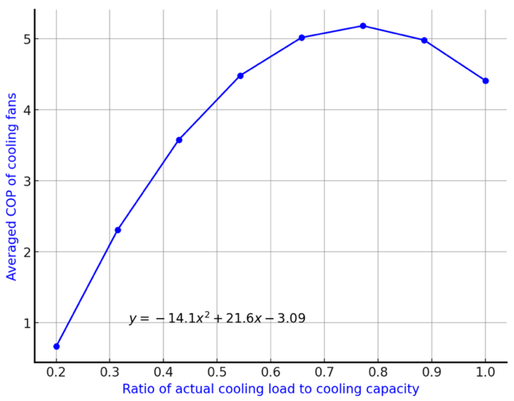
In our case study, the cooling system is ensuring optimal temperature regulation in an indoor environment, which is essential for plant growth. Any indoor plant-growing environment includes fans positioned on either side to circulate air effectively, reducing heat build-up and stabilizing temperature across the room. Temperature control is crucial in enclosed environments to support growth efficiency, as indicated by the Coefficient of Performance (COP) measurements. The Coefficient of Performance measures the efficiency of the cooling fan, defined as the amount of cooling provided per unit of energy consumed. A higher COP indicates better efficiency, as more cooling is achieved with less energy being used. The graph below in Figure 9 shows the relationship between the Coefficient of Performance (COP) of the cooling fans and the ratio of actual cooling load to cooling capacity. The data were generated from controlled environment simulations performed under varying ratios of cooling load to cooling capacity. The raw data are provided in Appendix B 

Table A2. Data of the simulation of COP values according to the ratio of cooling.

Ratio of Actual Cooling Load to Cooling Capacity	Averaged COP of Cooling Fans
0.2	1.296
0.3	2.511
0.4	3.576
0.5	4.491
0.6	5.256
0.7	5.871
0.8	6.336
0.9	6.651
1	5.716

.

The peak COP value occurs between a Cooling Load Ratio of 0.6 and 0.8. In this range, the COP reaches its maximum, indicating that the cooling fan is being efficient, where the fan provides maximum cooling per unit of energy consumed. We solved the equation to find the cooling fan load ratio that provides the best balance, maximizing efficiency without pushing the system to full capacity, where efficiency begins to drop. Solving equation gives that the Cooling Load Ratio that maximizes the COP is approximately 0.77. At this ratio, the COP reaches its peak value of about 5.18. Beyond this point, as the cooling load ratio approaches 1, the COP starts to decline, indicating diminishing efficiency effect when the system is operating at full capacity.

In our case study, the analysis suggests that maintaining a cooling load ratio of around 0.77 achieves maximum efficiency, balancing cooling effectiveness with energy consumption.

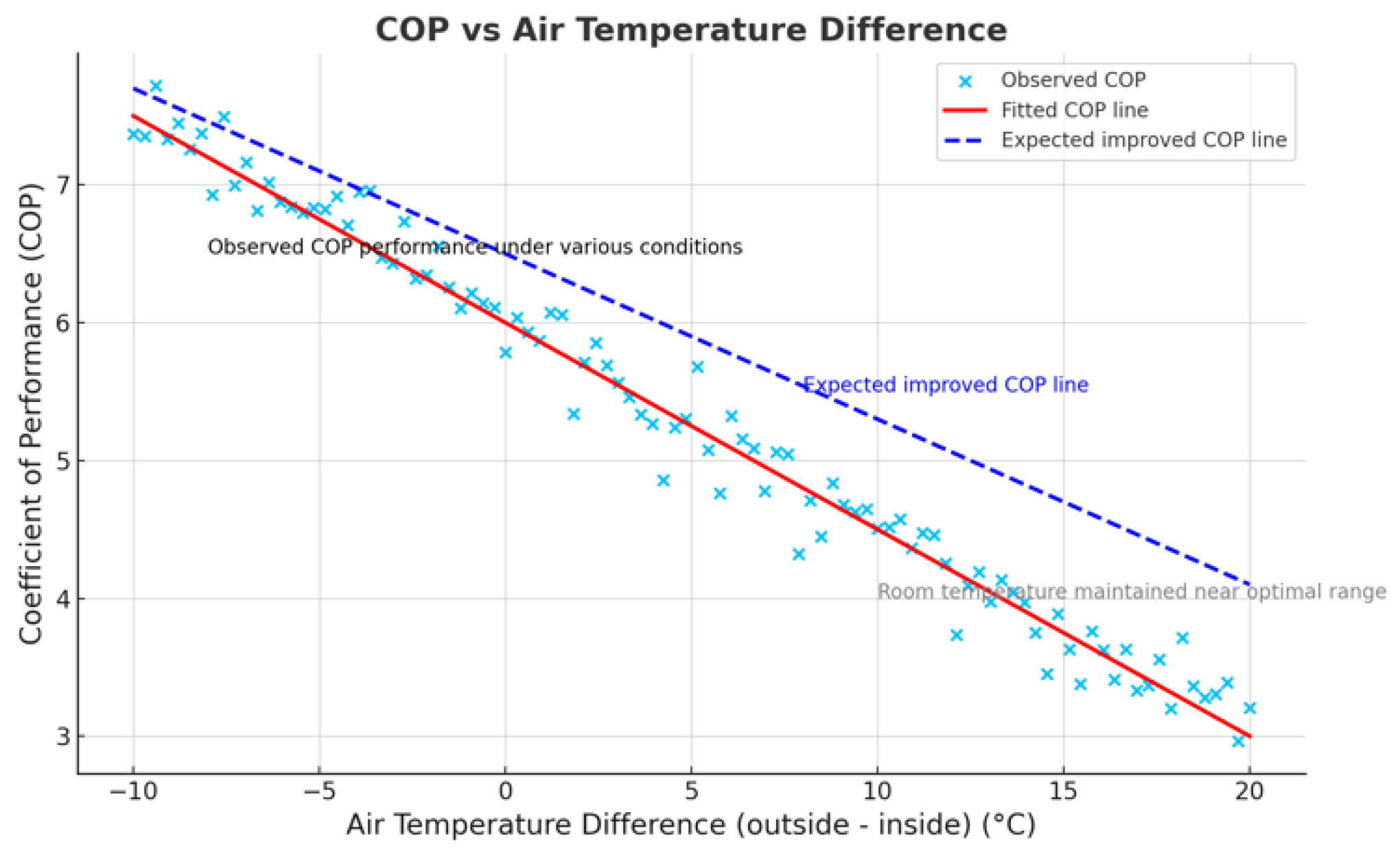
The graph in Figure 10 demonstrates the COP’s relationship with the cooling load ratio and air temperature difference, indicating that the cooling system reaches peak efficiency at a specific range of load and temperature conditions. It illustrates how COP varies with the air temperature difference between the outside and inside environments. The data used to plot the graph are in Appendix B 

Table A3. Table for the calculations of the curves of expected improved cop, fitted cop and observed cop.

${\mathit{T}}_{\mathit{o}\mathit{u}\mathit{t}\mathit{s}\mathit{i}\mathit{d}\mathit{e}}$ (°C)	${\mathit{T}}_{\mathit{i}\mathit{n}\mathit{s}\mathit{i}\mathit{d}\mathit{e}}$ (°C)	$\mathbf{\Delta }\mathit{T}={\mathit{T}}_{\mathit{o}\mathit{u}\mathit{t}\mathit{s}\mathit{i}\mathit{d}\mathit{e}}-{\mathit{T}}_{\mathit{i}\mathit{n}\mathit{s}\mathit{i}\mathit{d}\mathit{e}}$ $\mathit{A}\mathit{i}\mathit{r} \mathit{T}\mathit{e}\mathit{m}\mathit{p}\mathit{e}\mathit{r}\mathit{a}\mathit{t}\mathit{u}\mathit{r}\mathit{e} \mathbf{Difference}$ (°C)	Observed COP	Fitted COP	Expected Improved COP
15	25	−10	6.8	6.7	7.2
20	25	−5	6.0	5.9	6.5
25	25	0	5.2	5.1	5.8
30	25	5	4.3	4.2	4.9
35	25	10	3.5	3.3	4.1
40	25	15	2.8	2.5	3.3
45	25	20	7.5	7.3	7.8

. The blue crosses represent the actual COP values observed at each level of temperature difference. The red line represents the fitted COP line, showing the expected COP performance across varying temperature differences between outside and inside. These data provide insight into how the cooling system performs under different environmental conditions.

As the temperature difference increases, the COP decreases.

• At a temperature difference of around 0 °C, the observed COP is about 6.0, indicating high efficiency.
• When the temperature difference reaches 10 °C, the COP drops to around 4.0.
• At a difference of 20 °C, the COP decreases further to about 3.0.

The graph shows an expected improved COP line, suggesting that maintaining the indoor environment closer to the outdoor temperature within a small difference is beneficial for efficiency.

3.3. Biomass Yield

In controlled environment agriculture, a balance between high biomass yield and resource efficiency is essential to be balanced for the sake of sustainable crop production. Biomass yield reflects the actual growth and productivity of the plants, which is crucial for maximizing output while growing plants indoor. However, producing biomass efficiently measured by the Growth Efficiency Ratio (GER) ensures that resources like water, light, and nutrients are not wasted. Both biomass yield and GER together can give the optimal conditions that provide the highest yield while minimizing resource consumption.

There three important factors that we considered in our study that decide about the growth rate are: Light, Water and Nutrient intake. Therefore, we plotted graphs as shown in Figure 11 combining two parameters at the same time, a bar chart for Biomass yield and a line plot for GER to compare two different parameters from Light, Water and Nutrients on the same graph. The data used for this plot are shown in Appendix B 

Table A4. Table for Biomass Yield and GER across light conditions.

Light (h/Day)	Biomass Yield (g)	GER
6	20	0.47
9	37	0.54
12	45	0.56

.

Our aim was to identify which light condition produces the best balance between high biomass yield and resource efficiency. This is especially useful for decision-making in optimizing resource use.

The bars represent biomass yield in grams under different light conditions: low, medium, and high light conditions. The line plot (GER) indicates the efficiency of biomass production relative to energy consumption or resource use. High light conditions yield the most biomass (around 42 g) and the highest GER (approximately 0.56). However, achieving higher GER with low light conditions is beneficial in our case study as resource efficiency is prioritized over maximizing biomass yield.

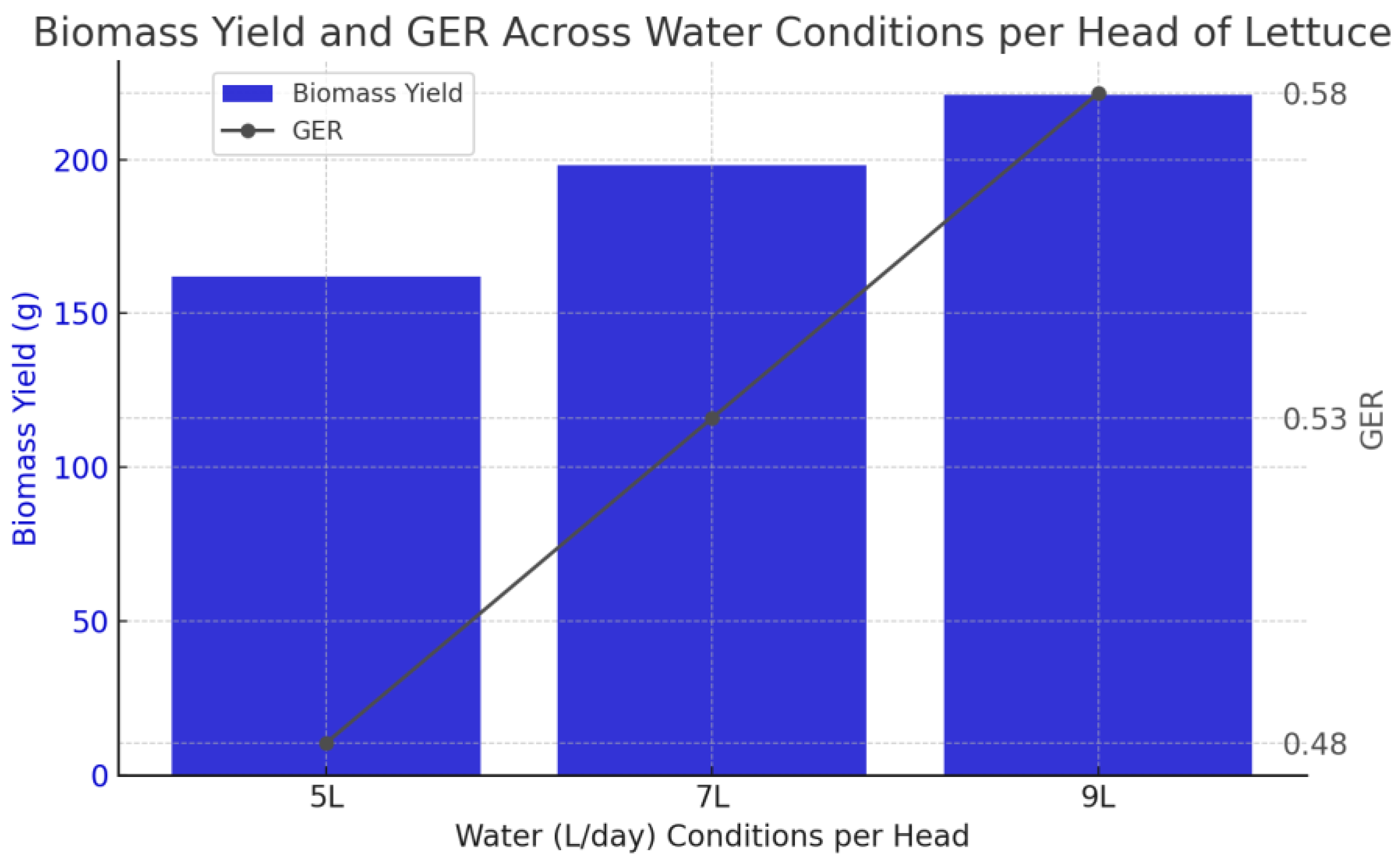
The graph in Figure 12 shows biomass yield and GER at different daily water intake rates (5 L, 7 L, and 9 L per head). The data used for this plot are shown in Appendix B 

Table A5. Table for Biomass Yield and GER across water conditions.

Water (L/Day)	Biomass Yield (g)	GER
5	162	0.46
7	198	0.50
9	221	0.59

. Increased water intake correlates with higher biomass yield, reaching about 210 g at 9 L. GER also improves with increased water usage, reaching about 0.52 at 9 L. This suggests that, within these conditions, higher water intake optimizes both growth and resource efficiency.

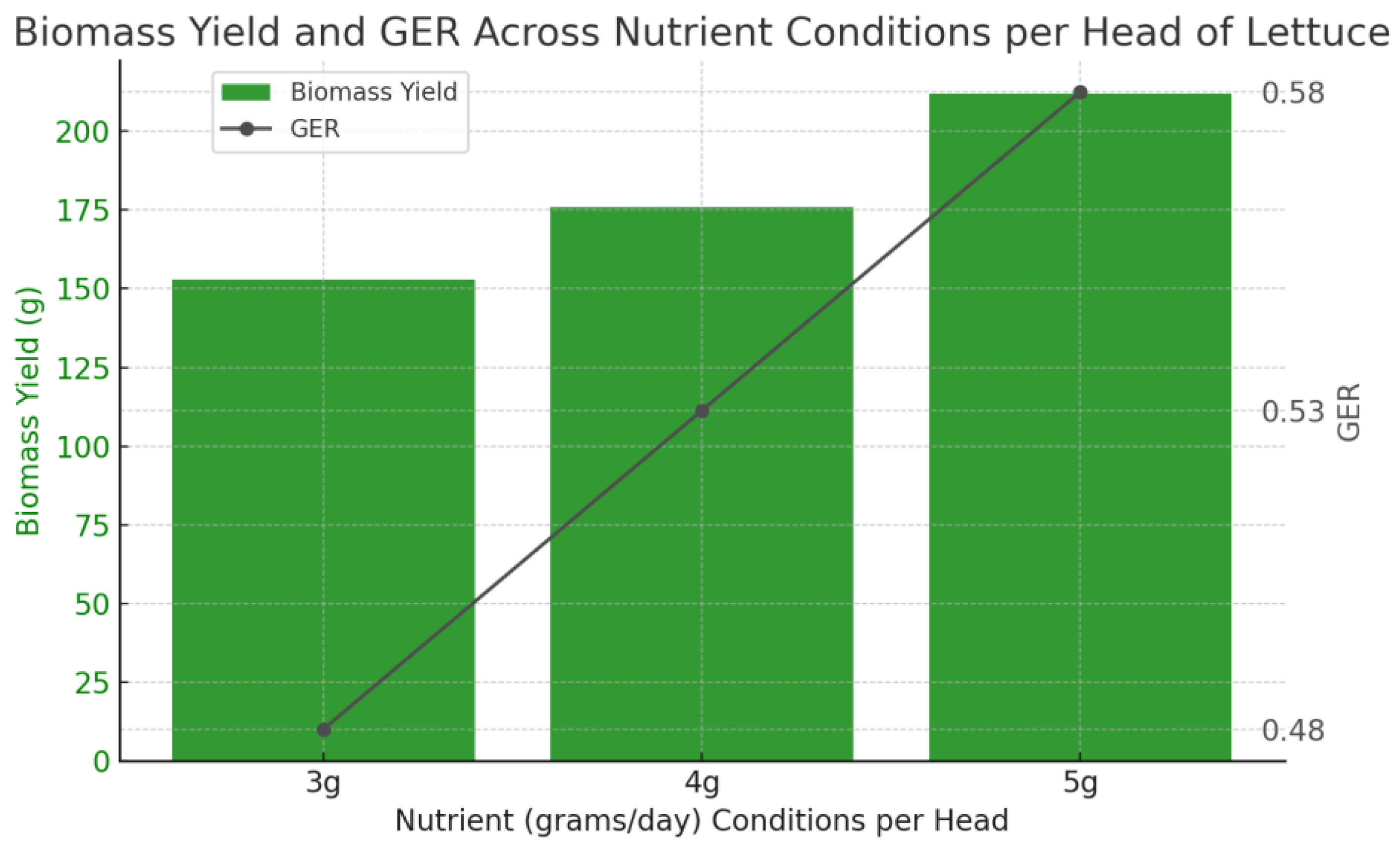
In Figure 13 biomass yield and GER are compared across different daily nutrient intake levels (3 g, 4 g, and 5 g per head). The data used for this plot are shown in Appendix B 

Table A6. Table for Biomass Yield and GER across nutrient conditions.

Nutrient (g/Day)	Biomass Yield (g)	GER
3	153	0.42
4	176	0.51
5	212	0.57

.

Biomass yield peaks at 5 g (close to 200 g), while GER also improves, reaching about 0.51. This indicates that increased nutrient input improves both growth and efficiency, but it is essential to weigh the costs of nutrients against the efficiency gains.

To sum up, from the biomass yield and GER across water conditions plot, 9 L per day appears to yield the highest biomass while still maintaining a high GER. Therefore, 9 L/day seems to be an optimal water level. The biomass yield and GER across nutrient conditions plot suggests that 5 g per day of nutrients provides the highest biomass yield and the best GER. Thus, 5 g/day is optimal for nutrient input. Based on the biomass yield and GER comparison across light conditions and the GER heatmap, high light levels (around 12–14 h of light) seem to support the best growth efficiency and biomass yield. However, medium light conditions (10–12 h) also show efficient GER levels and might be more sustainable for energy use.

3.4. Plant Height

Plant height is a very close parameter to biomass yield, as both metrics reflect the plant’s overall growth and health. Height often correlates with the plant’s ability to capture light and efficiently use water and nutrients, which are essential for biomass production. In controlled environments, analyzing plant height alongside biomass yield provides a more comprehensive view of growth efficiency and productivity. By understanding how changes in light, water, and nutrient inputs affect both height and biomass, we can make data-driven decisions to maximize yield while maintaining resource efficiency.

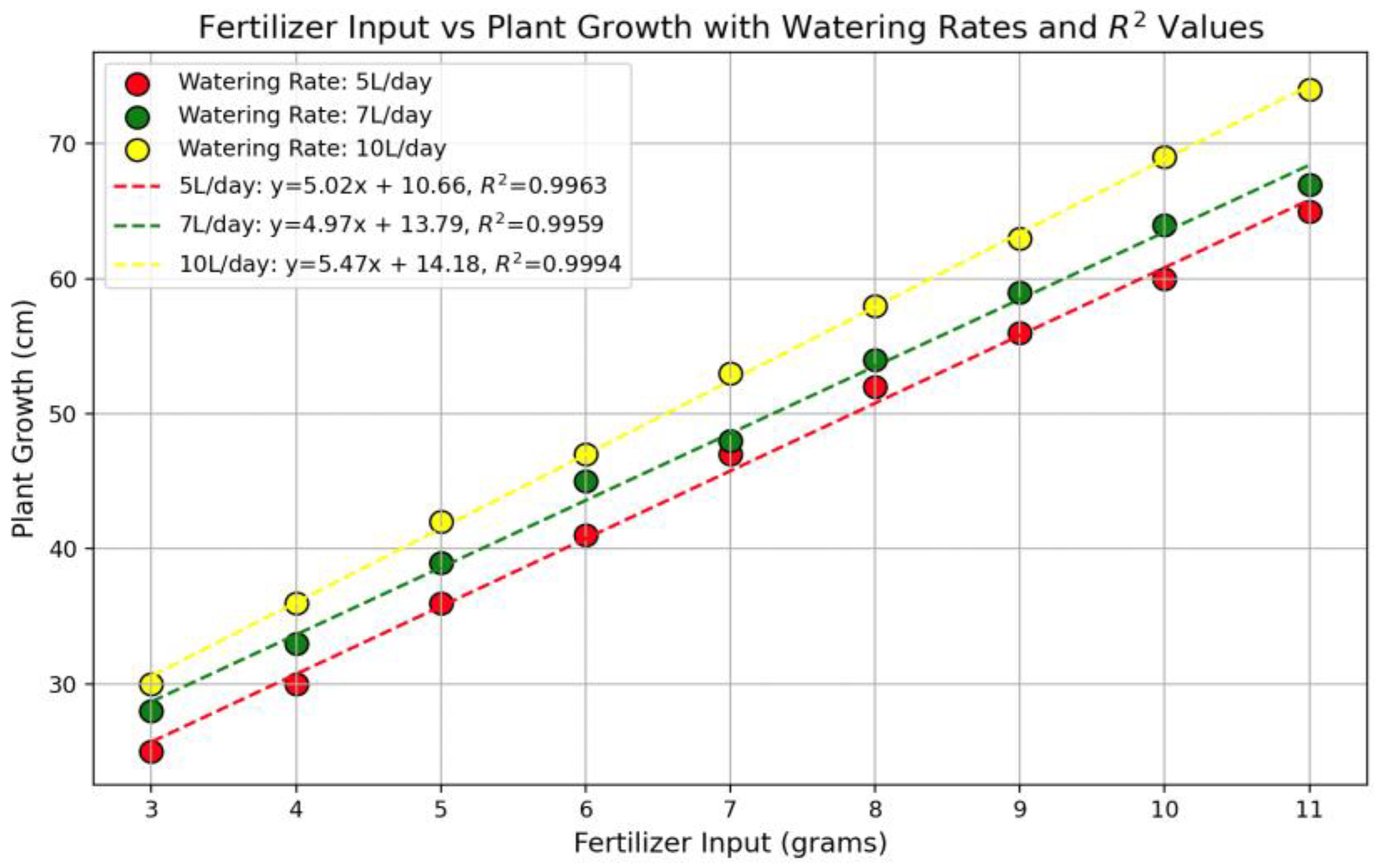
The graph in Figure 14 shows specific quantitative dimensions into how water and nutrient intake impact plant height growth. The data used are shown in Appendix B 

Table A10. Table for the effect of fertilizer input and watering levels on plant growth.

Fertilizer Input (g)	Plant Growth (5 L/Day) (cm)	Plant Growth (7 L/Day) (cm)	Plant Growth (10 L/Day) (cm)
3	25.72	28.7	30.59
4	30.74	33.67	36.06
5	35.76	38.64	41.53
6	40.78	43.61	47.0
7	45.8	48.58	52.47
8	50.81	53.55	57.94
9	55.83	58.51	63.41
10	60.86	63.48	68.88
11	65.88	68.46	74.35

. The slope of each line represents the response of plant height to increasing nutrient levels at each watering rate. Higher slopes indicate a stronger positive response in plant height growth per unit increase in nutrients.

At 10 L/day watering, the slope is higher (5.47), meaning that at this watering rate, plants gain more height per gram of nutrient input compared to the two watering rates.

At 5 L/day watering, the slope is lower (5.02), indicating a less height increase with each additional gram of nutrients.

From the three lines, we observe that higher watering rates lead to better nutrient utilization, and then to greater plant height. This suggests that increasing water from 5 L/day to 10 L/day enhances nutrient uptake efficiency.

For maximizing height growth until plant growth reaches approximately 70 cm, a combination of high watering (10 L/day) with moderate to high nutrient levels (around 9–11 g) appears optimal, given the linear behavior and high slope observed.

The data used are shown in Appendix B 

Table A11. Table for the effect of Light consumption and watering levels on plant growth.

Light Consumption (h)	Plant Growth (5 L/Day) (cm)	Plant Growth (7 L/Day) (cm)	Plant Growth (10 L/Day) (cm)
6	40.02	47.90	53.03
7	45.14	52.01	58.53
8	50.28	57.02	64.06
9	55.42	62.03	69.59
10	60.56	67.04	75.12
11	65.70	72.05	80.65
12	70.84	77.06	86.18
13	75.98	82.07	91.71
14	81.12	87.08	97.24

. Similar to nutrient intake, we observe a positive correlation between light exposure and plant height. As light hours increase, plant height also increases.

At 10 L/day watering, the slope is higher (around 5.53), indicating that plant height grows significantly with each additional hour of light exposure.

At 5 L/day watering, the slope is lower (around 5.14), meaning that the height growth response to light is less effective under reduced watering conditions.

For optimal height growth where the maximum plant growth observed is approximately 90 cm, a combination of 14–15 h of light per day with 10 L/day watering maximizes the efficiency of light in promoting plant height.

These findings in Figure 15 align with our previous results of biomass yield and the Growth Efficiency Ratio (GER), reinforcing the optimal resource allocation we identified. The observed optimal conditions for plant height growth,14–15 h of light exposure combined with a 10 L/day watering rate, correspond with the levels that maximized biomass yield and GER in earlier findings.

3.5. Leaf Area

3.5.1. Leaf Area Development

We used the data from the simulation in the Appendix B 

Table A12. Table for the data of the five leaves starting at different times.

Time (Days from Sowing)	Leaf 1 (Starts Day 10)	Leaf 2 (Starts Day 20)	Leaf 3 (Starts Day 30)	Leaf 4 (Starts Day 40)	Leaf 5 (Starts Day 50)
0	0	0	0	0	0
10	22.01	0	0	0	0
20	105.34	23.12	0	0	0
30	298.75	110.67	25.43	0	0
40	603.89	304.21	109.34	23.98	0
50	801.56	608.73	305.87	110.12	25.78
60	802.31	805.24	607.99	309.45	111.01
70	801.98	802.47	806.12	605.78	308.56
80	802.15	804.76	804.31	807.65	606.21
90	803.24	803.99	805.78	804.12	804.78
100	801.92	802.67	804.45	806.32	802.03

to plot the leaf area versus time after sowing, as shown in Figure 16, to understand the growth progression and the rate at which the individual lettuce leaves are developed.

The graph represents the time-dependent growth of individual lettuce leaves, plotted as the area per leaf (cm²) against days from sowing. Each curve represents a specific leaf that begins development at a distinct point in time, corresponding to the plant’s sequential leaf emergence pattern.

For instance:

• Leaf 1 begins developing around day 10;
• Leaf 2 around day 20;
• Leaf 3 around day 30;
• Leaf 4 around day 40;
• Leaf 5 begins developing around day 50.

Leaves that emerge earlier, such as Leaf 1 (starting around day 10) and Leaf 2 (starting around day 20), benefit from a longer growth period, allowing them to expand fully and achieve their maximum area (~800 cm²) relatively quickly. In contrast, leaves that emerge later, such as Leaf 4 (starting around day 40) and Leaf 5 (starting around day 50), initially grow faster to compensate for the delayed start. However, these later-emerging leaves eventually plateau at a similar maximum area due to genetic limitations and environmental constraints.

Earlier-emerging leaves, such as Leaf 1 and Leaf 2, benefit from stable resources, including light and nutrients, during their growth period, and with minimal competition. In contrast, later-emerging leaves, like Leaf 4 and Leaf 5, face a resource-constrained environment as older leaves occupy more space, intercept light, and utilize nutrients, influencing the growth trajectory of younger leaves. This overlapping growth pattern ensures efficient light interception throughout the plant’s lifecycle, as leaves at different stages contribute to photosynthetic activity. However, the limited leaf area of later-emerging leaves, such as Leaf 5, reflects the plant’s natural balance between maximizing photosynthetic capacity and allocating resources to other essential physiological processes.

3.5.2. Influence of Environmental Factors on Leaf Area

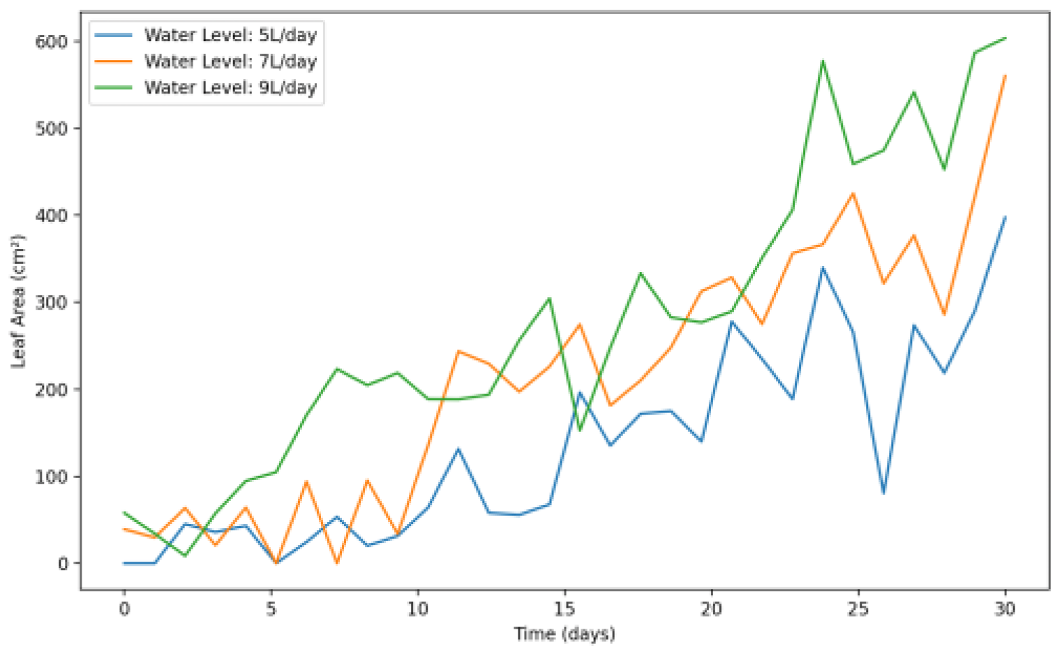
As a part of analyzing the factors impacting the PGI index, we focused on how different environmental factors including water levels, nutrient intake, and light intensity affect the leaf area of plants over a 30-day growth period. Leaf area is a crucial indicator of a plant’s photosynthetic capacity and overall health. Figure 17 shows the change in leaf Area across different water levels, we can see that as water levels increase from 5 L to 9 L per day, there is a clear upward trend in leaf area growth, with 9 L/day yielding the highest leaf area by day 30. The data used to plot this graph are in Appendix B 

Table A9. Data for leaf area growth vs. water levels.

Day	5 L/Day (cm2)	7 L/Day (cm2)	9 L/Day (cm2)
1	30	42	47
5	69	98	129
10	141	192	233
15	212	271	321
20	303	378	453
25	399	503	598
30	521	622	701

.

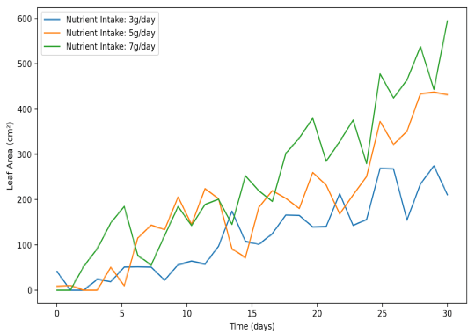
Similar to water levels, increased nutrient intake in Figure 18 shows that a change from 3 g to 7 g per day leads to a larger leaf area. Higher nutrient intake correlates with more significant leaf growth, reaching the maximum around 7 g/day. The data used to plot this graph are in Appendix B Table A10.

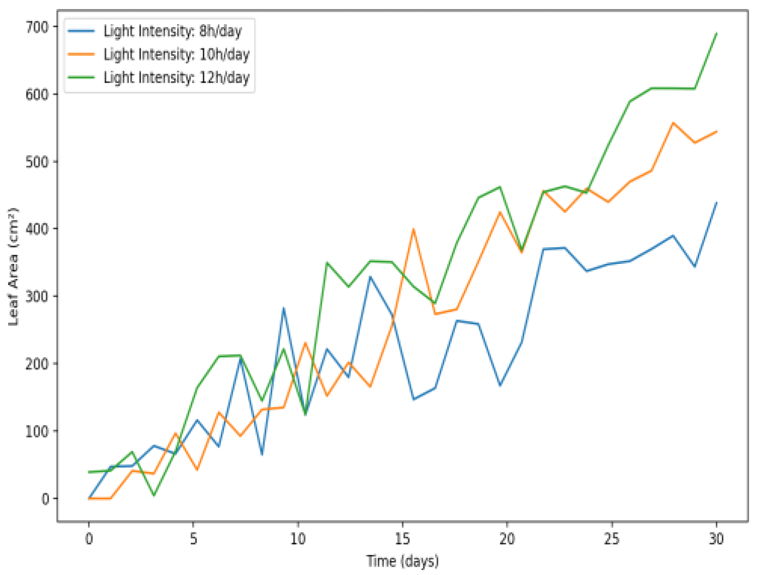
The impact of light exposure shown in Figure 19 is also evident, with higher light intensity (12 h/day) resulting in the most substantial leaf area growth, followed by moderate and low light conditions. The data used to plot this graph are in Appendix B Table A11.

3.6. Machine Learning

To determine the contributions of plant height, biomass, and leaf area to the Plant Growth Index (PGI), we implemented a linear regression model as described in the methodology. The input data are collected iteratively for each data point until the user indicates completion by typing “done”. The Python script is detailed in Appendix A.2. The results, shown in Figure 20, illustrate the input process and the normalized weights.

The normalized weights derived from the linear regression model are as follows:

The highest weight (w2 = 0.55) indicates that biomass has the most significant impact on the PGI. This suggests that biomass accumulation is the primary driver of growth efficiency in the studied plants, likely due to its direct correlation with productivity.

Plant height (w1 = 0.25) contributes moderately, reflecting its role in supporting photosynthetic efficiency and overall structural development.

Leaf area (w3 = 0.20) has a lower contribution, highlighting its supportive role in facilitating photosynthesis but with diminishing returns as leaf overlap and shading occur.

These results emphasize the need to prioritize biomass accumulation strategies, such as nutrient optimization, while monitoring height and leaf area to avoid resource inefficiencies.

3.7. Plant Growth Index (PGI)

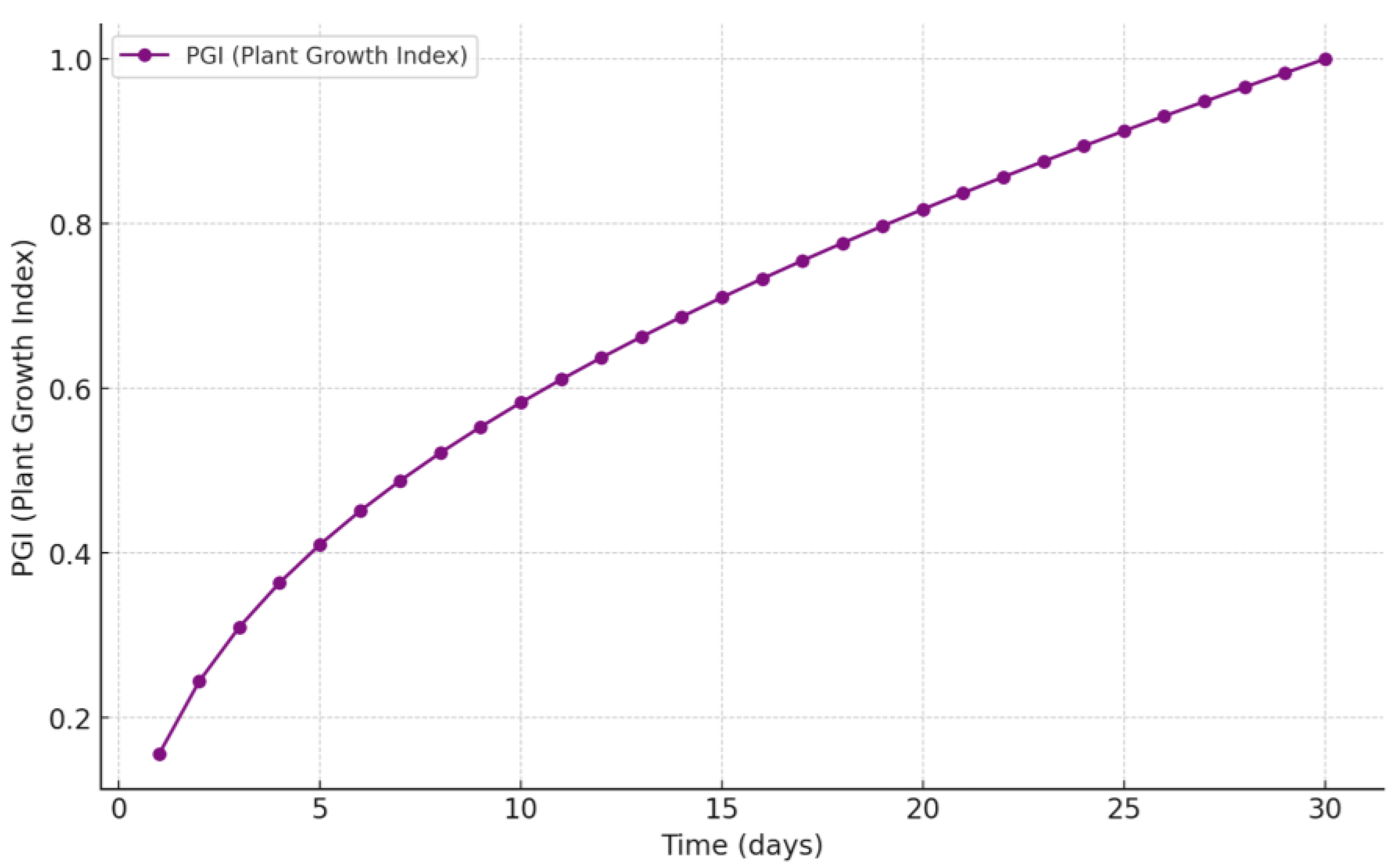
Figure 21 illustrates the progression of the Plant Growth Index (PGI) over a 30-day period. We used the data in the Appendix B 

Table A13. Table of for the raw data for computing the Plant Growth Index (PGI).

Time (Days)	H (cm)	B (g)	A (cm2)	PGI
0	10	20	160	0.20
1	11	22	176	0.23
2	12	24	192	0.26
3	13	26	208	0.29
4	14	28	224	0.33
5	16	32	240	0.37
6	18	36	256	0.41
7	20	40	272	0.45
8	22	44	288	0.49
9	24	48	304	0.53
10	26	52	320	0.57
11	28	56	336	0.60
12	30	60	352	0.63
13	32	64	368	0.67
14	34	68	384	0.70
15	36	72	400	0.73
16	38	76	416	0.76
17	40	80	432	0.79
18	42	84	448	0.82
19	44	88	464	0.85
20	46	92	480	0.88
21	48	96	496	0.90
22	50	100	512	0.92
23	52	104	528	0.94
24	54	108	544	0.96
25	55	110	560	0.97
26	56	112	576	0.98
27	57	114	592	0.99
28	58	116	608	1.00
29	58	116	608	1.00
30	58	116	608	1.00

for the plot. The PGI shows a gradual increase at the start, beginning at approximately 0.2 on Day 0 and reaching 0.6 by Day 10. During this initial phase, plant growth is steady, as resources are being allocated toward early-stage development.

Between Days 10 and 20, the PGI rises more sharply, climbing from 0.6 to 0.8. This phase corresponds to the period of optimal growth, where the plant rapidly accumulates height, biomass, and leaf area under favorable conditions. By Day 20, growth efficiency begins to stabilize, with the PGI continuing to increase at a slower rate until it approaches but never fully reaches its maximum value of 1.0 by Day 30. This indicates that the plant is nearing its growth potential, as defined by the experimental conditions.

The PGI, developed as a novel metric for this study, has proven to be a valuable tool for evaluating plant health and growth efficiency. By combining multiple growth factors (height, biomass, and leaf area) into a single, weighted index, it provides a clear and concise representation of plant performance over time. The metric not only highlights the phases of growth where resource allocation is most effective but also enables informed decision-making for optimizing controlled environment agriculture.

4. Discussion and Conclusions

This study introduces a novel hybrid model that functions as both a model and a framework to enhance plant growth and resource efficiency in controlled environments. As a model, it integrates stochastic, empirical, and optimization to predict plant growth and optimize resource efficiency. As a framework, it applies a logical approach for data collection, analysis, and decision-making, making it adaptable to diverse scenarios and environmental conditions.

The hybrid model combines stochastic modeling, empirical analysis, optimization techniques, and IoT-enabled data collection to enhance plant growth and resource efficiency in controlled environments. By utilizing IoT sensors connected to Raspberry Pi systems, the framework ensured precise and replicable measurements of environmental factors such as light, water, temperature, and humidity, bridging the gap between simulation and real-world applications.

The stochastic model successfully captured environmental variability, while the empirical model quantified relationships between resource inputs and key plant growth metrics, including biomass, height, and leaf area. Machine learning was employed to derive data-driven weights for the Plant Growth Index (PGI), offering a comprehensive evaluation of plant performance. Additionally, the optimization model identified optimal resource levels, resulting in maximum yield and resource efficiency. The framework’s focus on optimizing resource use demonstrated significant environmental benefits. By identifying optimal water usage of 9 L/day, light exposure of 14 h/day, and nutrient input of 5 g/day, the model reduced resource consumption without compromising yields, achieving a maximum biomass of 200 g. Additionally, the cooling system’s optimized Coefficient of Performance (COP) of ~5.18 highlights energy efficiency gains.

Key findings, summarized in

Table 1. Summary of the findings.

Metric	Description	Key Results
Growth Efficiency Ratio (GER)	Efficiency of converting inputs (energy, water, nutrients) into biomass yield.	GER peaked at 0.6 for ~200 units of combined input. Gains beyond 230 units became negligible.
Plant Growth Index (PGI)	Composite index integrating height, biomass, and leaf area, weighted by importance.	PGI increased rapidly from 0.6 to 0.8 (Days 10–20) and saturated at ~1.0 by Day 30.
Cooling Load Ratio (CLR)	Ratio of cooling load to system capacity, measuring fan efficiency.	Maximum efficiency at CLR ~0.77, COP ~5.18.
Plant Height	Vertical growth under optimal conditions.	Maximum height of 90 cm at 14 h light/day and 10 L water/day.
Biomass Yield	Total plant mass in grams.	Maximum biomass of 200 g at 9 L water/day, 5 g nutrients/day, and 14 h light/day.
Leaf Area Dynamics	Growth progression of individual leaves under optimal conditions.	Maximum leaf area per leaf ~800 cm2, with faster initial growth for later-emerging leaves.
Water, Nutrients, and Light Effects	Relationship between environmental inputs and growth metrics.	Optimal inputs: 9 L/day water, 5 g/day nutrients, 14 h/day light.

, highlight the practical relevance of the framework.

Table 1 summarizes our findings from this work:

To conclude, the framework was validated through experimental data and showed significant improvements over traditional models. Previous studies have often relied on single growth metrics, such as biomass yield or plant height, to evaluate performance, which limits their ability to assess resource efficiency comprehensively [34,35]. In contrast, our approach introduced the Growth Efficiency Ratio (GER) and Plant Growth Index (PGI) metrics, which integrate multiple growth factors to provide a more holistic evaluation. This aligns with findings from recent studies [36,37,38], where composite indices were shown to improve decision-making in crop management.

Unlike traditional models that assume constant environmental factors [39,40,41], the stochastic component of this framework accounts for variability in light, temperature, and humidity, offering more realistic simulations. Similar stochastic approaches have been successfully applied in forestry models [42], but their integration with IoT and optimization techniques remains underexplored in agriculture. By incorporating IoT technologies to enhance data accuracy and replicability, this framework addresses critical gaps in precision agriculture [43].

Compared to recent optimization studies [44], which primarily focus on maximizing yield, this framework balances yield with resource efficiency, demonstrating practical applications in resource-limited scenarios. For instance, while previous research on tomato crops identified optimal water use [45], this study extends the approach to a multi-dimensional framework for lettuce cultivation, providing a scalable solution for controlled environment agriculture.

Despite its strengths, the framework has limitations that future research should address. The current model is crop-specific, focusing on lettuce, and further research is required to adapt it to crops with diverse physiological needs. Expanding the framework to include crop-specific parameters and datasets will broaden its applicability. Future studies should also aim to integrate advanced sensors, such as multi-spectral cameras and automated nutrient analyzers, to improve data granularity and model precision.

Finally, the use of linear regression in deriving PGI weights is a limitation, as it restricts the model’s ability to capture complex, non-linear interactions. Incorporating advanced machine learning techniques, such as neural networks, could enhance predictive power and adaptability. By addressing these limitations, the framework has the potential to become a tool for advancing sustainable agricultural practices and improving resource efficiency across a wide range of crops and controlled environment settings