Classification of Plant Leaf Disease Recognition Based on Self-Supervised Learning

Abstract

Accurate identification of plant diseases is a critical task in agricultural production. The existing deep learning crop disease recognition methods require a large number of labeled images for training, limiting the implementation of large-scale detection. To overcome this limitation, this study explores the application of self-supervised learning (SSL) in plant disease recognition. We propose a new model that combines a masked autoencoder (MAE) and a convolutional block attention module (CBAM) to alleviate the harsh requirements of large amounts of labeled data. The performance of the model was validated on the CCMT dataset and our collected dataset. The results show that the improved model achieves an accuracy of 95.35% and 99.61%, recall of 96.2% and 98.51%, and F1 values of 95.52% and 98.62% on the CCMT dataset and our collected dataset, respectively. Compared with ResNet50, ViT, and MAE, the accuracies on the CCMT dataset improved by 1.2%, 0.7%, and 0.8%, respectively, and the accuracy of our collected dataset improved by 1.3%, 1.6%, and 0.6%, respectively. Through experiments on 21 leaf diseases (early blight, late blight, leaf blight, leaf spot, etc.) of five crops, namely, potato, maize, tomato, cashew, and cassava, our model achieved accurate and rapid detection of plant disease categories. This study provides a reference for research work and engineering applications in crop disease detection.

1. Introduction

In modern agricultural practices, rapid and accurate identification of plant diseases is essential for safeguarding crop health, increasing yields, and reducing the use of chemical pesticides [1,2]. However, the variety of disease manifestations and the influence of environmental factors [3] make accurate disease identification a challenge.

Supervised deep learning algorithms have shown good recognition results in current agricultural disease recognition [4,5,6]. On the PlantVillage dataset, the recognition accuracy of different diseases can be up to 95%–99% [7,8]. Li et al. [9] added a coordinate attention (CA) module to the single-stage plant disease network YOLOv5s, as well as key feature weights to enhance the effective information of the feature maps, and the spatial pyramid pooling (SSP) through the data enhancement module was modified to reduce the loss of feature information. Li et al. [10] proposed an improved algorithm for vegetable disease detection based on YOLOv5s which improves the CSP (Cross-Stage Partial), FPN (Feature Pyramid Network), and NMS (non-maximum suppression) modules in YOLOv5s, removes the influence of the external environment, and enhances the ability of multi-scale feature extraction. This improved the accuracy of detection of umbilical rot, gray mold, and cabbage anthracnose on tomato, cucumber, cabbage, and other vegetables. Muhammad et al. [11] recognized leaf spot, powdery mildew, yellow wilt, and other diseases of cotton by meta-deep learning and the accuracy was 98.53%. Ma et al. [12] proposed a lightweight convolutional neural network (CNN) model that can be deployed on mobile terminals to accurately recognize gray leaf spot, common rust, and northern leaf blight of maize with 99.11% recognition accuracy. However, supervised deep learning relies heavily on manual labeling, so we had to find a more efficient solution.

Currently, self-supervised learning in agriculture is increasingly favored [13,14,15], and its learning advantages and good performance in classification tasks are exactly what is needed for plant leaf disease recognition [16]. Self-supervised learning does not require annotation in the traditional sense [17]. Instead, it extracts supervised signals from the input data itself, which means it can learn using unlabeled data. The characteristics of self-supervised learning are very effective when dealing with large amounts of unlabeled data, especially in areas such as disease identification where obtaining labeled data is costly or difficult [18,19]. In addition, mixing self-supervised and supervised methods can improve the performance of the system if there is a large amount of unlabeled data and a small amount of labeled data [20]. Self-supervised learning has been used by scholars for leaf segmentation [21], maturity detection [22,23], growth condition detection [24,25], seed identification [26], and other research directions in plants, which has injected new vigor and vitality into agricultural development.

An MAE (masked autoencoder) [27] is a type of self-supervised learning that is commonly used in the field of image processing. It is an autoencoder-based [28] structure specifically designed to efficiently learn a representation of an image. The key idea is to mask parts of the image and then train the model to reconstruct these masked parts. During the training process, the model learns to minimize the reconstruction error, and in this way the encoder is forced to learn the important feature representations in the image so that it can efficiently reconstruct the masked portions with the help of the decoder [29].

This study focuses on exploring and evaluating the application of self-supervised learning models to the task of plant disease recognition and classification. We employed state-of-the-art self-supervised learning architectures, such as MAE and attention modules (e.g., CBAM), which not only improve recognition accuracy but also enhance the model’s ability to understand disease features. Our experimental results show that through self-supervised learning, the model achieves significant performance improvement on several standard datasets, confirming the great potential of self-supervised learning in solving real-world problems. In addition, our study demonstrates the advantages of self-supervised learning in the case of dealing with limited labeled data, providing new perspectives for future research directions and agricultural practices.

2. Materials and Methods

2.1. Datasets

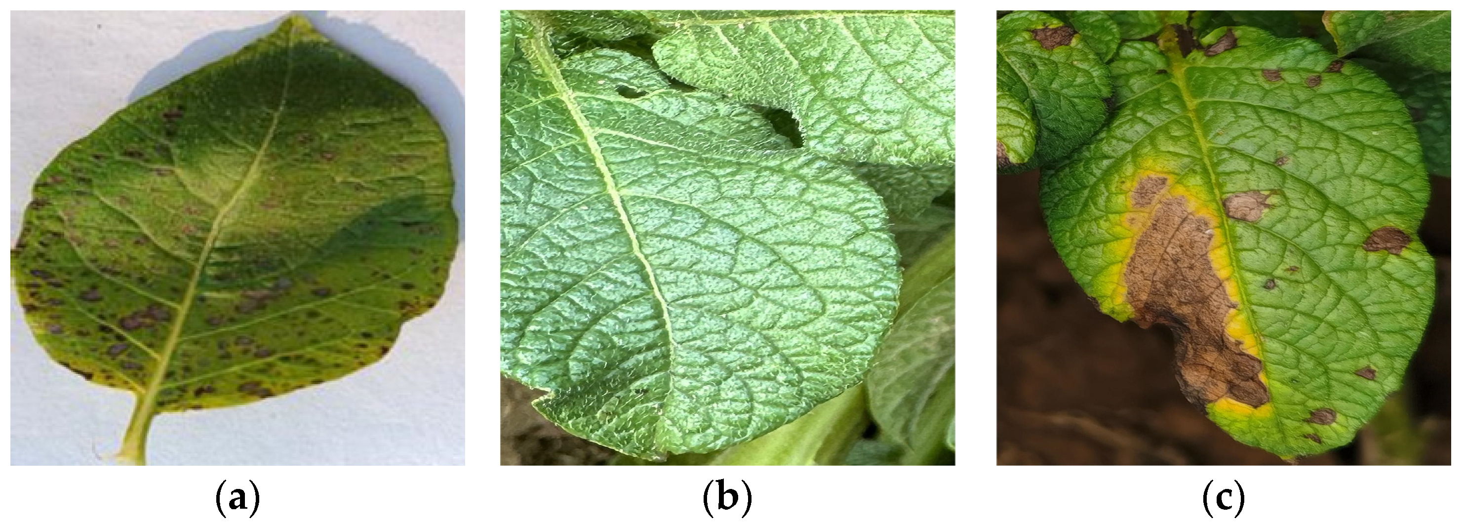
2.1.1. The Dataset We Collected

The dataset we collected was derived from the PLD dataset [30] and images taken and collected by the group at the Yuzi Organic Dry Farming Experimental Site (112°86′ E, 37°76′ N) (Figure 1). The dataset consisted of 3256 images divided into three categories: late blight, early blight, and healthy (

Table 1. Summary of the potato dataset.

Class Labels	Samples
Early_Blight	1628
Healthy	1020
Late_Blight	1692

). We processed our collected dataset by rotating, randomly cropping, and horizontally flipping the original images to increase the size of the dataset.

2.1.2. The CCMT Dataset

CCMT [31] is an open-source dataset for crop diseases, consisting of 88,010 images (23,672 for cashews, 21,768 for cassava, 15,402 for corn, and 27,168 for tomatoes), divided into 18 categories. The dataset includes 18 common leaf diseases such as rust, leaf blight, and leaf spot, as shown in

Table 2. Summary of the CCMT dataset.

CCMT Dataset
Class Labels	Samples	Class Labels	Samples
Cashew_anthracnose	4940	Maize_healthy	1041
Cashew_healthy	7213	Maize_leaf_blight	5029
Cashew_leaf_miner	4953	Maize_leaf_spot	4285
Cashew_red_rust	6566	Maize_streak_virus	5047
Cassava_bacterial_blight	5864	Tomato_healthy	2500
Cassava_brown_spot	4733	Tomato_leaf_blight	6509
Cassava_green_mite	4266	Tomato_leaf_curl	2582
Cassava_healthy	3455	Tomato_septoria_leaf_spot	11,713
Cassava_mosaic	3450	Tomato_verticulium_wilt	3864

. Unlike the PlantVillage dataset, the CCMT dataset images are sourced from field photos and have better adaptability to complex field environments.

2.2. Construction of the Model

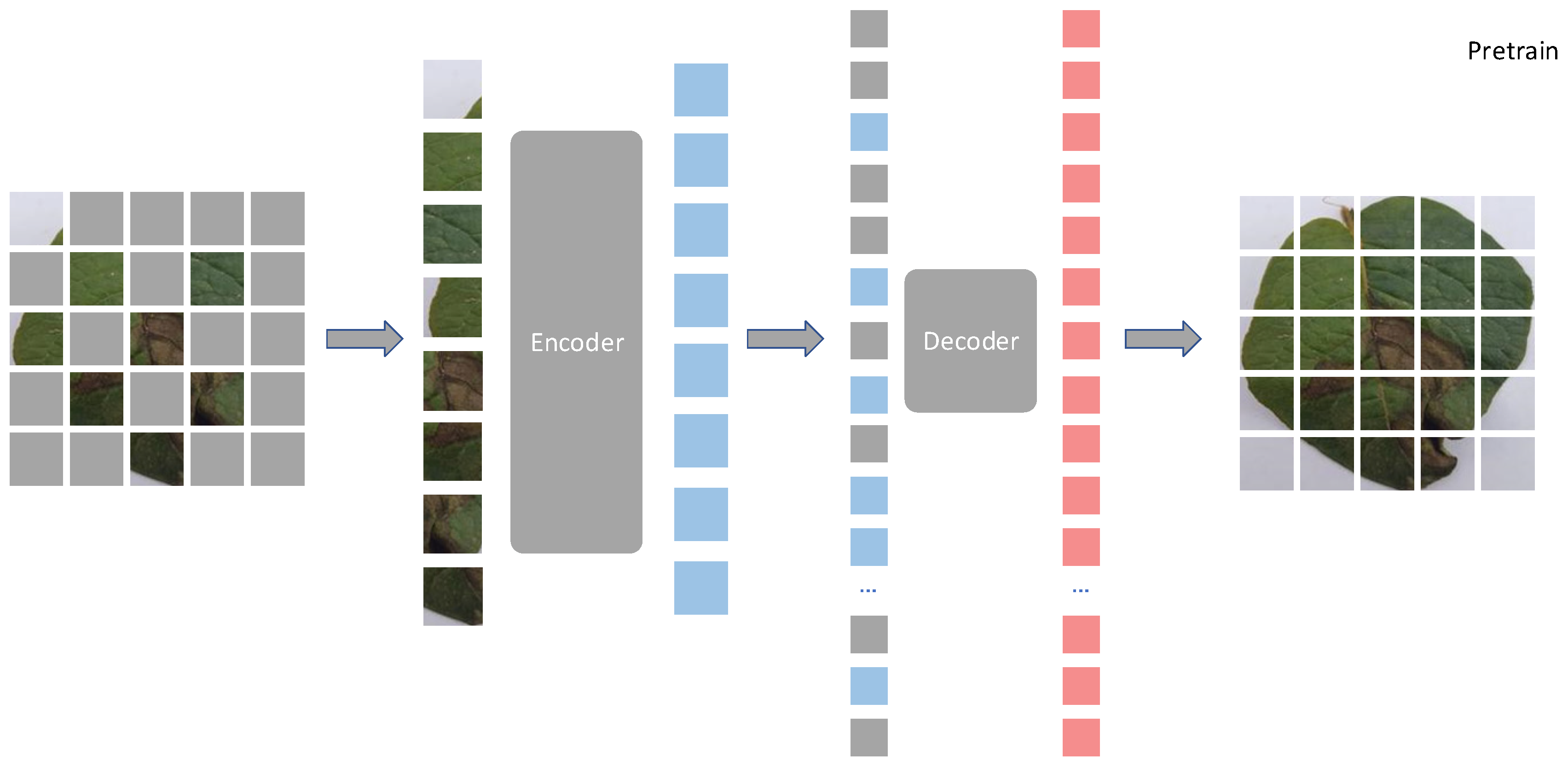
2.2.1. The Masked Autoencoder Model

An MAE (masked autoencoder) [27] is a self-supervised learning algorithm mainly used for visual tasks. It is based on an encoder–decoder architecture (Figure 2) that trains a model by masking parts of the image and trying to reconstruct these masked parts. Blue and red squares are the encoder and decoder outputs respectively MAE is a self-supervised learning algorithm, it does not require a large amount of labeled data for training. It generates the training signals through its own data structures. One of the main advantages of an MAE is its efficient learning process, which reduces the computational burden due to the fact that only some of the pixels need to be processed during the pre-training process. In addition, through the reconstruction task, an MAE is able to capture the global structure and local details of the image, which improves the model’s understanding of the image content.

After the MAE, ViT (Vision Transformer) [32] is used as the backbone structure. In ViT, images are segmented into patches and flattened into patch embeddings, which serve as inputs to the encoder. The encoder of the model consists of N consecutive blocks, each containing mainly of a Multihead Self-Attention (MSA) [33] and a Multilayer Perceptron (MLP) [34] block. ViT employs the Transformer [35] architecture, which is commonly used in natural language processing. This architecture relies on a self-attention mechanism to capture the global dependencies of the input data.

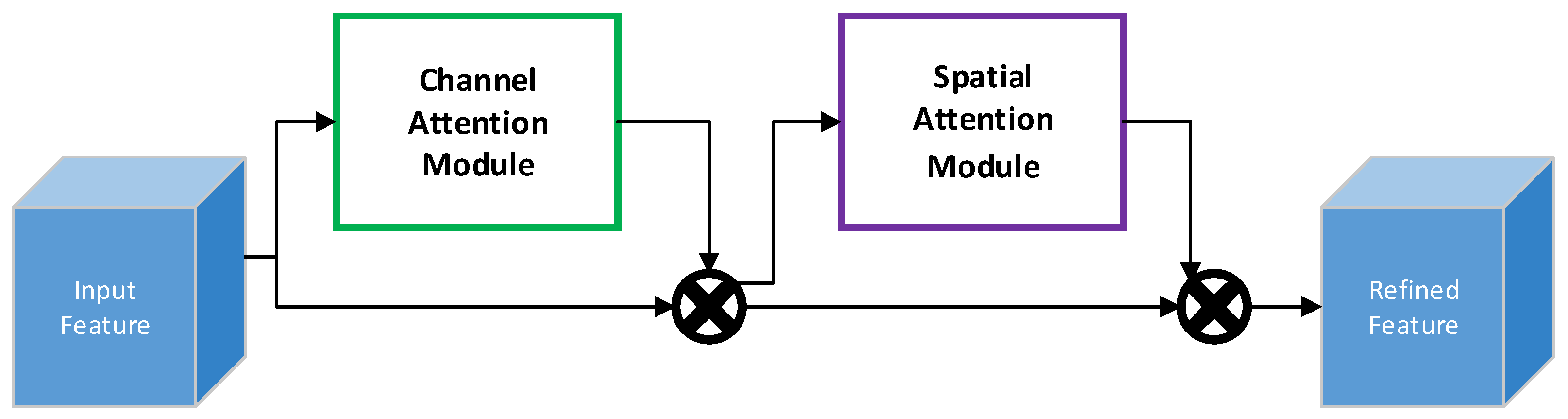
2.2.2. Convolutional Block Attention Module

A CBAM (convolutional block attention module) [36] is an attention mechanism module for convolutional neural networks (Figure 3). This module improves the performance and accuracy of the network by focusing on the most important features in the image [37]. A CBAM mainly consists of two modules, the channel attention mechanism (CAM) and spatial attention mechanism (SAM) modules.

The CAM focuses on determining which channels are important. The importance of each channel is usually computed through global average pooling and maximum pooling operations, followed by a shared network layer. Finally, a channel attention map is generated via a sigmoid activation function, which is used to weight the original feature maps and thus emphasize the important channels.

The SAM focuses on which parts of the image are important. This is usually achieved by performing maximum pooling and average pooling operations (along the channel direction) on the feature maps, which are then stacked together and further processed by a convolutional layer. Similarly, a final spatial attention map is generated through a sigmoid activation function, which is used to weight the original feature map and highlight important spatial regions.

With these two attention mechanisms, the model’s ability to capture important features can be effectively enhanced. Channel attention helps the model to focus on useful feature channels, while spatial attention directs the model to focus on key spatial regions of the image. The combined use of these two classes enables the CBAM to focus on both important channels and spatial regions in the input feature map. This progressively refined attention mechanism improves the model’s sensitivity to important features and thus improves performance.

2.2.3. Gate Recurrent Unit Module

A GRU (Gate Recurrent Unit) [38] is a type of recurrent neural network (RNN) [39]. It was proposed to solve problems such as long-term memory and gradient in backpropagation. Compared to LSTM, the use of a GRU can achieve comparable results [40] and is easier to train, which can largely improve the training efficiency, so it will often be preferred [41].

The GRU controls the flow of information through two gates (update gate and reset gate). The update gate helps the model decide how much of the previous memory to retain in the current state, while the reset gate decides how to combine new input information with past memories. At each time step, the GRU uses the gating mechanism to update its hidden state, and this updated hidden state captures information about the sequence so far. The structural design of the GRU helps to alleviate the problem of gradient vanishing that is common in traditional RNNs by making it capable of learning long-distance dependencies. The formulation of the GRU is as follows (Equation (1)).

$$\begin{array}{c}{z}_t=\sigma \left(W_z\cdot \left[h_{t-1},x_t\right]\right)\\ r_t=\sigma \left(W_r\cdot \left[h_{t-1},x_t\right]\right)\\ \stackrel{\sim }{h_t}=\tanh \left(W\cdot \left[r_t\ast h_{t-1},x_t\right]\right)\\ h_t=\left(1-z_t\right)\ast h_{t-1}+z_t\ast \stackrel{\sim }{h_t}\end{array}$$

(1)

where $x_t$ is the information entered at the current moment; $h_{t-1}$ is the hidden state that represents the previous moment; $h_t$ is the hidden state passed to the next moment; $\stackrel{\sim }{h_t}$ is a candidate hidden state; $r_t$ is a reset gate; $z_t$ is the update gate; $\sigma$ is the sigmoid function by which data can be changed to values in the range 0–1; and $\tanh$ is the tanh function by which data can be changed to values in the range [−1,1].

2.2.4. Improved Model Architecture

We improved the structure of the MAE model by combining the CBAM attention mechanism and GRU. First, we added a CBAM (Figure 4) for feature enhancement of the images before the image blocks enter the encoder. Second, we added the GRU module after the linear layer of the decoder to capture the sequential relationship between the diseased image blocks and enhance the processing of temporal information of the features passed from the encoder.

When processing an image, ViT splits the image into a series of image blocks. These image blocks are feature-enhanced by the CBAM, and each image block is spread and converted into a series of vectors which are subsequently fed into the Transformer model.

The decoder consists of multiple decoding blocks, each containing a Multihead Self-Attention (MSA) [33] and a Multilayer Perceptron (MLP) [34] block. The work of the decoder begins with receiving the output of the encoder, which contains a compressed representation of the unmasked input and a mask token for the masked portion. The decoder uses this information to reconstruct the masked image block. During the training phase, the decoder compares the differences between the minimally reconstructed image and the original image to adjust its parameters. In this way, the decoder not only learns how to accurately fill in the masked portions, but also captures key features of the input data without the need for external labeling. At the same time, our encoder design allows the model to learn complex features inside the image through a self-attentive mechanism, which can subsequently be used for various downstream tasks such as image classification, object detection, or image generation.

2.3. Test Platform and Parameters

The system software used for the test was Windows 11 (64-bit), the programming language was Python version 3.7, Pythorch version 1.14 was used as the processing framework, the deep learning computational framework of Cuda version 16.04 and the cuDNN version 7.6.3 configuration acceleration library were used, and Pycharm was used for debugging the program. The hardware configuration was NVIDIA GeForce RTX 4080 GPU graphics accelerated test process, 16 GB RAM, and 16-core (8P + 8E) 24-thread computer processor with a maximum RX frequency of 5.4 GHz. The size of the training image was adjusted to 256 × 256 pixels, and the batch size of the training was set to 64. The training process consisted of 100 iterations.

Both the CCMT dataset and our collected dataset were divided into training, validation, and test sets in the ratio of 8:1:1. All results are the average recognition accuracy obtained after 5 repetitions of training and testing.

2.4. Evaluation Indicators of Experimental Results

We used Accuracy, Precision, Recall, and F1 score as the evaluation metrics of the model. F1 score is a measure of the precision of a classification model. It is the reconciled average of model Precisionand Recall. The formulas for calculating Accuracy, Recall, Precision and F1 score are given in Equations (2)–(5).

$$Accuracy=\frac{NumberofCorrectPredictions}{TotalNumberofPredictions}\times 100\%$$

(2)

$$Recall=\frac{TruePositives}{TruePositives+FalseNegatives}\times 100\%$$

(3)

$$Precision=\frac{TruePositives}{TruePositives+FalsePositives}\times 100\%$$

(4)

$$F1=2\times \frac{Precision\times Recall}{Precision+Recall}\times 100\%$$

(5)

3. Results

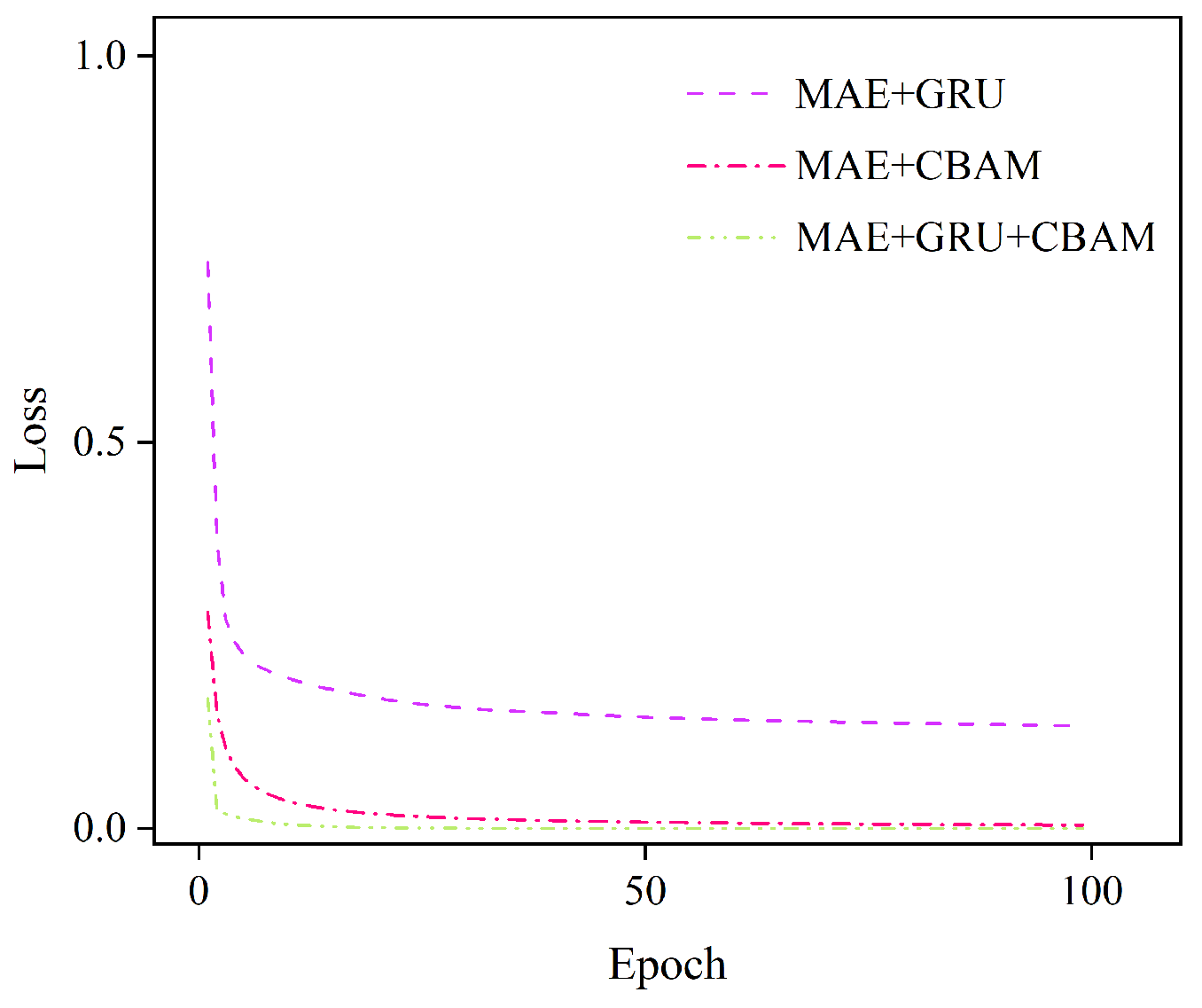
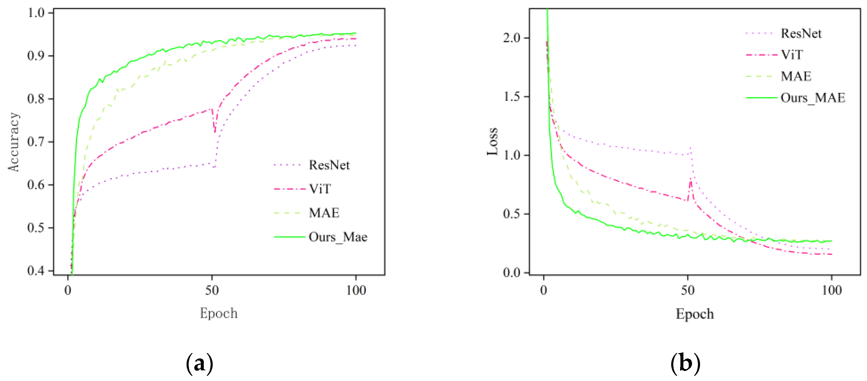
3.1. Comparison and Analysis of Different Improved Models

We added the GRU and CBAM to the MAE model for improving the accuracy and efficiency of the algorithm. Figure 5 shows the loss values of our model pre-trained with the PlantVillage dataset; the model with the addition of the GRU and CBAM has lower loss values and converges faster.

Subsequently, we compared the accuracy of the improved model through experiments on two different datasets. The experimental results are shown in

Table 3. Performance of different improvements on CCMT and our collected dataset.

Dataset	Added Modules	Accuracy	Recall	F1
Our dataset	GRU	98.81%	98.16%	98.17%
	CBAM	98.92%	98.11%	98.10%
	GRU + CBAM	99.35%	98.51%	98.62%
CCMT	GRU	95.29%	96.02%	95.43%
	CBAM	95.17%	95.81%	95.1%
	GRU + CBAM	95.61%	96.20%	95.52%

. On the self-built dataset, the integration of the GRU module resulted in a model with an accuracy of 98.81%, a recall of 98.02%, and an F1 score of 97.98%. Adding the CBAM slightly improves the performance with a 98.92% accuracy, 98.11% recall, and 98.10% F1 score. Combining both the GRU and CBAM performed best on this dataset with a 99.35% accuracy, 98.16% recall, and 98.17% F1 score. Compared to the model with only the GRU and CBAM added, the accuracy of combining both the GRU and CBAM is higher by 0.54% and 0.42%, respectively.

On the CCMT dataset, the GRU module achieved a 95.29% accuracy, 96.02% recall, and 95.43% F1 score. The model using the CBAM scored slightly lower compared to the GRU module, with a 95.17% accuracy, 95.81% recall, and 95.1% F1 score. The combination of the GRU and CBAM again provided the best results with a 95.61% accuracy, 96.20% recall, and 95.52% F1 score. Compared to the model with the addition of the GRU and CBAM only, the accuracy of combining both the GRU and CBAM was 0.32% and 0.44% higher. Therefore, we decided to use the GRU + CBAM model optimization method.

3.2. Comparison and Analysis of the Improved Model with Other Models

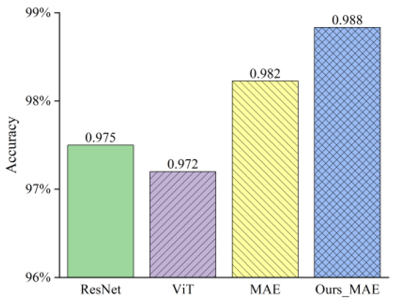
3.2.1. Comparison and Analysis on Our Collected Datasets

The performance of the model is first discussed on the dataset we collected, with the model’s loss function and accuracy curves (Figure 6). As the number of interactions increases, the accuracy of the model steadily increases while the loss continues to decrease. At the beginning of training, the accuracy rises rapidly and the loss decreases rapidly. Subsequently, we compared the improved model with other models on the self-constructed dataset, and three different models (ResNet50, ViT, and MAE) were selected for experiments on the self-constructed dataset (Figure 7). The accuracy of the ResNet50, ViT, and MAE models were 97.5%, 97.2%, and 98.2%, respectively, with Ours_MAE obtaining the highest accuracy (98.8%), which was 1.3%, 1.6%, and 0.6% higher than the other three models, respectively. The accuracy and loss curves of the four algorithms at different epochs are shown in Figure 8.

The normalized confusion matrix in Figure 9 evaluates the model’s performance in a multi-class plant disease recognition task. The results show that the model accurately predicted 99% of the early blight instances, and only 1% of the instances were misclassified as Late_Healthy. Overall, the model showed high accuracy on all three categories, especially in distinguishing early blight from late blight.

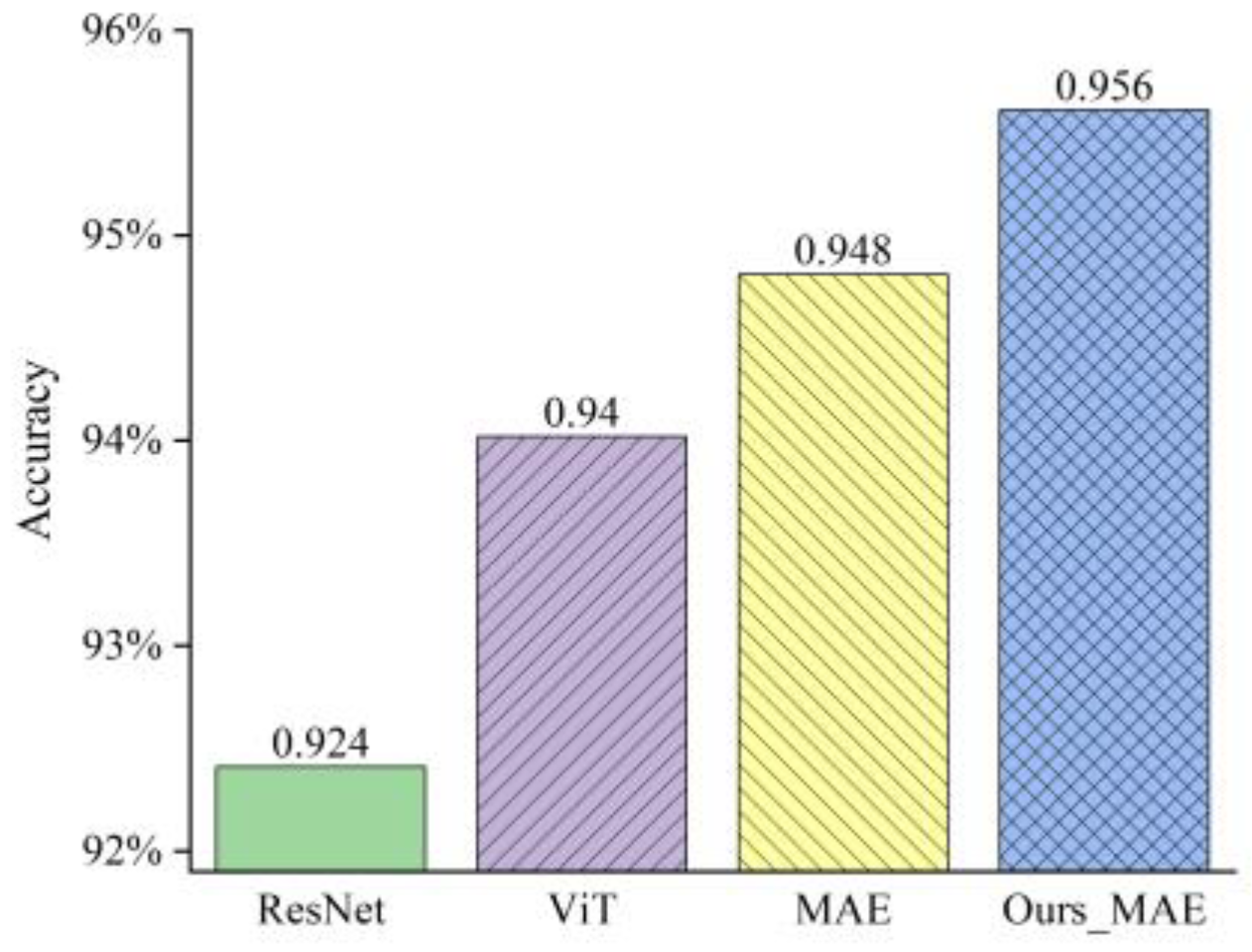
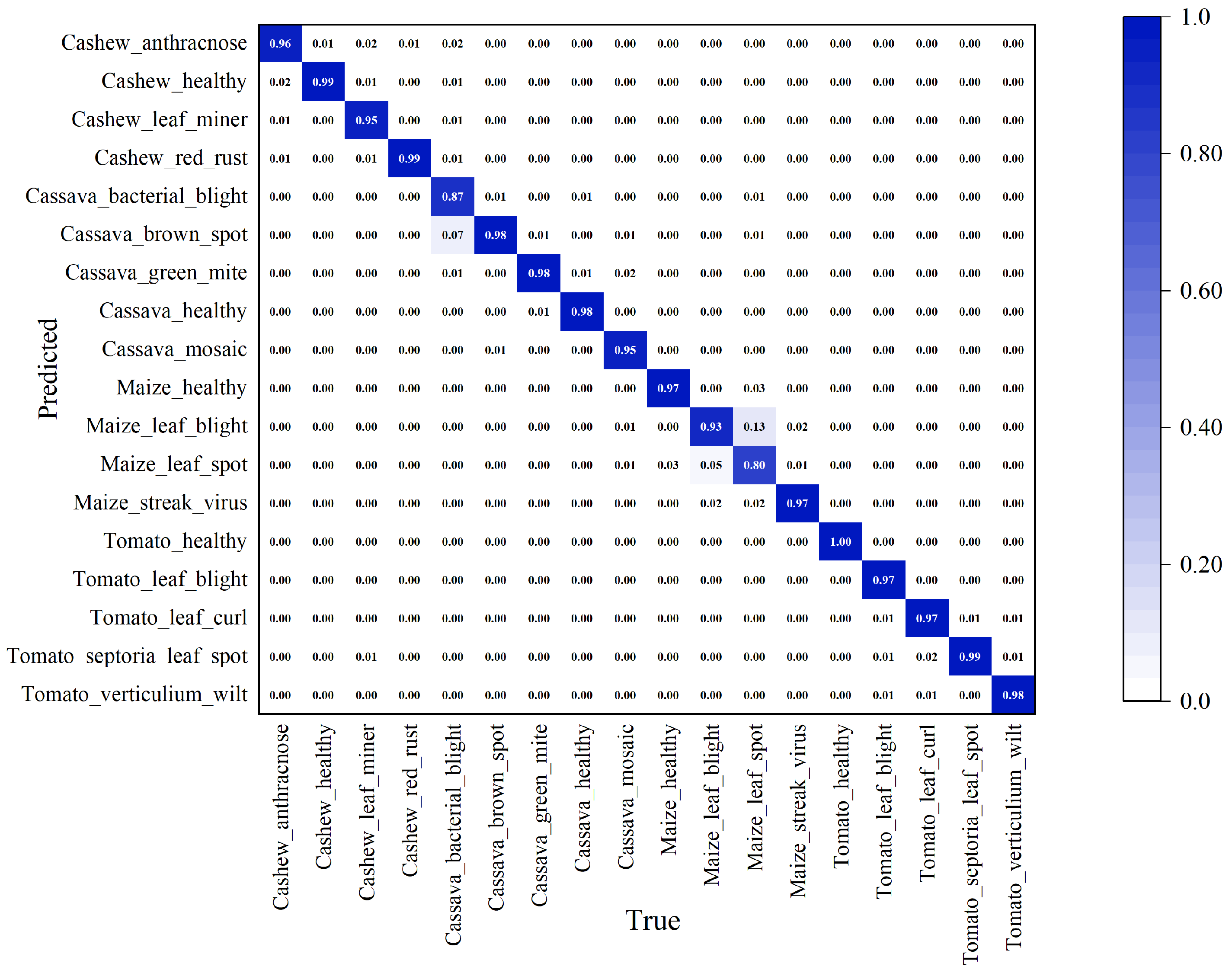
3.2.2. Comparison and Analysis on the CCMT Dataset

In order to evaluate the performance of the models, we selected three different models (ResNet50, ViT, MAE) to test with further experiments on the CCMT dataset, where batch_size was set to 64 and epoch was set to 100 during the training process, and Adma was chosen as the optimizer. Figure 10 shows the accuracy of the ResNet, ViT, and MAE models, which are 98.4%, 94.91%, and 94.81%, respectively. The accuracy of Ours_MAE reaches 95.61%, which is 1.2%, 0.7%, and 0.8% higher than other models, respectively. It can be seen that our model has improved in accuracy.

The accuracy and loss curves of the four models under different epochs are shown in Figure 11 where Ours_MAE has the highest accuracy and a relatively smooth loss curve. The results show that our improved model achieves excellent performance on the CCMT dataset.

In order to analyze the recognition accuracy of our model for different diseases, we analyzed the confusion matrices of the model’s classification predictions, and the normalized confusion matrices of Figure 12 evaluated the model’s performance in the task of recognizing multiple classes of plant diseases. Among them, Cashew_healthy, Tomato_healthy, Cassava_healthy, and Maize_healthy achieved a normalized true-positive rate of more than 0.97, implying that almost all truly healthy plants were correctly classified by the model. Of note, Maize_leaf_spot had a normalized value of 0.13 misclassified as Maize_leaf_blight, indicating some confusion between the two diseases. This provides ideas for further improvement of the model in the future.

4. Discussion

Contrastive learning such as SimCLR [42] and MoCo [43] rely on a comparison of positive and negative sample pairs to learn the representation. These methods learn by maximizing the similarity of positive sample pairs and minimizing the similarity of negative sample pairs [44]. In contrast to this, which typically requires a large number of negative samples and a complex sample selection strategy, an MAE does not rely on sample pair comparisons but on reconstruction tasks, thus avoiding the challenge of needing large-scale negative samples and allowing for training at a much lower computational cost.

The MAE model has several advantages for image classification tasks such as plant disease recognition, including learning global and local features, effective use of unlabeled data, computational efficiency, etc. Once the model captures sufficient feature representations in the pre-training phase, it can be quickly adapted to a specific disease recognition task through a fine-tuning process.

Overall, the MAE model provides a powerful framework for plant disease recognition tasks, especially for situations where data labeling is costly or available labeled data are limited.

The CBAM automatically learns which regions of the image to focus resources on and which feature channels to focus on through channel and spatial attention mechanisms [45]. In disease recognition tasks, this means that the model can automatically highlight diseased spots or damaged regions and ignore background or irrelevant parts. At the same time, CBAM is able to adapt its attention dynamically to different disease types and plant species. The CBAM brings significant performance gains to the plant disease recognition task by providing fine-grained feature adjustment capabilities.

The GRU is a variant of a recurrent neural network (RNN) that is particularly suitable for processing sequence data; although it is not as common as a convolutional neural network (CNN) in processing image data, the GRU can effectively capture disease processes that evolve over time, such as the development and spread of spots, in specific application scenarios describing the development and spread of disease spots. For irregularly shaped disease features, the GRU can handle unstructured data through its recursive mechanism, which helps to recognize and understand complex patterns of disease.

In future research, we will focus on the specific causes of disease occurrence, i.e., whether the disease is caused by different pathogenic factors such as viruses, bacteria, or fungi. Exploration in this direction is important to improve the accuracy and usefulness of plant disease identification. In order to achieve this goal, we need to collect and organize detailed annotated datasets containing different disease causes. The dataset should include different plant species, disease types, and disease manifestations at different stages of development. This should be combined with plant pathology to discover more disease features related to specific pathogens, which can be used as an important basis for model training.

This study demonstrates the application of a self-supervised learning model to the task of plant disease recognition, in particular an approach to enhance model performance by integrating the GRU and CBAM. The results show that the model achieves excellent performance on both the self-built dataset and the CCMT dataset, with a high accuracy, recall, and F1 score. These results can be explained in several ways: firstly, regarding the improvement of the feature learning ability, the GRU module enhances the model’s ability to capture the time series and spatial structure, which is similar to the findings of Bi et al. [46], and the CBAM focuses on key regions in the image through the mechanism of attention, which has been similarly attempted by Alirezazadeh et al. [47], and these help to extract features that are closely related to disease identification. Secondly, regarding the optimization of data utilization, the self-supervised learning framework enables the model to learn useful representations from a large amount of unlabeled data, which reduces the dependence on large-scale labeled datasets, and thus improves the data utilization efficiency. Lastly, regarding the enhancement of the model generalization ability, by pre-training on large-scale datasets, the model learns more general image representations, which improves the model’s ability to generalize in the face of unknown disease types, and similar results were obtained by dong et al. [48].

5. Conclusions

By utilizing a large amount of unlabeled data, this study confirms the potential of self-supervised learning to reduce the reliance on expensive and specialized annotations. This finding is particularly important for the field of agriculture, where data acquisition is costly and specialized knowledge is required. This study not only provides a new technological path for automated identification of plant diseases, but also lays the foundation for further applications of deep learning in agricultural science. We believe that self-supervised learning will play an increasingly important role in the field of plant science with the continuous advancement of computational technology and data processing methods.

References

1. Nigam, S.; Jain, R. Plant disease identification using Deep Learning: A review. Indian J. Agric. Sci. 2020, 90, 249–257. [Google Scholar] [CrossRef]
2. Jin, H.B.; Chu, X.Q.; Qi, J.F.; Zhang, X.X.; Mu, W.S. CWAN: Self-supervised learning for deep grape disease image composition. Eng. Appl. Artif. Intell. 2023, 123, 106458. [Google Scholar] [CrossRef]
3. Zeng, Y.X.; Shi, J.S.; Ji, Z.J.; Wen, Z.H.; Liang, Y.; Yang, C.D. Genotype by Environment Interaction: The Greatest Obstacle in Precise Determination of Rice Sheath Blight Resistance in the Field. Plant Dis. 2017, 101, 1795–1801. [Google Scholar] [CrossRef] [PubMed]
4. Wang, Q.M.; Qi, F.; Sun, M.H.; Qu, J.H.; Xue, J. Identification of Tomato Disease Types and Detection of Infected Areas Based on Deep Convolutional Neural Networks and Object Detection Techniques. Comput. Intell. Neurosci. 2019, 2019, 9142753. [Google Scholar] [CrossRef] [PubMed]
5. Nie, X.; Wang, L.Y.; Ding, H.X.; Xu, M. Strawberry Verticillium Wilt Detection Network Based on Multi-Task Learning and Attention. IEEE Access 2019, 7, 170003–170011. [Google Scholar] [CrossRef]
6. Sunil, C.K.; Jaidhar, C.D.; Patil, N. Systematic study on deep learning-based plant disease detection or classification. Artif. Intell. Rev. 2023, 56, 14955–15052. [Google Scholar] [CrossRef]
7. Khan, A.T.; Jensen, S.M.; Khan, A.R.; Li, S. Plant disease detection model for edge computing devices. Front. Plant Sci. 2023, 14, 1308528. [Google Scholar] [CrossRef] [PubMed]
8. Craze, H.A.; Pillay, N.; Joubert, F.; Berger, D.K. Deep Learning Diagnostics of Gray Leaf Spot in Maize under Mixed Disease Field Conditions. Plants 2022, 11, 1942. [Google Scholar] [CrossRef]
9. Li, Y.; Sun, S.Y.; Zhang, C.S.; Yang, G.S.; Ye, Q.B. One-Stage Disease Detection Method for Maize Leaf Based on Multi-Scale Feature Fusion. Appl. Sci. 2022, 12, 7960. [Google Scholar] [CrossRef]
10. Li, J.W.; Qiao, Y.L.; Liu, S.; Zhang, J.H.; Yang, Z.C.; Wang, M.L. An improved YOLOv5-based vegetable disease detection method. Comput. Electron. Agric. 2022, 202, 107345. [Google Scholar] [CrossRef]
11. Memon, M.S.; Kumar, P.; Iqbal, R. Meta Deep Learn Leaf Disease Identification Model for Cotton Crop. Computers 2022, 11, 102. [Google Scholar] [CrossRef]
12. Ma, Z.; Wang, Y.; Zhang, T.S.; Wang, H.G.; Jia, Y.J.; Gao, R.; Su, Z.B. Maize leaf disease identification using deep transfer convolutional neural networks. Int. J. Agric. Biol. Eng. 2022, 15, 187–195. [Google Scholar] [CrossRef]
13. Jing, L.; Tian, Y. Self-supervised visual feature learning with deep neural networks: A survey. IEEE Trans. Pattern Anal. Mach. Intell. 2020, 43, 4037–4058. [Google Scholar] [CrossRef]
14. Yan, J.; Wang, X.F. Unsupervised and semi-supervised learning: The next frontier in machine learning for plant systems biology. Plant J. 2022, 111, 1527–1538. [Google Scholar] [CrossRef] [PubMed]
15. Zhang, Y.S.; Chen, L.; Yuan, Y. Multimodal Fine-Grained Transformer Model for Pest Recognition. Electronics 2023, 12, 2620. [Google Scholar] [CrossRef]
16. Gong, X.J.; Zhang, X.H.; Zhang, R.W.; Wu, Q.F.; Wang, H.; Guo, R.C.; Chen, Z.R. U3-YOLOXs: An improved YOLOXs for Uncommon Unregular Unbalance detection of the rape subhealth regions. Comput. Electron. Agric. 2022, 203, 107461. [Google Scholar] [CrossRef]
17. Liu, X.; Zhang, F.J.; Hou, Z.Y.; Mian, L.; Wang, Z.Y.; Zhang, J.; Tang, J. Self-Supervised Learning: Generative or Contrastive. IEEE Trans. Knowl. Data Eng. 2023, 35, 857–876. [Google Scholar] [CrossRef]
18. Ohri, K.; Kumar, M. Review on self-supervised image recognition using deep neural networks. Knowl.-Based Syst. 2021, 224, 107090. [Google Scholar] [CrossRef]
19. Yang, G.F.; Yang, Y.; He, Z.K.; Zhang, X.Y.; He, Y. A rapid, low-cost deep learning system to classify strawberry disease based on cloud service. J. Integr. Agric. 2022, 21, 460–473. [Google Scholar] [CrossRef]
20. Tomasev, N.; Bica, I.; McWilliams, B.; Buesing, L.; Pascanu, R.; Blundell, C.; Mitrovic, J. Pushing the limits of self-supervised ResNets: Can we outperform supervised learning without labels on ImageNet? arXiv 2022, arXiv:2201.05119. [Google Scholar]
21. Lin, X.F.; Li, C.T.; Adams, S.; Kouzani, A.Z.; Jiang, R.C.; He, L.G.; Hu, Y.J.; Vernon, M.; Doeven, E.; Webb, L.; et al. Self-Supervised Leaf Segmentation under Complex Lighting Conditions. Pattern Recognit. 2023, 135, 109021. [Google Scholar] [CrossRef]
22. Gai, R.L.; Wei, K.; Wang, P.F. SSMDA: Self-Supervised Cherry Maturity Detection Algorithm Based on Multi-Feature Contrastive Learning. Agriculture 2023, 13, 939. [Google Scholar] [CrossRef]
23. Xiao, B.J.; Nguyen, M.; Yan, W.Q. Fruit ripeness identification using transformers. Appl. Intell. 2023, 53, 22488–22499. [Google Scholar] [CrossRef]
24. Liu, Y.S.; Zhou, S.B.; Wu, H.M.; Han, W.; Li, C.; Chen, H. Joint optimization of autoencoder and Self-Supervised Classifier: Anomaly detection of strawberries using hyperspectral imaging. Comput. Electron. Agric. 2022, 198, 107007. [Google Scholar] [CrossRef]
25. Zheng, H.; Wang, G.H.; Li, X.C. Swin-MLP: A strawberry appearance quality identification method by Swin Transformer and multi-layer perceptron. J. Food Meas. Charact. 2022, 16, 2789–2800. [Google Scholar] [CrossRef]
26. Bi, C.G.; Hu, N.; Zou, Y.Q.; Zhang, S.; Xu, S.Z.; Yu, H.L. Development of Deep Learning Methodology for Maize Seed Variety Recognition Based on Improved Swin Transformer. Agronomy 2022, 12, 1843. [Google Scholar] [CrossRef]
27. He, K.; Chen, X.; Xie, S.; Li, Y.; Dollár, P.; Girshick, R. Masked autoencoders are scalable vision learners. In Proceedings of the IEEE/CVF Conference on Computer Vision and Pattern Recognition, New Orleans, LA, USA, 18–24 June 2022; pp. 16000–16009. [Google Scholar]
28. Wang, S.P.; Cai, J.Y.; Lin, Q.H.; Guo, W.Z. An Overview of Unsupervised Deep Feature Representation for Text Categorization. IEEE Trans. Comput. Soc. Syst. 2019, 6, 504–517. [Google Scholar] [CrossRef]
29. Li, P.Z.; Pei, Y.; Li, J.Q. A comprehensive survey on design and application of autoencoder in deep learning. Appl. Soft Comput. 2023, 138, 110176. [Google Scholar] [CrossRef]
30. Rashid, J.; Khan, I.; Ali, G.; Almotiri, S.H.; AlGhamdi, M.A.; Masood, K. Multi-Level Deep Learning Model for Potato Leaf Disease Recognition. Electronics 2021, 10, 2064. [Google Scholar] [CrossRef]
31. Mensah, P.K.; Akoto-Adjepong, V.; Adu, K.; Ayidzoe, M.A.; Bediako, E.A.; Nyarko-Boateng, O.; Boateng, S.; Donkor, E.F.; Bawah, F.U.; Awarayi, N.S. CCMT: Dataset for crop pest and disease detection. Data Brief 2023, 49, 109306. [Google Scholar] [CrossRef]
32. Arnab, A.; Dehghani, M.; Heigold, G.; Sun, C.; Lučić, M.; Schmid, C. Vivit: A video vision transformer. In Proceedings of the IEEE/CVF International Conference on Computer Vision, Virtual, 11–17 October 2021; pp. 6836–6846. [Google Scholar]
33. Voita, E.; Talbot, D.; Moiseev, F.; Sennrich, R.; Titov, I. Analyzing multi-head self-attention: Specialized heads do the heavy lifting, the rest can be pruned. arXiv 2019, arXiv:1905.09418. [Google Scholar]
34. Tang, J.; Deng, C.; Huang, G.-B. Extreme learning machine for multilayer perceptron. IEEE Trans. Neural Netw. Learn. Syst. 2015, 27, 809–821. [Google Scholar] [CrossRef] [PubMed]
35. Vaswani, A.; Shazeer, N.; Parmar, N.; Uszkoreit, J.; Jones, L.; Gomez, A.N.; Kaiser, Ł.; Polosukhin, I. Attention is all you need. Adv. Neural Inf. Process. Syst. 2017, 30, 6000–6010. [Google Scholar]
36. Woo, S.; Park, J.; Lee, J.-Y.; Kweon, I.S. Cbam: Convolutional block attention module. In Proceedings of the European Conference on Computer Vision (ECCV), Munich, Germany, 8–14 September 2018; pp. 3–19. [Google Scholar]
37. Park, J.; Woo, S.; Lee, J.-Y.; Kweon, I.S. A simple and light-weight attention module for convolutional neural networks. Int. J. Comput. Vis. 2020, 128, 783–798. [Google Scholar] [CrossRef]
38. Dey, R.; Salem, F.M. Gate-variants of gated recurrent unit (GRU) neural networks. In Proceedings of the 2017 IEEE 60th International Midwest Symposium on Circuits and Systems (MWSCAS), Boston, MA, USA, 6–9 August 2017; pp. 1597–1600. [Google Scholar]
39. Medsker, L.R.; Jain, L. Recurrent neural networks. Des. Appl. 2001, 5, 2. [Google Scholar]
40. Shu, W.; Cai, K.; Xiong, N.N. A short-term traffic flow prediction model based on an improved gate recurrent unit neural network. IEEE Trans. Intell. Transp. Syst. 2021, 23, 16654–16665. [Google Scholar] [CrossRef]
41. Zhou, G.-B.; Wu, J.; Zhang, C.-L.; Zhou, Z.-H. Minimal gated unit for recurrent neural networks. Int. J. Autom. Comput. 2016, 13, 226–234. [Google Scholar] [CrossRef]
42. Chen, T.; Kornblith, S.; Norouzi, M.; Hinton, G. A simple framework for contrastive learning of visual representations. In Proceedings of the International Conference on Machine Learning, Virtual, 13–18 July 2020; pp. 1597–1607. [Google Scholar]
43. He, K.; Fan, H.; Wu, Y.; Xie, S.; Girshick, R. Momentum contrast for unsupervised visual representation learning. In Proceedings of the IEEE/CVF Conference on Computer Vision and Pattern Recognition, Seattle, WA, USA, 14–19 June 2020; pp. 9729–9738. [Google Scholar]
44. Wang, X.; Qi, G.-J. Contrastive learning with stronger augmentations. IEEE Trans. Pattern Anal. Mach. Intell. 2022, 45, 5549–5560. [Google Scholar] [CrossRef] [PubMed]
45. Wang, W.; Tan, X.; Zhang, P.; Wang, X. A CBAM based multiscale transformer fusion approach for remote sensing image change detection. IEEE J. Sel. Top. Appl. Earth Obs. Remote Sens. 2022, 15, 6817–6825. [Google Scholar] [CrossRef]
46. Bi, L.N.; Hu, G.P.; Raza, M.M.; Kandel, Y.; Leandro, L.; Mueller, D. A Gated Recurrent Units (GRU)-Based Model for Early Detection of Soybean Sudden Death Syndrome through Time-Series Satellite Imagery. Remote Sens. 2020, 12, 3621. [Google Scholar] [CrossRef]
47. Alirezazadeh, P.; Schirrmann, M.; Stolzenburg, F. Improving Deep Learning-based Plant Disease Classification with Attention Mechanism. Gesunde Pflanz. 2023, 75, 49–59. [Google Scholar] [CrossRef]
48. Dong, X.Y.; Wang, Q.; Huang, Q.D.; Ge, Q.L.; Zhao, K.J.; Wu, X.C.; Wu, X.; Lei, L.; Hao, G.F. PDDD-PreTrain: A Series of Commonly Used Pre-Trained Models Support Image-Based Plant Disease Diagnosis. Plant Phenomics 2023, 5, 0054. [Google Scholar] [CrossRef] [PubMed]
Figure 1. Examples of samples from our potato disease dataset. (a) Early_Blight; (b) Healthy; (c) Late_Blight.
Agronomy 14 00500 g001
Figure 2. Schematic diagram of pre-training.
Agronomy 14 00500 g002
Figure 3. CBAM.
Agronomy 14 00500 g003
Figure 4. Improved model architecture.
Agronomy 14 00500 g004
Figure 5. Loss values of different methods in the pre-training process.
Agronomy 14 00500 g005
Figure 6. Accuracy and loss of the improved model on our collected dataset.
Agronomy 14 00500 g006
Figure 7. Accuracy of different models on our collected dataset.
Agronomy 14 00500 g007
Figure 8. Accuracy and loss of different models on our collected dataset. (a) Accuracy, (b) Loss.
Agronomy 14 00500 g008
Figure 9. Confusion matrix of the improved model on our collected dataset.
Agronomy 14 00500 g009
Figure 10. Accuracy of different models on CCMT dataset.
Agronomy 14 00500 g010
Figure 11. Accuracy and loss of different algorithms on CCMT dataset. (a) Accuracy, (b) Loss.
Agronomy 14 00500 g011
Figure 12. Confusion matrix of the improved model on the CCMT dataset.
Agronomy 14 00500 g012