Abstract
Increasing agricultural yields and reducing greenhouse gas (GHG) emissions are the main themes of agricultural development in the 21st century. This study investigated the yield and GHGs of a jujube–alfalfa intercropping crop, relying on a long-term field location experiment of intercropping in an arid region. The treatments included four planting densities (D1 (210 kg ha−1 sowing rate; six rows), D2 (280 kg ha−1 sowing rate; eight rows), D3 (350 kg ha−1 sowing rate; ten rows)) and four nitrogen levels (N0 (0 kg ha−1), N1 (80 kg ha−1), N2 (160 kg ha−1), and N3 (240 kg ha−1)) in the jujube–alfalfa intercropping system. The results showed that the jujube–alfalfa intercropping system is a the “source” of atmospheric CO2 and N2O, and the “sink” of CH4; the trend of CO2 fluxes was “single peak”, while the trend of N2O and CH4 fluxes was “double peak”, and there was a tendency for their “valley peaks” to become a “mirror” of each another. The magnitude of emissions under the nitrogen level was N3 > N2 > N1 > N0; the content of soil total nitrogen, quick-acting nitrogen, and the global warming potential (GWP) increased with an increase in the amount of nitrogen that was applied, but the pH showed the opposite tendency. The D2N2 treatment increased the total N, quick N, SOC, and SOM content to reduce the alfalfa GHG emission intensity (GHGI) by only 0.061 kg CO2-eq kg−1 compared to the other treatments. D2N2 showed a good balance between yield benefits and environmental benefits. The total D2N2 yield was the most prominent among all treatments, with a 47.64% increase in yield in 2022 compared to the D1N0 treatment. The results showed that the optimization of planting density and N fertilization reduction strategies could effectively improve economic efficiency and reduce net greenhouse gas emissions. In the jujube–alfalfa intercropping system, D2N2 (eight rows planted in one film 160 N = 160 kg ha−1) realized the optimal synergistic effect between planting density and nitrogen application, and the results of this study provide theoretical support for the reduction in GHGs emissions in northwest China without decreasing the yield of alfalfa forage.
1. Introduction
Global warming is closely related to the emission of atmospheric GHGs such as carbon dioxide (CO2), nitrous oxide (N2O), and methane (CH4) [1]. Due to the increasing emissions, the mitigation of climate change has become a challenging and global issue [2]. Arid and semi-arid zones have experienced the most significant increase in temperature in the last century, and the reduction in GHG emissions from soils in semi-arid zones is of great significance in mitigating the global warming problem [3]. Climate change has a great impact on agricultural production, and agriculture is also an important participant in climate change [4]. Agricultural systems are a significant source of GHGs, producing 5.41 billion tons, which is approximately 14% of the global total [5]. In order to reduce and mitigate the potential negative impacts of climate change on ecosystems, a range of strategies are needed to achieve emission reductions [6].
Crop densification affects GHGs emissions by altering root growth, which, in turn, affects the substrates required by gases producing root microorganisms, altering the crop’s response to the inter-root microenvironment and ultimately affecting soil gas emissions [7]. Research on maize has shown that densification reduces farmland GHG emissions [8], while research on rice has shown that densification promotes rice field CH4 emissions [9]. In addition, the effect of planting density as a research factor on soil GHG emissions has been less reported, and there is no clear conclusion at present.
Nitrogen is the main bulk element required for crop growth and development, and is one of the most important guarantees of high crop yields and quality. Forty-eight percent of the global population depends on the use of nitrogen fertilizers for their food needs, and nitrogen fertilizers contribute approximately forty-five percent of China’s food production [10]. Nitrogen fertilizer is an important component of crop yield, but it is more important to consider its dual role as both a resource and a pollutant in a comprehensive manner. Over-fertilization reduces the nitrogen use efficiency (NUE) of crops and leads to increased CO2 and N2O emissions from the soil [11]. An IPCC assessment showed that fertilizer application and related activities contribute 13.5% of the global carbon emissions [12]. The excessive application of nitrogen fertilizer to agricultural fields has been shown to be a major contributor to emissions from agricultural fields [13]. Therefore, optimizing the amount of nitrogen fertilizer applied to farmland has great potential for reducing GHG emissions from agricultural systems. In recent years, studies have reported the effects of reducing nitrogen inputs or intercropping on GHG emissions, respectively [14,15]. Reducing nitrogen fertilizer application can reduce emissions, but it can also threaten food security. Therefore, sustainable agronomic measures are needed to compensate for possible crop production losses due to nitrogen reduction.
Leguminous green manures have been widely introduced into various crop production systems due to their own nitrogen fixation [16]. Intercropping leguminous green manure crops with other crops has been shown to be a promising option for improving productivity and maintaining soil health [17]. Alfalfa, as one of the most important cultivated leguminous forages in China, can be planted to improve soil structure [18], increase soil fertility, and reduce GHG emissions [19]. Combining the well-formed, high-quality jujube industry with alfalfa at a young age (less than 10 years of planting) and adopting a fruit–grass intercropping pattern contributes to increasing ground cover, preventing weeds and removing grasses, improving soil structure, and enhancing the ecological environment of jujube gardens. This approach not only improves the yields and quality of jujube but is one of the main intercropping patterns in the jujube gardens of the Circum-Tarim Basin [20]. Intercropping is an important way to realize the dual goals of increasing crop yields and reducing emissions in the south Xinjiang region [21,22]. In order to optimize the structural adjustment of the agricultural industry and promote the healthy and sustainable development of the fruit and grass intercropping planting mode in southern Xinjiang, a large number of studies have been conducted on jujube–alfalfa intercropping systems in recent years. These studies primarily focus on changes in the soil’s physicochemical properties, as well as changes in soil nutrients and soil microorganisms [23,24]. However, research on the synergistic effects of alfalfa intercropping and nitrogen levels on GHG emissions from agricultural fields in the jujube–alfalfa intercropping system is still very limited.
In order to overcome this shortcoming, the present study targeted the jujube–alfalfa intercropping system in southern Xinjiang, and investigated the dynamics of nitrogen levels on the short-term response of GHG emissions from the soil of the experimental crop (alfalfa) under different planting densities, as well as monitoring the differences in soil physicochemical properties and yield. The specific objectives of this study were as follows: (i) to explore the effects of planting density and nitrogen application on GHG emissions from alfalfa soils; (ii) to analyze the effects of planting density and nitrogen application on the soils’ physicochemical properties; (iii) to summarize the characteristics and mechanism of GHG emissions from the soils of the jujube–alfalfa intercropping system, to elaborate the main factors affecting soil GHG emissions, and to propose the most suitable planting density and nitrogen application rate for the jujube–alfalfa intercropping system.
2. Materials and Methods
2.1. Experimental Area and Material Overview
This study was conducted in 2021–2022, and the site was set at the Horticultural Experimental Station of Tarim University (40°32′34″ N, 81°18′07″ E, 1015 m above sea level) in Aksu region, southern Xinjiang province. The study area has a warm temperate continental arid desert climate, rich in light and heat resources, with an average annual temperature of 10.7 °C, a ≥ 10 °C cumulative temperature of 4113 °C, a frost-free period of approximately 220 days, and an average annual solar radiation of 559.4~612.1 KJ cm−2. Figure 1 shows the rainfall and average daily temperatures of the experimental site for the growing seasons of 2021 and 2022. The soil type was sandy loam and the physical and chemical properties of the soil before sowing are shown in Table 1. The site was selected to build a sour jujube garden in 2012, with a plant–row spacing configuration of 3 × 1 m2 (row spacing × plant spacing). In the spring of 2014, flat-felled grafted jujubes were planted, and cotton was planted between the rows of jujube trees in 2015, which was cropped continuously for 6 years and rotated to alfalfa in the spring of 2021.
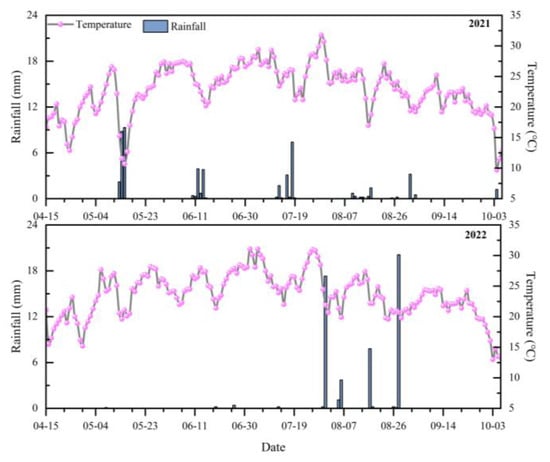
Figure 1.
Rainfall and average daily temperature during the experimental period in 2021 and 2022.

Table 1.
Soils’ physical and chemical properties before sowing.
Drip irrigation was used during the experiment, with the simultaneous irrigation of jujube and alfalfa, which was applied three times throughout the year: in the spring before sowing, after mowing the first crop, and in the winter after harvest. Supplemental irrigation was applied by using a hydrant pipe system in the experimental areas, and it was powered by electricity from the state grid. The nitrogen fertilizer used was urea (N: 46%); 50% of N was applied before sowing (12 April 2021 and 15 April 2022) and the remaining 50% was applied after the first harvest (4 July 2021 and 6 July 2022). N fertilizer was applied with irrigation water, and the annual irrigation volume was 4300 m3 hm−2. The alfalfa was harvested by hand, and artificial weeding was carried out during the crop growth period. At the same time, the redundant buds of the jujube trees were treated. The other management practices that were used were the same as those in the field.
2.2. Experimental Design
A two-factor split zone design was used, with the main zones for planting density (Figure 2)being D1 (210 kg ha−1 sowing rate; six rows), D2 (280 kg ha−1 sowing rate; eight rows), and D3 (350 kg ha−1 sowing rate; ten rows), and sub-zones for nitrogen levels of N0 (0 kg ha−1), N1 (80 kg ha−1), N2 (160 kg ha−1), and N3 (240 kg ha−1), with three replications and a randomized arrangement of blocks. Alfalfa was planted with a 0.5 m spacing from the trees, and the area of each plot was 42 m2 (length 14 m × width 3 m).
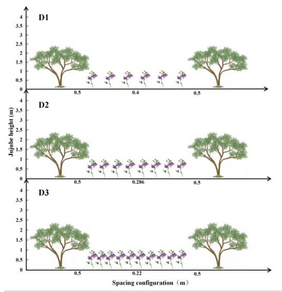
Figure 2.
Schematic diagram for the different planting densities of alfalfa.
2.3. Measurements and Calculations
2.3.1. Gas Sampling
The sampling of gas took place in 2022. Gas samples were collected using a static box, which consisted of a rectangular stainless steel base frame (30 × 15 × 10 cm3, L × W × H) with a removable lid box, which was fitted with a thermometer and fixed in 10 cm of soil in each plot, installed in the alfalfa rows. When the gas samples were collected, the lid was fastened to a groove in the base, and the groove was filled with water to form an enclosed sampling space during sampling. There were no weeds or crops inside the box. The gas samples were collected through a tee using a strictly numbered 100 mL medical syringe. A 5 cm ground thermometer was placed within 10 cm of each static box. The sampling frequency was 10 days. Four gas samples were collected within 30 min (0, 10, 20, and 30 min) between 11:00 and 13:00, and transferred to 300 mL aluminum foil gas collection bags using a syringe. At the time of sampling, the thermometer on the box was read, as well as the 5 cm ground thermometer. At the time of sampling, the soil moisture content was measured using a TDR-350 (SPECTRUM, Stamford, CT, USA) soil moisture thermometer.
2.3.2. Analysis of the Gas Samples
The collected gas samples were brought back to the laboratory and analyzed within 48 h. Specific parameters were analyzed using a gas chromatograph (model PANNA A91 plus) fitted with ECD and FID detectors. The equilibrium gas was high-purity N2. The ECD detector measured N2O at 300 °C with a tail blow flow rate of 5.0 mL min−1. The FID detector measured CO2 at 200 °C with a hydrogen flow rate of 40 mL min−1 and an air flow rate of 400 mL min−1. The gas samples were automatically separated within the column, and the concentrations of CO2, N2O, and CH4 in the gas samples were calculated from the slope of the linear regression between concentration and time. The physical meaning of the gas fluxes is that they represent the change in the mass of greenhouse gas per unit area of the observation box per unit time.
The calculation of GHGs gas fluxes was carried out using Equation (1) [25]:
where F indicates the GHGs emission fluxes, in mg m−2 h−1; ρ is the density of the measured gas under standard conditions, in kg m−3; T is the average temperature inside the airtight box during the sampling process, in °C; h is the height of the sampling box; dc/dt is the rate of change of the GHGs concentration inside the airtight box during the sampling process; and 273 is the constant of the gas equation.
The calculation of cumulative GHGs emissions was carried out using Equation (2) [26]:
where CE refers to the cumulative GHGs emissions, mg m−2; n is the total number of measurements during the cumulative emission observation time; i denotes the ith sampling; F refers to the emission fluxes of GHGs, in mg m−2 h−1; ti+1 − ti denotes the number of days between two adjacent measurement dates, in days.
The global warming potential was calculated using Equation (3) [5]:
where GWP is the global warming potential, in kg ha−1, which is a measure of the net greenhouse effect of agricultural land. On the 100 a scale, the warming potential per unit mass of CH4 and N2O is 26 and 256 times that of CO2, respectively. FCH4, FN2O, and FCO2 represent the CE of CH4, N2O, and CO2, respectively, for the entire measurement period, mg m−2.
To evaluate the emission reduction effect of soil carbon sequestration, the GHGs’ emission intensity was calculated using Equation (4) [27]:
2.3.3. Soil Physicochemical Properties
After the second crop of alfalfa was harvested, five points were randomly selected from each treatment plot, and soil samples were taken from the 0~10 cm soil layer by soil auger, naturally air-dried, and sieved (2 mm) for the determination of soil physicochemical properties. The indicators and methods were as follows: soil total nitrogen (TN)—soil total nitrogen was determined using the Kjeldahl method; soil available nitrogen (AN)—determined by the alkaline dissolution diffusion method; organic matter/organic carbon (SOM/SOC)—determined by external heating with potassium dichromate [28]; soil pH—determined using a soil pH meter (FE28); and soil bulk density (SBD)—determined by the ring knife method. The field water capacity and wilting point were determined with reference to the forest soil moisture’s physical properties (Standard LY/T1217-1999) [29].
2.3.4. Determination of the Yield and Its Fresh–Dry Ratio
Two crops of alfalfa were mowed in the experimental plots in one year, and the mowing was carried out when the alfalfa was in the early flowering stage. The first crop of 2021 was mowed on 3 July and the second crop on 12 October, while the first crop of 2022 was mowed on 5 July and the second crop was mown on 15 October. During alfalfa mowing, 1 × 1 m2 sample plots were set up, with a stubble height of 5 cm. All plant samples were subjected to 105 °C for 30 min to kill plant enzymes, then dried at 80 °C to a constant weight, and the fresh–dry ratio was calculated according to the ratio of the measured fresh and dry weights of the hay.
2.4. Statistical Analysis
Excel 2021 was chosen to organize the raw data and plot the tables. A two-factor split area analysis of the data was performed in DPS 9.01, and the statistical significance of the data at the p < 0.05 level was tested using the one-way least significant difference (LSD) method with the help of SPSS 26.0 software (SPSS Inc., Chicago, IL, USA). Origin 2021 (Origin Lab Corporation, Inc. Northampton, Northampton, MA, USA) was used for graphing.
3. Results
3.1. Effect of Planting Density and Nitrogen Application on Soil GHGs Emission Fluxes
The CO2 fluxes in alfalfa were in a state of emission throughout the year, which manifested as a carbon source. The CO2 fluxes under different densities and nitrogen fertilizer treatments showed a “single peak curve”, with the peak occurring in the first half of July, after irrigation and fertilization, and N3 > N2 > N1 > N0 under different density levels (Figure 3). In terms of the planting density, D1 had the highest annual average CO2 fluxes, which were 30.02% and 18.96% higher than that of D2 and D3, respectively. In terms of the nitrogen level, N3 significantly increased the CO2 fluxes from mid-June to late August under D2 and D3 levels. Different planting densities and nitrogen applications had significant effects on the CO2 fluxes in alfalfa, with reciprocal effects (p < 0.05). The differences in CO2 fluxes among treatments were not significant after September, when the temperature decreased.
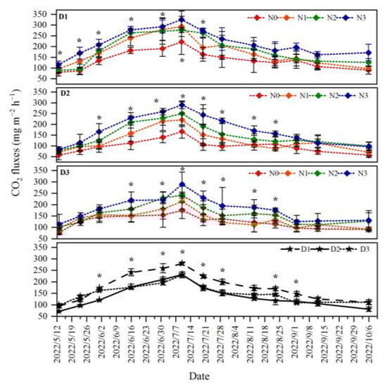
Figure 3.
Seasonal variation in CO2 carbon fluxes during the growing season of alfalfa. Note: * indicates that there are significant differences between different treatments, p < 0.05.
The N2O fluxes in alfalfa were emitted throughout the year and were a source of N2O, generally showing a “bimodal” zigzag fluctuation trend (Figure 4). When alfalfa entered the greening stage, the first peak in N2O fluxes appeared (around 23 May), and the second peak appeared in July (after irrigation and fertilization). Under the influence of the planting density factor, the trend of change was basically the same for all treatments, with D3 showing the highest emissions at the second peak, 24.55% and 29.82% higher than those of D1 and D2, respectively. In terms of the nitrogen level, N3 had the highest emissions at all planting densities, and the D3N3 flux emission of 0.24 mg m−2 h−1 increased by 22.44%, 51.89%, and 62.96% compared to N2, N1, and N0, respectively. Over time, the applied N fertilizer was gradually used up, and there was no significant difference in N2O emissions among treatments in the absence of exogenous N application.
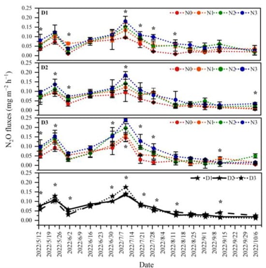
Figure 4.
Seasonal variation in N2O fluxes during the growing season of alfalfa. Note: * indicates that there are significant differences between different treatments, p < 0.05.
The results of the field monitoring showed that the overall CH4 uptake was in the range from −0.33 to 0.072 mg m−2 h−1, with a double peak in the growing season, showing a trend of high uptake in spring and summer and low uptake in fall (Figure 5). Meanwhile, the CH4 fluxes in the other periods of observation were basically in the vicinity of 0, with little fluctuation. The CH4 and N2O emission trends were mirror images of one another. There was a small peak in uptake on June 1, and the maximum CH4 flux uptake occurred around 11 July. That is, a week after irrigation, the CO2 emissions also peaked at this time, with the maximum uptake in the D2N0 treatment reaching 0.33 mg m−2 h−1, which was maintained for a relatively short period of time. Throughout the growing season, there was no significant difference between the treatments in terms of planting density; in terms of the nitrogen level, the uptake of each treatment was N0 > N1 > N2 > N3, in descending order. After August, the uptake of each treatment weakened, and there were treatments that began to show emissions, mainly N2 and N3, where excessive nitrogen application induced CH4 emissions.
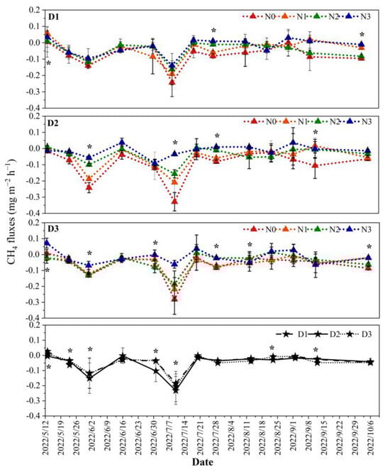
Figure 5.
Seasonal variation in CH4 fluxes during the growing season of alfalfa. Note: * indicates that there are significant differences between different treatments, p < 0.05.
3.2. Effects of Planting Density and Nitrogen Application on the GHGs’ Cumulative Emissions and Global Warming Trends in the Alfalfa Field
The differences in the cumulative soil GHG emissions and global warming trends under different planting densities and nitrogen applications are shown in Table 2. The effects of planting density, nitrogen application, and interactions between the two on the cumulative soil GHG emissions and GWP were not the same. Under the main factor of D1, the CO2 CE of the N3 treatment during the observation period amounted to 700.53 g m−2, which was 12.56%, 19.16%, and 50.91% higher than that of the N2, N1, and N0 treatments, respectively. The cumulative CH4 uptake in the D2 treatment was 45.80% and 19.70% more compared to the D1 and D3 treatments, respectively. The lowest cumulative N2O emissions during the observation period were only 137.11 mg m−2, emitted by the D1N0 treatment. The factor of nitrogen application had a highly significant effect on N2O CE, and the application of nitrogen fertilizers significantly increased the cumulative GHGs emissions, as well as the GWP, as compared to the treatment without nitrogen fertilizers. The nitrogen application factor had a highly significant effect on CH4 CE. Both increased nitrogen fertilizer application and irrational planting density increased the GWP, suggesting that both nitrogen application and density are major drivers of the GWP (p < 0.01). The GWP varied from 3597.60 to 7654.21 kg ha−1 during the observation period, and the GWP showed an increasing trend with the increase in nitrogen fertilizer application. Compared to the control treatment N0, the applied nitrogen fertilizer treatments increased the GWP to different degrees, and the N3 treatment was significantly higher than the other treatments. The GHG emission GHGI was used to visually assess the combined benefits of GHGI and yield, with smaller GHGI values implying a smaller global warming effect from the same crop yield. GHGI varied from 0.061 to 0.106 kg CO2-eq kg−1. Optimizing planting density and nitrogen application (D2N2) significantly offsets the negative environmental impact and reduces the alfalfa GHGI values.
Table 2.
Effects of planting density and nitrogen application on the cumulative soil GHG emissions and global warming potential.
3.3. Effect of Planting Density and Nitrogen Application on Soil Hydrothermal Properties
During the observation period, the 0–5 cm soil temperature and soil moisture content were monitored simultaneously, and it was found that the seasonal change in soil temperature in each treatment had a trend of “high in summer and fall, and low in spring and winter” (Figure 6). Seasonal changes in soil temperature showed a trend of first rising and then falling. In early May, as alfalfa began to regreen, the soil temperature showed a wave-like gradual increase. Following the first alfalfa harvest in early July, which reduced the vegetation cover, the soil temperature rose rapidly, reaching a maximum in mid-July with an average temperature of 27.65 °C. By mid-September, the soil temperatures all decreased to the lowest values observed during the period, with the lowest for D3N3, at 12.75 °C.
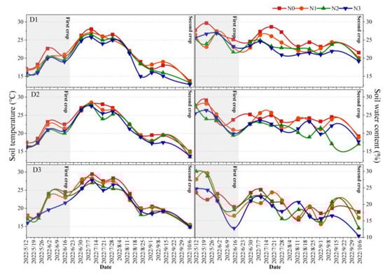
Figure 6.
Effect of planting density and nitrogen application on soil temperature and water content.
Soil moisture is generally high in spring and summer and low in fall and winter, showing a “double peak” phenomenon. The first peak was caused by spring irrigation, and the second peak was caused by irrigation after the first mowing. During the experimental period, the field water capacity was 28.53% and the wilting point was 11.49%. This decreased to the lowest value of the first crop in mid-June, with an average value of 20.33%. Irrigation after mowing on 6 July resulted in a gradual increase in the soil surface moisture content and reached a maximum for the second crop in mid-July, when the surface soil moisture content was approximately 28.6%. Subsequently, the soil surface water content gradually decreased and stabilized at approximately 10~25%.
3.4. Effect of Planting Density and Nitrogen Application on Soils’ Physical and Chemical Properties
Different planting densities and nitrogen applications had significant effects on the soils’ physicochemical properties (Table 3). There were differences in the effects of nitrogen application treatments on the physicochemical properties of the surface soil (10 cm) of alfalfa at different planting densities, and the nitrogen application treatments N3 and N2 significantly reduced the pH value of the soil. The decreases that occurred under the D1 factor compared to the no-nitrogen-fertilizer treatment N0 were 2.79% and 1.01% for the N3 and N2 treatments, respectively. Analysis of variance (ANOVA) revealed that the D2N2 treatment had the highest content of TN, quick nitrogen, at 2.34 g kg−1 and 48.67 mg kg−1, respectively, with an increase of 188.88% and 163.08%, compared to the D1N0 treatment with the lowest content. Multifactorial ANOVA showed that nitrogen application factors had highly significant (p < 0.01) effects on TN and significant (p < 0.05) effects on quick nitrogen. Under the combined effects of the different treatments, the alfalfa soil organic carbon and organic matter showed different differences, and under the D2 factor, there were significant differences between the SOC and SOM treatments. Additionally, the N2 treatment had the highest content, which was 14.14 g kg−1 and 8.20 g kg−1, respectively. Nitrogen application factors had a highly significant effect on SOM and SOC (p < 0.01). D2N2 had the smallest bulk density of 1.11 g cm−3. The better the soil structure and aeration, the more favorable it was for plant growth.
Table 3.
Effect of planting density and nitrogen application on soils’ physicochemical properties.
3.5. Effect of Planting Density and Nitrogen Application on the Yield and Fresh–Dry Ratio of Alfalfa
As can be seen in Figure 7, it was found that the alfalfa yield in 2022 was higher than the alfalfa yield in 2021, with an average increase of up to 52.18%. Consistently, it was found that the head crop yield was higher than the yield of the second crop, and that the fresh–dry ratio had an inverse relationship with the yield. The yield increased with increasing density and there was no significant difference between the fresh–dry ratios at different densities. The yield decreased with decreasing nitrogen application, the fresh–dry ratio decreased and then increased with increasing nitrogen application, and excessive nitrogen application increased the fresh–dry ratio of alfalfa. The highest yield was obtained from the first crop of the D3N3 treatment in 2021, when the fresh–dry ratio was the lowest at 13.32%. A highly significant difference (p < 0.01) was consistently obtained in the yield among the different nitrogen application treatments under the D3 main factor, and a significant difference (p < 0.05) was obtained among the different nitrogen application treatments under the D2 main factor in 2022. The highest yield of 43,366.67 kg ha−1 was recorded in the first crop of D2N2 in 2022, which was 52.34% higher compared to the no-fertilization-treatment D2N0. Moreover, it was concluded from the line graph that the N2 treatment maintained the lowest fresh–dry ratio among the N application treatments under different density factors, fluctuating in the range from 22.46% to 26.11%.
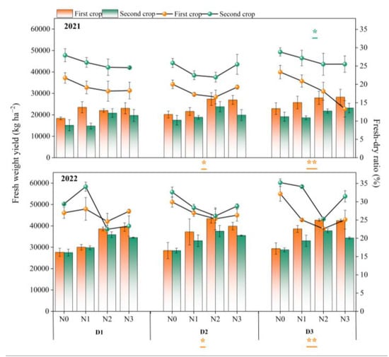
Figure 7.
Effect of planting density and nitrogen application on the yield and fresh–dry ratio of alfalfa. Note: The line graphs represent the fresh–dry ratios of the different treatments, while the bar graphs represent the fresh grass yields of the different treatments, * indicates significant differences between different treatments, p < 0.05, ** indicates the extremely significant difference between different treatments, p < 0.01.
3.6. Related Analysis
In order to further clarify the relationship between the GHGs and soil indicators, (Figure 8), among the environmental factors in this study, ST had a strong influence on GHG emissions, with significant positive correlations with CO2 fluxes and the GWP (p < 0.05). Highly significant positive correlations were also found for N2O and CH4 fluxes (p < 0.01), i.e., ST is an influencing factor that is sensitive to soil carbon fluxes. In contrast, SWC resulted in the opposite conclusion to ST, and there was a highly significant negative correlation (p < 0.01) between soil hydrothermal properties, with soil respiration responding more strongly to ST than SWC. Meanwhile, there was a highly significant positive correlation (p < 0.01) between yield and a number of metrics, including TN, AN, SOC, ST, CO2 fluxes, N2O fluxes, CH4 fluxes, CO2 CE, N2O CE, CH4 CE, and GWP. Conversely there was a highly significant negative correlation (p < 0.01) between yield and alfalfa FDR. The seven GHG indicators—CO2 fluxes, N2O fluxes, CH4 fluxes, CO2 CE, N2O CE, CH4 CE, and GWP—showed highly significant positive correlations with one another (p < 0.01). The correlation coefficient between the GWP and CO2 CE metrics reached 1, indicating a perfect positive correlation. GHGI had a highly significant positive correlation with the GWP (p < 0.01), but a negative but non-significant correlation with yield, while the GWP can be used to explain changes in GHGI alone. Among the soil factors, TN had a positive correlation with the GHGs indicators as well as the soil physicochemical property indicators AN, SOM, and SOC. There was no significant correlation between SBD and the indicators in this study, and the correlation coefficients were all less than 0.22.
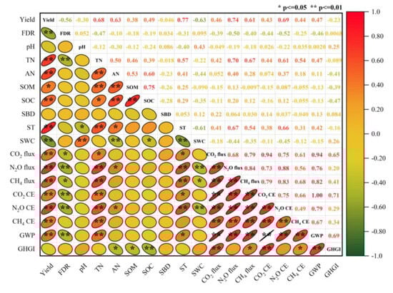
Figure 8.
Correlation analysis of the GHG emission indicators with the soil physicochemical properties and alfalfa yield. Note: The abbreviations in the table indicate the following: FDR, fresh–dry ratio; TN, total soil nitrogen; AN, quick-acting soil nitrogen; SOM, soil organic matter; SOC, soil organic carbon; SBD, soil bulk density; ST, soil temperature; SWC, soil water content; CO2 CE, cumulative CO2 emissions; N2O CE, cumulative N2O emissions; CH4 CE, cumulative CH4 emissions; GWP, global warming potential; GHGI, greenhouse gas emission intensity.
4. Discussion
Global climate change is a major challenge that humanity is currently facing, and agriculture plays an important role in global anthropogenic GHG emissions [30]. Therefore, an important way to reduce soil GHG emissions is to adopt advanced crop production techniques. It has been shown that intercropping can more effectively reduce soil CO2 emissions than monocropping [31]. In this study, alfalfa soil respiration peaked in the peak growth stage (July) (Figure 3 and Figure 4), which may be related to soil temperature (ST). Meanwhile, a higher ST promoted alfalfa root respiration and increased microbial activity, which, in turn, increased the soil respiration intensity. The model of increasing density and reducing nitrogen has been proven to be beneficial for GHG emission reduction: on the one hand, it reduces the amount of nitrogen applied, which indirectly reduces the carbon emissions of nitrogen fertilizer in various links, such as production, transportation, and storage; on the other hand, it directly reduces CH4 and N2O emissions [32]. This experimental study showed that GHGs fluxes exhibited lower emissions at the D2 density level (Figure 3, Figure 4 and Figure 5), indicating that appropriately increasing the alfalfa density is beneficial to reducing GHGs emissions in the jujube–alfalfa intercropping system. The CH4 emissions of the jujube–alfalfa intercropping system varied from −0.33 to 0.072 mg m−2 h−1, and the appropriate alfalfa density exerted a certain deposition effect on the atmospheric CH4 uptake, which was similar to the results of the study on rice by Zhu Xiangcheng et al. [32]. A large number of studies have shown that excessive nitrogen fertilizer inputs are the main factors contributing to GHG emissions from agricultural fields [13,33], and methods for optimizing the nitrogen inputs in cropping systems have become a primary issue in reducing GHs emissions from fields [34]. Nitrogen fertilizer application safeguards individual crop development, while planting density is an effective measure for coordinating individual crops and populations, with significant interactions between nitrogen fertilizer and density treatments. The most direct practice to achieve the nitrogen management goal is to reduce the application of nitrogen fertilizer on farmland, because N2O emissions from farmland are positively correlated with the nitrogen input of the cropping system [35]. In this study, the trends of carbon flux dynamics for N2O and CH4 during the observation period were opposing “peaks” and “valleys”, forming “mirror images” of one another. The jujube–alfalfa intercropping system as a whole showed a “sink” of CH4, and N3 increased the average emission fluxes of NO2, CO2, and CH4 during the growing season of alfalfa compared to with N0, N1, and N2, which was attributed to a decrease in the activity of methanotrophic bacteria caused by an increase in nitrogen application [36], resulting in a decrease in CH4 uptake and an increase in emissions. The application of nitrogen was also the main driver of GWP. There is no conclusive evidence of the effect of planting density on GHGs emissions thus far. In this study, optimizing planting density and nitrogen application (D2N2) significantly offset the negative environmental impacts and reduced alfalfa GHGI by only 0.061 kg CO2-eq kg−1 (Table 2).
The ST increase in this study promoted CO2 and N2O fluxes and suppressed CH4 uptake, which is consistent with the findings of some previous studies [37,38]. Additionally, the correlation coefficient for soil GHG emissions exceeded 0.31, a finding that is consistent with the results of Ghani et al.’s study [27], but at variance with the conclusion of an exponential negative correlation between soil respiration and ground temperature drawn by Tsets gatu et al. [39]. The reason for this may be that proper warming promotes microorganism activity in the soil, accelerates the decomposition of organic matter and microbial activity in the soil, and thus increases the rate of GHG production and diffusion to the surface. In this study, soil GHGs showed a negative correlation with soil water content, similar to the results of Li [40]. This may be due to the fact that the hydrothermal coupling effect and the effect of ST on soil GHGs were significantly higher than that of SWC, and the effect of SWC on GHGs was masked by the effect of ST. This is because water molecules fill the voids in the soil when the soil water content is high, which hinders the diffusion of O2 and CO2, thus leading to a reduction in soil respiration [41]. Another reason may be that the complex boundary conditions of intercropping systems affect the variations in their soil water content.
In addition to the major abiotic drivers of soil moisture and temperature, soil GHG fluxes are directly regulated by biological factors, including root respiration, microbial activity, and soil nutrients [42]. The effects of soils’ physicochemical properties on soil GHG emissions are intricate. The alfalfa–rhizobium symbiotic nitrogen fixation system converts atmospheric nitrogen into mineral nitrogen for crop utilization during alfalfa growth and development [43]. Therefore, there is no need to incorporate excess nitrogen sources, and the application of excess nitrogen would only increase the burden of GHG emissions. The nitrogen application treatments reduced the pH while increasing the content of total and quick-acting nitrogen contents in the soil, and some studies have shown that long-term nitrogen application decreases the soil pH [44,45]. Additionally, the application of nitrogen fertilizers can reduce the leaching of quick-acting nutrients [46], promote the conversion of soluble substances, and enhance the content of quick-acting nutrients in soil (Table 3). The nitrogen application factor had a highly significant effect on TN, which may be due to the increase in the amount of nitrogen application increasing the effectiveness of nitrogen, resulting in greater N2O production. The effect of nitrogen application on GHG emissions is due to the effect of nitrogen fertilization on microbial development and soil respiration, both of which are dependent on soil organic matter [47]. This is why nitrogen application factors had highly significant effects on SOM and SOC (Table 3). In this study, it can be confirmed that the factors affecting soil GHG emissions were numerous and intricate, so an analysis of the dynamics of soil respiration needs to take into account the individual or combined effects of as many of these factors as possible.
Increasing planting density, which can improve the utilization of natural resources, is a key step for achieving high yields and can increase the amount of alfalfa fresh grass (Figure 8). There was no significant pattern of differences in GHGs emissions based on planting density (Figure 4, Figure 5 and Figure 6), indicating that planting density is not a major limiting factor for GHG emissions. Similarly to Meng et al. [48], this study found that medium density (D2) is not favorable for alfalfa yield. The fresh–dry ratio of alfalfa, which is the expression of dry matter accumulation and the definition of utilization value, was negatively correlated with alfalfa quality. The excessive application of nitrogen led to an increase in the fresh–dry ratio (Figure 7), which is similar to the findings of Li et al. [49], who found that a moderate amount of nitrogen fertilizer will have a negative effect on the fresh–dry ratio of alfalfa, while a small or excessive amount has a positive effect.
The planting density and nitrogen application in the jujube–alfalfa intercropping system in this study may not be conducive to the optimization of alfalfa yield and GHG emission reductions in other areas, and the trial period was short. Therefore, further long-term comprehensive investigations are still needed to reduce the GHG emissions caused by irrational fertilization and tillage practices and to further mitigate GHG emissions from farmland.
5. Conclusions
In this study, the medium nitrogen level (N2) was more favorable for improving the alfalfa yield and resource use efficiency, resulting in low soil GHG emissions. The D2N2 (eight rows planted in one film; N = 160 kg ha−1) treatment was the best combination for alfalfa yield and GHG emissions, while simultaneously ensuring lower carbon emission intensity values, constituting a better soil structure, and resulting in the best soil physicochemical properties. In conclusion, considering the crop yield and GHG emissions, the selection of medium density and a medium nitrogen level (D2N2) for production in a jujube intercropping system is the most suitable, and can promote the sustainable development of crop production and the ecological environment.
Author Contributions
Conceptualization, G.C.; methodology, T.L.; software, T.L.; validation, G.C.; formal analysis, G.C.; investigation, T.L.; resources, Z.F.; data curation, Y.Z.; writing—original draft preparation, T.L.; writing—review and editing, Z.C. and J.W.; visualization, S.W.; supervision, G.C.; project administration, S.W.; funding acquisition, Y.Z. All authors have read and agreed to the published version of the manuscript.
Funding
This research was funded by the National Natural Science Foundation of China (32060449), the National Key Research and Development Program of China (2016YFC0501400), the graduate student innovation project of Xinjiang Corps in 2023 (Effects of nitrogen fertilizer reduction and crop rotation on carbon and nitrogen footprints of agro-fruit composite systems) and the Graduate Student Innovation Program of Tarim University (TDGRI202215).
Data Availability Statement
The entire set of raw data presented in this study is available upon request from the corresponding author.
Conflicts of Interest
The authors declare no conflicts of interest.
References
- Shakoor, A.; Shahbaz, M.; Farooq, T.H.; Sahar, N.E.; Shahzad, S.M.; Altaf, M.M.; Ashraf, M. A global meta-analysis of greenhouse gases emission and crop yield under no-tillage as compared to conventional tillage. Sci. Total. Environ. 2021, 750, 142299. [Google Scholar] [CrossRef]
- Kan, Z.R.; Liu, W.X.; Liu, W.S.; Lal, R.; Dang, Y.P.; Zhao, X.; Zhang, H.L. Mechanisms of soil organic carbon stability and its response to no-till: A global synthesis and perspective. Glob. Chang. Biol. 2022, 28, 693–710. [Google Scholar] [CrossRef]
- Malhi, S.S.; Zentner, R.P.; Heier, K. Effectiveness of alfalfa in reducing fertilizer N input for optimum forage yield, protein concentration, returns and energy performance of bromegrass-alfalfa mixtures. Nutr. Cycl. Agroecosyst. 2002, 62, 219–227. [Google Scholar] [CrossRef]
- Li, C.; Xiong, Y.; Huang, Q.; Xu, X.; Huang, G. Impact of irrigation and fertilization regimes on greenhouse gas emissions from soil of mulching cultivated maize (Zea mays L.) field in the upper reaches of Yellow River, China. J. Clean. Prod. 2020, 259, 120873. [Google Scholar] [CrossRef]
- IPCC. Contribution of Working Groups I, II and III to the Fifth Assessment Report of the Intergovernmental Panel on Climate Change; Cambridge University Press: Cambridge, UK, 2014. [Google Scholar]
- Vermeulen, S.J.; Campbell, B.M.; Ingram, J.S.I. Climate change and food systems. Annu. Rev. Environ. Resour. Econ. 2012, 37, 195–222. [Google Scholar] [CrossRef]
- Smith, P.; Martino, D.; Cai, Z.; Gwary, D.; Janzen, H.; Kumar, P.; Bruce, M.C.; Stephen, O.; Frank, O.; Charles, R.; et al. Greenhouse gas mitigation in agriculture. Philos. Trans. R. Soc. B 2008, 363, 789–813. [Google Scholar] [CrossRef] [PubMed]
- Xu, C.; Huang, S.; Tian, B.; Ren, J.; Meng, Q.; Wang, P. Manipulating planting density and nitrogen fertilizer application to improve yield and reduce environmental impact in Chinese maize production. Front. Plant. Sci. 2017, 8, 1234. [Google Scholar] [CrossRef] [PubMed]
- Chen, W.; Wang, Y.; Zhao, Z.; Cui, F.; Gu, J.; Zheng, X. The effect of planting density on carbon dioxide, methane and nitrous oxide emissions from a cold paddy field in the Sanjiang Plain, northeast China. Agric. Ecosyst. Environ. 2013, 178, 64–70. [Google Scholar] [CrossRef]
- Yang, T.; Li, F.; Zhou, X.; Xu, C.; Feng, J.; Fang, F. Impact of nitrogen fertilizer, greenhouse, and crop species on yield-scaled nitrous oxide emission from vegetable crops: A meta-analysis. Ecol. Indic. 2019, 105, 717–726. [Google Scholar] [CrossRef]
- He, H.; Hu, Q.; Pan, F.; Pan, X. Evaluating Nitrogen Management Practices for Greenhouse Gas Emission Reduction in a Maize Farmland in the North China Plain: Adapting to Climate Change. Plants 2023, 12, 3749. [Google Scholar] [CrossRef]
- IPCC. Climate Change 2021: The Physical Science Basis. In Contribution of Working Group I to the Sixth Assessment Report of the Intergovernmental Panel on Climate; Agenda: Newcastle upon Tyne, UK, 2021. [Google Scholar]
- Wang, X.; Chen, Y.; Chen, X.; He, R.; Guan, Y.; Gu, Y.; Chen, Y. Crop production pushes up greenhouse gases emissions in China: Evidence from carbon footprint analysis based on national statistics data. Sustainability 2019, 11, 4931. [Google Scholar] [CrossRef]
- Abagandura, G.O.; Sekaran, U.; Singh, S.; Singh, J.; Ibrahim, M.A.; Subramanian, S.; Owens, V.N.; Kumar, S. Intercropping kura clover with prairie cordgrass mitigates soil greenhouse gas fluxes. Sci. Rep. 2020, 10, 7334. [Google Scholar] [CrossRef] [PubMed]
- Jiang, J.; Jiang, S.; Xu, J.; Wang, J.; Li, Z.; Wu, J.; Zhang, J. Lowering nitrogen inputs and optimizing fertilizer types can reduce direct and indirect greenhouse gas emissions from rice-wheat rotation systems. Eur. J. Soil Biol. 2020, 97, 103152. [Google Scholar] [CrossRef]
- Solanki, M.K.; Wang, F.; Wang, Z.; Li, C.; Lan, T.; Singh, R.K.; Singh, P.; Yang, L.; Li, Y. Rhizospheric and endospheric diazotrophs mediated soil fertility intensification in sugarcane-legume intercropping systems. J. Soils Sediments 2019, 19, 1911–1927. [Google Scholar] [CrossRef]
- Layek, J.; Das, A.; Mitran, T.; Nath, C.; Meena, R.S.; Yadav, G.S.; Shivakumar, B.G.; Kumar, S.; Lal, R. Cereal+ legume intercropping: An option for improving productivity and sustaining soil health. In Legumes for Soil Health and Sustainable Management; Springer: Singapore, 2018; pp. 347–386. [Google Scholar]
- Gao, J.S.; Cao, W.D.; Li, D.C.; Xu, M.; Zeng, X.; Me, J.; Zhang, W. Effects of long-term double-rice and green manure rotation on rice yield and soil organic matter in paddy field. Shengtai Xuebao/Acta Ecol. Sin. 2011, 31, 4542–4548. [Google Scholar]
- Sainju, U.M.; Caesar-TonThat, T.; Lenssen, A.W.; Barsotti, J.L. Dryland soil greenhouse gas emissions affected by cropping sequence and nitrogen fertilization. Soil. Sci. Soc. Am. J. 2012, 76, 1741–1757. [Google Scholar] [CrossRef]
- Meng, Y.Q.; Liu, Y.F.; Wan, S.M.; Zhou, T.T.; Li, Y.F.; Wang, P.J.; Tian, Y.G.; Chen, G.D. Effects of Distance from Tree Line on Soil Physicochemical Properties Along with Alfalfa Yield in jujube–alfalfa Intercropping System. J. Tarim Univ. 2020, 32, 24–30. [Google Scholar]
- Yin, W.; Chai, Q.; Guo, Y.; Feng, F.; Zhao, C.; Yu, A.; Liu, C.; Fan, Z.; Hu, F.; Chen, G. Reducing carbon emissions and enhancing crop productivity through strip intercropping with improved agricultural practices in an arid area. J. Clean. Prod. 2017, 166, 197–208. [Google Scholar] [CrossRef]
- Chapagain, T.; Pudasaini, R.; Ghimire, B.; Gurung, K.; Choi, K.; Rai, L.; Magar, S.; Bishnu, B.K.; Raizada, M.N. Intercropping of maize, millet, mustard, wheat and ginger increased land productivity and potential economic returns for smallholder terrace farmers in Nepal. Field Crop. Res. 2018, 227, 91–101. [Google Scholar] [CrossRef]
- Fan, W.X.; Li, T.T.; Chen, G.D.; Mao, T.Y.; Hu, Q.; Zhai, Y.L.; Wan, S.M. Effects of spacing on soil aggregate organic carbon, total nitrogen and yield of alfalfa intercropped with jujube. Soil Fertil. Sci. China 2023, 8, 67–75. [Google Scholar]
- Fan, W.X.; Wang, M.G.; Chen, G.D.; Li, T.T.; Lin, F.; Zhai, Y.L.; Wu, Q.Z.; Wan, S.M. Effect of a jujube–alfalfa intercropping system on soil chemical properties and microorganisms in the oasis irrigation area of southern Xinjiang. Pratacult. Sci. 2022, 39, 39–47. [Google Scholar]
- Rolston, D.E. Gas flux. In Methods of Soil Analysis Part 1. Agronomy Monograph 9, 2nd ed.; Klute, A., Ed.; ASA and SSSA: Madison, WI, USA, 1986; pp. 1103–1119. [Google Scholar]
- Afreh, D.; Zhang, J.; Guan, D.; Liu, K.; Song, Z.; Zheng, C.; Deng, A.; Feng, X.; Zhang, X.; Wu, Y.; et al. Long-term fertilization on nitrogen use efficiency and greenhouse gas emissions in a double maize cropping system in subtropical China. Soil Tillage Res. 2018, 180, 259–267. [Google Scholar] [CrossRef]
- Ghani, M.U.; Kamran, M.; Ahmad, I.; Arshad, A.; Zhang, C.; Zhu, W.; Shanning, L.; Hou, F. Alfalfa-grass mixtures reduce greenhouse gas emissions and net global warming potential while maintaining yield advantages over monocultures. Sci. Total Environ. 2022, 849, 157765. [Google Scholar] [CrossRef] [PubMed]
- Bao, S.D. Soil Agrochemical Analysis; China Agricultural Press: Beijing, China, 2000. [Google Scholar]
- LY/T1217-1999; Forestry Industry Standard of the People’s Republic of China-Determination of forest soll permanent wilting water content. China Forestry Administration: Beijing, China, 1999.
- Gan, Y.; Liang, C.; Wang, X.; McConkey, B. Lowering carbon footprint of durum wheat by diversifying cropping systems. Field Crop. Res. 2011, 122, 199–206. [Google Scholar] [CrossRef]
- Yin, W.; Feng, F.; Zhao, C.; Yu, A.; Hu, F.; Chai, Q.; GAN, Y.T.; Guo, Y. Integrated double mulching practices optimizes soil temperature and improves soil water utilization in arid environments. Int. J. Biometeopol. 2016, 60, 1423–1437. [Google Scholar] [CrossRef] [PubMed]
- Zhu, X.G.; Zhang, Z.P.; Zhang, J.; Deng, A.X.; Zhang, W.J. Effects of increased planting density with reduced nitrogen fertilizer application on rice yield, N use efficiency and greenhouse gas emission in Northeast China. Chin. J. Appl. Ecol. 2016, 27, 453–461. [Google Scholar]
- Daly, E.J.; Hernandez-Ramirez, G. Sources and priming of soil N2O and CO2 production: Nitrogen and simulated exudate additions. Soil Biol. Biochem. 2020, 149, 107942. [Google Scholar] [CrossRef]
- Wang, X.; Chen, Y.; Yang, K.; Duan, F.; Liu, P.; Wang, Z.; Wang, J. Effects of legume intercropping and nitrogen input on net greenhouse gas balances, intensity, carbon footprint and crop productivity in sweet maize cropland in South China. J. Clean. Prod. 2021, 314, 127997. [Google Scholar] [CrossRef]
- Fan, Y.; Hao, X.; Carswell, A.; Misselbrook, T.; Ding, R.; Li, S.; Kang, S. Inorganic nitrogen fertilizer and high N application rate promote N2O emission and suppress CH4 uptake in a rotational vegetable system. Soil Till. Res. 2021, 206, 104848. [Google Scholar] [CrossRef]
- Sainju, U.M.; Stevens, W.B.; Caesar-TonThat, T.; Liebig, M.A. Soil greenhouse gas emissions affected by irrigation, tillage, crop rotation, and nitrogen fertilization. J. Environ. Qual. 2012, 41, 1774–1786. [Google Scholar] [CrossRef]
- Singh, B.K.; Bardgett, R.D.; Smith, P.; Reay, D.S. Microorganisms and climate change: Terrestrial feedbacks and mitigation options. Nat. Rev. Microbiol. 2010, 8, 779–790. [Google Scholar] [CrossRef] [PubMed]
- Butterbach-Bahl, K.; Baggs, E.M.; Dannenmann, M.; Kiese, R.; Zechmeister-Boltenstern, S. Nitrous oxide emissions from soils: How well do we understand the processes and their controls? Philos. Trans. R. Soc. B 2013, 368, 20130122. [Google Scholar] [CrossRef] [PubMed]
- Tao, G.T.; Zhao, J.; Sun, Q.Z.; Zhu, Y.H.; Zhao, S.F. Effect of Differ ent Herbages on Soil Respir ation in Agropastor al Region. J. Agro-Environ. Sci. 2006, 06, 1513–1517. [Google Scholar]
- Li, H.S.; Liu, G.Q.; Wang, H.Z.; Li, W.H.; Chen, C.G. Seasonal changes in soil respiration and the driving factors of four woody plant communities in the Loess Plateau. Acta Ecol. Sin. 2008, 29, 4099–4106. [Google Scholar]
- Lin, Z.; Zhang, R.; Tang, J.; Zhang, J. Effects of high soil water content and temperature on soil respiration. Soil Sci. 2011, 176, 150–155. [Google Scholar] [CrossRef]
- Kitzler, B.; Zechmeister-Boltenstern, S.; Holtermann, C.; Skiba, U.; Butterbach-Bahl, K. Nitrogen oxides emission from two beech forests subjected to different nitrogen loads. Biogeosciences 2006, 3, 293–310. [Google Scholar] [CrossRef]
- Zhang, M.X.; Zhao, L.Y.; He, Y.Y.; Hu, J.P.; Hu, G.W.; Zhu, Y.; Aziz, k.; Xiong, Y.C.; Zhang, J.L. Potential roles of iron nanomaterials in enhancing growth and nitrogen fixation and modulating rhizomicrobiome in alfalfa (Medicago sativa L.). Bioresour. Technol. 2024, 391, 129987. [Google Scholar] [CrossRef]
- Yang, Y.D.; Wang, Z.M.; Zeng, Z.H. Effects of Long-Term Different Fertilization and lrrigation Managements on Soil Bacterial Abundance, Diversity and Composition. Sci. Agric. Sin. 2018, 51, 290–301. [Google Scholar]
- Luo, P.Y.; Fan, Y.; Yang, J.F.; Ge, Y.F.; Cai, F.F.; Huan, X.R. Influence of long-term fertilization on abundance of ammonia oxidizing bacteria and archaea in brown soil. J. Plant Nutr. Fertil. 2017, 23, 678–685. [Google Scholar]
- Sardans, J.; Penuelas, J.; Estiarte, M.; Prieto, P. Warming and drought alter C and N concentration, allocation and accumulation in a Mediterranean shrubland. Glob. Chang. Biol. 2018, 14, 2304–2316. [Google Scholar] [CrossRef]
- Li, X.; Chen, S.; Yang, Z.; Lin, C.; Xiong, D.; Lin, W.; Xu, C.; Chen, G.; Xie, J.; Li, Y.; et al. Will heterotrophic soil respiration be more sensitive to warming than autotrophic respiration in subtropical forests? Eur. J. Soil. Sci. 2018, 70, 655–663. [Google Scholar] [CrossRef]
- Meng, K.; Li, X.Y.; Jia, Z.Y.; Jin, H.Q.; Mi, F.G. Effects of planting density on the growth, yield and nutritional quality of alfalfa in central Inner Mongolia. Acta Pratacult. Sin. 2019, 28, 73. [Google Scholar]
- Li, X.Y.; Xiao, Y.Z.; Meng, K.; Mi, F.G. The Effect of Fertilizing with Formula on stem leaf ratio and ratio of dry-and-wet weight of alfalfa. Grassl. Pratacult. 2015, 27, 32–39. [Google Scholar]
Disclaimer/Publisher’s Note: The statements, opinions and data contained in all publications are solely those of the individual author(s) and contributor(s) and not of MDPI and/or the editor(s). MDPI and/or the editor(s) disclaim responsibility for any injury to people or property resulting from any ideas, methods, instructions or products referred to in the content. |
© 2024 by the authors. Licensee MDPI, Basel, Switzerland. This article is an open access article distributed under the terms and conditions of the Creative Commons Attribution (CC BY) license (https://creativecommons.org/licenses/by/4.0/).