Article

Automated Seedling Contour Determination and Segmentation Using Support Vector Machine and Image Features

1
Department of Agricultural Machinery Engineering, Graduate School, Chungnam National University, Daejeon 34134, Republic of Korea
2
Department of Smart Agricultural Systems, Graduate School, Chungnam National University, Daejeon 34134, Republic of Korea
3
Jeonnam Agricultural Research and Extension Services, Naju 58213, Republic of Korea
4
Jeonbuk Regional Branch, Korea Electronics Technology Institute (KETI), Jeonju 54853, Republic of Korea
*
Author to whom correspondence should be addressed.
Agronomy 2024, 14(12), 2940; https://doi.org/10.3390/agronomy14122940
Submission received: 6 November 2024 / Revised: 30 November 2024 / Accepted: 7 December 2024 / Published: 10 December 2024

Abstract

:
Boundary contour determination during seedling image segmentation is critical for accurate object detection and morphological characterization in agricultural machine vision systems. The traditional manual annotation for segmentation is labor-intensive, time-consuming, and prone to errors, especially in controlled environments with complex backgrounds. These errors can affect the accuracy of detecting phenotypic traits, like shape, size, and width. To address these issues, this study introduced a method that integrated image features and a support vector machine (SVM) to improve boundary contour determination during segmentation, enabling real-time detection and monitoring. Seedling images (pepper, tomato, cucumber, and watermelon) were captured under various lighting conditions to enhance object–background differentiation. Histogram equalization and noise reduction filters (median and Gaussian) were applied to minimize the illumination effects. The peak signal-to-noise ratio (PSNR) and the structural similarity index measure (SSIM) were used to select the clip limit for histogram equalization. The images were analyzed across 18 different color spaces to extract the color features, and six texture features were derived using the gray-level co-occurrence matrix (GLCM) method. To reduce feature overlap, sequential feature selection (SFS) was applied, and the SVM was used for object segmentation. The SVM model achieved 73% segmentation accuracy without SFS and 98% with SFS. Segmentation accuracy for the different seedlings ranged from 81% to 98%, with a low boundary misclassification rate between 0.011 and 0.019. The correlation between the actual and segmented contour areas was strong, with an R2 up to 0.9887. The segmented boundary contour files were converted into annotation files to train a YOLOv8 model, which achieved a precision ranging from 96% to 98.5% and a recall ranging from 96% to 98%. This approach enhanced the segmentation accuracy, reduced manual annotation, and improved the agricultural monitoring systems for plant health management. The future direction involves integrating this system with advanced methods to address overlapping image segmentation challenges, further enhancing the real-time seedling monitoring and optimizing crop management and productivity.

1. Introduction

Seedling segmentation, the process of distinguishing seedlings from their background in images, plays a crucial role in precision agriculture, where the early and accurate detection of plant health issues is essential for optimizing crop production and resource use [1]. The production of seedlings, particularly in controlled environments, like plant factories and greenhouses, has increased due to the growing demand for efficient and sustainable farming practices [2,3]. These facilities offer significant advantages in managing plant growth conditions, including the lighting, temperature, humidity, and nutrient levels, all of which can be controlled with precision to ensure maximum yields and quality [4,5,6]. However, these controlled environments also introduce challenges, particularly in monitoring plants’ health condition, which is crucial for the early detection of stress symptoms, diseases, and other growth-limiting factors [7]. The traditional health monitoring methods, such as manual inspection, are often labor-intensive, subjective, and prone to errors. As a result, there is an increasing need for automated, real-time plant health monitoring systems that can operate on a large scale, without human intervention [8,9].
To address these issues, segmentation techniques integrated with boundary contour determination have emerged as an important tool for the automation of seedling health monitoring systems [10,11]. Segmentation with boundary contour determination enables the precise representation of seedling structures from their background in images, allowing for the accurate extraction of key features, such as plant height, leaf area, and color [12]. Boundary contour determination plays a vital role in refining the boundaries of segmented objects, ensuring that intricate details, such as fine stems and small leaves, are preserved [11]. This is especially important in plant health monitoring, where even slight changes in seedling morphology can signal the onset of stress or disease symptoms [13]. Furthermore, boundary contour determination facilitates the automatic generation of annotation files, significantly reducing the manual effort required to create large, annotated datasets for use in machine learning applications [14].
Computer vision has emerged as a transformative technology in agriculture, offering the ability to automatically monitor plants growth and health through image analysis [2]. It has become an essential tool for controlled horticulture systems such as plant factories, where every aspect of the environment is carefully regulated [15]. Unlike traditional open-field farming, where factors such as weather and soil conditions are largely uncontrollable, plant factories offer a highly structured place in which computer vision can achieve more accurate and consistent results [16]. In these environments, computer vision systems can detect minute changes in the seedlings, such as subtle variations in leaf color, shape, or texture, that may indicate stress or disease long before they become visible to the human eye [17]. Additionally, color and texture features are crucial in computer vision-based plant health management, enabling the precise separation of plant regions from complex backgrounds. For example, color gradients and intensity thresholds have been effectively used to highlight leaf contours, aiding in segmentation by distinguishing the edges from the background [18]. Additionally, texture analysis through GLCM helps in capturing fine surface details, which enhances the contour accuracy and improves the segmentation performance in complex scenes [19]. This capability allows for timely interventions that prevent yield losses, optimize resource use, and enhance overall productivity.
The integration of computer vision with boundary contour determination has proven to be especially effective in seedling health monitoring [20]. Boundary contour determination ensures that the boundaries of seedlings are accurately defined, making it possible to extract detailed features that are critical for health assessment [21]. This is useful in controlled environments, where numerous seedlings are grown in proximity. Accurate segmentation allows for the precise monitoring of individual seedlings, reducing the likelihood of misclassification, or interference from neighboring plants or background noise [22]. In addition, computer vision facilitates real-time decision making, enabling farmers to adjust the environmental conditions, such as lighting and irrigation, based on the real-time status of plants [23]. Moreover, the integration of computer vision with other automated systems, such as robotic arms and sensors, allows for a fully automated plant care system that can adjust to the needs of individual plants, ensuring that the resources are used efficiently and sustainably [24]. Boundary contour determination not only improves the accuracy of segmentation, but also ensures that the fine structures of seedlings, such as thin stems and delicate leaves, are preserved during the segmentation process. This level of detail is crucial for downstream tasks, such as growth tracking and disease detection, where small changes in plant morphology can have significant implications for health assessment. Moreover, the ability to generate accurate contour-based annotations automatically reduces the time and effort required for manual annotation, facilitating the creation of large, annotated datasets for machine learning applications [25].
Various methods have been developed for seedling segmentation, ranging from the traditional thresholding techniques to more advanced machine learning approaches [26]. Although the thresholding techniques are computationally efficient, they often struggle with complex backgrounds and variations in lighting conditions, which are common challenges in both open and controlled environments [27]. Advanced methods, such as edge detection and region-based segmentation, address these challenges by incorporating spatial information and texture features [28]. However, these methods also have limitations, particularly in cases where the seedlings possess fine or delicate structures that are prone to being lost during segmentation [29]. For instance, a study on an integrated method for wheat plant segmentation used for phenotypic analysis highlighted difficulties with complex, overlapping structures, resulting in inaccuracies when using the conventional approaches [30]. Machine learning techniques, such as support vector machines (SVMs) and convolutional neural networks (CNNs), improve the seedling segmentation accuracy by learning features directly from data, enabling for effective differentiation between the seedlings and their background [31,32]. For example, CNNs have demonstrated a state-of-the-art segmentation performance on various agricultural datasets. However, these methods often require large, annotated datasets and significant computational resources, which can limit their feasibility for real-time applications in plant factories [33,34].
Despite advancements in the seedling segmentation techniques, challenges remain, particularly in preserving the intricate contours of seedlings during segmentation. Early-stage seedlings have fine, delicate structures that are often lost with the traditional methods, leading to errors in tasks like growth tracking and disease detection, where precise shape and size measurements are essential [35]. Additionally, many segmentation techniques struggle to generalize under varying lighting conditions and backgrounds, especially in controlled environments like plant factories, where reflective surfaces and artificial lighting introduce visual artifacts [36].
To address these challenges, this study proposed an approach that integrated color and texture features with an SVM to improve boundary contour determination during segmentation and enhance the segmentation accuracy and robustness in real-time applications. Unlike the traditional methods relying solely on pixel intensity values, this approach used color and texture data to better distinguish the seedlings from the backgrounds, particularly in controlled environments with subtle lighting variations and complex textures. The SVM can handle high-dimensional data and both linear and non-linear classification, which makes it ideal for this task, offering a practical solution for real-time agricultural applications where large, annotated datasets are often unavailable [37,38]. By combining these features, this method improved the segmentation accuracy, preserved the intricate seedling contours, and ensured critical morphological details, like leaf shape and size were captured, even in challenging conditions [39]. The key contributions of this paper were as follows:
  • Combined the color and texture features with the SVM to improve boundary contour determination, with higher segmentation accuracy;
  • Enhanced the segmentation performance under different lighting conditions;
  • Enabled automated contour-based annotation for real-time monitoring models;
  • Captured intricate contours to support the precise morphological analysis and monitoring of seedlings.

2. Materials and Methods

2.1. Image Acquisition Setup

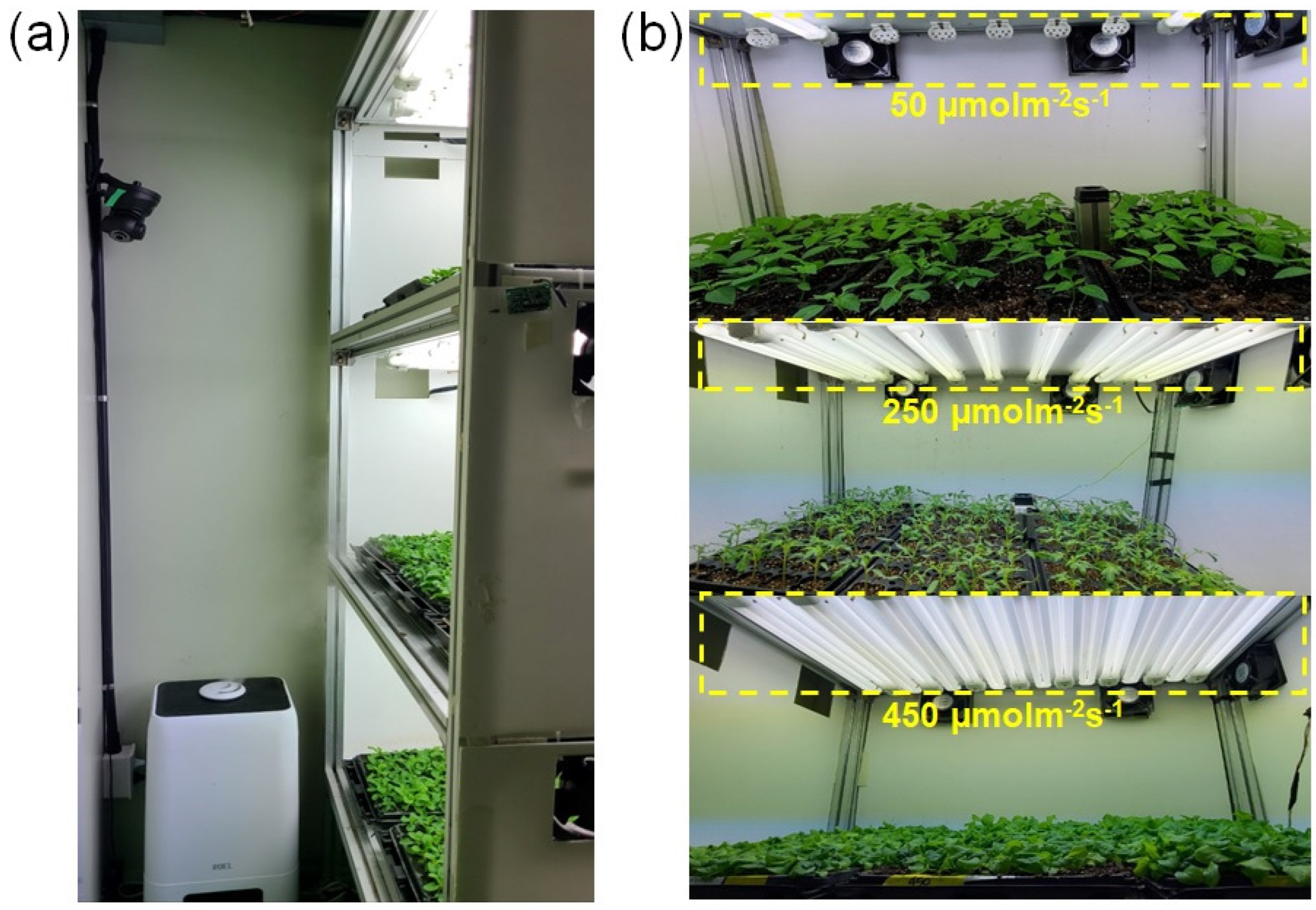
Image data collection was carried out using a low-cost commercial camera setup, as illustrated in Figure 1, with system specifications provided in Table 1. The camera (Raspberry Pi camera, Raspberry Pi Foundation, Cambridge, UK) was used to capture top-view images of seedling beds and positioned vertically 0.60 m above the seedlings to achieve a maximum field of view (FOV) of the seedling tray, with the lighting conditions kept constant for each capture. Image capture was automated using a microcontroller (Raspberry Pi 4B, Raspberry Pi Foundation, Cambridge, UK) with an integrated display, allowing seamless connectivity with the camera and facilitating automatic image capture and storage [40,41]. Images were captured daily at 14:00 h and saved in JPG format with a resolution of 3280 × 2464 pixels on an external memory card (SanDisk Ultra microSDHC Memory Card, SanDisk Corporation, Milpitas, CA, USA) connected to the microcontroller. To minimize the effects of the camera shaking or taking unfocused images, three images were taken for each seedling bed, and the average of these images was used for further analysis.
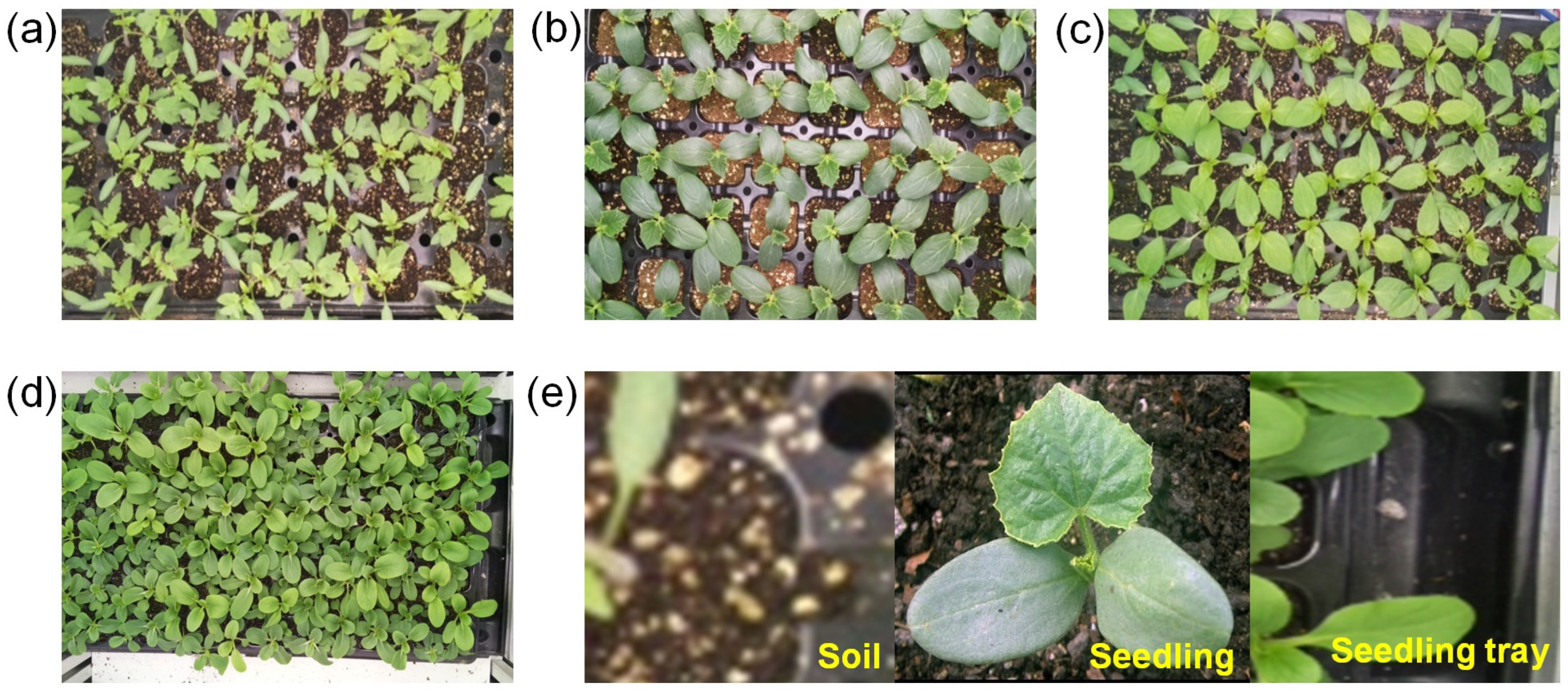
This study carefully examined the impact of lighting conditions on the four different types of seedling (tomato, pepper, cucumber, and watermelon) in controlled environmental conditions. This research focused on one of the key environmental variable affecting seedling health, light intensity, for four different types of seedling, pepper, tomatoes, watermelon, and cucumber, as shown in Figure 2. The experiment was designed to evaluate whether different lighting conditions affected the precision and efficiency of seedling segmentation using imaging processing methods. Three distinct lighting environments (50, 250, and 450 µmol·m⁻2·s⁻1) were utilized to ascertain any variance in segmentation quality, providing a detailed understanding of how light impacts not only plant growth, but also the technical aspects of plant imaging and analysis. These findings align with previous research, indicating that light intensity significantly affects seedling morphology and can influence the efficacy of segmentation techniques used in agricultural applications [41].

2.2. Dataset Preparation

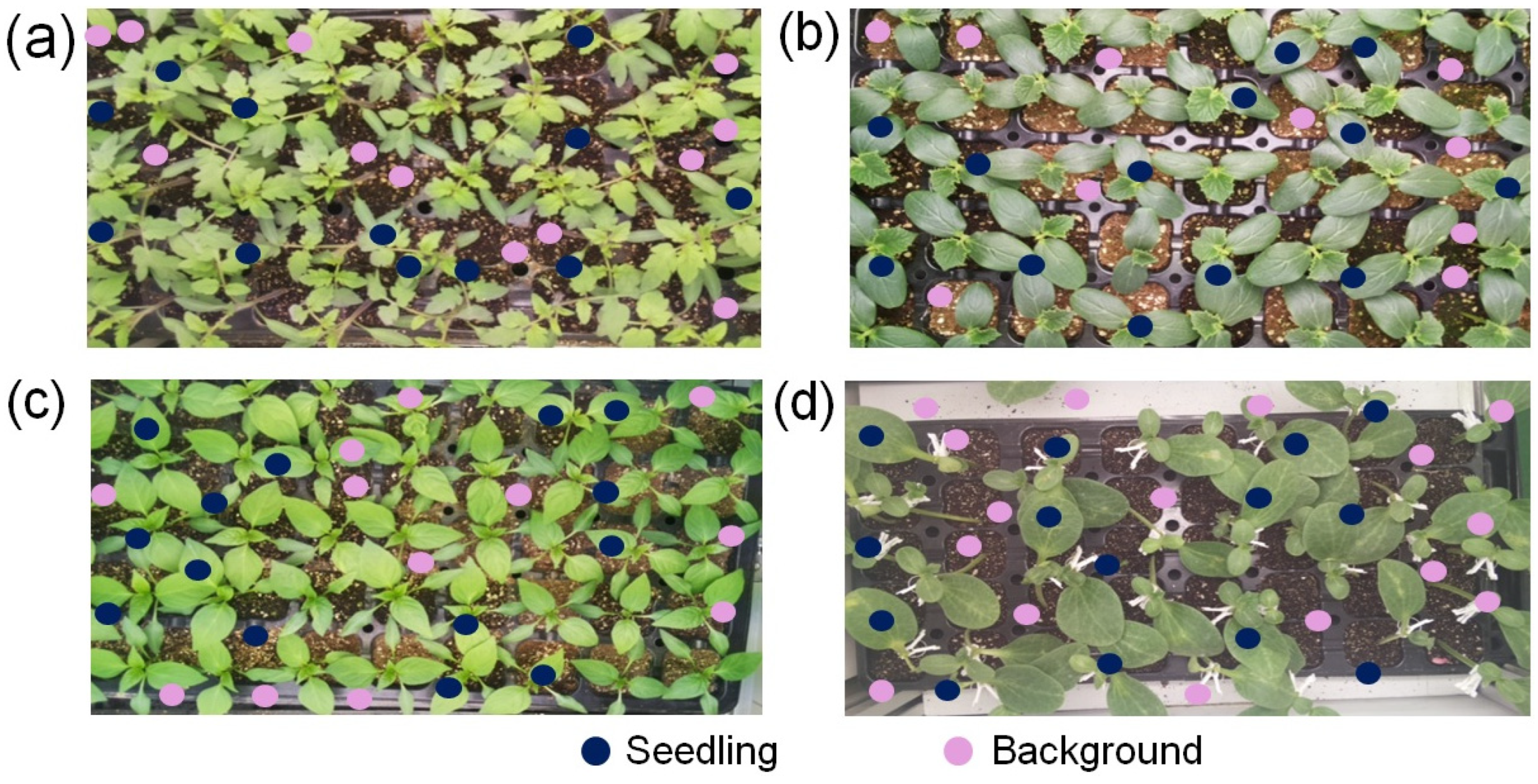
The captured images were retained at their original resolution to optimize segmentation quality, as high-resolution images minimize distortion and noise, thereby improving accuracy. Segmentation targeted the isolation of seedlings against two background types: the tray and soil. Figure 3 demonstrates the adaptability of the segmentation method by showcasing four seedling varieties under three distinct lighting conditions.
Over the 15-day experiment, a total of 900 seedling images were collected, with 15 images taken daily for each of the four seedling types, capturing three replicates per type each day. Replication was conducted to assess the effectiveness of the lighting setup and its impact on segmentation performance. As the days progressed, the seedling canopy size increased, eventually covering most of the tray area by the final day. Daily image capture allowed for monitoring background coverage and evaluating the effect on segmentation accuracy, ensuring that background presence did not interfere with effective segmentation.

2.3. Image Processing Procedure

Image preprocessing plays important role in enhancing image quality and extracting accurate information. Low-quality images often provide misleading data, complicating analysis and interpretation [7,42]. In contrast, high-quality images capture fine details, facilitating precise feature extraction and interpretation [42]. Additionally, sensor-acquired data typically contain noise, which if left unfiltered or uncorrected, can adversely affect the subsequent processing steps [43,44].
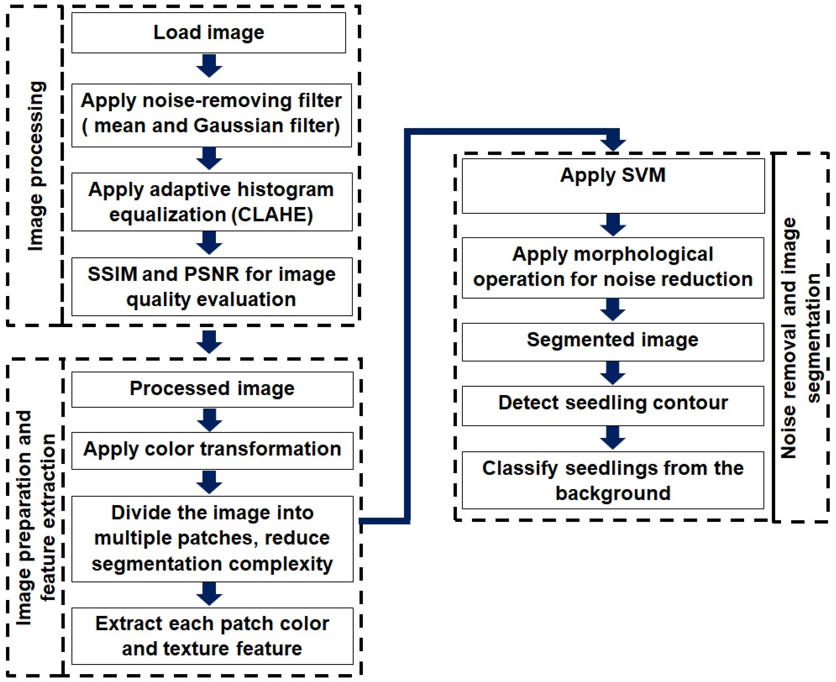
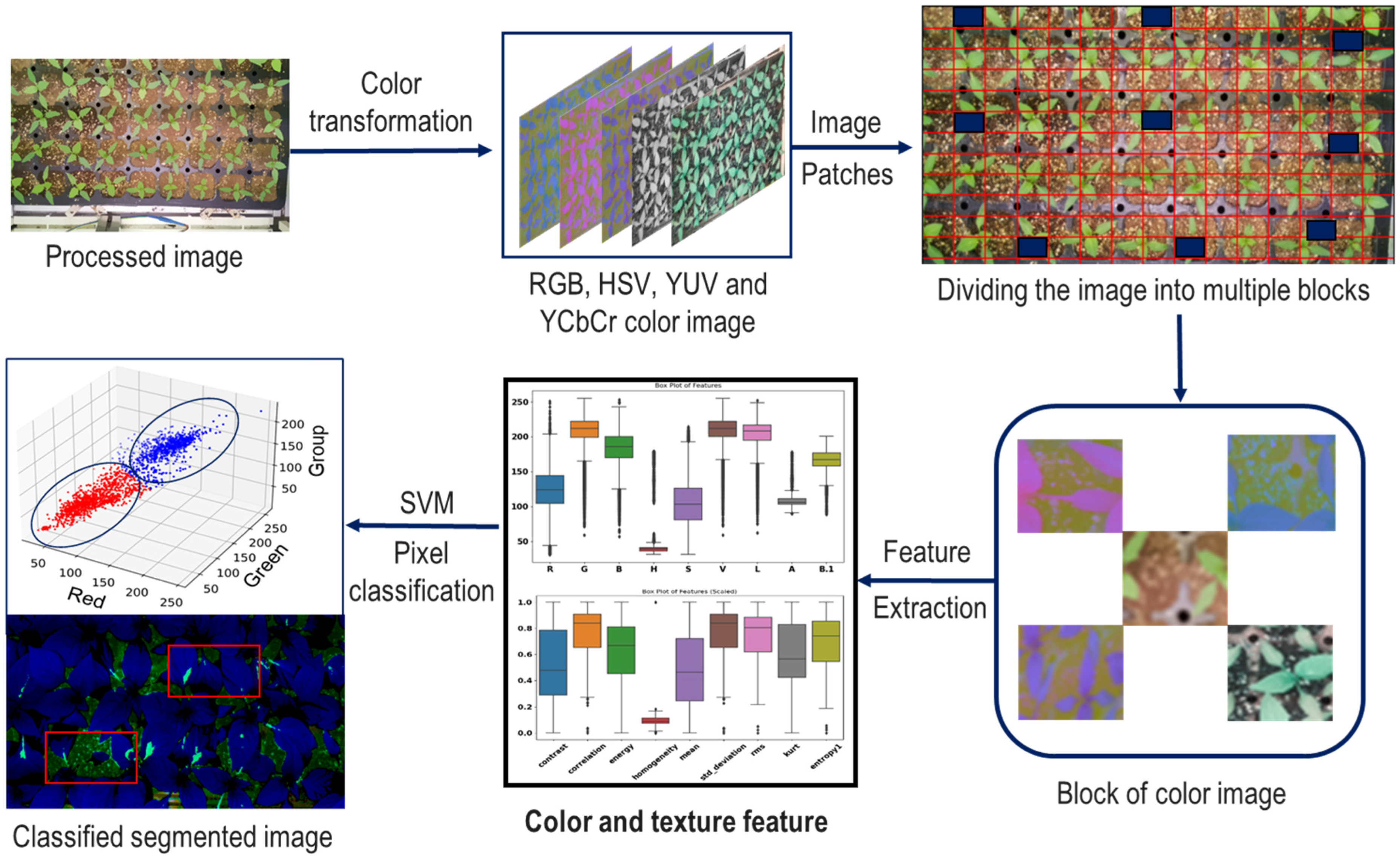
In this study, the initial preprocessing involved the application of mean and Gaussian filters to remove noise, reduce blurriness, and enhance image sharpness, improving segmentation and analysis quality. Histogram equalization was applied to minimize the lighting variations and enhance local contrast and detail visibility, leveraging intensity value distributions for improved image quality [43,44]. To address the noise amplification issue inherent in adaptive histogram equalization (AHE) [45], contrast-limited adaptive histogram equalization (CLAHE) was used. CLAHE operates on small regions (tiles) of an image, equalizing their histograms with a clip limit to prevent noise over-amplification. Bilinear interpolation was then applied to blend the tile borders, ensuring smooth transitions [46,47]. Figure 4 illustrates the complete preprocessing and feature extraction workflow used in this study.
To determine the optimal clip limit for histogram equalization, image quality was assessed using the peak signal-to-noise ratio (PSNR) and the structural similarity index measure (SSIM) across a clip limit range of 0.1 to 1.5. The PSNR quantifies the ratio between signal and noise, while the SSIM evaluates image quality by comparing the structural, luminance, and contrast features [48]. These metrics are essential for generating high-quality images, crucial for accurate seedling contour detection.
Initially, the original images were divided into multiple color channels, and CLAHE was applied to each channel with varying clip limits. The PSNR and the SSIM were measured for each value to evaluate image quality after equalization. The results indicated that lower PSNR values and higher SSIM scores correlated with better image quality. At a clip limit of 0.8, the SSIM reached 0.97, and the PSNR was 0.29, as shown in Figure 5a, demonstrating improved object–background separation. These findings align with Azam et al. [48], who observed that higher PSNR values indicate noisier or distorted images, and Sridhar et al. [49], who reported better image quality and a reduced mean square error (MSE) with lower PSNR values. Equations (1)–(3) were utilized to calculate the image quality metrics for various clip limits [50].
PSNR = 0 log 10 2 n 1 2 MSE π r 2
MSE   = 1 MN i = 0 M 1   j = 0 N 1 [ I i , j K i , j ] 2
SSIM x , y = 2 μ x μ y + C 1 2 σ xy + C 2 μ x 2 + μ y 2 + C 1 σ x 2 + σ y 2 + C 2
where n is the bit depth of the image, which determines the range of pixel values (e.g., for 8-bit images, values range from 0 to 255) and r represents the scaling factor or radius. M and N are the image dimensions, I(i,j) is the pixel value at position (i,j) in the original image, and K(i,j) is the corresponding pixel in the processed image [49]. μx, and μy are the mean pixel intensities of images I and K, while σ2x and σ2y are the variances, σxy represents covariance between the images, and C1 and C2 are constants to stabilize the formula and prevent division by zero [50].
The histogram equalization technique was used to achieve optimal contrast and improve background segmentation by mitigating the effects of uneven illumination. As illustrated in Figure 5b,c, the original images were divided into red (R), green (G), and blue (B) channels, and a clip limit (CL) of 0.8 determined through PSNR and SSIM analysis was applied to each channel. Following the application of CLAHE, the R, G, and B channels were recombined to reconstruct the original images, resulting in a histogram-equalized output with enhanced contrast.
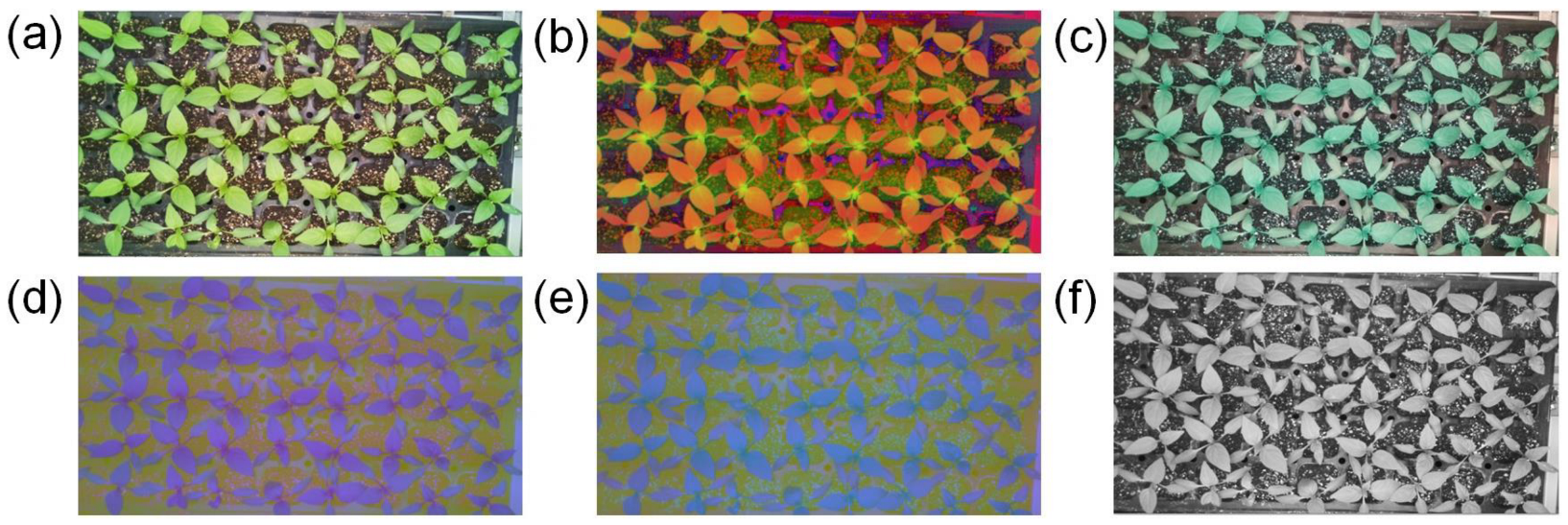
Color and textural features are widely used in agricultural research for evaluating product quality and identifying plant characteristics. Color, a key attribute related to plant physiology, aids in segmentation, stress assessment, disease detection, and other machine vision tasks [51]. Color features are intuitive and effective for isolating plant parts [52], and transforming images into different color spaces enhances the segmentation accuracy by highlighting distinguishable attributes [53]. In this study, the images were converted into six different color spaces, improving the distinction and separation of color components. This transformation facilitated more accurate feature extraction and segmentation by emphasizing specific color attributes that were less discernible in the original color space. Figure 6 illustrates the results of these transformations across various seedling types.
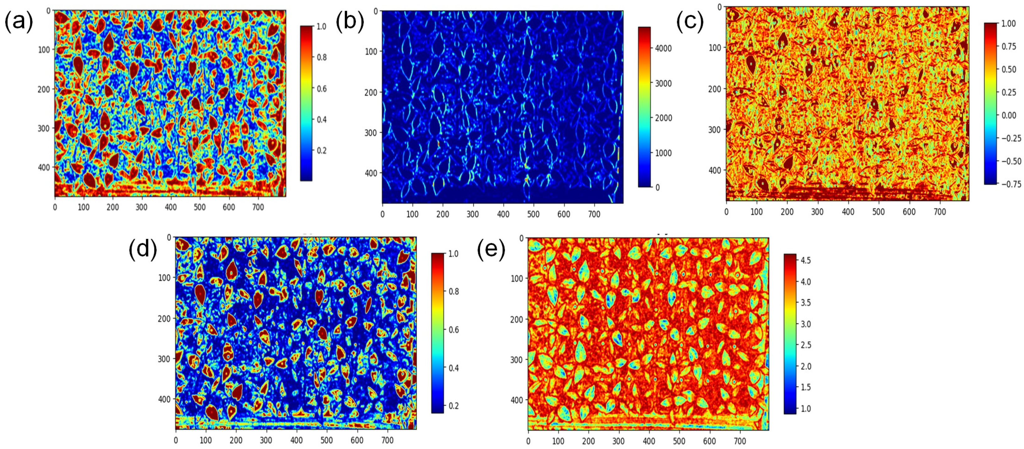
Texture features represent the spatial patterns and arrangements of pixel intensities that characterize the structure of objects in an image. In this study, texture analysis was performed using the gray-level co-occurrence matrix (GLCM), a second-order histogram that captures the spatial relationship between pixel pairs [54,55]. A flow diagram of the texture feature extraction process is presented in Figure 7. Six texture features—contrast, correlation, energy, homogeneity, mean, and entropy—were extracted from the GLCM at four orientation angles (0°, 90°, 180°, and 360°) for each image, as shown in Figure 8 [56,57,58]. Contrast quantifies local intensity variations, with higher values indicating greater differences between the neighboring pixels. Correlation measures the relationship between the neighboring pixels, with values ranging from −1 (strong negative correlation) to 1 (strong positive correlation). Energy, or angular second moment, reflects uniformity, while homogeneity evaluates the proximity of GLCM elements to its diagonal, with values ranging from 0 to 1. Entropy assesses the randomness or complexity of the texture, indicating greater variability with higher values. These features were derived from an 18-color system, and the SFS method was applied to identify significant differences among them.

2.4. Feature Pattern and Feature Selection

Graphical representations of data provide an intuitive means to identify patterns, relationships, and outliers within features, offering insights that raw data alone cannot reveal. Three dimensional (3D) visualizations, as shown in Figure 9a, add depth to analysis, offering a comprehensive view of data interactions. Similarly, hierarchical clustering dendrograms, as shown in Figure 9b, represents hierarchical relationships among the data points, facilitating the identification of clusters and feature similarities. These visualization tools simplify complex datasets, enhance interpretability, and support informed decision making by identifying multicollinearity and guiding feature selection for further analysis.
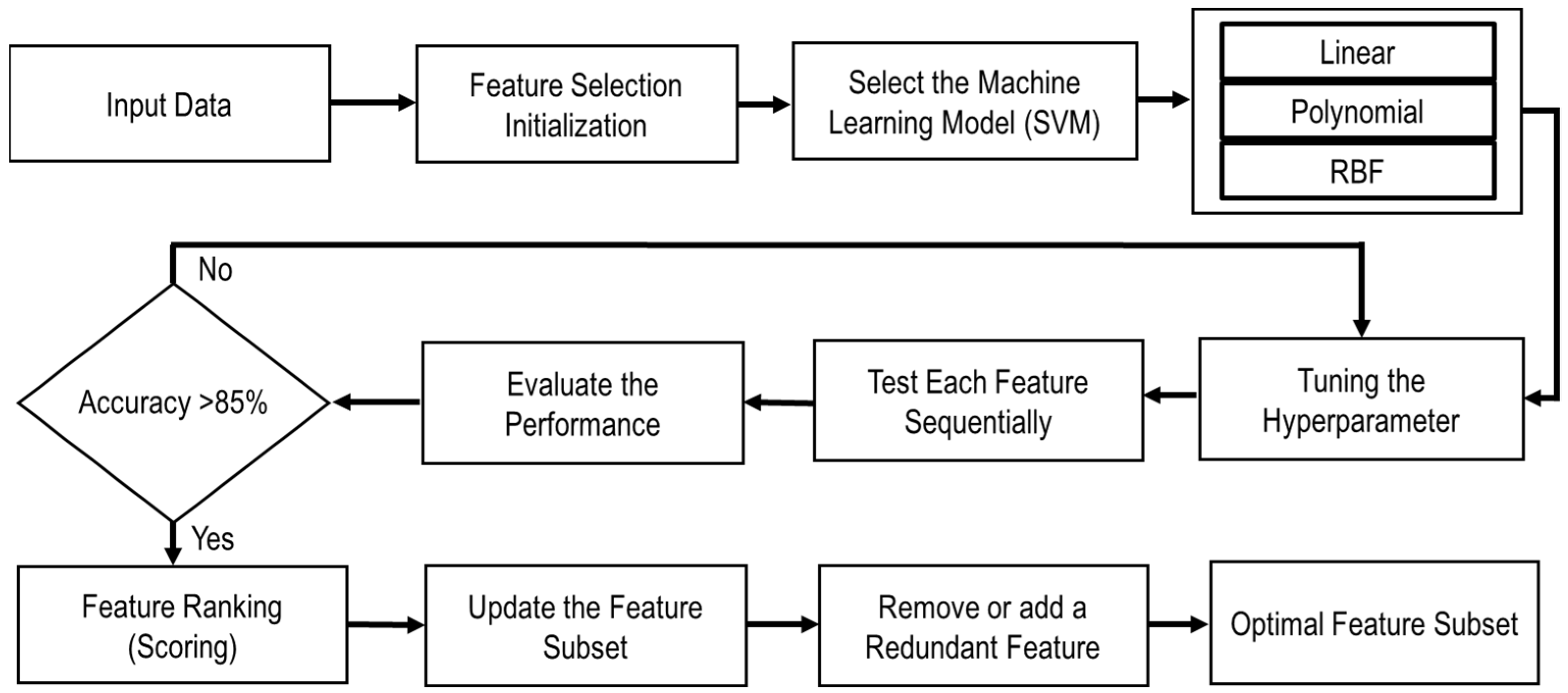
Feature selection is an essential process in machine learning and image analysis, particularly for agricultural applications, as it reduces data dimensionality, enhances the model’s performance, and improves computational efficiency [59,60]. By selecting the most informative features, redundant or irrelevant features that increase noise and complexity are eliminated [60]. In this study, 24 features, including color and texture attributes, were extracted from the seedling images. While these features provide valuable information, using all of them risks overfitting and computational inefficiency [61]. To address this, the sequential feature selection (SFS) method was employed to identify the most relevant features.
As illustrated in Figure 10, SFS begins with an empty feature set and iteratively adds features based on their contribution to model accuracy. At each iteration, the features are evaluated and ranked, with only those significantly enhancing the classification performance retained. The process continues until the optimal subset of features is selected, which is then used to build the final classification model. Using a linear regression framework, SFS effectively removes the redundant features and identifies those most relevant for segmentation [62]. In this analysis, SFS streamlined the model by excluding the less-informative features, thereby enhancing the performance of the SVM classifier. This optimization improved segmentation accuracy for seedling images, a crucial requirement for real-time agricultural monitoring [63].

2.5. SVM Segmentation Model

Image segmentation partitions an image into multiple segments to simplify representation and facilitate analysis, typically for object localization and boundary allocation [64]. By grouping pixels with similar attributes, segmentation creates a pixel-wise mask, enabling the clearer understanding of objects within an image.
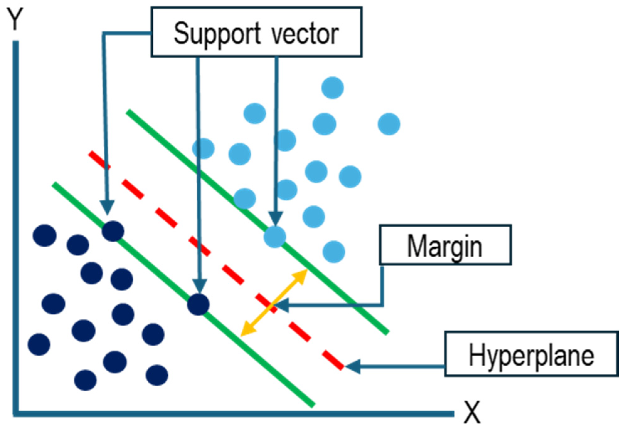
The SVM is highly effective supervised learning algorithm widely used for classification, regression, and outlier detection. The SVM identifies an optimal hyperplane that maximizes the margin between classes, ensuring robust classification [7]. The margin, defined as the distance between the hyperplane and the nearest data points (support vectors), is critical for determining the hyperplane’s orientation and position. By maximizing this margin, the SVM improves generalization and performs effectively on unseen data, particularly for linearly separable datasets. Figure 11 illustrates the role of support vectors in defining the hyperplane.
Many real-world datasets, including those for image segmentation tasks like seedling classification, are not linearly separable. To address this, the SVM employs kernel functions to transform the input space into a higher-dimensional space, enabling linear separation through the “kernel trick”, without explicitly computing the transformed coordinates [65]. The linear kernel suits linearly separable data, while the polynomial kernel captures complex non-linear relationships. The radial basis function (RBF) kernel, widely used in image segmentation, efficiently handles non-linear separations by mapping data into higher dimensions using a Gaussian function, making it particularly effective for variations in lighting, texture, and structure in seedling segmentation [66,67].
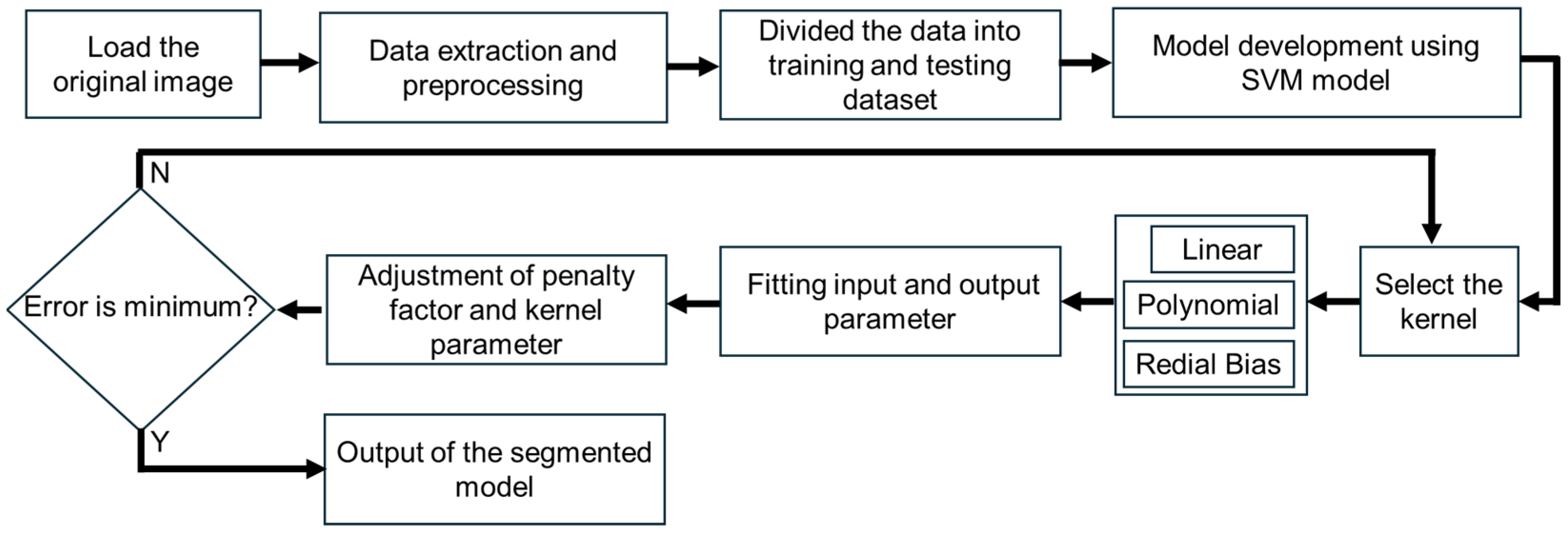
The SVM algorithm presented in this study is distinguished by its integration of feature selection, hyperparameter tuning, and the application of kernel functions, including linear, polynomial, and radial basis functions (RBFs). The development of the SVM classification model follows a structured and iterative process to maximize accuracy and performance, as outlined in Figure 12. The process begins with data acquisition, followed by preprocessing to clean, normalize, and structure the data for consistency. The dataset is then split into training and test sets to facilitate model development and evaluation. An initial SVM model is constructed using the training set, with the choice of kernel function (linear, polynomial, or RBF) based on data complexity. The kernel transforms the data into a higher-dimensional space, enabling effective decision boundaries, particularly for non-linear patterns.
Hyperparameter tuning is conducted iteratively to optimize parameters, such as the penalty factor (C) and kernel-specific settings, minimizing fitting errors. This refinement continues until the error is reduced to an acceptable threshold. The final optimized SVM model is then deployed for segmentation tasks, delivering high accuracy and a robust performance.

2.6. Overall Image Segmentation Process

Following image processing, the images were converted into multiple color spaces (RGB, HSV, YCbCr, YUV, LUV, and XYZ) to capture diverse color information. Each image was divided into patches representing foreground (seedlings) and background (soil and pots) areas to simplify segmentation and focus on the key features. This patch-based approach reduced complexity and preserved critical edges and details, ensuring high accuracy in seedling segmentation and classification.
As shown in Figure 13, sampling points for pixel information were randomly selected from both the foreground and background regions. Color and texture information was extracted from these points, capturing a broad range of variations. This detailed sampling enabled the model to differentiate the seedlings from the background effectively, improving the segmentation accuracy. The comprehensive coverage of image features facilitated precise pixel classification for accurate seedling segmentation.
In this study, each seedling image was divided into ten tiles, with five patches extracted from the foreground (seedling) and five from the background (soil and pots). This approach enabled the model to differentiate seedling from background pixels, while reducing the complexity arising from varying colors and textures. Using 225 images per seedling type (pepper, tomato, cucumber, and watermelon), a total of 2250 tiles (10 tiles per image × 225 images) were generated for each type, providing a diverse dataset to improve segmentation accuracy.
Color and texture features were extracted from each tile to create a comprehensive feature set for training the SVM model. The SVM-classified pixels, as either seedling or background, achieving precise segmentation. The dataset was split into 80% for training and 20% for testing, ensuring model robustness and generalization to the new data [68,69]. The complete seedling segmentation process, encompassing feature extraction and classification, is illustrated in Figure 14.
After pixel classification, morphological operations were applied to remove noise, fill gaps, and refine the boundaries of the segmented images. These operations, designed for binary images, enhance the spatial coherence of pixel values, improving the visual quality of segmentation. The refined seedling contours were then extracted from the segmented masks and converted into annotated boundary files, enabling real-time object detection and monitoring. These annotations are critical for different applications, such as training object detection models (e.g., YOLO) or monitoring plant health in real-time agricultural systems.

2.7. Performance Evaluation for Boundary Contour Determination

This study focuses on contour determination during background segmentation using color and texture features with SVM. The background segmentation accuracy was evaluated using precision, recall, F1-score, accuracy, confusion matrix, and leaf area measurement. For real-time detection, annotation files were generated from the image dataset contours. The segmentation performance was assessed using a confusion matrix to analyze the true positives (TPs), false positives (FPs), true negatives (TNs), and false negatives (FNs). TPs represent correctly segmented positives, FPs are negatives misclassified as positives, TNs are correctly segmented negatives, and FNs are positives misclassified as negatives [7]. Precision, recall, F1-score, and accuracy were calculated using standard equations [64], ensuring the comprehensive evaluation of segmentation performance as follows:
Precision = TP TP + FP
Recall = TP TP + FN
F 1 _ score = 2 * Precision * Recall Precision + Recall
Accuracy = TP + TN TP + TN + FP + FN
Leaf area is an important metric for validating segmentation model accuracy. It enhances precision by isolating the leaf regions, ensuring accurate boundaries, reducing misclassification, and filtering irrelevant background elements. This is particularly crucial as segmentation processes may risk boundary reduction or object loss due to morphological erosion. Wang et al. [67] highlighted this issue in a multi-stage image-processing technique for cell segmentation, where excessive erosion led to reduced cell sizes and the occasional loss of cells. To prevent similar inaccuracies, maintaining accurate leaf boundaries is essential for reliable segmentation models.
Preparing annotation files from the extracted contours is crucial for evaluating the contour accuracy and reducing annotation time in real-time object detection and monitoring tasks. Vădineanu et al. [68] addressed the high labor costs of manual annotation in cell image segmentation, proposing contour-based masking to accelerate the process. While this method reduces effort, it may compromise precision in certain cases. Similarly, Lu et al. [69] introduced a contour transformer network for image segmentation, converting contours into annotation files for anatomical structure segmentation, demonstrating the utility of automated annotation in enhancing efficiency and accuracy.
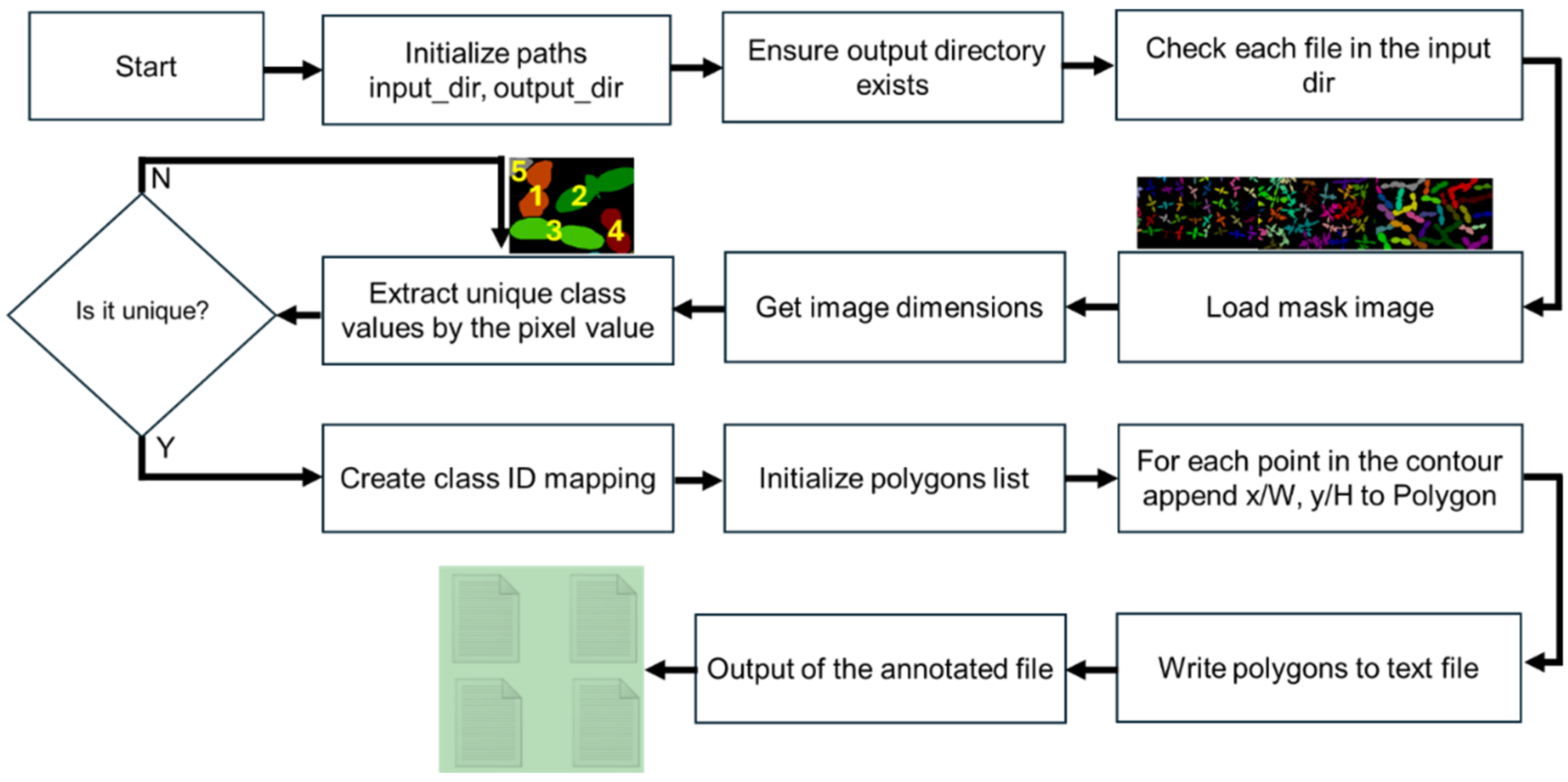
Figure 15 illustrates the process of preparing the annotation files from the contour image dataset. The procedure begins with loading the mask images in grayscale to identify multiple classes and extracting the unique class values, while excluding the background. Original class IDs are mapped to the new sequential IDs, and binary masks are created for each class to isolated objects. Contour points are normalized by dividing by the image dimensions, ensuring annotations are independent of image size. Contours with an area below a defined threshold are excluded to retain only the meaningful objects. The normalized contour points and class IDs are then saved as text files for each image, providing precise, scalable annotations essential for training object detection and segmentation models.

3. Results

3.1. Selected Features

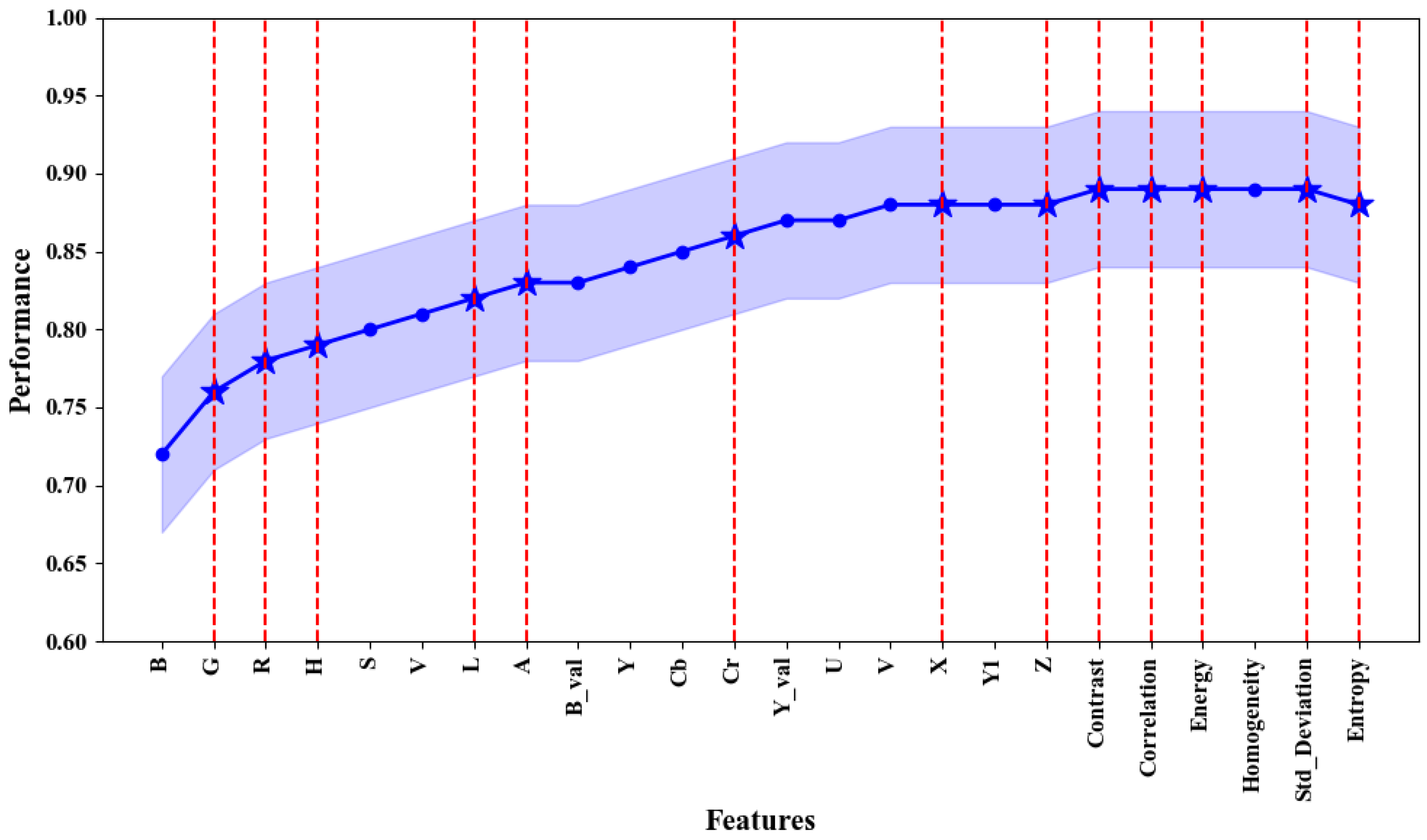
To optimize the boundary contour determination-based segmentation method during the background removal process, a total of 24 features were used for this task, comprising 18 colors, and 6 textures features. The goal was to prevent overfitting by identifying and eliminating the irrelevant or redundant features. To achieve this, the SFS method was applied, systematically selecting and evaluating the feature subsets for their effectiveness in enhancing background segmentation. The method identified a subset of 13 key features as the most influential in accurately separating the seedlings from the background. The use of these 13 features significantly improved the segmentation accuracy, as demonstrated in Figure 16, which highlights the contribution of the selected features to the improved segmentation process. From the original 24 features, the selected 13 features contributed to a more efficient and accurate segmentation model.

3.2. Performance of the SVM Segmentation Model

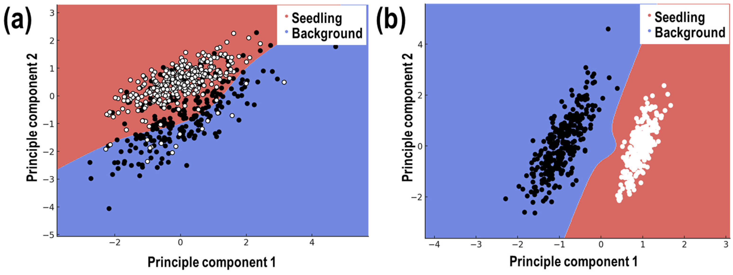
Before applying any optimization techniques, the classifier showed promising results. However, after refining the features, the improvement in accuracy was evident, as shown in Table 2. Figure 17 illustrates the decision boundaries of the SVM model both be-fore and after feature selection, showing a more defined separation between the seedling and background categories following optimization. Initially, 80% of the dataset was allocated for training, and 20% for testing. The dataset included 24 extracted features, such as color and texture features, which were used as inputs for the SVM classifier. For feature selection, the SVM classifier with a polynomial kernel function and five-fold cross-validation achieved an accuracy ranging from 73 to 98% using a regularization parameter of 60, a kernel coefficient of 0, and a degree of 3.
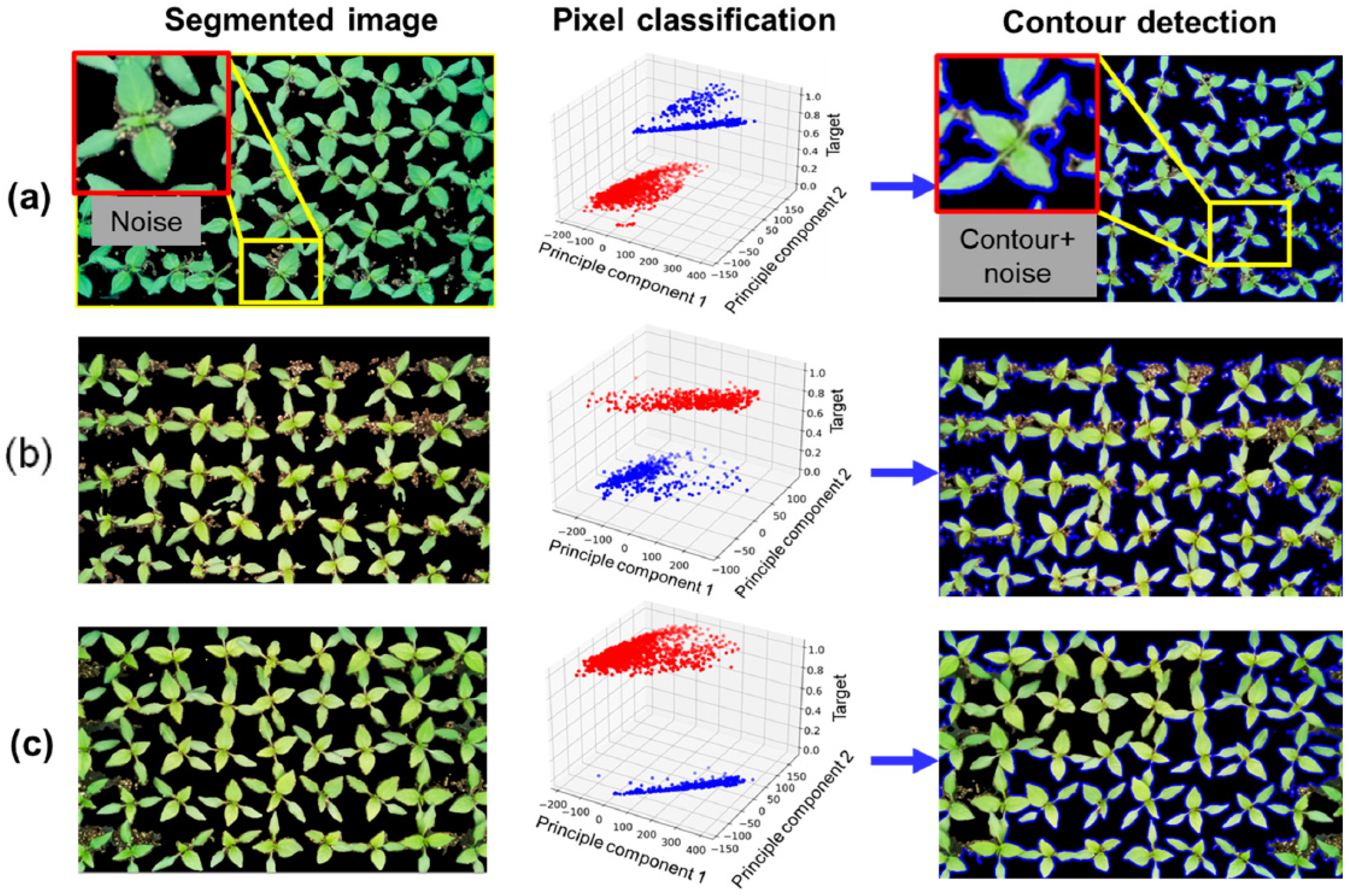
Without feature selection, the model achieved 73% accuracy, with noise prevalent in the image classification results, particularly in the contour detection around the seedlings under varying light conditions (50, 250, and 450 µmol·m⁻2·s⁻1), as shown in Figure 18. The noise led to imprecise segmentation and noisy boundaries, which hindered the accurate classification of pixels between the seedlings and the background. After applying the SFS method for feature selection, the classifier’s accuracy increased significantly to 98%, as shown in Table 2. This improvement not only enhanced the classification accuracy, but also reduced the noise levels in the segmented images, leading to clearer and more accurate contours, as highlighted in Figure 19. This underscores how focusing on the most informative features can enhance the classification accuracy and improve the overall segmentation quality by eliminating irrelevant or redundant data.
In this study, the SVM was used for classifying the seedlings from the background due to its ability to handle complex, high-dimensional datasets [70]. The SVM identified the optimal hyperplane to maximize the margin between classes, enabling robust separation. Kernel functions, including RBF, linear, and polynomial, were applied to transform the data into higher-dimensional spaces, effectively managing both linear and non-linear patterns [71]. The RBF proved particularly effective for capturing the non-linear patterns of the dataset. To enhance accuracy and generalization, 0-, 5-, and 10-fold cross-validation was used, reducing overfitting by testing the model on various data subsets and ensuring a better performance on unseen data [71,72]. The regularization parameter (C) was adjusted to balance margin maximization and classification error minimization, improving the model’s accuracy and robustness to noise [73,74,75].
Figure 20 displays the decision boundaries for the SVM model using different cross-validation folds and regularization parameters. The polynomial kernel provided the highest accuracy of 98%, with recall at 97%, an F1-score of 98, and precision at 98%, as illustrated in Table 3. Without cross-validation, both the linear and RBF kernels demonstrated a similar performance in distinguishing the seedlings from the background, with an accuracy of 81%, a recall of 81%, and a precision of 80%. The polynomial kernel, on the other hand, slightly outperformed these, achieving an accuracy of 86%, a recall of 86%, and a precision of 85%. The higher precision in the polynomial kernel indicates its ability to make accurate positive predictions, though it slightly underperformed in recall, suggesting that some positive instances were missed. With five-fold cross-validation, all the kernel functions showed significant improvements in classification accuracy. The polynomial kernel achieved the highest accuracy of 98%, with a precision of 98% and a recall of 97%. In contrast, the linear and RBF kernels performed similarly, each achieving an accuracy of 96%, with both precision and recall values of 95% and 96%, respectively. In the 10-fold cross-validation, all the kernels exhibited similar classification accuracy, with the polynomial, RBF, and linear kernels achieving an accuracy of 88%. Both the polynomial and RBF kernels had precision and recall values of 88%, while the linear kernel slightly lagged with a precision and recall of 87%. These results are shown in Table 3 and Table 4.
Overall, the polynomial kernel consistently outperformed the others in precision, highlighting its capability to make accurate positive predictions. However, its recall was slightly lower, indicating that while it accurately identified positive instances, some were overlooked. The regularization parameters (C and γ) also played a critical role in the model’s performance. Higher values of C and γ led to significant improvements in accuracy, particularly with the polynomial kernel, where C of 60, γ of 0, and a degree of 3 resulted in notable gains in accuracy (Table 4). Conversely, lowering C and γ to 128 resulted in a decrease in performance across all the kernels. These findings underscore the importance of tuning regularization parameters to optimize the SVM performance across different kernel functions and cross-validation strategies.
After image classification using the SVM model, the segmented images were further processed for contour optimization to enhance the segmentation accuracy. The primary purpose of contour optimization is to refine the seedling boundaries and ensure that no parts of the seedlings are cut off or inaccurately segmented. This process is crucial for calculating the exact area occupied by each seedling, as well as for generating precise annotations. Various morphological operations, such as dilation and erosion, were applied to eliminate noise and smooth the contours, ensuring clean and continuous boundaries. Contour determination is especially important in image segmentation for seedling health monitoring because it directly affects the precision of area measurements and annotations, which are critical for evaluating seedling growth and health. Other studies have shown that determination of contours enhances both the reliability of annotations and the overall accuracy of classification tasks, making it a valuable step in real-time monitoring systems [14].
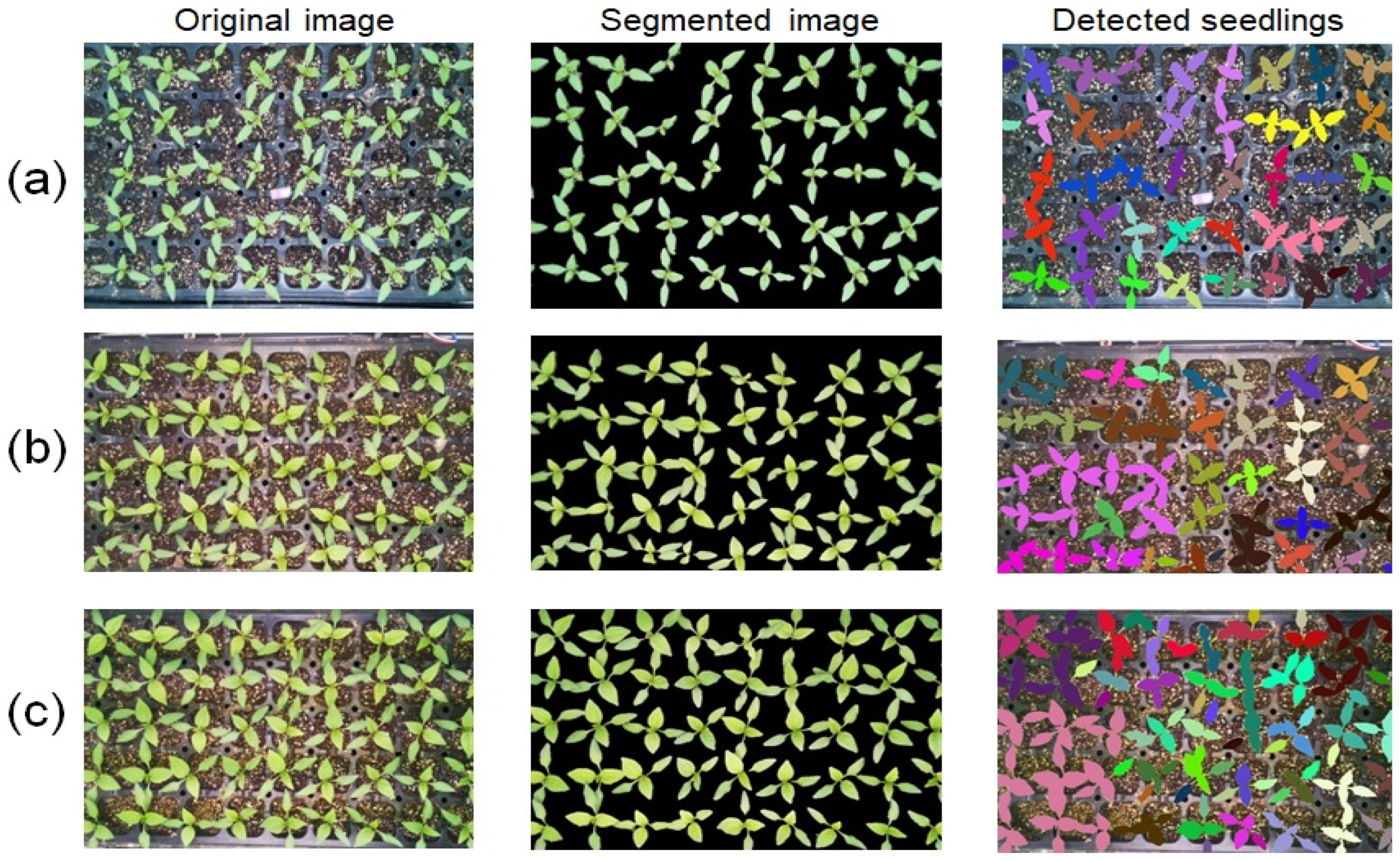
First, the segmented image was processed to generate a segmented mask. This mask was then used to extract the contours of the seedlings. Once the contours had been identified, they were drawn onto the image, followed by the generation of bounding boxes around each seedling based on the contour boundaries. The resulting images with refined contours and bounding boxes, as shown in Figure 21, highlight the accuracy and effectiveness of this method. Contour optimization improved the visual clarity and accuracy of segmented images, leading to more precise annotations for real-time seedling health monitoring. This step ensured that contours aligned with actual seedling shapes, enhancing the segmentation quality and data reliability for further analysis.

3.3. Segmentation Performance Evaluation

The segmentation performances of the different seedlings were evaluated using the precision, recall, F1-score, and accuracy metrics, as shown in Table 2 and Figure 22. Initially, the segmentation results showed a moderate performance before the application of feature selection techniques. For pepper seedlings, the precision was 87%, the recall was 86%, the F1-score was 87%, and the overall accuracy was 87%. The tomato seedlings had a precision of 81%, a recall of 77%, an F1-score of 77%, and an overall accuracy of 77%. The cucumber seedlings achieved a precision of 83%, a recall of 81%, an F1-score of 80%, and an overall accuracy of 81%. The watermelon seedlings showed a precision of 86%, a recall of 83%, an F1-score of 82%, and an overall accuracy of 82%, as shown in Table 2, without the SFS method.
After applying the SFS method for feature selection, the segmentation performance improved significantly. The pepper seedlings showed a precision of 96%, a recall of 99%, an F1-score of 98%, and an overall accuracy of 98%. The tomato seedlings achieved a precision of 97%, a recall of 98%, an F1-score of 98%, and an overall accuracy of 98%. The cucumber seedlings reached 99% precision, 100% recall, a 99% F1-score, and 99% overall accuracy. Finally, the watermelon seedlings demonstrated precision of 97%, a recall of 97%, an F1-score of 97%, and an overall accuracy of 97%, as shown in Table 2, with the SFS method. This illustrates the impact of feature selection on enhancing classification accuracy and segmentation quality.
The performance of the SVM model was evaluated using the confusion matrix and the ROC curve. The ROC curve, a graphical representation of the TPR versus FPR, was utilized to assess the performance. Among the tested kernels, the polynomial SVM model achieved the highest accuracy of 98% with a threshold value of 0.55, as shown in Figure 22c. The confusion matrices in Figure 22a(1–4) represents the classification results for pepper, tomato, cucumber, and watermelon before feature selection. For instance, the pepper seedlings (Figure 22a(1)) show 516 TPs, 77 FNs, 84 FPs, and 523 TNs. After feature selection, the confusion matrices (Figure 22b(1–4) show improvement in the classification results, with the pepper seedling (Figure 22b(1)) showing 594 TPs, 24 FNs, 6 FPs, and 576 TNs. The polynomial kernel performed better than other kernel-based SVM models in classifying the binary data, demonstrating superior accuracy and a classification ability. The polynomial kernel model was particularly effective in distinguishing between the classes, further solidifying the superiority in this study.
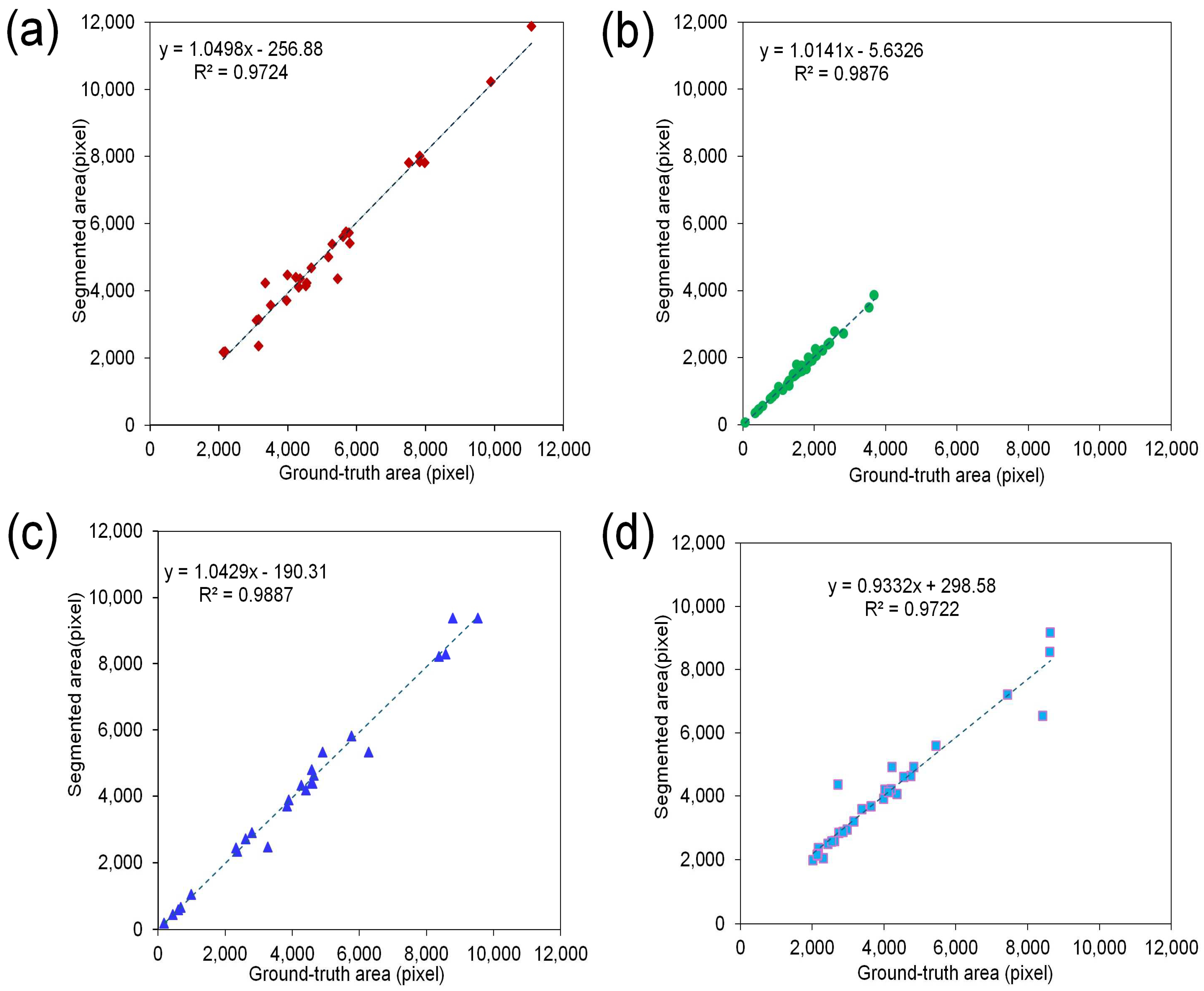
In Figure 23, the validation results demonstrate the high accuracy and reliability of the proposed segmentation method across different seedling types under varying lighting conditions (50, 250, and 450 µmol·m⁻2·s⁻1). R2 indicates a strong correlation between the actual ground truth canopy area and the segmented canopy area. Specifically, the R2 values were 0.98 for the pepper seedlings, 0.98 for the tomato seedlings, 0.97 for the cucumber seedlings, and 0.97 for the watermelon seedlings. These high R2 values highlight the robustness and precision of the proposed method in accurately segmenting the canopy area, regardless of light intensity, confirming its effectiveness and consistency in diverse environmental conditions.
To further evaluate the effectiveness of the proposed segmentation method by generating a contour-based annotation file, comparative analysis was conducted between the manually annotated dataset and the contour-based annotated dataset. This analysis aims to assess not only the accuracy of object detection and segmentation, but also to check how the model works when trained with the two different types of data. In this case, the YOLOv8 model was used to evaluate the performance of the deep learning framework on the proposed contour-based annotation file. Since training deep neural networks typically require a large amount of human-annotated data, which can be tedious and inefficient, alternative approaches were considered. For instance, Zhuang et al. developed an iterative deep-learning algorithm for contour-based annotation aimed at organ segmentation. They compared their model with other deep learning models and found that their method significantly reduced the annotation time and minimized inter-rater variability, outperforming other models in terms of accuracy and efficiency [14]. Similarly, Guo et al. [76] introduced a contour-based real-time strawberry instance segmentation network by employing a specific octagonal contour and deep snake convolution method. Their results demonstrated that the proposed method achieved real-time recognition with high accuracy and outperformed the other existing segmentation techniques.
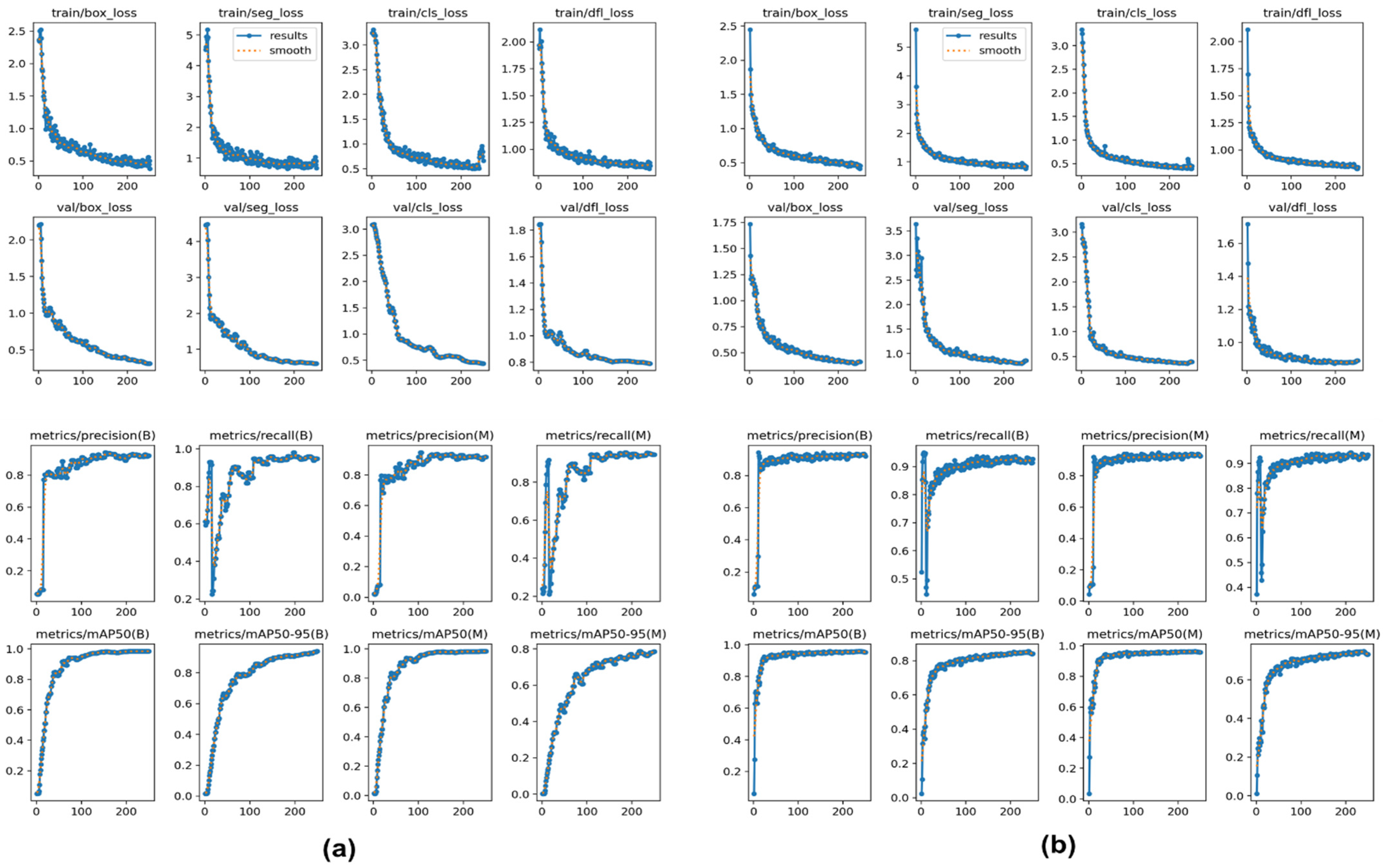
The results of the comparison revealed that the contour-based annotation data approach, as shown in Figure 24a, demonstrated significant advantages in terms of computational speed and annotation efficiency. In particular, training on the contour-based dataset resulted in faster convergence during the training phase, as evidenced by fewer training and validation losses. The training loss for the contour-based method converged faster, with a final box loss of 0.50 versus 0.55 for the manual method, indicating a more efficient learning process. Additionally, the mAP50 for the contour-based method reached 0.80 at epoch 200, while the manual method achieved 0.78, and the mAP50-95 for the contour-based method was 0.68 compared to 0.65 for the manual method, showing a slight edge in overall accuracy.
However, the manual annotation dataset showed higher precision in some respects, as shown in Figure 24b. At the end of training, the precision for the manually annotated dataset was 0.83, which is slightly higher than 0.82 achieved by the contour-based annotation method. This suggests that while the contour-based method surpassed in terms of mAP and training efficiency, manual annotation provided marginally better precision in object detection.
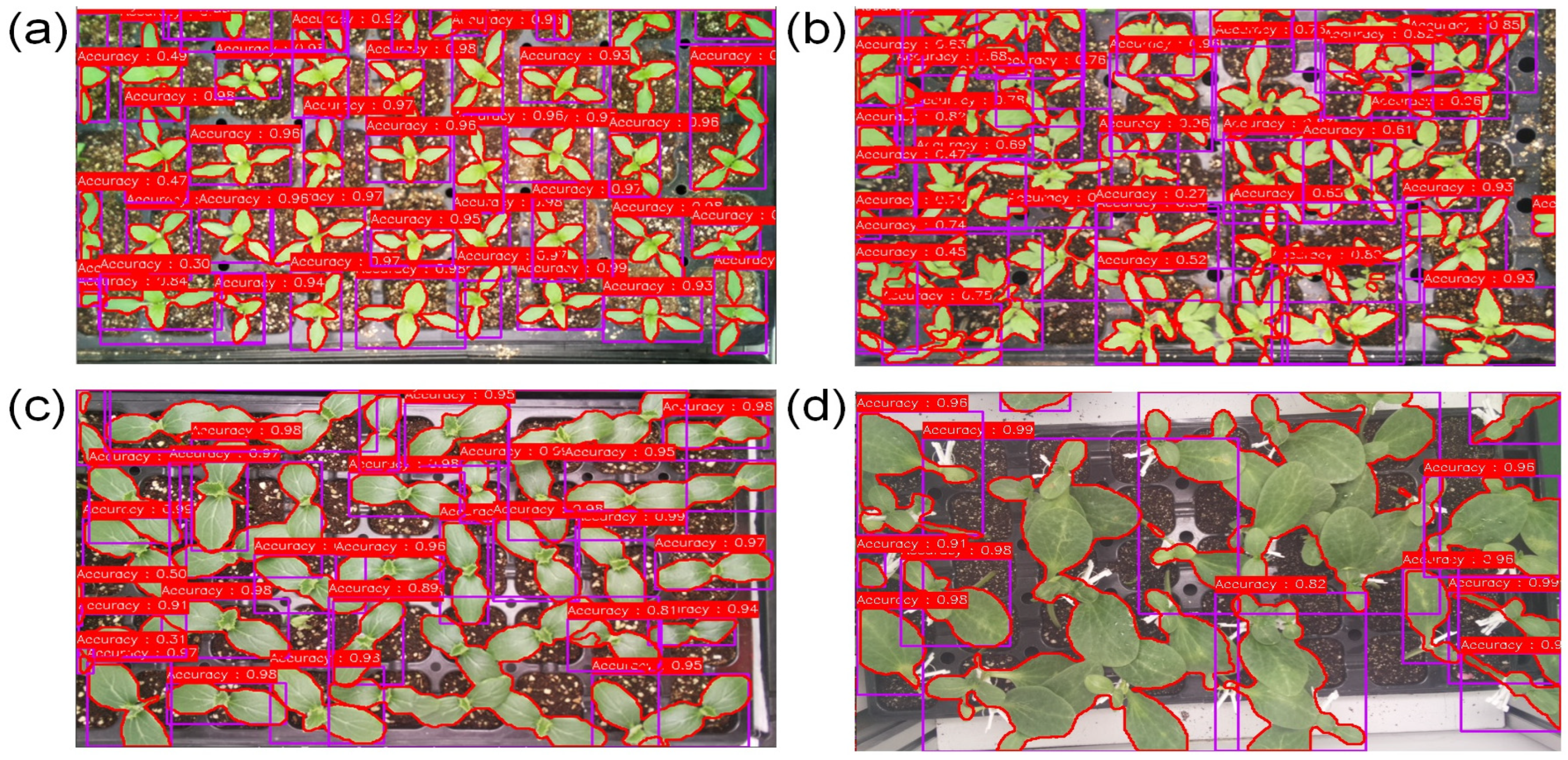
After developing and training the YOLOv8 model, it was tested on a set of unseen images that were not part of the training or validation datasets. The results shown in Figure 25 reveal that the proposed contour-based annotation method achieved high accuracy in detecting the seedlings, with the overall accuracy ranging from 96% to 98% and precision and recall rates of 96% across all the classes (pepper, tomato, cucumber, and watermelon). In comparison, the manually annotated training model demonstrated slightly higher accuracy, with accuracy rates ranging from 97% to 99% and precision and recall reaching 98%. This high level of accuracy underscores the robustness and effectiveness of the contour-based annotation method in capturing essential features required for precise object detection.
The manual annotation method precisely separated the individual seedlings, while the contour-based approach grouped the overlapping leaves. Despite this, the contour-based method delivered excellent results for object detection and segmentation, proving effective for real-time monitoring applications. Its ability to distinguish seedlings from complex backgrounds minimized the false positives and the false negatives, validating its reliability. This demonstrates the proposed method’s potential for accurate object detection, monitoring, and plant health assessment, confirming its practical utility in real-world scenarios. Figure 26 illustrates the seedling detection results using contour-based annotation with bounding boxes.
Comparative analysis was performed to evaluate the proposed method against the different segmentation models. Table 5 summarizes the segmentation accuracy achieved by the various models, including the proposed contour determination approach. The results indicate that the proposed method achieved competitive accuracy (79–98%), particularly after feature selection, showing the capability to handle structural complexities in seedling segmentation. In comparison, a similar study by Gao et al. [77] utilized OTSU and marker-based watershed algorithms for medicinal plant leaf segmentation, achieving an impressive accuracy of 99.9%. These findings highlight the strengths of the proposed method, while providing a benchmark against the existing approaches. Sadeghi-Tehran et al. [78] addressed the challenges of dynamic field conditions by developing a robust multi-feature learning model (MLF) for fractional vegetation cover segmentation, effectively overcoming issues such as varying illumination without relying on manual thresholding. Similarly, Ghosh et al. [79] achieved up to 99.5% accuracy in plant classification by integrating the CNN with the KNN, demonstrating the potential of hybrid approaches. Hossain et al. [80] focused on plant disease segmentation using texture and color features using a KNN-based approach, achieving an accuracy of 96.76%. Zhang et al. [81] tackled the complexities of irregular leaf patterns with a method that combined super pixel clustering, K-means, and PHOG descriptors, resulting in effective segmentation and disease classification.
When applied to the same dataset, the proposed method achieved an accuracy of 98%, closely matched with the CNN + KNN [77] at 99%. However, other methods, such as OTSU + watershed [75] and the KNN [78], which were effective on other datasets, struggled with the structural complexities of the proposed model’s dataset. This highlights the importance of advanced or hybrid approaches, such as the proposed method, for achieving a superior segmentation performance in complex scenarios.

4. Discussion

In this study, preprocessing techniques, such as median and Gaussian noise removal filters, contrast enhancement, and histogram equalization, were applied to minimize the effects of uneven lighting and enhance important seedling features. These methods effectively improved the image quality by addressing uneven lighting conditions, which would otherwise reduce segmentation accuracy and compromise the overall image quality [82,83].
During the preprocessing step involving histogram equalization, the PSNR and SSIM metrics were calculated for each clip limit, as shown in Figure 5c. A clip limit of 0.8 was selected based on its high SSIM value of 0.97, which indicated strong structural similarity across the different histogram equalization results of the processed images, and a relatively low PSNR value of 0.29. Previous studies, such as those by Juneja et al. [84] and Büyükarıkan et al. [85], also demonstrated that SSIM values above 0.95 ensure excellent image quality for tasks like plant disease detection, where maintaining structural details is crucial. Although PSNR values above 30 dB are generally preferred for clarity, lower PSNR values can still be acceptable if the SSIM values remain high, particularly in tasks like segmentation where maintaining structural accuracy is more important.
Feature selection played a key role in improving segmentation accuracy. Thirteen features were selected using the SFS method, focusing on the key color channels (B, G, H, L, A, Cr, X, and z) and texture attributes (contrast, correlation, energy, standard deviation, and entropy). These features effectively captured the differences between the seedlings and the background, leading to a significant improvement in the SVM classifiers performance, increasing accuracy from 73% before feature selection to 98% after. Reducing the number of features helped decrease the model’s complexity and prevent overfitting, while retaining the essential information needed for accurate segmentation. The SFS method ensured that only the most relevant features were retained, reducing the computational cost and boosting the segmentation accuracy. These findings align with the previous studies that emphasize the importance of optimal feature selection in building efficient models [7,84]
In this study, the SVM segmentation model demonstrated notable improvements in accuracy, precision, recall, and F1-score following the application of feature selection and parameter optimization. Before applying feature selection, the SVM classifier achieved a moderate segmentation performance across the various seedling types. For example, the pepper seedlings showed an accuracy of 87%, with a precision of 87%, a recall of 86%, and an F1-score of 87%. Similarly, the tomato, cucumber, and watermelon seedlings achieved accuracy rates of 77%, 81%, and 82%, respectively, with corresponding precision, recall, and F1-score metrics, as shown in Table 2 and Figure 17a.
After feature selection, the segmentation accuracy increased significantly. The pepper seedlings achieved 96% precision, 99% recall, a 98% F1-score, and 98% overall accuracy. Similarly, the tomato, cucumber, and watermelon seedlings reached post-feature selection accuracies of 98%, 99%, and 97%, respectively, as seen in Table 2 and Figure 17b. Similar results were found in the studies by Cai et al. [60] and Al-Tashi et al. [61], where feature selection greatly improved the machine learning model performance by reducing complexity and increasing the classification accuracy.
Various kernel functions were tested to determine the best-performing model. Among the tested kernels, the polynomial kernel performed best, particularly in handling non-linear data patterns. Without cross-validation, the polynomial kernel achieved 86% accuracy, outperforming the linear and RBF kernels, which had accuracies of 81%. With five-fold cross-validation and optimized parameters (C = 60, γ = 0, Degree = 3), the polynomial kernels accuracy increased to 98%, with matching F1-scores, recall, and precision all at 98%. The polynomial kernel’s superior performance was due to its ability to model complex relationships in the data, as illustrated in Table 4 and Figure 20.
The model’s performance was validated using confusion matrices and receiver operating characteristic (ROC) curve analysis. The polynomial kernel SVM achieved 98% accuracy with a threshold of 0.55, outperforming the other kernels. After feature selection, the confusion matrices shown in Figure 22 observed significant improvements, especially for the pepper and tomato seedlings, where the TPR reached 594. The ROC curve shown in Figure 22c further confirmed the model’s strength, showing a high TPR and a low FPR, proving its effectiveness in classifying seedling images under the different conditions. The model’s robustness and precision were further assessed by measuring the coefficient of determination (R2) between the actual canopy area and the segmented canopy area under the different lighting conditions (50, 250, and 450 µmol·m⁻2·s⁻1). High R2 values of 0.98 for the pepper, 0.98 for the tomato, 0.97 for the cucumber, and 0.97 for the watermelon indicated that the model was highly accurate and reliable in segmenting the delicate seedling structures under varying lighting, as shown in Figure 23.
Comparative analysis between the manually annotated and contour-based annotated datasets was also performed to evaluate the effectiveness of the proposed segmentation method. The YOLOv8 model was used for this comparison, showing that contour-based annotation significantly reduced the manual effort, while maintaining high precision, as shown in Figure 24 and Figure 25. Similar studies by Zhuang et al. [14] and Guo et al. [76] also found that the contour-based annotation methods improved both efficiency and accuracy in object segmentation.
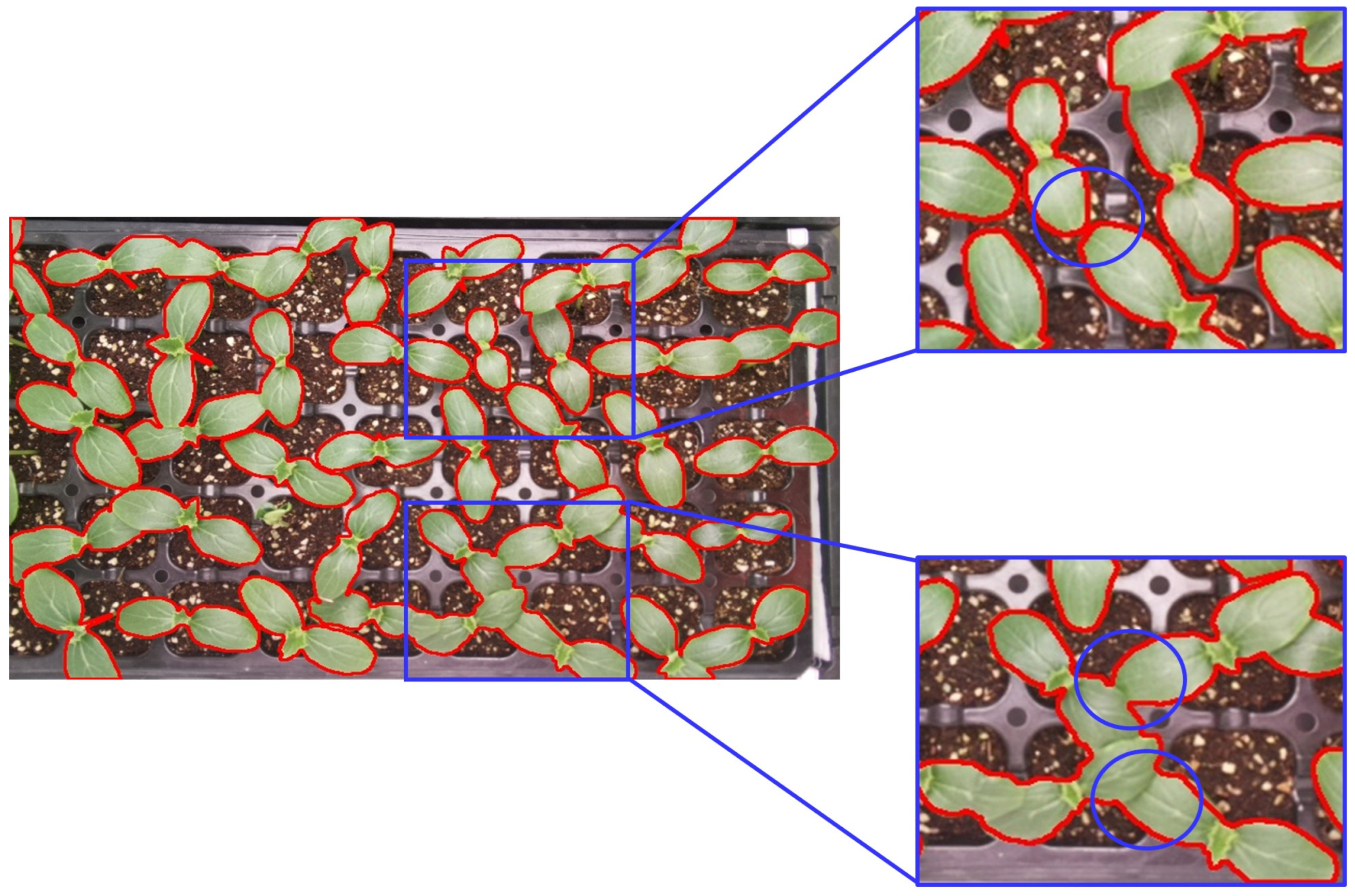
The results indicated that the contour-based annotation method led to faster convergence during training, evidenced by less final training loss (0.50 compared to 0.55 for manual annotation). Additionally, the contour-based method achieved a higher mAP, with an mAP50 of 0.80 and an mAP50-95 of 0.68 compared to 0.78 and 0.65, respectively, for the manually annotated dataset. Although both the methods performed well, manual annotation exhibited marginally higher precision at 0.83 compared to 0.82 for the contour-based approach, indicating its slight advantage in certain aspects of object detection. As shown in Figure 24, the comparison of training and validation losses underscores the efficiency of the contour-based method, while Figure 25 demonstrates the precision–recall curves, where contour-based annotation achieved 98.5% precision and 98.0% recall at an IoU threshold of 0.50 compared to 96% for the manually annotated dataset. The test results are shown in Figure 26, further validating the contour-based approach, with a high overall accuracy ranging from 96% to 98%. Contour determination was crucial for smooth contours, aiding in identifying the exact concave points to reduce the overlap between two leaves of the object, as shown in Figure 27.
However, in regions with lots of vegetation and no gradients, the method tends to draw the contour around the entire seedling (two or three leaves) instead of a single leaf, as shown in Figure 27. Although two adjacent leaves may overlap, precise contour drawing helps detect the exact seedling for further analysis, such as disease and stress detection. This precision also assists in navigating the right position for the precise dosing of nutrients or pesticides, ensuring a targeted and efficient treatment.
The polynomial kernel SVM with five-fold cross-validation combined with contour optimization demonstrated a superior performance in seedling segmentation, surpassing those of the other kernel variations. Optimal feature selection and parameter tuning further enhanced the accuracy. This method also offers a solution to tedious manual annotation through automated contour-based annotation, improving efficiency and precision. Future research could explore alternative machine learning models, improve overlap image segmentation through concave point analysis and apply this approach in real-world environments for real-time monitoring and precision agriculture.

5. Conclusions

This study presented the color and texture features with the SVM to segment the seedlings under different lighting conditions. The main objective was to improve contour preservation and create accurate annotation files for future model training. The setup for the experiment included growing seedlings that were one-week-old in conditions with controlled lighting (50, 250, or 450 μmol·m−2·s−1) and taking daily pictures using RGB cameras for a period of two weeks. Image processing methods, such as filter bank for noise removal and histogram equalization, were utilized to increase the image quality for feature extraction, as well as remove unwanted shadows or color variation from the images, which was evaluated by PSNR and SSIM analyses. In this process, eighteen color features and six texture features were extracted using the GLCM. SFS was used for essential feature selection, and for dimension reduction, PCA was applied. The segmentation of overlapping leaves was addressed by focusing on the concave points of the seedlings. Finally, the SVM was used for seedling object segmentation, while preserving the delicate contour area. The results found that overall segmentation accuracy increased considerably with feature selection, from 73% to 98% for the pepper, 87% to 98% for the tomato, 82% to 97% for the cucumber, and 81% to 98% for the watermelon. The evaluation of the model was performed with a classification report and a confusion matrix, showing minimal misclassification rates ranging from 0.011 to 0.019. Additionally, the annotation files generated were tested in model development, particularly within the YOLOv8 framework. The results showed that these contour-based annotation files achieved high precision (98.5%) and recall (98%) rates, while manual annotation was outperformed slightly in precision (96%) and recall (96%). This confirmed the model’s capability to detect seedlings, with confidence levels ranging from 50% to 98% for both the annotation methods. In conclusion, the proposed method for object segmentation and detection based on the creation of annotation files significantly aided in detecting the seedlings and assessing their health. This approach not only improved segmentation accuracy, but also reduced the human effort required to prepare annotation files for model development. Future studies might investigate other machine learning models, enhance overlap picture segmentation using concave point analysis, and use this strategy in practical settings for precision farming and real-time monitoring.

Author Contributions

Conceptualization, S. and S.-O.C.; methodology, S., M.N.R. and S.-O.C.; software, S., M.N.R. and K.-H.L.; validation, S., M.N.R., S.I., K.-H.L., M.A.H., M.R.A., Y.J.C. and D.H.N.; formal analysis, S., M.N.R., K.-H.L., S.I., M.A.H. and M.R.A.; investigation, Y.J.C., D.H.N. and S.-O.C.; resources, S.-O.C.; data curation, S., M.N.R., K.-H.L., S.I., M.A.H., M.R.A. and Y.J.C.; writing—original draft preparation, S.; writing—review and editing, S., M.N.R., Y.J.C., D.H.N. and S.-O.C.; visualization, S., S.I., M.A.H., M.R.A., Y.J.C. and D.H.N.; supervision, S.-O.C.; project administration, S.-O.C.; funding acquisition, S.-O.C. All authors have read and agreed to the published version of the manuscript.

Funding

This work was supported by the Korea Institute of Planning and Evaluation for Technology in Food, Agriculture and Forestry (IPET), through the Smart Farm Innovation Technology Development Program, funded by the Ministry of Agriculture, Food and Rural Affairs (MAFRA) (Project No. RS-2021-IP421035), Republic of Korea.

Data Availability Statement

The data are contained within this article.

Conflicts of Interest

The authors declare no conflicts of interest.

References

  1. Geng, T.; Yu, H.; Yuan, X.; Ma, R.; Li, P. Research on Segmentation Method of Maize Seedling Plant Instances Based on UAV Multispectral Remote Sensing Images. Plants 2024, 13, 1842. [Google Scholar] [CrossRef] [PubMed]
  2. Tian, H.; Wang, T.; Liu, Y.; Qiao, X.; Li, Y. Computer Vision Technology in Agricultural Automation—A Review. Inf. Process. Agric. 2020, 7, 1–19. [Google Scholar] [CrossRef]
  3. Gupta, M.K.; Samuel, D.V.K.; Sirohi, N.P.S. Decision Support System for Greenhouse Seedling Production. Comput. Electron. Agric. 2010, 73, 133–145. [Google Scholar] [CrossRef]
  4. Ahmed, H.A.; Tong, Y.-X.; Yang, Q.C. Optimal Control of Environmental Conditions Affecting Lettuce Plant Growth in a Controlled Environment with Artificial Lighting: A Review. S. Afr. J. Bot. 2020, 130, 75–89. [Google Scholar] [CrossRef]
  5. Proietti, S.; Moscatello, S.; Riccio, F.; Downey, P.; Battistelli, A. Continuous Lighting Promotes Plant Growth, Light Conversion Efficiency, and Nutritional Quality of Eruca vesicaria (L.) Cav. in Controlled Environment with Minor Effects Due to Light Quality. Front. Plant Sci. 2021, 12, 730119. [Google Scholar] [CrossRef]
  6. Goto, E. Effects of Light Quality on Growth of Crop Plants under Artificial Lighting. Environ. Control Biol. 2003, 41, 121–132. [Google Scholar] [CrossRef]
  7. Islam, S.; Reza, M.N.; Ahmed, S.; Samsuzzaman; Cho, Y.J.; Noh, D.H.; Chung, S.O. Image Processing and Support Vector Machine (SVM) for Classifying Environmental Stress Symptoms of Pepper Seedlings Grown in a Plant Factory. Agronomy 2024, 14, 2043. [Google Scholar] [CrossRef]
  8. Blessing, E. Utilizing Deep Learning, Computer Vision, and Robotics for Crop Monitoring without Human Intervention: Showcasing Advancements like PATHoBot. February 2024. Available online: https://www.researchgate.net/publication/378498623 (accessed on 8 October 2024).
  9. Ruby, E.D.K.; Amirthayogam, G.; Sasi, G.; Chitra, T.; Choubey, A.; Gopalakrishnan, S. Advanced Image Processing Techniques for Automated Detection of Healthy and Infected Leaves in Agricultural Systems. Mesopotamian J. Comput. Sci. 2024, 2024, 62–70. [Google Scholar] [CrossRef]
  10. Lee, D.Y.; Na, D.Y.; Góngora-Canul, C.; Baireddy, S.; Lane, B.; Cruz, A.P.; Fernández-Campos, M.; Kleczewski, N.M.; Telenko, D.E.P.; Goodwin, S.B.; et al. Contour-Based Detection and Quantification of Tar Spot Stromata Using Red-Green-Blue (RGB) Imagery. Front. Plant Sci. 2021, 12, 675975. [Google Scholar] [CrossRef]
  11. Arbeláez, P.; Maire, M.; Fowlkes, C.; Malik, J. Contour Detection and Hierarchical Image Segmentation. IEEE Trans. Pattern Anal. Mach. Intell. 2011, 33, 898–916. [Google Scholar] [CrossRef]
  12. Gwo, C.; Wei, C. Plant Identification through Images: Using Feature Extraction of Key Points on Leaf Contours. Appl. Plant Sci. 2013, 1, 1200005. [Google Scholar] [CrossRef] [PubMed]
  13. Desclaux, D.; Huynh, T.T.; Roumet, P. Identification of Soybean Plant Characteristics That Indicate the Timing of Drought Stress. Crop Sci. 2000, 40, 716–722. [Google Scholar] [CrossRef]
  14. Zhuang, M.; Chen, Z.; Wang, H.; Tang, H.; He, J.; Qin, B.; Yang, Y.; Jin, X.; Yu, M.; Jin, B.; et al. Efficient Contour-Based Annotation by Iterative Deep Learning for Organ Segmentation from Volumetric Medical Images. Int. J. Comput. Assist. Radiol. Surg. 2023, 18, 379–394. [Google Scholar] [CrossRef] [PubMed]
  15. Ahmed, N.; Zhang, B.; Deng, L.; Bozdar, B.; Li, J.; Chachar, S.; Chachar, Z.; Jahan, I.; Talpur, A.; Gishkori, M.S.; et al. Advancing Horizons in Vegetable Cultivation: A Journey from Age-Old Practices to High-Tech Greenhouse Cultivation—A Review. Front. Plant Sci. 2024, 15, 1357153. [Google Scholar] [CrossRef]
  16. Shamshiri, R.R.; Kalantari, F.; Ting, K.C.; Thorp, K.R.; Hameed, I.A.; Weltzien, C.; Ahmad, D.; Shad, Z. Advances in Greenhouse Automation and Controlled Environment Agriculture: A Transition to Plant Factories and Urban Agriculture. Int. J. Agric. Biol. Eng. 2018, 11, 1–22. [Google Scholar] [CrossRef]
  17. Chowdhury, M.; Reza, M.N.; Jin, H.; Islam, S.; Lee, G.J.; Chung, S.O. Defective Pennywort Leaf Detection Using Machine Vision and Mask R-CNN Model. Agronomy 2024, 14, 2313. [Google Scholar] [CrossRef]
  18. Wang, Q.; Du, W.; Ma, C.; Gu, Z. Gradient Color Leaf Image Segmentation Algorithm Based on Meanshift and Kmeans. In Proceedings of the 2021 IEEE 5th Advanced Information Technology, Electronic and Automation Control Conference (IAEAC), Chongqing, China, 12–14 March 2021; pp. 1609–1614. [Google Scholar] [CrossRef]
  19. Li, M.; Liao, J.J. Texture Image Segmentation Based on GLCM. Appl. Mech. Mater. 2012, 220–223, 1398–1401. [Google Scholar] [CrossRef]
  20. Samiei, S.; Rasti, P.; Vu, J.L.; Buitink, J.; Rousseau, D. Deep Learning-Based Detection of Seedling Development. Plant Methods 2020, 16, 103. [Google Scholar] [CrossRef]
  21. Hsu, R.C.; Chan, D.Y.; Liu, C.T.; Lai, W.C. Contour Extraction in Medical Images Using Initial Boundary Pixel Selection and Segmental Contour Following. Multidimens. Syst. Signal Process. 2012, 23, 469–498. [Google Scholar] [CrossRef]
  22. Yang, X.; Chen, A.; Zhou, G.; Wang, J.; Chen, W.; Gao, Y.; Jiang, R. Instance Segmentation and Classification Method for Plant Leaf Images Based on ISC-MRCNN and APS-DCCNN. IEEE Access 2020, 8, 151555–151573. [Google Scholar] [CrossRef]
  23. Oudah, M.; Al-Naji, A.; AL-Janabi, T.Y.; Namaa, D.S.; Chahl, J. Automatic Irrigation System Based on Computer Vision and an Artificial Intelligence Technique Using Raspberry Pi. Automation 2024, 5, 90–105. [Google Scholar] [CrossRef]
  24. Gai, J.; Tang, L.; Steward, B.L. Automated Crop Plant Detection Based on the Fusion of Color and Depth Images for Robotic Weed Control. J. Field Robot. 2020, 37, 35–52. [Google Scholar] [CrossRef]
  25. Sanou, I.W.; Baderot, J.; Bricq, S.; Benezeth, Y.; Marzani, F.; Martinez, S.; Foucher, J. Deep Learning Contour-Based Method for Semi-Automatic Annotation of Manufactured Objects in Electron Microscopy Images. J. Electron. Imaging 2024, 33, 031204. [Google Scholar] [CrossRef]
  26. Jasim, W.N.; Mohammed, R.J. A Survey on Segmentation Techniques for Image Processing. Iraqi J. Electr. Electron. Eng. 2021, 17, 73–93. [Google Scholar] [CrossRef]
  27. Kurugollu, F.; Sankur, B.; Harmanci, A.E. Color Image Segmentation Using Histogram Multithresholding and Fusion. Image Vis. Comput. 2001, 19, 915–928. [Google Scholar] [CrossRef]
  28. Muntarina, K.; Shorif, S.B.; Uddin, M.S. Notes on Edge Detection Approaches. Evol. Syst. 2022, 13, 169–182. [Google Scholar] [CrossRef]
  29. Xu, X.; Qiu, J.; Zhang, W.; Zhou, Z.; Kang, Y. Soybean Seedling Root Segmentation Using Improved U-Net Network. Sensors 2022, 22, 8904. [Google Scholar] [CrossRef]
  30. Sun, S.; Zhu, Y.; Liu, S.; Chen, Y.; Zhang, Y.; Li, S. An Integrated Method for Phenotypic Analysis of Wheat Based on Multi-View Image Sequences: From Seedling to Grain Filling Stages. Front. Plant Sci. 2024, 15, 1459968. [Google Scholar] [CrossRef]
  31. Wu, Y.; He, Y.; Wang, Y. Multi-Class Weed Recognition Using Hybrid CNN-SVM Classifier. Sensors 2023, 23, 7153. [Google Scholar] [CrossRef]
  32. Kumar, A.; Sachar, S. Deep Learning Techniques in Leaf Image Segmentation and Leaf Species Classification: A Survey. Wireless Pers. Commun. 2023, 133, 2379–2410. [Google Scholar] [CrossRef]
  33. Wang, S.; Li, C.; Wang, R.; Liu, Z.; Wang, M.; Tan, H.; Wu, Y.; Liu, X.; Sun, H.; Yang, R.; et al. Annotation-Efficient Deep Learning for Automatic Medical Image Segmentation. Nat. Commun. 2021, 12, 5915. [Google Scholar] [CrossRef] [PubMed]
  34. Thompson, N.; Greenewald, K.; Lee, K.; Manso, G.F. The Computational Limits of Deep Learning. arXiv 2021, arXiv:2007.05558. [Google Scholar]
  35. Kiss, A.; Moreau, T.; Mirabet, V.; Calugaru, C.I.; Boudaoud, A.; Das, P. Segmentation of 3D Images of Plant Tissues at Multiple Scales Using the Level Set Method. Plant Methods 2017, 13, 114. [Google Scholar] [CrossRef] [PubMed]
  36. Narisetti, N.; Henke, M.; Neumann, K.; Stolzenburg, F.; Altmann, T.; Gladilin, E. Deep Learning Based Greenhouse Image Segmentation and Shoot Phenotyping (DeepShoot). Front. Plant Sci. 2022, 13, 906410. [Google Scholar] [CrossRef]
  37. Yang, A.; Bai, Y.; Liu, H.; Jin, K.; Xue, T.; Ma, W. Application of SVM and Its Improved Model in Image Segmentation. Mob. Netw. Appl. 2022, 27, 851–861. [Google Scholar] [CrossRef]
  38. Attri, I.; Awasthi, L.K.; Sharma, T.P.; Rathee, P. A Review of Deep Learning Techniques Used in Agriculture. Ecol. Inform. 2023, 77, 102217. [Google Scholar] [CrossRef]
  39. Li, M.; Yu, X.; Ryu, K.H.; Lee, S.; Theera-Umpon, N. Face Recognition Technology Development with Gabor, PCA and SVM Methodology under Illumination Normalization Condition. Cluster Comput. 2018, 21, 1117–1126. [Google Scholar] [CrossRef]
  40. Islam, S.; Reza, M.N.; Ahmed, S.; Samsuzzaman; Cho, Y.J.; Noh, D.H.; Chung, S.O. Seedling Growth Stress Quantification Based on Environmental Factors Using Sensor Fusion and Image Processing. Horticulturae 2024, 10, 186. [Google Scholar] [CrossRef]
  41. Feng, L.; Raza, M.A.; Li, Z.; Chen, Y.; Khalid, M.H.B.; Du, J.; Liu, W.; Wu, X.; Song, C.; Yu, L.; et al. The Influence of Light Intensity and Leaf Movement on Photosynthesis Characteristics and Carbon Balance of Soybean. Front. Plant Sci. 2019, 9, 1952. [Google Scholar] [CrossRef]
  42. Javidan, S.M.; Banakar, A.; Rahnama, K.; Vakilian, K.A.; Ampatzidis, Y. Feature Engineering to Identify Plant Diseases Using Image Processing and Artificial Intelligence: A Comprehensive Review. Smart Agric. Technol. 2024, 8, 100480. [Google Scholar] [CrossRef]
  43. Yalman, Y. A Histogram Based Image Quality Index. Prz. Elektrotech. 2012, 88, 126–129. [Google Scholar]
  44. Guo, J.; Ma, J.; García-Fernández, Á.F.; Zhang, Y.; Liang, H. A Survey on Image Enhancement for Low-Light Images. Heliyon 2023, 9, e14558. [Google Scholar] [CrossRef] [PubMed]
  45. Pizer, S.M.; Amburn, E.P.; Austin, J.D.; Cromartie, R.; Geselowitz, A.; Greer, T.; Haar Romeny, B.t.; Zimmerman, J.B.; Zuiderveld, K. Adaptive Histogram Equalization and Its Variations. Comput. Vis. Graph. Image Process. 1987, 39, 355–368. [Google Scholar] [CrossRef]
  46. Dhal, K.G.; Das, A.; Ray, S.; Gálvez, J.; Das, S. Histogram Equalization Variants as Optimization Problems: A Review. Arch. Comput. Methods Eng. 2021, 28, 1471–1496. [Google Scholar] [CrossRef]
  47. Sepasian, M.; Balachandran, W.; Mares, C. Image Enhancement for Fingerprint Minutiae-Based Algorithms Using CLAHE, Standard Deviation Analysis and Sliding Neighborhood. Lect. Notes Eng. Comput. Sci. 2008, 2173, 1199–1203. Available online: https://www.researchgate.net/publication/44262481 (accessed on 5 October 2024).
  48. Azam, M.; Nouman, M. Evaluation of Image Support Resolution Deep Learning Technique Based on PSNR Value. KIET J. Comput. Inf. Sci. 2022, 6, 93–122. [Google Scholar] [CrossRef]
  49. Sridhar, S.; Kumar, P.R.; Ramanaiah, K.V. Wavelet Transform Techniques for Image Compression—An Evaluation. Int. J. Image Graph. Signal Process. 2014, 6, 54–67. [Google Scholar] [CrossRef]
  50. Sara, U.; Akter, M.; Uddin, M.S. Image Quality Assessment through FSIM, SSIM, MSE and PSNR—A Comparative Study. J. Comput. Commun. 2019, 7, 8–18. [Google Scholar] [CrossRef]
  51. Wang, Z.; Bovik, A.C.; Sheikh, H.R.; Simoncelli, E.P. Image Quality Assessment: From Error Visibility to Structural Similarity. IEEE Trans. Image Process. 2004, 13, 600–612. [Google Scholar] [CrossRef]
  52. Yuan, W.; Wijewardane, N.K.; Jenkins, S.; Bai, G.; Ge, Y.; Graef, G.L. Early Prediction of Soybean Traits through Color and Texture Features of Canopy RGB Imagery. Sci. Rep. 2019, 9, 14089. [Google Scholar] [CrossRef]
  53. Yue, J.; Li, Z.; Liu, L.; Fu, Z. Content-Based Image Retrieval Using Color and Texture Fused Features. Math. Comput. Model. 2011, 54, 1121–1127. [Google Scholar] [CrossRef]
  54. Shrivastava, V.K.; Pradhan, M.K. Rice Plant Disease Classification Using Color Features: A Machine Learning Paradigm. J. Plant Pathol. 2021, 103, 17–26. [Google Scholar] [CrossRef]
  55. Hu, X.; Ensor, A. Fourier Spectrum Image Texture Analysis. In Proceedings of the 2018 International Conference on Image and Vision Computing New Zealand (IVCNZ), Auckland, New Zealand, 19–21 November 2018; pp. 1–6. [Google Scholar] [CrossRef]
  56. Szczypiński, P.M.; Strzelecki, M.; Materka, A.; Klepaczko, A. MaZda-A Software Package for Image Texture Analysis. Comput. Methods Programs Biomed. 2009, 94, 66–76. [Google Scholar] [CrossRef] [PubMed]
  57. Zubair, A.R.; Alo, O.A. Grey Level Co-Occurrence Matrix (GLCM) Based Second Order Statistics for Image Texture Analysis. Int. J. Sci. Eng. Investig. 2019, 8, 93. Available online: www.IJSEI.com (accessed on 3 September 2024).
  58. Yao, Q.; Guan, Z.; Zhou, Y.; Tang, J.; Hu, Y.; Yang, B. Application of Support Vector Machine for Detecting Rice Diseases Using Shape and Color Texture Features. In Proceedings of the 2009 International Conference on Engineering Computation, Hong Kong, China, 2–3 May 2009; pp. 79–83. [Google Scholar] [CrossRef]
  59. Nadafzadeh, M.; Abdanan Mehdizadeh, S. Design and Fabrication of an Intelligent Control System for Determination of Watering Time for Turfgrass Plant Using Computer Vision System and Artificial Neural Network. Precis. Agric. 2019, 20, 857–879. [Google Scholar] [CrossRef]
  60. Cai, J.; Luo, J.; Wang, S.; Yang, S. Feature Selection in Machine Learning: A New Perspective. Neurocomputing 2018, 300, 70–79. [Google Scholar] [CrossRef]
  61. Al-Tashi, Q.; Abdulkadir, S.J.; Rais, H.M.; Mirjalili, S.; Alhussian, H. Approaches to Multi-Objective Feature Selection: A Systematic Literature Review. IEEE Access 2020, 8, 125076–125096. [Google Scholar] [CrossRef]
  62. Aggrawal, R.; Pal, S. Sequential Feature Selection and Machine Learning Algorithm-Based Patient’s Death Events Prediction and Diagnosis in Heart Disease. SN Comput. Sci. 2020, 1, 344. [Google Scholar] [CrossRef]
  63. Rückstieß, T.; Osendorfer, C.; Van Der Smagt, P. Sequential Feature Selection for Classification; Springer: Berlin/Heidelberg, Germany, 2011; pp. 132–141. [Google Scholar] [CrossRef]
  64. Dubey, S.R.; Dixit, P.; Singh, N.; Gupta, J.P. Infected Fruit Part Detection Using K-Means Clustering Segmentation Technique. Int. J. Interact. Multimed. Artif. Intell. 2013, 2, 65. [Google Scholar] [CrossRef]
  65. Soliman, O.S.; Mahmoud, A.S. A Classification System for Remote Sensing Satellite Images Using Support Vector Machine with Non-Linear Kernel Functions. In Proceedings of the 2012 8th International Conference on Informatics and Systems (INFOS), Giza, Egypt, 14–16 May 2012. [Google Scholar]
  66. Hussain, M.; Wajid, S.K.; Elzaart, A.; Berbar, M. A Comparison of SVM Kernel Functions for Breast Cancer Detection. In Proceedings of the 2011 Eighth International Conference Computer Graphics, Imaging and Visualization, Singapore, 17–19 August 2011; pp. 145–150. [Google Scholar] [CrossRef]
  67. Wang, Z. Cell Segmentation for Image Cytometry: Advances, Insufficiencies, and Challenges. Cytom. Part A 2019, 95, 708–711. [Google Scholar] [CrossRef]
  68. Vădineanu, Ş.; Pelt, D.M.; Dzyubachyk, O.; Batenburg, K.J. Reducing Manual Annotation Costs for Cell Segmentation by Upgrading Low-Quality Annotations; Springer: Cham, Switzerland, 2023; pp. 3–13. [Google Scholar] [CrossRef]
  69. Lu, Y.; Zheng, K.; Li, W.; Wang, Y.; Harrison, A.P.; Lin, C.; Wang, S.; Xiao, J.; Lu, L.; Kuo, C.F.; et al. Contour Transformer Network for One-Shot Segmentation of Anatomical Structures. IEEE Trans. Med. Imaging 2021, 40, 2672–2684. [Google Scholar] [CrossRef] [PubMed]
  70. Tatsumi, K.; Tanino, T. Support Vector Machines Maximizing Geometric Margins for Multi-Class Classification. Top 2014, 22, 815–840. [Google Scholar] [CrossRef]
  71. Montesinos López, O.A.; Montesinos López, A.; Crossa, J. Overfitting, Model Tuning, and Evaluation of Prediction Performance; Springer: Cham, Switzerland, 2022. [Google Scholar] [CrossRef]
  72. Santos, M.S.; Soares, J.P.; Abreu, P.H.; Araujo, H.; Santos, J. Cross-Validation for Imbalanced Datasets: Avoiding Overoptimistic and Overfitting Approaches. IEEE Comput. Intell. Mag. 2018, 13, 59–76. [Google Scholar] [CrossRef]
  73. Hashemzadeh, K.; Hashemzadeh, S. Maximum Relative Margin and Data-Dependent Regularization Pannagadatta. Minerva Chir. 2012, 67, 327–335. [Google Scholar]
  74. Xue, H.; Chen, S.; Yang, Q. Discriminatively Regularized Least-Squares Classification. Pattern Recognit. 2009, 42, 93–104. [Google Scholar] [CrossRef]
  75. Wang, C.; Deng, C.; Yu, Z.; Hui, D.; Gong, X.; Luo, R. Adaptive Ensemble of Classifiers with Regularization for Imbalanced Data Classification. Inf. Fusion 2021, 69, 81–102. [Google Scholar] [CrossRef]
  76. Guo, Z.; Hu, X.; Zhao, B.; Wang, H.; Ma, X. StrawSnake: A Real-Time Strawberry Instance Segmentation Network Based on the Contour Learning Approach. Electronics 2024, 13, 3103. [Google Scholar] [CrossRef]
  77. Gao, L.; Lin, X. A Method for Accurately Segmenting Images of Medicinal Plant Leaves with Complex Backgrounds. Comput. Electron. Agric. 2018, 155, 426–445. [Google Scholar] [CrossRef]
  78. Sadeghi-Tehran, P.; Virlet, N.; Sabermanesh, K.; Hawkesford, M.J. Multi-Feature Machine Learning Model for Automatic Segmentation of Green Fractional Vegetation Cover for High-Throughput Field Phenotyping. Plant Methods 2017, 13, 103. [Google Scholar] [CrossRef]
  79. Ghosh, S.; Singh, A.; Kavita; Jhanjhi, N.Z.; Masud, M.; Aljahdali, S. SVM and KNN Based CNN Architectures for Plant Classification. Comput. Mater. Contin. 2022, 71, 4257–4274. [Google Scholar] [CrossRef]
  80. Hossain, E.; Hossain, M.F.; Rahaman, M.A. A Color and Texture-Based Approach for the Detection and Classification of Plant Leaf Disease Using KNN Classifier. In Proceedings of the 2019 International Conference on Electrical, Computer and Communication Engineering (ECCE), Cox’s Bazar, Bangladesh, 7–9 February 2019; pp. 1–6. [Google Scholar] [CrossRef]
  81. Zhang, S.; Wang, H.; Huang, W.; You, Z. Plant Diseased Leaf Segmentation and Recognition by Fusion of Superpixel, K-Means, and PHOG. Optik 2018, 157, 866–872. [Google Scholar] [CrossRef]
  82. Wang, W.; Chen, Z.; Yuan, X.; Wu, X. Adaptive Image Enhancement Method for Correcting Low-Illumination Images. Inf. Sci. 2019, 496, 25–41. [Google Scholar] [CrossRef]
  83. Ijaz, E.D.U.; Ijaz, E.A.; Ali Iqbal, D.F.G.; Hayat, M. Quantitative Analysis of Image Enhancement Algorithms for Diverse Applications. Int. J. Innov. Sci. Technol. 2023, 5, 694–707. [Google Scholar]
  84. Juneja, M.; Saini, S.K.; Gupta, J.; Garg, P.; Thakur, N.; Sharma, A.; Mehta, M.; Jindal, P. Survey of Denoising, Segmentation and Classification of Magnetic Resonance Imaging for Prostate Cancer. Multimed. Tools Appl. 2021, 80, 29199–29249. [Google Scholar] [CrossRef]
  85. Büyükarıkan, B.; Ülker, E. Convolutional Neural Network-Based Apple Images Classification and Image Quality Measurement by Light Colors Using the Color-Balancing Approach. Multimed. Syst. 2023, 29, 1651–1661. [Google Scholar] [CrossRef]
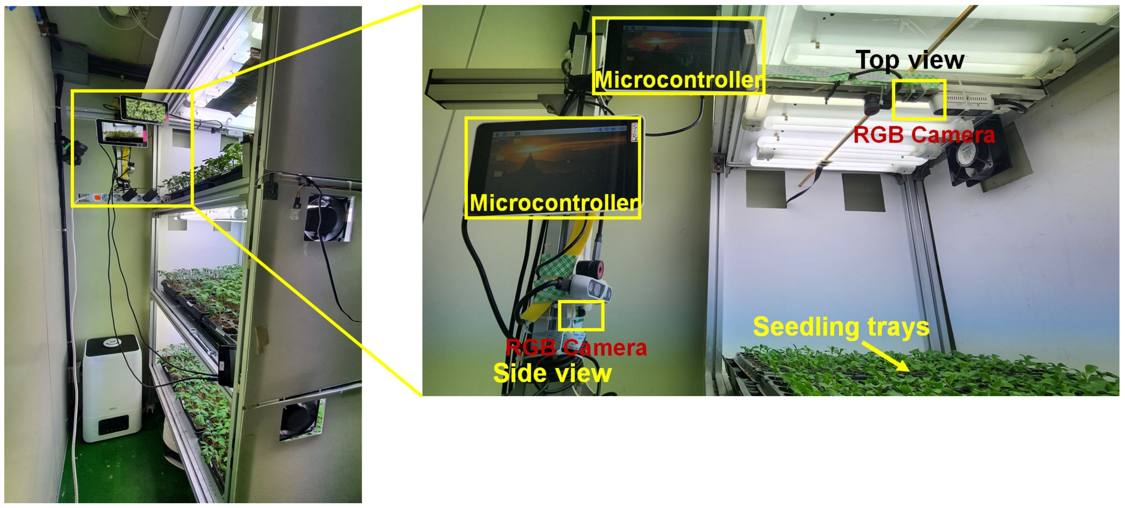
Figure 1. Image acquisition from top and side views using commercial camera setup for four types of seedlings in controlled plant factory chamber.
Agronomy 14 02940 g001
Figure 2. Vertical section of seedling growing chamber designed to maintain different light intensities for each plant bed: (a) plant beds arranged in separate layers, and (b) lighting arrangement for each bed to achieve specific light conditions.
Agronomy 14 02940 g002
Figure 3. Images of seedlings grown in plant factory: (a) tomato, (b) cucumber, (c) pepper, (d) watermelon. (e) Various background elements in images, including seedling, soil, and seedling tray.
Agronomy 14 02940 g003
Figure 4. Overall image preprocessing steps and feature extraction and seedling segmentation process used in this study.
Agronomy 14 02940 g004
Figure 5. Image preprocessing workflow includes noise removal, contrast enhancement with histogram equalization, and quality assessment using PSNR and SSIM metrics: (a) original image with histogram, (b) noise-removed and histogram-equalized image, and (c) optimum clip limit selection for accurate histogram equalization using PSNR and SSIM analysis.
Agronomy 14 02940 g005
Figure 6. Six color spaces were used from all seedling images in this study: (a) RGB, (b) HSV, (c) XYZ, (d) YUV, (e) YCbCr, and (f) LAB.
Agronomy 14 02940 g006
Figure 7. Schematic diagram for seedling texture feature extraction process.
Agronomy 14 02940 g007
Figure 8. Texture feature analysis using GLCM method: (a) homogeneity, (b) contrast, (c) correlation, (d) energy, and (e) entropy.
Agronomy 14 02940 g008
Figure 9. (a) Three-dimensional visualization of data patterns under different environmental lighting conditions (50, 250, and 450 µmol·m⁻2·s⁻1), where the red circles indicate seedlings and the blue circles indicate the background, and (b) hierarchical clustering dendrogram for data points based on 18 color features and 6 texture features.
Agronomy 14 02940 g009
Figure 10. Schematic diagram of SFS method to select features used in this study.
Agronomy 14 02940 g010
Figure 11. Illustration of SVM optimal hyperplane, margin, and support vectors for linearly separable dataset. Dark blue and light blue circles represent Class A and Class B data points, respectively.
Agronomy 14 02940 g011
Figure 12. SVM segmentation model development in this study.
Agronomy 14 02940 g012
Figure 13. Images for segmentation model development and pixels of seedlings, soil, and tray. Dark blue circles represent seedling area, while pink circles highlight seedling image background. (a) tomato, (b) cucumber, (c) pepper, and (d) watermelon.
Agronomy 14 02940 g013
Figure 14. Working flow diagram for image segmentation using color transformation and feature extraction. Red circles represent seedlings, while blue circles represent the background. The segmentation process is performed using SVM in this study.
Agronomy 14 02940 g014
Figure 15. Flow diagram of annotation file preparation from the contour image dataset for real-time seedling detection model. (1–5) represent the unique class of objects.
Agronomy 14 02940 g015
Figure 16. Feature selection performance curve using SFS method (selected features are indicated by red, dashed lines).
Agronomy 14 02940 g016
Figure 17. Impact of SFS on SVM classification performance for seedling (white dots) and background segmentation (black dots): (a) decision boundary without SFS methods achieving 73% accuracy, (b) and decision boundary with SFS, improving accuracy to 98%.
Agronomy 14 02940 g017
Figure 18. Pixel classification using the SVM without feature selection under varying light conditions: (a) 50 µmol·m⁻2·s⁻1, (b) 250 µmol·m⁻2·s⁻1, and (c) 450 µmol·m⁻2·s⁻1. The left panel shows the segmented images with visible noise around the seedlings. The center panel presents pixel classification scatter plots considering all the features, highlighting the clusters of background (red) and seedling (blue) pixels. The right panel displays the resulting contour detection on the segmented images, revealing inaccurate contours and noisy boundaries due to the presence of noise.
Agronomy 14 02940 g018
Figure 19. Segmentation performance of seedling images under different lighting conditions ((a) = 50, (b) = 250, and (c) = 450 µmol·m⁻2·s⁻1). Random colors represent seedling detection of different shapes.
Agronomy 14 02940 g019
Figure 20. Overall classification results using SVM method with different kernels: (a) decision boundaries for linear kernels with 0, 5, and 10-fold cross-validation, C = 0; (b) decision boundaries for RBF kernels with 0, 5, and 10-fold cross-validation, C = 128,100, and γ = 128, 512; and (c) decision boundaries for polynomial kernels with 0, 5, and 10-fold cross-validation, C = 60, and γ = 0, degree = 3. In all figures, seedlings are represented by white circles, and black dots represents background.
Agronomy 14 02940 g020
Figure 21. Segmented masked image, contour, and bounding box detection using various seedling images: (a) pepper, (b) cucumber, (c) tomato, and (d) watermelon.
Agronomy 14 02940 g021
Figure 22. Performance evaluation of SVM model: confusion matrices for (1) pepper, (2) tomato, (3) cucumber, and (4) watermelon: (a) before applying feature section method, (b) confusion metrics after feature selection method, and (c) ROC curve with accuracy of 98%.
Agronomy 14 02940 g022
Figure 23. Correlation between actual ground truth area and segmented canopy area for different seedlings: (a) cucumber, (b) pepper, (c) tomato, and (d) watermelon.
Agronomy 14 02940 g023
Figure 24. Training and validation performance of proposed YOLOv8 model, highlighting various loss functions, box loss (B), mask loss (M), segmentation loss, classification loss, and validation loss, as well as key metrics, including precision, recall, and mAP at IoU thresholds of 0.5 and 0.5–0.95. (a) Results using contour-based annotated dataset, and (b) results using manual annotated dataset.
Agronomy 14 02940 g024
Figure 25. The precision–recall and recall–confidence curves for seedling segmentation: (a) results using contour-based annotation dataset, and (b) results using manual annotated dataset.
Agronomy 14 02940 g025
Figure 26. Test results using YOLOv8 model, trained with contour-based annotation dataset. Model accurately detects seedlings, (a) pepper, (b) cucumber, (c) tomato, and (d) watermelon, with confidence levels ranging from 50% to 98%.
Agronomy 14 02940 g026
Figure 27. Sample images demonstrate separation of overlapped seedling leaves with accurate contour detection for precise seedling identification. Blue circle indicates successful separation of overlapped leaves (top cropped image), and instance where leaves remain connected, with only contour drawn around joined leaf sections (lower cropped image).
Agronomy 14 02940 g027
Table 1. Specifications of microcontroller and camera used in this study.
ParameterMicrocontrollerParameterCamera
NameRaspberry Pi 4B boardNameRaspberry Pi Camera Module 2
CPUQuad-core Cortex-A72, 64-bit, 1.8 GHzSensorSony IMX 219 PQ CMOS
RAM8 GB LPDDR4-3200Resolution8 MP
Operating systemLinux basedFPS108p: 30; 720p: 60
ConnectionStandard 40-pin GPIO headerResolution3280 × 2464 pixel
Power5 V DCConnection15-pin MIPI CSI-2
Operating temperature0 to 50 °CImage controlAutomatic
Table 2. SVM classification performance with and without feature selection using SFS method.
ParameterSVM Classification with the SFS MethodSVM Classification Without the SFS Method
PrecisionRecallF1-ScoreSupportPrecisionRecallF1-ScoreSupport
Seedlings 0.990.980.983010.880.450.60264
Background 0.980.990.982990.690.950.80336
Accuracy 0.98600 0.73600
Macro avg.0.980.980.986000.790.700.70600
Weighted avg.0.980.970.986000.770.730.71600
Table 3. Classification performance of SVM models with linear, polynomial, and RBF kernels under 0, 5, and 10-fold cross-validation using varying regularization parameters (c = 0, 10, 60, 128) and kernel coefficients (γ = 0, 128, 512).
ParameterSVM Classification with Linear KernelSVM Classification with Polynomial KernelSVM Classification with RBF Kernel
PrecisionRecallF1-ScoreSupportPrecisionRecallF1-ScoreSupportPrecisionRecallF1-ScoreSupport
CV-0Seedling 0.930.900.92302960.950.953020.940.910.92302
Background 0.910.940.922980.950.960.952980.920.910.92298
Accuracy 0.81600 0.86600 0.81600
Macro avg.0.800.770.786000.910.810.836000.790.780.79600
Weighted avg.0.800.810.806000.890.860.856000.800.810.8060
CV-5Seedling 0.960.950.963020.990.980.983010.960.950.96302
Background 0.950.960.962980.980.990.982990.950.960.96298
Accuracy 0.96600 0.98600 0.96600
Macro avg.0.960.960.966000.980.980.986000.960.950.96600
Weighted avg.0.960.960.966000.980.970.986000.950.960.96600
CV-10Seedling 0.900.830.873010.920.820.873010.900.840.87301
Background 0.840.910.872990.840.930.892990.850.910.88299
Accuracy 0.87600 0.88600 0.88600
Macro avg.0.870.870.876000.880.880.886000.880.880.87600
Weighted avg.0.870.860.876000.880.880.886000.880.880.87600
Table 4. Performance evaluation of SVM model using mean absolute error between testing and prediction results.
Kernel TypeCVC, γMAEPrecisionRecallF1-ScoreAccuracy
Polynomial5C = 60
γ = 0
Degree = 3
0.270.770.730.7173%
Linear0C = 100.190.800.810.8081%
Linear5C = 100.040.960.960.9696%
Linear10C = 300.130.870.860.8787%
RBF0C = 128
γ = 128
0.190.800.810.8081%
RBF5C = 100
γ = 512
0.040.950.960.9696%
RBF10C = 128
γ = 128
0.130.880.880.8787%
Polynomial0C = 60
γ = 0
Degree = 3
0.140.890.860.8586%
Polynomial5C = 60
γ = 0
Degree = 3
0.020.980.970.9898%
Polynomial10C = 60
γ = 0
Degree = 3
0.120.880.880.8888%
Table 5. Comparative analysis of different segmentation models with model in current study.
ModelSegmentation Accuracy
OTSU + watershed segmentation [77]81%
Multi-feature learning method (MFL) [78]89%
CNN + KNN [79]99%
K nearest neighbor (KNN) [80]91%
K means + PHOG [81]85%
Proposed method98%
Disclaimer/Publisher’s Note: The statements, opinions and data contained in all publications are solely those of the individual author(s) and contributor(s) and not of MDPI and/or the editor(s). MDPI and/or the editor(s) disclaim responsibility for any injury to people or property resulting from any ideas, methods, instructions or products referred to in the content.