Optimization Design and Experimental Analysis of Resistance-Reducing Anti-Fracture Rotary Blade Based on DEM Techniques

Abstract

To address the significant cutting resistance and fracture susceptibility of rotary blades, an innovative blade design was conceived to minimize resistance and enhance fracture resistance. By analyzing the interaction between the blade, soil, and root systems, an optimized design for the blade structure’s breakage resistance was developed. The theory of eccentric circular side cutting edges was applied to redesign the curve of the side cutting edge, and kinematic analysis was conducted to determine the optimal edge angle (26.57°). A flexible body model of corn residues was established, and cutting resistance measurements indicated a 15.1% reduction in cutting resistance. The breakage resistance of the rotary blade was validated using a discrete element method–finite element method (DEM–FEM) coupling approach. The results demonstrated the following: neck stress (−16.85%), specific strength efficiency (+9.72%), specific stiffness efficiency (+9.78%), fatigue life (+39.08%), and ultimate fracture stress (+20.16%), thereby meeting the design objectives. The comparison between field trial results and simulation data showed an error rate (<5%), confirming the simulation test’s feasibility. These findings provide theoretical references for reducing cutting resistance and enhancing breakage resistance in rotary blades.

1. Introduction

Rotary tillage and soil-preparation machines are integral to maintaining the quality and efficiency of China’s 120 million hectares of cultivated land. These machines are essential for the accurate land preparation required in modern agricultural production. The rotary blade, a crucial component, significantly affects the overall machine quality, operational effectiveness, efficiency, and power consumption, thus influencing the extent and level of mechanization in soil preparation. During operation, rotary blades face a complex array of forces, including friction, impact, extrusion, and bending from soil, gravel, hard stones, and plant roots. These conditions often lead to wear, breakage, and failure to meet operational standards [1]. In hilly and mountainous areas, blades frequently encounter obstacles such as clods, rocks, and roots at varying heights due to significant terrain fluctuations. This causes the blade to bear instantaneous high impact load, resulting in greater stress concentration and increasing the likelihood of fracture. In addition, frequent load fluctuations subject the blade to forces from multiple directions in short periods, exacerbating fatigue damage [2]. Incomplete statistics suggest that approximately 30% of rotary blades experience fracture failure during operation. Blade fractures not only reduce operational efficiency and quality but also increase costs, potentially delaying agricultural production and causing casualties. To address this issue, some researchers have developed a soil model that can detect the stress levels at the neck of the rotary blade during tilling operations. They addressed these stress concentrations by designing concave–convex-reinforced ribs and modifying the cross-sectional shape of the blade neck [3]. Other researchers applied damage and fracture mechanics to quantitatively describe crack formation and propagation rates. Utilizing discrete element simulation and stress intensity factor correction, they verified the crack propagation patterns of the rotary blade under normal cyclic and impact overload conditions [4].

To enhance the working efficiency of rotary tillers, numerous researchers have explored means to optimize the geometric structure of rotary blades. Agricultural engineering has embraced biomimicry, for instance, in the design of a bionic rotary blade inspired by the multi-toe structure of moles. Studies have demonstrated that this design reduced the blade’s overall power consumption by approximately 20% across a range of forward and rotational speeds [5]. Similarly, a bionic blade tooth modeled after a badger’s claw structure exhibited an average power consumption reduction of 0.08 kW compared to conventional teeth while also decreasing soil adhesion by 84.29% [6]. In addition, a wedge-shaped rotary blade, created through structural parameter modifications, has demonstrated the ability to reduce cutting resistance by 11.35% [7]. While these analyses have primarily focused on optimizing rotary blade structures to minimize resistance and energy consumption, there remains a dearth of research aimed at enhancing fracture resistance through structural design.

The discrete element method (DEM) has been extensively employed to appraise the interactions between soil, components, and machinery [8,9]. Current model development and simulation analyses primarily center on equipment such as crushers [10,11], deep loosening machines [12,13], and rotary tillers [14,15]. These studies are generally classified into two main categories, depending on their research objectives. One approach involves researchers utilizing existing DEM data to optimize the geometric structure of cutting tools. This method focuses on optimizing the edge curvature and sliding angle of rotary blades to evaluate their impact on soil disturbance characteristics, followed by adjustments to the blade body parameters [16]. The alternative approach involves the calibration of soil, straw, crops, and other elements, such as the modeling and calibration of corn stubble. This method allows for a more accurate simulation of shear and cutting processes during operation, thereby enhancing the reliability of discrete element simulation [17].

This paper introduces a structurally optimized design for a novel rotary blade that effectively minimizes resistance and improves fracture resistance. While maintaining the conventional straight cutting edge and transition section, the design reimagines the blade body and handle. To verify the cutting performance of the newly designed blade, a composite model of corn residues and soil was developed utilizing the discrete element method. Additionally, the blade’s fracture resistance was evaluated through a DEM–FEM coupling approach. The results demonstrate that this design significantly enhances the fracture resistance and longevity of the rotary blade on the basis of having an excellent cutting performance. This innovative blade has been designated as the RA rotary blade.

2. Materials and Methods

2.1. Design of the Side Cutting-Edge Curve of the RA Rotary Blade

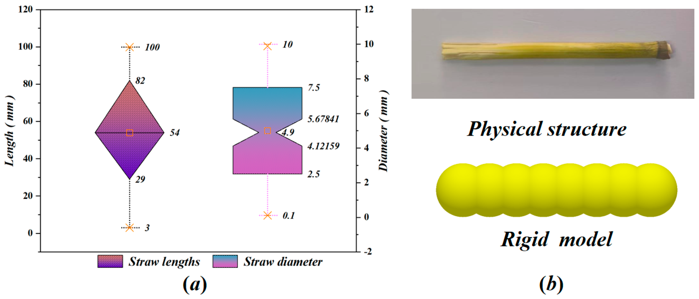
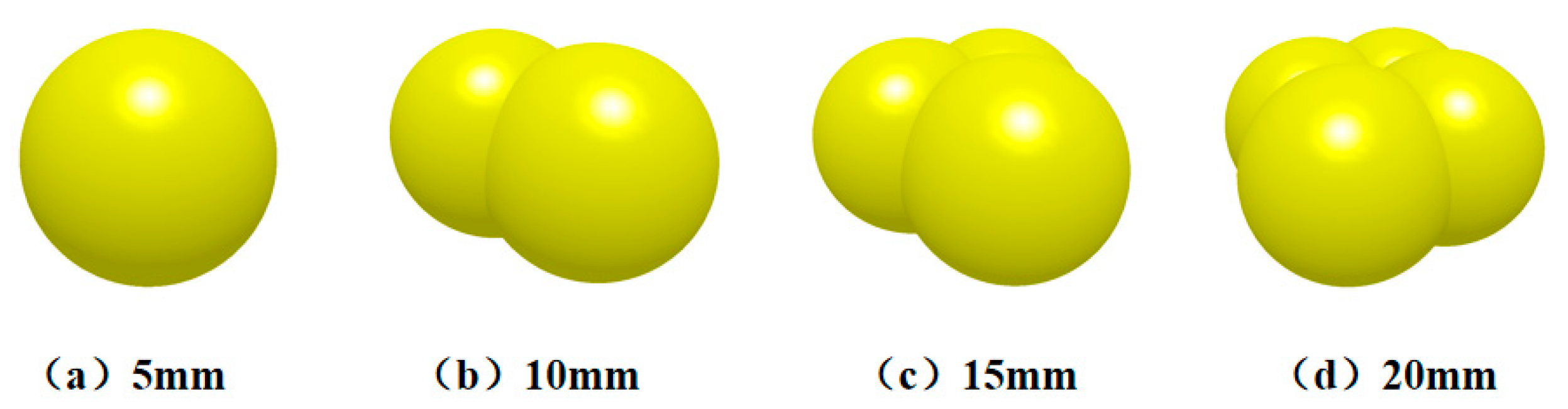
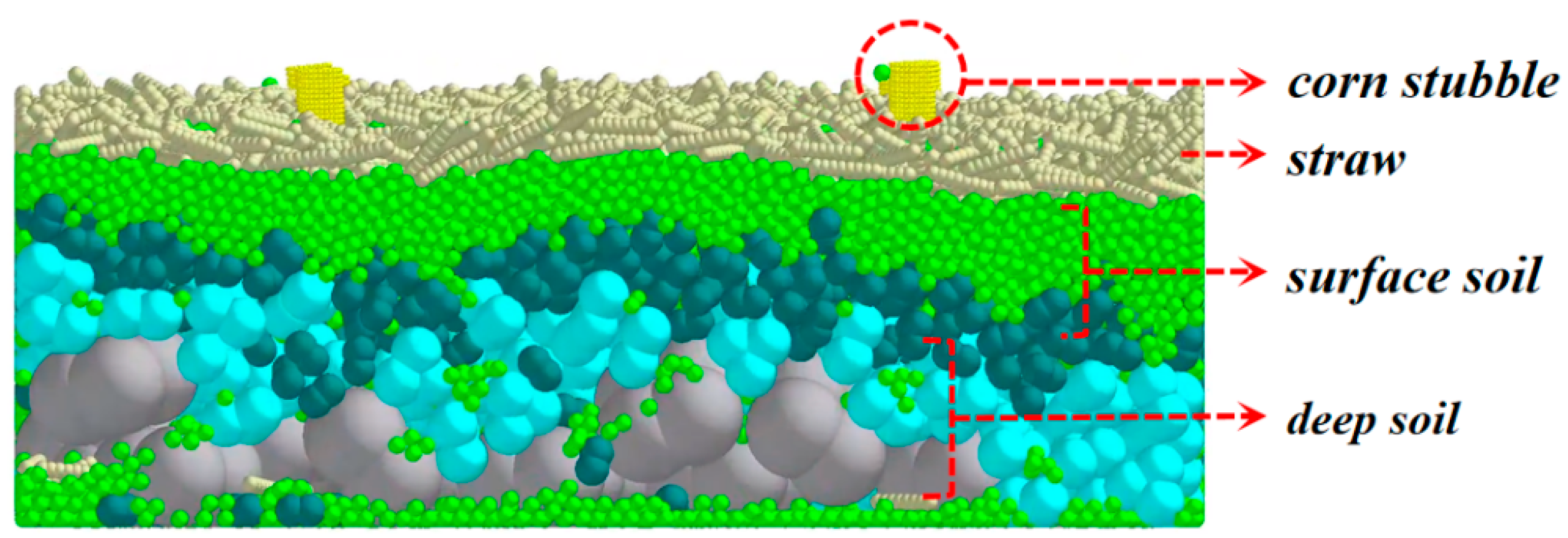
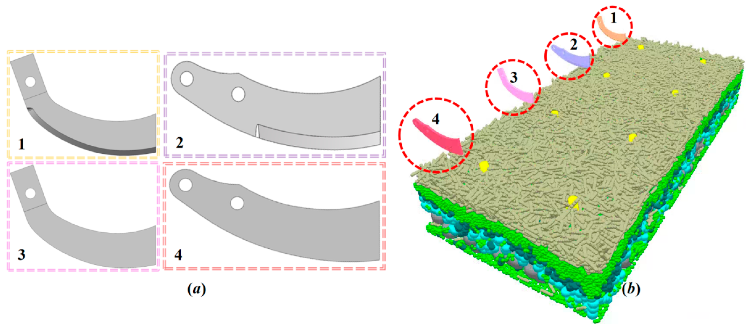
2.1.1. Design of Cutting Angles

The primary functions of the rotary blade include cutting, crushing, and turning soil, as well as incorporating cut stems and straw into the soil. The blade edge’s curvature is critical in this process. Agricultural requirements dictate that residual stems in the field should be evenly cut and mixed into the soil. However, when the edge becomes blunt or operates in heavy, sticky soil, the soil’s reaction force may be insufficient to support stem cutting. In such instances, the stems should glide along the edge rather than wrapping around it. Therefore, selecting an appropriate side cutting-edge curve is crucial. To design the side cutting-edge curve more effectively, it is essential to understand its functions and design requirements: 1. The blade edge should be optimized for sliding performance, ensuring that stems are either cut smoothly or expelled, thus preventing the blade shaft from becoming obstructed by entangled stems. 2. Cutting should commence near the blade handle to maximize cutting efficiency. 3. The edge curve’s shape should be as straightforward as possible, offered it meets the sliding performance requirements, to simplify manufacturing and implementation.

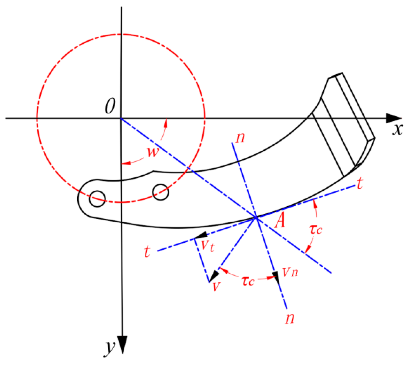
During operation, the rotary tiller’s blades revolve around the axis at an angular velocity w. Figure 1 illustrates that for any point A on the side cutting edge, the velocity at this point is v = rw, where r represents the distance from this point to the axis. A tangent t–t and a normal n–n intersect at point A. The speed v can be decomposed into two components: v_n, perpendicular to the cutting edge, and v_t, parallel to it. The ratio v_t/v_n = tgτ_c is referred to as the slip coefficient, with τ_c denoting the slip angle. The relationship between the slip angle and slip effect is crucial; an excessively small slip angle renders the slip effect negligible and ineffective, whereas an overly large slip angle increases the side cutting edge’s curvature, resulting in a larger overall tool size and associated issues such as increased power consumption. Considering these considerations, it is essential to conduct a computational analysis of the slip angle and its resulting effects.

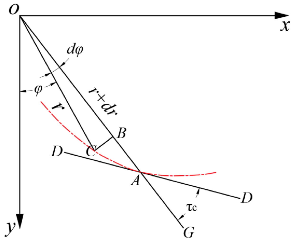
Figure 2 depicts the slip angle, typically defined as the angle between the radial line O–G at the cutting edge A and the tangent D–D. Let r = r(φ) be the polar coordinate equation for the cutting-edge curve. When φ increases by dφ, the change in the radial distance is dr. Therefore, AB = dr and BC = rdφ. The slip angle equation for the cutting edge can thus be expressed as follows:

$$\mathrm{tg}{\tau }_c={\displaystyle \frac{\mathrm{BC}}{\mathrm{AB}}}={\displaystyle \frac{rd\phi }{dr}}$$

(1)

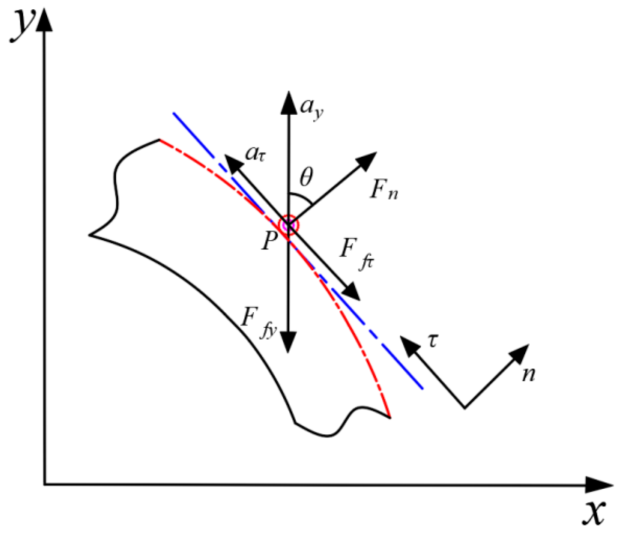
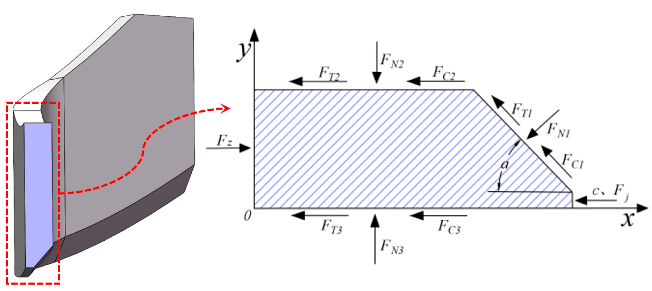
A dynamic model is developed to appraise the shear motion of the cutting edge in relation to the soil–root composite, with the aim of determining the critical conditions for slip. A two-dimensional coordinate system is established, where the y-axis represents the forward direction of the cutting edge, and the x-axis denotes its tangential direction. Figure 3 illustrates the relative position of a particle P to the cutting edge.

As the side cutting edge advances along the positive y-direction, the slip particle P experiences a combined motion. This movement comprises a pull along the y-axis coupled with a downward cutting motion along the edge. Throughout this process, particle P is subject to three forces: the normal force exerted by the cutting edge, the frictional force from the soil–root composite, and the frictional force from the cutting edge itself. The dynamic equilibrium equation for the slip particle P can be expressed as follows:

$$\left\{\begin{array}{c}{F}_n-F_{fy}\cos \theta =m{a}_y\cos \theta \\ F_{fy}\sin \theta -F_{f\tau }=m\left(a_{\tau }-a_y\sin \theta \right)\end{array}\right.$$

(2)

In the equation, F_n—normal force at the cutting edge of the side cutting edge, N;

F_fy—frictional force exerted by the root–soil composite on sliding point P along the y-axis, N;

θ—sliding cut angle, (°);

m—mass of sliding point P, kg;

a_y—tangential acceleration along the y-axis, m/s²;

F_fτ—frictional force on sliding point along the tangent direction of the blade edge, N;

a_τ—acceleration of the sliding point along the tangent direction of the blade edge, m/s².

The side cutting edge’s action causes slip particle P to tend towards the positive y-direction, while the soil–root composite counters with a frictional force in the negative y-direction. Should relative sliding occur between the cutting edge and slip particle, a trend of relative motion will be observed. Accordingly, the frictional force F_fτ at point P along the edge can be expressed as follows:

$$F_{f\tau }=F_{n}f=F_n\tan \phi$$

(3)

In the equation, f—composite friction coefficient between the sliding point and the cutting edge of the side blade;

φ—friction angle between the sliding point and the cutting edge of the side blade, (°).

Substituting Equation (3) into Equation (2) and simplifying gives the following:

$$F_n\left(\tan \theta -\tan \phi \right)=m{a}_{\tau }$$

(4)

In typical operating conditions, the normal force F_n on the side cutting edge remains positive. When relative sliding takes place between the cutting edge and slip particle, the slip particle’s tangential acceleration must be positive (a_τ > 0). Equation (3) implies that θ > φ, suggesting the slip angle exceeds the friction angle between the cutting edge and slip particle. This friction angle may represent the friction between the cutting edge and soil, the cutting edge and roots, or a combination of both. Generally, the friction coefficient does not surpass 0.8, which corresponds to a friction angle of approximately 40°. Therefore, the side cutting edge’s slip angle must be greater than this friction angle. Additionally, to avoid excessively large tool dimensions resulting from an overly high slip angle, it is constrained in the range of 40° to 65°.

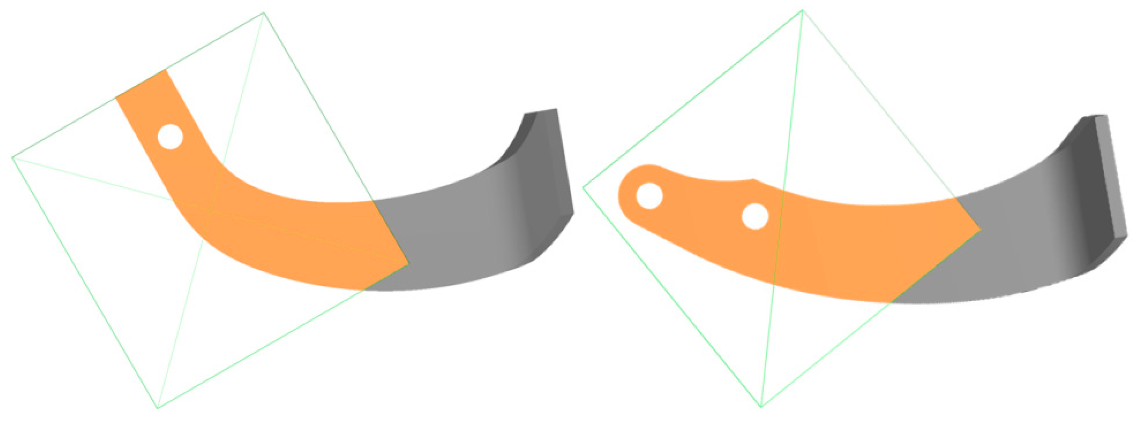
2.1.2. Design of Eccentric Circular Side Cutting Edges

The diversity in soil conditions, planting methods, and surface residue necessitates a range of cutting tools, as a single blade type cannot meet all tillage requirements. This has led to the creation of various blade designs incorporating different curves, such as equiangular spirals, Archimedean spirals, and sine–index curves. However, simplifying blade curves is crucial for enhancing tool design versatility and manufacturing efficiency, facilitating broader application. While these blade curves fulfill basic usage requirements, they present several challenges. Firstly, the design process often involves representing blade curves as a series of arc points connected by curves utilizing coordinate methods. This approach fails to fully reflect the regularity of the curves, rendering it challenging to accurately identify the blade’s characteristic curve type from design drawings. Therefore, this impedes an accurate evaluation and analysis of slip performance. In addition, defining the blade edge utilizing coordinate methods results in a lack of clear regularity in manufacturing and processing, thereby increasing the complexity and challenge of blade production and inspection.

Arcs, being the simplest curves after straight lines, offer advantages in both representation and manufacturing processes. Theoretical analysis indicates that an eccentric circular edge can achieve the slip performance of various blade curves [18]. Moreover, the slip angles at different positions on an arc can be determined through relatively simple methods, significantly facilitating blade manufacturing and performance analysis. After analyzing the side cutting-edge design curves of other tool types, including rotary blades, stubble breakers, and reclamation blades, it was determined that the rotary tiller side cutting-edge design would utilize an eccentric circular curve. The following section will offer a detailed explanation of the characteristics and design principles of the eccentric circular cutting-edge curve.

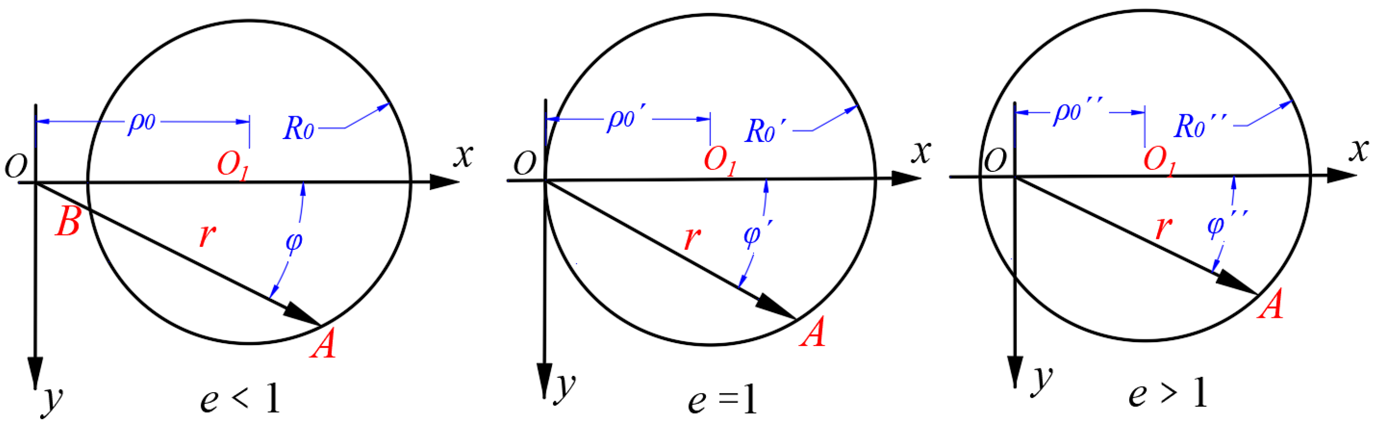
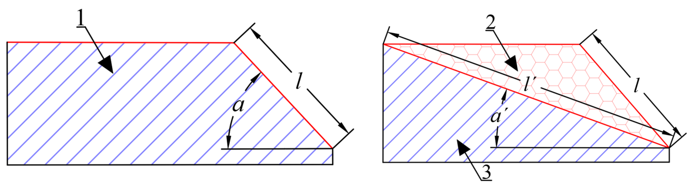
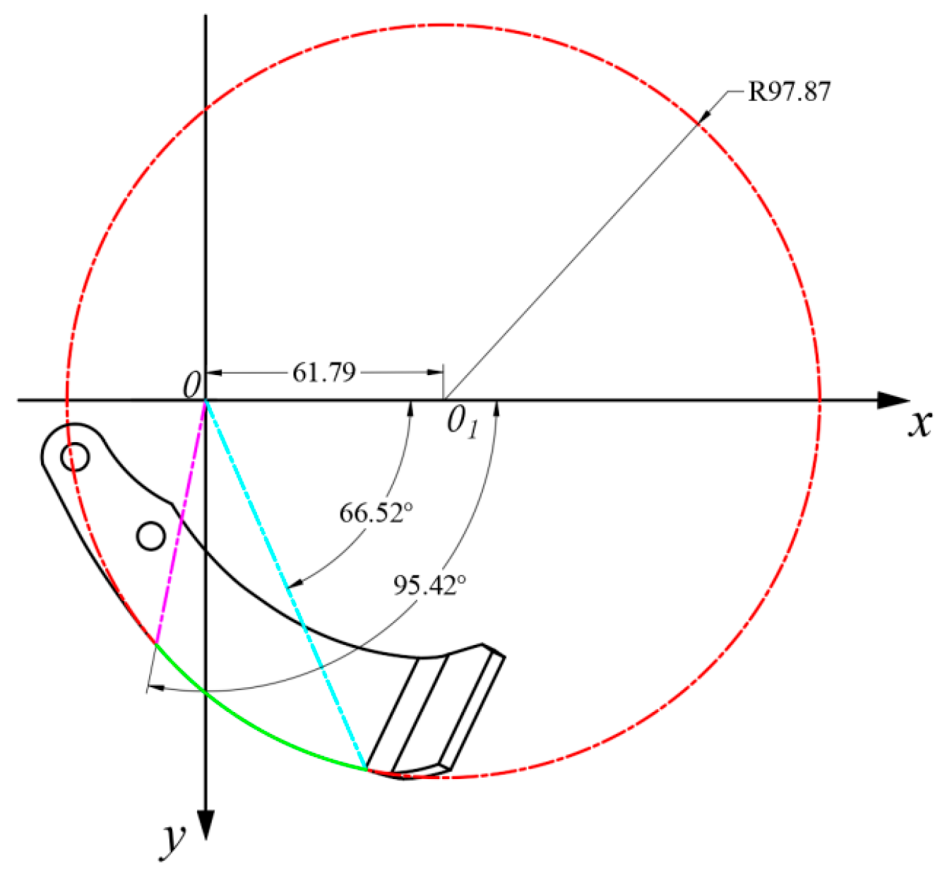
As presented in Figure 4, the eccentric circle with a radius of R₀ has its center O₁ on the x-axis, and its polar coordinate equation is given by Equation (5):

$$r^2-2r{\rho }_0\cos \phi +{{\rho }_0}^2={R_0}^2$$

(5)

$$r={\rho }_0\cos \phi {\rho }_0\sqrt{{({\displaystyle \frac{R_0}{{\rho }_0}})}^2-{\sin }^2\phi }$$

(6)

In the equation, ρ₀—distance from O₁ on the x-axis to the rotation center O;

R₀—radius of the eccentric circle;

φ—angle between the polar radius of any point A on the circle and the x-axis.

Taking the derivative of Equation (6) gives the following:

$${\displaystyle \frac{dr}{d\phi }}=-{\rho }_0\sin \phi +{\rho }_0{\displaystyle \frac{-\sin \phi \cos \phi }{\sqrt{e^2-{\sin }^2\phi }}}$$

(7)

Substituting Equations (5) and (6) into Equation (1) gives the following:

$$\mathrm{tg}{\tau }_c={\displaystyle \frac{\cos \phi +\sqrt{e^2-{\sin }^2\phi }}{-\sin \phi -\frac{\sin \phi \cos \phi }{\sqrt{e^2-{\sin }^2\phi }}}}=-{\displaystyle \frac{\sqrt{e^2-{\sin }^2\phi }}{\sin \phi }}$$

(8)

The negative sign in the above equation indicates that φ increases as r decreases; therefore, it is omitted to obtain Equation (9).

$${\tau }_c=t{g}^{-1}\left({\displaystyle \frac{\sqrt{e^2-{\sin }^2\phi }}{\sin \phi }}\right)$$

(9)

From Equation (9), it is clear that the slip angle τ_c is a function of only the eccentric distance e and the polar angle φ. To illustrate the relationship between the slip angle τ_c and the eccentric distance e and polar angle φ, specific values of e were selected. The corresponding relationships between the slip angle and polar angle were computed utilizing Equation (9) and plotted as a curve graph (Figure 5). We observed that for a constant value of φ, an increase in the eccentric distance leads to a corresponding increase in the slip angle. By varying the eccentric distances and ranges of polar angles, we can obtain blade curves with different slip characteristics. Before designing the side cutting-edge curve, it is necessary to determine the roller radius R based on tillage requirements and rotary tiller conditions, which corresponds to the radius of the eccentric circle. Following this, we must measure the minimum working radius r₀ and the radius r₁ at the bending line. As the dimensions of the RA rotary blade are an improvement on the IT260 rotary blade, we will continue to use the values of r₀ and r₁ from the IT260 blade. To simplify the design process, the polar angle φ₀ corresponding to the initial working radius r₀ remains unchanged. In summary, the design parameters for the RA rotary blade side cutting edge are the eccentric distance e, the polar angle φ₁ at r₁, and the slip angle τ_c at r₁.

Drawing from design experiences with other blade types [18], the polar angle φ₁ is limited to a range of 40° to 100°, while the cutting angle τ_c is confined between 40° and 65°, as specified by Formula (4). Figure 5 illustrates these constraints, with pink and green lines representing the ranges of the polar angle φ₁ and the cutting angle τ_c, respectively. The red curve in this domain depicts cutting characteristics across various eccentricities. This parameter space defines the experimental factor levels. The evaluation criterion is based on cutting resistance under different parameters, and an orthogonal experimental approach is utilized to identify the optimal parameter combination.

2.2. Design of the Cutting Edge Angle for RA Rotary Blade

2.2.1. Analysis of Cutting-Edge Stress

Rotary tillage involves the sequential engagement of the side cutting edge and tangential edge of the rotary blade with the soil. This process comprises periodic compression, cutting, fragmentation, and throwing to accomplish tillage. Figure 6 presents a cross-sectional view of the rotary blade for force analysis. The forces that must be overcome include soil adhesion, resistance from soil compaction, friction and adhesion between soil and blade, and shear resistance from corn residue and straw. Considering the positive direction as rightward along the x-axis and upward along the y-axis, the forces acting on the rotary blade in the x and y directions are as follows:

$$\sum _i^n{X}_i=0, F_z-F_{T2}-F_{T3}-F_{C2}-F_{C3}-\left(F_{T1}+F_{C1}\right)\cos \alpha -F_{N1}\sin \alpha -F_j-c=0$$

(10)

$$\sum _i^n{Y}_i=0,\hspace{1em}\hspace{1em}{F}_{N3}-F_{N2}-F_{N1}\cos \alpha =0$$

(11)

In the equation, n represents the number of forces; X_i denotes the i-th force (in N) projected in the x-direction for the national standard rotary blade; Y_i expresses the i-th force (in N) projected in the y-direction for the IT260 rotary blade.

When considering friction, F_T1, F_T2, and F_T3 represent the sliding friction forces of the soil relative to the surface of the rotary blade. The formula for the sliding friction force is as follows:

$$F_{Ti}=\mu F_{Ni}\hspace{1em}(i=1, 2, 3)\hspace{1em}\hspace{1em}{F}_N=P_i{A}_i$$

(12)

In the equation, F_Ti represents the i-th friction force applied to the blade, N; μ denotes the coefficient of sliding friction; μ = tanφ; F_Ni expresses the i-th normal force applied to the blade, in N. Substituting Equation (12) into Equation (11) yields the following, where F_T3 is

$$F_{T3}=F_{T2}+F_{T1}\cos \alpha$$

(13)

Substituting Equation (13) into Equation (10) yields the following, where the result for F_Z is

$$\begin{array}{ll}{F}_Z& =2F_{T2}+2F_{T1}\cos \alpha +F_{N1}\sin \alpha +F_{C2}+F_{C3}+F_{C1}\cos \alpha +F_j+c\\ & = 2F_{T2}+F_{N1}(2\mu \cos \alpha +\sin \alpha )+F_{C2}+F_{C3}+F_{C1}\cos \alpha +F_j+c\end{array}$$

(14)

Equation (14) demonstrates that cutting resistance F_Z is influenced by normal pressure F_Ni, the coefficient of sliding friction μ, and the cutting-edge angle α. As F_Ni increases, so does the cutting resistance, indicating greater soil hardness. Similarly, a higher coefficient of sliding friction μ leads to increased cutting resistance, assuming other factors remain constant. The cutting resistance also rises with an increase in the cutting-edge angle α [19]. Research suggests that the optimal cutting-edge angle for rotary blades in soil cutting is between 20° and 45° [20]. For practical manufacturing purposes, national standard rotary blades typically feature a 45° bevel on the cutting edge [21]. Therefore, reducing the cutting-edge angle while increasing blade width results in a sharper blade, thereby further decreasing cutting resistance. Figure 3 illustrates this concept: 1 represents the cross section of the national standard rotary blade, 2 indicates the removed portion, and 3 depicts the cross section of the modified blade.

2.2.2. Design of Cutting-Edge Angle Parameters

To determine the new cutting edge, a force analysis is conducted, as presented in Figure 5. The forces acting in the x and y directions are as follows:

$$\sum _i^n{X}_i=0, {F_z}^{\prime }-{F_{T2}}^{\prime }-{F_{C2}}^{\prime }-\left({F_{T1}}^{\prime }+{F_{C1}}^{\prime }\right)\cos {\alpha }^{\prime }-{F_{N1}}^{\prime }\sin {\alpha }^{\prime }-{F_j}^{\prime }-c^{\prime }=0$$

(15)

$$\sum _i^n{Y}_i=0,\hspace{1em}\hspace{1em}{F_{N2}}^{\prime }-{F_{N1}}^{\prime }\cos {\alpha }^{\prime }=0$$

(16)

Substituting Equation (12) into Equation (16) yields the following, where the result for F_T2’ is

$${F_{T2}}^{\prime }={F_{T1}}^{\prime }\cos {\alpha }^{\prime }$$

(17)

Next, substituting Equation (17) into Equation (15) yields the following, where the result for F_Z′ is

$$\begin{array}{ll}{F_Z}^{\prime }& =2{F_{T1}}^{\prime }\cos {\alpha }^{\prime }+{F_{N1}}^{\prime }\sin {\alpha }^{\prime }+{F_{C2}}^{\prime }+{F_{C1}}^{\prime }\cos {\alpha }^{\prime }+{F_j}^{\prime }+c^{\prime }\\ & = {F_{N1}}^{\prime }(2\mu \cos {\alpha }^{\prime }+\sin {\alpha }^{\prime })+{F_{C2}}^{\prime }+{F_{C1}}^{\prime }\cos {\alpha }^{\prime }+{F_j}^{\prime }+c^{\prime }\end{array}$$

(18)

After comparing Equations (14) and (18), we observe that when a ≤ 45°, 2μcosa + sina approximates 2μcosa′ + sina′. Neglecting the soil adhesion force F_Ci allows for a simplification of Equations (14) and (18) to

$$F_Z= 2F_{T2}+2F_{T1}+F_j+c$$

(19)

$${F_Z}^{\prime }= 2{F_{T1}}^{\prime }+{F_j}^{\prime }+c^{\prime }$$

(20)

Assuming a consistent cutting-edge thickness, C and F_j are considered equivalent. An analysis of F_Z and F_Z′ in Equation (12) indicates that, considering a constant coefficient of kinetic friction μ, F_Ti exhibits a positive correlation with F_Ni. For a given unit load on the tool (i.e., uniform loading), the normal pressure is proportional to the bearing area. As depicted in Figure 7, the red-shaded area forms an obtuse triangle, with the original cutting-edge section represented by the two shorter sides and the new design’s cutting-edge section by the hypotenuse. The combined length of the two shorter sides surpasses that of the hypotenuse, resulting in a smaller cutting-edge section area for the new angle. Therefore, this leads to a reduced normal pressure, i.e., F_Z′ < F_Z.

To identify the cutting-edge angle a that minimizes soil penetration resistance, we can derive the second derivative of Equation (18):

$$f^{″}(a)=P_i\cdot A_i\cdot (-2\mu \sin a-\cos a)-F_{Ci}\cos a$$

(21)

The cutting-edge angle a can be derived as follows:

$$a={\tan }^{-1}\left(-{\displaystyle \frac{2\mu P_i{A}_i+F_{Ci}}{P_i{A}_i}}\right)$$

(22)

In loamy soil conditions, the coefficient of sliding friction μ and soil adhesion force are reported as 0.4 ± 0.1 and (2.6 ± 1.2) N, respectively [22]. Calculations based on these values yield a cutting-edge angle a of 26.57°. Considering the precision requirements in actual production and processing, a buffer range has been set, expanding the parameter range to 26°–27° (Figure 8).

2.3. Design of the RA Rotary Blade Handle

The primary objective in designing the RA rotary blade is to reduce blade breakage. The most common failure point is at the neck where the blade attaches to the handle. Therefore, analyzing the handle design is more crucial than modifying the blade shape. Essentially, reimagining the handle to address blade breakage represents an innovative approach.

The operational environment for clearing blades is known to be relatively harsh; however, breakage is less severe compared to rotary blades. Accordingly, improvements were made to the clearing blade handle while maintaining the dual-bolt hole design. By incorporating the operational requirements of the rotary tiller, the handle was optimized to reduce weight and enhance structural integrity, offering improved breakage resistance while meeting working conditions. Figure 9 illustrates the enhanced handle design. With a rotational radius of 260 mm, the distance from the center of the two bolt holes to the rotation center is set at 75 mm, and the bolt hole spacing is established at 51 mm in accordance with national standards for clearing blades. The bolt holes have a diameter of 14 mm, utilizing M14 countersunk bolts to ensure compatibility with commonly available clearing blades and enhance tool versatility. Static analysis indicates that stress concentrates around the bolt holes during operation. To ensure uniform stress distribution between the bolt holes and the sidewall, the handle shape was adjusted to maintain a safety distance from the handle boundary to the center of the bolt holes, allowing for better stress relief. As indicated by the green dimensions, the shortest distance from the bolt hole center to the handle boundary is 20 mm. The exact positions of the two holes were determined by specifying the relevant dimensions.

The handle profile consists of four curved segments, as depicted in Figure 9. The initial curve aligns tangentially with the blade’s back curve, facilitating a smooth transition while maintaining a minimum 20 mm distance from any point on the curve to the front bolt hole’s center. The second curve, an 80 mm diameter arc, corresponds to the blade axis size, ensuring a secure fit between the handle and axis. This arrangement offers support and distributes pressure from the front bolt hole. The third curve, a 20 mm radius arc concentric with the rear bolt hole, ensures that the handle edge remains at least 20 mm from the bolt hole’s center. The final curve, resembling the first, is tangent to the side cutting edge, ensuring a smooth structural transition.

2.4. Establishment of the Discrete Element Model for Soil–Root Composite

2.4.1. Development of a Flexible Model for Corn Residues

To ensure accurate modeling, researchers conducted sampling at the corn rotation test field in Yixian, Baoding City, Hebei Province (Figure 10a). The corn residues, comprising stalks, branching roots, and fine roots, were isolated by carefully removing soil clumps and particles surrounding the root system. The cross-sectional view of the corn residue root system is illustrated in Figure 10b. Analysis indicated that each corn plant contains an average of 24 single roots (SRs) with a mean length of 118.15 mm. The SR diameter distribution spans from 0 to 3 mm, decreasing as depth increases. To improve the authenticity and computational efficiency of subsequent DEM modeling, each SR was segmented into three portions with radii of 1.4 mm, 1.2 mm, 1 mm, and 0.8 mm (Figure 10c).

To enhance the accuracy of the discrete element model for soil–composite interactions and simulate the crushing effect of the rotary tiller on corn residue, we developed a flexible body model utilizing meta-particles. This model was developed based on the size parameters and morphological characteristics of corn residue. It comprises 1462 stalk particles and 1196 root particles, with the bonding links between particles illustrated in Figure 11a. We employed particles of varying radii to represent the dense, organized structure of corn stalks and the varying thickness of roots. Different colors were utilized to indicate particle sizes (Figure 11b).

Table 1. Parameters of the corn residue contact model.

Contact Model	Normal Stiffness of Bond (N/m−3)	Tangential Stiffness of Bond (N/m−3)	Critical Stresses of Bond (Pa)
1.4 mm–1.4 mm	6.5 × 109	7 × 109	5 × 108
1.4 mm–1.3 mm	6.5 × 109	7 × 109	5 × 108
1.4 mm–1.2 mm	6.5 × 109	7 × 109	5 × 108
1.4 mm–1 mm	6.5 × 109	7 × 109	5 × 108
1.3 mm–1.3 mm	5.4 × 109	6 × 109	5 × 108
1.3 mm–1.2 mm	5.4 × 109	6× 109	5 × 108
1.2 mm–1.2 mm	5.4 × 109	5 × 109	5 × 108
1.2 mm–1.1 mm	5.4 × 109	5 × 109	5 × 108
1.2 mm–0.8 mm	5.4 × 109	5 × 109	5 × 108
1.1 mm–1.1 mm	3.7 × 109	4 × 109	5 × 108
1.1 mm–1 mm	3.7 × 109	4 × 109	5 × 108
1 mm–1 mm	2.5 × 109	3 × 109	5 × 108
1 mm–0.8 mm	2.5 × 109	3 × 109	5 × 108
0.8 mm–0.8 mm	2 × 109	3 × 109	5 × 108

lists the model parameters.

In developing the stalk portion of the corn residue flexible model, we arranged spherical particles of different diameters in concentric rings, stacking them layer by layer along the z-axis. This approach accurately replicates the dense internal structure of the stalk. However, the modeling process presented a challenge: while the external diameter of the stalk was known, the diameters and quantities of particles required for each internal ring remained uncertain. The primary difficulty in modeling lay in determining the spatial coordinates of each particle in the annular structure to ensure a regular and dense bonding pattern.

To address this issue, a static compilation software was developed to calculate the spatial positions of the particles, with its visualization interface demonstrated in Figure 12. First, the number of rings in the tangential plane is established to determine the radius and quantity of particles in each ring. Based on the corn stalk’s physical model, the structure becomes more compact towards the center, resulting in a decrease in particle radius centrally. Then, the radius and number of particles in each ring are calculated to ensure sufficient spacing between particles, avoiding overlap. Following this, the number of layers stacked along the z-axis is determined to increase the structure’s density while maintaining overall dimensions. Finally, the spatial coordinate data of the particles are generated.

2.4.2. Selection of the Discrete Element Contact Model

Considering the complex characteristics of corn residue and the various changes in its fragmented form, the Hertz–Mindlin with Bonding model is utilized to constrain the residue’s shape and accurately simulate the cohesion between particles, as well as the fragmented state of the corn residue during tillage. The formation of Bonding connections between particles is depicted in Figure 13. The contact forces between stalks, soil particles, and residues are described in reference [23].

$$F_t^S=-S_t{\delta }_t$$

(23)

$$F_t^d=-2\sqrt{5/6}/\beta \sqrt{S_t{m}^{\ast }}$$

(24)

$$F_n^s=4E^{\ast }\sqrt{R^{\ast }}{\delta }_n^{3/2}$$

(25)

$$F_n^d=-2\sqrt{5/6}\beta \sqrt{S_n{m}^{\ast }}{\delta }_n$$

(26)

In this equation, F_{t s} and F_{t d} represent the tangential elastic and damping forces (N), while F_ns and F_nd signify the normal elastic and damping forces (N). S_t and S_n indicate the tangential and normal stiffness, $S_t=8G^{\ast }\sqrt{R^{\ast }{\delta }_n},S_n=2E^{\ast }\sqrt{R^{\ast }{\delta }_n}$, N/m; G^* expresses the equivalent shear modulus, $G^{\ast }=G_1{G}_2/(G_1+G_2)$, Pa; G₁ and G₂ depict the shear moduli of the contact materials (Pa); and R^* refers to the equivalent contact radius. $R^{\ast }=R_1{R}_2/(R_1+R_2)$, m; R₁ and R₂ stand for the contact radii of the two objects (m); and m^* depicts the equivalent mass. $m{,}^{\ast }=m_1{m}_2/(m_1+m_2)$, kg; m₁ and m₂ illustrate the masses of the contacting objects (kg); and E^* explains the equivalent Young’s modulus. $E^{\ast }=E_1{E}_2/[E_1(1-{\upsilon }_2^2)+E_2(1-{\upsilon }_1^2)]$, Pa; E₁ and E₂ symbolize the elastic moduli of the two contacting objects (Pa); υ₁ and υ₂ reflect their Poisson’s ratios; and β demonstrates constants. $\beta =-\ln \xi /\sqrt{{\ln }^2\xi +{\pi }^2}$, $\xi$ suggests the coefficient of restitution.

2.4.3. Development of the Straw Model

Extensive research has been conducted on the mechanical properties of rice and wheat straw, both domestically and internationally, leading to the establishment of well-founded models. In this study, the primary function of the rotary tiller is to bury the straw and stubble scattered on the surface during operation, rather than cutting or grinding them. Accordingly, the straw model developed for this study was simplified. A selection of straw samples was made, and their lengths and diameters were measured. A box plot (Figure 14a) demonstrates that the median length of the straw is 56 mm, while the median diameter is 5.3 mm. The model is developed utilizing a rigid structure, comprising straw particles with a density of 0.227 g/cm³, a Poisson’s ratio of 0.4, and a shear modulus of 1.0 × 10⁶ Pa [24]. It consists of 8 particles, each with a radius of 5 mm, and the center-to-center distance between adjacent particles is 5.4 mm. The total length of the straw model is 54 mm, as illustrated in Figure 14b.

2.4.4. Development of the Soil Bin Model

Soil samples were obtained through a five-point sampling method at Kongshan Slope, Yixian County, Baoding City, Hebei Province (E 114°51′–115°37′, N 39°02′–39°35′). Measurements were taken of the soil’s moisture content, density, and hardness at various depths. The area is represented by sandy loam soil with a clearly stratified structure, indicating significant differences in particle size and structure from the surface downward. Accordingly, four particle models were developed with diameters of 5 mm, 10 mm, 15 mm, and 20 mm (Figure 15), corresponding to 6.89%, 10.47%, 68.25%, and 14.39% of the total composition, respectively [25]. A soil box model with dimensions of 1500 mm × 1000 mm × 300 mm (Figure 16) was developed, featuring particles distributed from the surface to the bottom layer. The Hertz–Mindlin with Bonding model was chosen for soil particle contact, as it effectively replicates the soil properties under natural conditions and reflects soil fragmentation during tillage by monitoring bonding breakage rates. The simulation parameters are as follows: the soil particle model has a density of 1709 kg/m³, a Poisson’s ratio of 0.38, and a shear modulus of 1.0 × 10⁶ Pa; the 65Mn model has a density of 7830 kg/m³, a Poisson’s ratio of 0.3, and a shear modulus of 7.9 × 10¹⁰ Pa. The coefficients of restitution and friction are specified as follows: soil–soil restitution coefficient 0.6, static friction coefficient 0.6, dynamic friction coefficient 0.4; soil–straw restitution coefficient 0.5, static friction coefficient 0.5, dynamic friction coefficient 0.05; soil–65Mn steel restitution coefficient 0.6, static friction coefficient 0.6, dynamic friction coefficient 0.05; straw-straw restitution coefficient 0.3, static friction coefficient 0.3, dynamic friction coefficient 0.01; straw–65Mn steel restitution coefficient 0.3, static friction coefficient 0.3, dynamic friction coefficient 0.01 [26].

2.5. Comparative Validation Experiment

2.5.1. Comparative Validation Experiment of Cutting Resistance

To verify the eccentric circular side cutting-edge theory and the cutting-edge angle design, we conducted a comparative experiment between the RA and IT260 rotary blades. We focused solely on the side-cutting edge as the primary working edge to eliminate interference from the straight cutting edge and transition sections on cutting resistance. Considering that both the side cutting-edge curve and the cutting-edge angle directly affect cutting resistance, we selected this parameter as our evaluation criterion. We modeled the IT260 rotary blade under identical conditions for comparison. As illustrated in Figure 17a, both tools were initially unsharpened. By comparing the cutting resistances of these two sets, we aimed to confirm the viability of the eccentric circular side cutting-edge curve. In addition, we utilized unsharpened tools as the control group and sharpened tools as the experimental group to evaluate the benefits of the newly designed cutting-edge angle. Figure 17b depicts the cutting process (Figure 17).

2.5.2. Comparative Validation Experiment of Rotary Blade Resistance to Fracture

The RA rotary blade handle’s design aims to alleviate neck stress and minimize stress concentration, thus enhancing its resistance to breakage and longevity. To assess its durability, a comparative experiment was conducted with the IT260. The rotary blade’s 3D model was imported into ANSYS for static analysis. Fixed constraints were applied at the bolt holes and blade holder interface while a 500 N vertical external load was applied at the side cutting edge. Due to differences in mass and structural configuration between the two tools, the location and intensity of stress concentration vary. Relying solely on maximum equivalent stress as an evaluation criterion would only account for the blade’s stress and deformation, overlooking the effect of material volume and mass variations, potentially leading to less convincing results. To address this limitation, specific strength structural efficiency and specific stiffness structural efficiency were introduced as novel evaluation metrics. By incorporating material mass alongside maximum equivalent stress and deformation, these metrics offer a more comprehensive assessment of the reinforcement’s performance, as illustrated in Formulas (27) and (28) [27].

$$\eta ={\displaystyle \frac{U_S/S_S}{S_W}}$$

(27)

$$\beta ={\displaystyle \frac{U_S/S_D}{S_W}}$$

(28)

In the equation,

η—specific strength structural efficiency;

β—specific stiffness structural efficiency;

U_S—structural ultimate strength, in MPa;

S_S—maximum structural stress, in MPa;

S_D—maximum structural deformation, in mm;

S_w—structural mass, in g.

As a soil-contacting component, the forces acting on the rotary blade are closely associated with soil particles. While static analysis only reflects stress distribution in a stationary state, a more comprehensive evaluation of different handles’ effectiveness in reducing neck stress necessitated the use of the discrete element method. The EDEM2022’s Geometry Bin feature was employed to monitor geometry movements in a selected range in real time. A detection area of 200 mm × 200 mm × 200 mm was established, including the handle and neck structure, as illustrated in Figure 18. To ensure accurate force detection, three-dimensional coordinates were configured to synchronize with the rotary tiller assembly.

The longevity of the rotary blade, as a wear-prone component, significantly affects the reliability and cost-effectiveness of the equipment. While the analysis suggests that the RA rotary blade more effectively alleviates stress concentration and reduces neck stress compared to the IT260 over a few cycles, thus offering some resistance to breakage, the limited number of cycles precludes a comprehensive validation of its breakage resistance reliability. Therefore, conducting a fatigue life analysis of the RA rotary blade is crucial for identifying potential design flaws and assessing the validity of the design. Comparative experiments will determine whether the design meets expected performance standards, thereby evaluating the quality of the design results. While traditional lifespan prediction methods, such as fatigue testing, are widely used, they often incur significant time and economic costs. In contrast, finite element analysis presents a more cost-effective and efficient alternative [28].

Under normal working conditions, the maximum equivalent stress experienced by the rotary blade is significantly lower than the yield strength of its material, categorizing its potential failure mode as high-cycle fatigue. The complex and inhomogeneity of soil subjects the rotary blade to fluctuating stresses, resulting in irregular vibrations that may induce linear fatigue fractures at stress concentration points. First, the fatigue tool in ANSYS was employed to establish the S–N curve specific to the 65Mn material. Then, a CAE model of the rotary blade was developed, and fatigue life analyses were conducted on both RA and IT260 blades utilizing random cyclic loads generated by EDEM software. Currently, the predominant method for assessing linear fatigue accumulation damage involves the application of the Palmgren–Miner linear cumulative damage rule to estimate the component’s fatigue life [29].

$$D=\sum _{i=1}^k{D}_i=\sum _{i=1}^k{\displaystyle \frac{n_i}{N_i}}$$

(29)

In this equation, D_i signifies the damage inflicted by the i-th load stress, where i = 1, 2, …, k. The term n_i represents the number of cycles of damage caused by the i-th load stress. The total damage is denoted by D, with D = 1 indicating the component’s fatigue failure. In addition, N_i corresponds to the fatigue life associated with the i-th load stress.

As the rotary blade penetrates the soil, it experiences significant effect forces, resulting in momentary blade deformation and the generation of internal stresses in the blade material. Should these internal stresses surpass the yield strength of the material, the blade may suffer permanent deformation or fracture. Therefore, it is crucial to incorporate fracture stress as an evaluation metric to assess the handle’s protective capacity for the neck under near-fracture conditions. By utilizing the explicit dynamics module, the rotary blade’s resistance to fracture is measured and translated into fracture stress values, facilitating an evaluation of its performance under extreme stress conditions.

In the field of engineering and design, the Figure of Merit (FoM) is a comprehensive metric used to evaluate overall design performance. In structural design, particularly when it involves material and mechanical properties, the evaluation criteria often differ in focus and are weakly correlated. This creates a need for a unified metric that links these various performance factors together. Therefore, two key factors—ultimate fracture stress and structural efficiency based on specific strength—are selected from the above criteria. The FoM, based on these factors, is defined as follows:

$$\mathrm{FoM}={\displaystyle \frac{{\sigma }_n}{\rho }}\cdot \eta$$

(30)

In the equation,

σ_n—ultimate fracture stress, in MPa;

ρ—material density, in kg/m³;

η—specific strength structural efficiency.

2.5.3. Validation Experiment for the Performance Quality of the RA Rotary Blade

(1) Validation Experiment for Root Fragmentation Rate

The corn residue model initially comprises 15,056 bonds. In the visual representation, only the bonding connections between residue particles are visible, with soil and residue model particles concealed. As the rotary blade progresses through the material, the bonding connections in the residue model incrementally reach their stress thresholds, leading to the breakdown of these bonding areas. Figure 19 illustrates the fracture process of the bonding zones in the residue model.

(2) Validation Experiment for Soil Fragmentation Rate

In accordance with GB/T 5668-2008 on Rotary Blades [30], the selected parameters consist of a blade shaft speed of 300 r/min, a forward speed of 4.10 km/h, and a tilling depth of 180 mm. The simulation spanned 1.5 s, with analysis focusing on 1 s of stable operation. To ensure reliability, the experiment was conducted thrice, deriving an average value. At the outset, the side cutting edge of the rotary blade makes contact with and runs parallel to the soil surface, resulting in near-instantaneous blade entry. Considering the research objectives and existing knowledge, the soil fragmentation rate and straw coverage rate were identified as the primary parameters of interest. Figure 20 depicts the simulation process. To manage the significant number of particles efficiently, a dynamic calculation domain, defined by the red grid area, was implemented. Throughout the simulation, adjustments to the size and position of this domain optimized computational resources, thereby enhancing simulation efficiency and accuracy. Calculations were limited to particles in the dynamic domain, while those in other areas (white regions) remained stationary. This approach significantly improved computational efficiency and reduced processing time.

The soil fragmentation rate is conceptualized as the proportion of severed bonding connections in a unit volume relative to the initial number of connections. Samples were obtained 500 mm from the rotational axis following tiller operation. EDEM’s grid function facilitated the establishment of a grid solver with dimensions of 1000 × 500 × 250 mm for computational purposes. Figure 21 illustrates the positioning of the sampling site. The fragmentation rate was derived from calculations at ten different sampling locations, with the mean value being utilized.

(3) Validation Experiment for Straw Coverage Rate

The straw coverage rate is computed by comparing the quantity of straw model remnants on the surface post-tilling to the pre-tilling amount. EDEM’s grid function was employed to designate an area of 1000 mm × 1000 mm × 250 mm and conduct vertical layer analysis. First, the mass of straw in the surface layer was measured prior to tilling. Then, the mass of all straw in the designated surface area was measured post-tilling, with repeated measurements conducted utilizing varying detection areas (Figure 22).

2.6. Field Experiment

2.6.1. Testing Conditions

To evaluate the RA rotary blade’s performance in real-world conditions, field experiments were carried out in Yixian, Baoding City, Hebei Province (E 114°51′–115°37′, N 39°02′–39°35′). A typical hilly area was chosen, as depicted in Figure 23a, offering uniform environmental testing conditions. The experimental plot measured 50 m in length and 32 m in width, with 10 m buffer zones on each side. The trials incorporated four test routes, each separated by an 8 m interval. As presented in Figure 23b, the testing equipment consisted of a 60-horsepower tractor and a rotary blade. Prior to the trials, all instruments and equipment were thoroughly inspected and calibrated to ensure that measuring devices were in their specified valid calibration periods.

Table 2. Experimental equipment.

Name	Model/Specification
Steel ruler	0~30 cm
Steel tape	J19-50/0~5 m
Stop watch	HS-30 W/0~100 h
Stratometer	TYD-2/0~100 kg
Electric blast drying oven	DHG-9076A/50~300 °C
Electronic balance	NS-3200B/0–3200 g
Soil sampling box	1 × 1 m
Temperature/humidity meter	DT-321S, −30 °C~100 °C, 0%~100%RH

offers a comprehensive list of the primary testing instruments utilized.

2.6.2. Index and Factor of Test

The soil fragmentation rate was evaluated in compliance with established tillage quality standards. A 1 m × 1 m soil sampling frame was employed to define the sampling area, from which soil clods were extracted throughout the entire tilled layer. These clods were classified into three size groups: 0–2 cm, 2–4 cm, and exceeding 4 cm. The fragmentation rate was computed as the percentage of the total soil mass in the 0–4 cm range relative to the overall mass, with one measurement taken for each pass. Figure 24 illustrates the methodology employed for determining the fragmentation rate.

The sampling location for measuring the straw coverage rate corresponds to the site utilized for evaluating the fragmentation rate. The procedure begins by carefully removing and weighing the straw in the surface layer, which is then returned to its original position. After tilling, the straw in the surface layer is weighed once more to calculate the coverage rate. One measurement is recorded for each pass, and the straw coverage rate is determined by expressing the mass of straw collected post-tilling as a percentage of the total mass prior to tilling. Figure 25 offers a visual representation of the methodology employed for measuring the straw coverage rate.

3. Results

3.1. Analysis of the Orthogonal Optimization Results for the Eccentric Circular Side Cutting Edge

Orthogonal experiments were designed utilizing Design-Expert 13 software in accordance with the factor level codes outlined in

Table 3. Simulation test level factors and coding.

Level	A: e	B: τc	C: φ1
−1	1.1	50	40
0	1.65	57.5	70
1	2.2	65	100

. The results of these experiments are comprehensively presented in

Table 4. Orthogonal experimental results.

NO.	A: e	B: τc	C: φ1	Cutting Resistance F (N)
1	1.65	50	40	416.58
2	2.2	65	70	412.67
3	2.2	57.5	40	418.77
4	1.65	57.5	70	412.75
5	1.1	57.5	40	441.32
6	1.1	50	70	421.48
7	1.1	65	70	480.24
8	1.65	65	100	426.91
9	2.2	57.5	100	415.87
10	2.2	50	70	436.37
11	1.65	57.5	70	415.07
12	1.65	57.5	70	418.77
13	1.65	57.5	70	416.53
14	1.65	50	100	423.96
15	1.1	57.5	100	444.97
16	1.65	57.5	70	417.69
17	1.65	65	40	441.85

.

Utilizing the data analysis capabilities of Design-Expert 13, the fitted regression equation for cutting resistance F was formulated, as depicted in Equation (31).

Table 5. Analysis of variance of cutting resistance regression model.

Source of Variation	Sum of Squares	df	Mean Square	F-Value	p-Value
Model	4788.29	9	532.03	101.43	<0.0001
A	1360.59	1	1360.59	259.38	<0.0001
B	500.54	1	500.54	95.42	<0.0001
C	5.80	1	5.80	1.11	0.3281
AB	1699.91	1	1699.91	324.07	<0.0001
AC	10.73	1	10.73	2.04	0.1958
BC	124.55	1	124.55	23.74	0.0018
A2	628.52	1	628.52	119.82	<0.0001
B2	364.97	1	364.97	69.58	<0.0001
C2	14.45	1	14.45	2.76	0.1409
Residual	36.72	7	5.25
Lack of fit	14.61	3	4.87	0.8814	0.5222
Pure error	22.11	4	5.53
Sum	4825.01	16
R2 = 0.9924 APrecision = 38.3199 C.V. = 0.5362%

offers a detailed presentation of the variance analysis results for the regression model.

F = 416.16 − 13.04A + 7.91B − 0.8512C − 20.62AB − 1.64AC − 5.58BC + 12.22A² + 9.31B² + 1.85C²

(31)

Table 5 demonstrates the regression model’s p-value, which declines below 0.0001, indicating a high level of significance. The lack of fit p-value and F-value both surpass 0.05, indicating the model’s high fitting accuracy. With an R² value of 0.9924, the model exhibits a robust correlation. The signal-to-noise ratio (A_Precision) of 38.3199, significantly exceeding 4, points to remarkable reliability and accuracy. Additionally, the coefficient of variation (C.V.) of 0.5362% reflects the model’s excellent stability. A study of the p-values indicates that parameters A, B, AB, A², and B² produce a significant effect on cutting resistance.

Figure 26a illustrates the relationship between eccentricity e, sliding angle τ_c, and cutting resistance. As eccentricity e increases, cutting resistance initially decreases before rising again, whereas an increase in sliding angle τ_c consistently leads to higher cutting resistance. The lowest cutting resistance occurs when both eccentricity e and sliding angle τ_c approach their median values, suggesting an optimal combination of these variables. The concentration of contour lines in the central area indicates rapid fluctuations in the response variable, while the sparse contour lines at the periphery imply smaller variations. Figure 26b presents a smooth response surface plot, illustrating the cumulative effect of sliding angle τ_c and polar angle φ₁ on cutting resistance. The gradual upward trend of the response surface demonstrates that concurrent increases in both independent variables result in higher cutting resistance, indicating a positive correlation with low sensitivity.

The prediction model is optimized for experimental parameters through the establishment of constraints and an objective function, as illustrated in Equation (32).

$$\left\{\begin{array}{l}\mathrm{Min} F(A,B,C)\\ 1.1\le A\le 2.2\\ 50\le B\le 65\\ 40\le C\le 100\end{array}\right.$$

(32)

The optimal parameters are determined as follows: an eccentricity e of 1.37 mm, a sliding angle τ_c of 56°, and a polar angle φ₁ of 95.42°. Figure 27 demonstrates a portion of the eccentric circle in red, which represents the curve of the RA rotary blade’s side cutting edge, depicted by a green line segment. The intersection where the pink line meets the eccentric circle marks the starting point of the side-cutting edge, while the intersection of the blue line with the eccentric circle indicates its endpoint. Utilizing the parameters highlighted in the figure, the equation of the eccentric circle is expressed in Equation (33).

$$r^2-131.84r\cos \phi +{65.92}^2={90.95}^2$$

(33)

3.2. Analysis of Cutting Resistance Results

Figure 28 presents the cutting resistance results, illustrating the maximum cutting resistance of IT260 and RA rotary blades in both sharpened and unsharpened conditions across three cutting cycles. As illustrated in Figure 28a, the unsharpened IT260 and RA rotary blades exhibit average maximum cutting resistances of 477 N and 449 N, respectively, indicating a 5.9% decrease. This observation verifies the eccentric circle side cutting-edge theory. Figure 28b indicates that the IT260 rotary blade’s average maximum cutting resistance drops from 477 N in the unsharpened state to 412 N when sharpened, marking a 13.6% reduction. Comparatively, Figure 28c demonstrates that the RA rotary blade’s average maximum cutting resistance decreases from 449 N to 381 N after sharpening, representing a 15.1% reduction. The more significant decrease in cutting resistance exhibited by the RA rotary blade implies that the newly designed cutting angle is more efficient in reducing resistance.

3.3. Analysis of the RA Rotary Blade Fracture Resistance Performance

3.3.1. Static Analysis

Figure 29 demonstrates that under identical external load conditions, the IT260 rotary blade experiences a maximum equivalent stress of 32.214 MPa, with stress concentration occurring at the blade’s neck, whereas the RA rotary blade exhibits a maximum equivalent stress of 27.382 MPa, with stress concentration near the front-end-threaded hole of the neck. A numerical comparison indicates that the RA rotary blade’s maximum equivalent stress is approximately 17.65% lower than that of the IT260 rotary blade. However, due to variations in mass and structural design between the two tools, the location and extent of stress concentration differ; therefore, comparing only the maximum stress does not offer a comprehensive account of the performance differences. Therefore, the specific strength and specific stiffness structural efficiencies of both tools were calculated and compared, utilizing data from static simulations. The results indicate that the RA rotary blade’s specific strength structural efficiency improved by 9.72%, while its specific stiffness structural efficiency increased by 9.78%. These findings demonstrate that the RA rotary blade outperforms the IT260 in minimizing deformation and stress concentration, aligning with the intended design objectives.

3.3.2. Analysis of Maximum Stress at the Blade Neck

Figure 30 illustrates the force variation observed in the IT260 and RA rotary blades during monitoring. To ensure result consistency, the force variation across three cutting cycles is presented. Both tools exhibit broadly similar working cycles, with peak forces occurring at similar points. Focusing on the stress concentration areas (the handle and neck), the IT260 rotary blade registers a maximum force of 114.67 N over the three cutting cycles, with an average maximum force of 109.33 N. In contrast, the RA rotary blade demonstrates a maximum force of 88.45 N and an average maximum force of 83.67 N. The neck of the IT260 rotary blade is subject to higher forces with more significant fluctuations, while the RA rotary blade experiences lower forces with more consistent peaks. Specifically, the RA rotary blade’s maximum force is 22.9% lower than that of the IT260, and its average maximum force is reduced by 23.5%. These findings indicate that the handle design of the RA rotary blade is effective, meeting design expectations and indicating consistent performance across multiple cycles.

3.3.3. Analysis of Fatigue Strength

Considering the actual surface roughness and potential microscopic damage of the blade, we set the fatigue strength factor (KF) to 0.8 [31]. We import the random cyclic load measured by EDEM software as historical data, adjusting the scale factor to 1.5. The material’s S–N curve and load spectrum are then corrected for mean stress utilizing the built-in program, followed by a fatigue life analysis. Figure 31 presents the resulting fatigue life contour map. This map indicates that under high-cycle fatigue loading, the neck of the IT260 rotary blade reaches its fatigue limit first, while the RA rotary blade demonstrates a fatigue limit in the area above the first screw hole at the connection to the blade back. When subjected to the same cyclic load, the fatigue life of the IT260 and RA rotary blades is measured in cycles, with values of 61,887 and 86,074 cycles, respectively, indicating a 39.08% increase. These findings suggest that the RA rotary blade design significantly extends its service life and lowers the risk of fracture.

3.3.4. Analysis of Ultimate Fracture Stress

To study the rotary blade’s handle and its influence on fracture mechanics, we employed ANSYS2019’s explicit dynamics module. This module was incorporated into the visual interface, where we assigned material properties to the geometry and performed meshing. We applied fixed constraints to the handle area and set the simulation duration to 0.1 s with a maximum of 10,000 iterations. Displacement constraints were imposed on the rotary blade’s cutting edge, side edge, and bending transition area, with vertical displacement applied until fracture occurred.

Figure 32 illustrates the ultimate fracture stress contour map. Fractures occur at the blade’s neck in both rotary blades. The color map indicates that at the moment of fracture, most of the IT260 blade’s handle is blue, suggesting it experienced relatively low stress. However, a green–yellow–red band near the handle’s end at the neck indicates stress concentration in this area, leading to fracture. In contrast, the RA rotary blade’s handle demonstrates a wider color spectrum at fracture, with overlapping blue, green, and yellow hues. This suggests that during crack formation, the handle effectively distributed stress, alleviating pressure from the neck and contributing to stress distribution and protection.

Comparing Figure 31 and Figure 32 indicates that crack development locations align with areas predicted to reach the fatigue limit first in the fatigue life forecast, verifying the fatigue life prediction. The ultimate fracture stress at failure for the IT260 and RA rotary blades is 956.73 MPa and 1216.7 MPa, respectively, representing a 27.17% increase. These findings indicate that the redesigned RA rotary blade’s handle can withstand greater stress at fracture, thus reducing stress concentration and offering more effective protection for the neck.

As shown in

Table 6. Comparison of static results.

Parameter	IT260 Rotary Blade	RA Rotary Blade	Contrast
Mass (g)	716.3	781.4	8.33%
Deformation (mm)	0.1402	0.1192	−17.61%
Maximum equivalent stress (MPa)	32.214	27.382	−17.65%
Specific strength structural efficiency	0.0325	0.0350	9.72%
Specific stiffness structural efficiency	7.4682	7.6055	9.78%
Maximum stress at the blade neck (N)	109.33	83.67	−23.47%
Fatigue strength (Times)	61,887	86,074	39.08%
Ultimate fracture stress (MPa)	956.73	1216.70	27.17%
FoMA	0.0194	0.0266	37.11%

, to visually present the comparison of the evaluation criteria between the national standard rotary blade and the RA rotary blade, all relevant data have been compiled into a single table for comparative analysis.

3.4. Analysis of Tillage Operation Indicators

3.4.1. Analysis of Residue Fragmentation Rate Results

The corn residue flexible body model comprises two primary components: the stalk and the root hairs. These elements exhibit different bonding mechanisms and parameter configurations, resulting in unique bonding characteristics. The stalk is developed from spherical particles of varying radii arranged in a circular pattern. Each spherical particle typically forms at least three bonds with adjacent particles, creating a dense network of bonds. Statistical analysis indicates that the stalk contains a total of 12,268 bonds. In contrast, the root hairs consist of spherical particles with varying radii arranged linearly, forming single bonds between adjacent particles, resulting in a significantly lower total of 2788 bonds. The fragmentation of corn residue occurs primarily through bond rupture. To reduce experimental variability, bond fracture data were collected from ten corn residue models, recording the number of bond fractures in both the stalk and root hair regions and calculating average values. As presented in Figure 33, the bond fracture process initially progresses rapidly before decelerating and eventually reaching a plateau. The stalk experiences approximately 7000 bond fractures, representing 60% of its total bonds, while the root hairs exhibit approximately 2500 bond fractures, accounting for 90% of their total bonds. These findings suggest that during rotary tillage, the root hairs demonstrate superior fragmentation, whereas the stalk tends to retain larger, strip-like residues post-tillage. This residual material can be incorporated into the soil as fertilizer, aligning with practical operational conditions and tillage quality requirements.

3.4.2. Analysis of Soil Fragmentation Rate and Straw Coverage Rate Results

When assessing the quality of rotary tiller operations, the soil fragmentation rate and straw coverage represent crucial indicators. To facilitate comparison,

Table 7. Results of soil fragmentation rate and straw coverage rate.

Measurement	Results of the Simulation Experiment		Results of the Field Experiment
	Soil Fragmentation RateY1 (%)	Straw Coverage RateY2 (%)	Soil Fragmentation RateY3 (%)	Straw Coverage RateY4 (%)
1	93.4	81.7	83.4	86.8
2	91.2	89.3	84.7	82.3
3	90.3	83.5	85.9	89.9
4	87.5	91.2	86.2	90.6
5	88.1	85.6	87.5	87.2
6	89.3	88.1	88.3	84.1
7	90.2	82.8	89.1	91.3
8	91.5	90.4	90.7	83.7
9	91.7	86.9	83.8	85.4
10	90.6	92.3	91	88.5
P	90.38	90.98	87.06	87.08
S	1.66	5.42	2.58	2.94
V(%)	1.84%	5.95%	2.96%	3.37%

presents data from both simulation experiments and field trials side by side. The simulation results demonstrated an average soil fragmentation rate (Y₁) of P = 90.38, accompanied by a standard deviation (S) of 1.66 and a coefficient of variation (V) of 1.84%. For the average straw coverage (Y₂), the values were P = 90.98, S = 5.42, and V = 5.95%, respectively. In the field trials, the average soil fragmentation rate (Y₃) was P = 87.06, with a standard deviation of S = 2.58 and a coefficient of variation of V = 2.96%. The average straw coverage (Y₄) was P = 87.08, with a standard deviation of S = 2.94 and a coefficient of variation of V = 3.37%. The error between Y₁ and Y₃ was 3.79%, while the error betweenY₂ and Y₄ was 4.48%. In accordance with GB/T 5668-2008 (National Technical Committee for Agricultural Machinery Standardization, 2008), the equipment’s soil fragmentation rate and straw coverage align with design specifications, indicating good stability and suitability for rotary tilling operations. With discrepancies between field and simulation experiments below 5%, the feasibility of discrete element simulations is confirmed.

4. Conclusions and Discussion

1. The side cutting-edge curve and cutting-edge angle were designed to reduce cutting resistance. An eccentric circular curve was developed for the RA rotary blade’s side cutting edge. Orthogonal experiments were conducted utilizing cutting resistance as the evaluation criterion to determine the optimal parameter combination, resulting in the most effective eccentric circular curve. Additionally, force analysis at the cutting edge indicated the optimal cutting-edge angle to be 26.57°.

2. Utilizing the discrete element method, a soil bin model and a flexible corn residue model were created. The cutting resistance of the IT260 and RA rotary blades was compared in both sharpened and unsharpened conditions. The findings exhibit that in the unsharpened state, the side cutting-edge resistance decreased by 5.9%. When the edge was sharpened and the new cutting-edge angle was applied, the resistance decreased by 15.1%, confirming the superiority of the eccentric circular side cutting edge and the newly applied cutting-edge angle.

3. The RA rotary blade’s handle was redesigned to improve fracture resistance and extend its service life. Metrics such as specific stiffness and specific strength efficiency were introduced, and the handle’s protective performance was evaluated utilizing criteria including maximum equivalent stress, maximum stress at the neck, fatigue life, and ultimate fracture stress. The results exhibit that, compared to the IT260 rotary blade, specific strength efficiency increased by 9.72%, specific stiffness efficiency improved by 9.78%, the average maximum stress at the handle decreased by 23.5%, fatigue life increased by 39.08%, and ultimate fracture stress rose by 27.17%. These findings confirm the handle’s effectiveness in enhancing fracture resistance.

4. Field trials were conducted to measure the soil fragmentation rate and straw coverage. The results were compared with simulation data, indicating an error margin of less than 5%, which confirms the feasibility of the simulation.

This study demonstrates the superior performance of the RA rotary tiller blade through its design, optimization, validation, and comparative analysis. The blade shows significantly improved resistance to breakage, extended lifespan, and reduced labor costs. However, real-world field operations may introduce uncontrollable factors that could challenge the applicability of the findings. Future research will involve field tests in various regions and soil conditions to further verify the blade’s applicability and reliability and to enhance the model’s accuracy.