A Novel Interpolation Method for Soil Parameters Combining RBF Neural Network and IDW in the Pearl River Delta

Abstract

Soil fertility is a critical factor in agricultural production, directly impacting crop growth, yield, and quality. To achieve precise agricultural management, accurate spatial interpolation of soil parameters is essential. This study developed a new interpolation prediction framework that combines Radial Basis Function (RBF) neural networks with Inverse Distance Weighting (IDW), termed the IDW-RBFNN. This framework initially uses the IDW method to apply preliminary weights based on distance to the data points, which are then used as input for the RBF neural network to form a training dataset. Subsequently, the RBF neural network further trains on these data to refine the interpolation results, achieving more precise spatial data interpolation. We compared the interpolation prediction accuracy of the IDW-RBFNN framework with ordinary Kriging (OK) and RBF methods under three different parameter settings. Ultimately, the IDW-RBFNN demonstrated lower error rates in terms of RMSE and MRE compared to direct RBF interpolation methods when adjusting settings based on different power values, even with a fixed number of data samples. As the sample size decreases, the interpolation accuracy of OK and RBF methods is significantly affected, while the error of IDW-RBFNN remains relatively low. Considering both interpolation accuracy and resource limitations, we recommend using the IDW-RBFNN method (p = 2) with at least 60 samples as the minimum sampling density to ensure high interpolation accuracy under resource constraints. Our method overcomes limitations of existing approaches that use fixed steady-state distance decay parameters, providing an effective tool for soil fertility monitoring in delta regions.

1. Introduction

Soil fertility is a crucial indicator of soil health and productivity. Fertile soils provide essential nutrients to crops, regulate water retention, and promote healthy crop growth and high yields [1,2,3,4]. Therefore, studying the spatial distribution of soil fertility parameters is of great significance for ecological modeling, environmental forecasting, precision agriculture, and natural resource management. However, the spatial distribution of nutrients in agricultural soils is inherently heterogeneous, making the mapping process challenging [5,6,7]. Factors such as climate (precipitation and temperature), topography (elevation, slope, and aspect), parent material (types of rocks and sediments), and human activities (cultivation practices and land use) strongly influence the spatial variability of soil nutrient parameters [4,8,9,10]. As a continuous variable with significant variability, soil is particularly affected by human activities (e.g., fertilization), reducing the spatial autocorrelation in agricultural soils and increasing uncertainty in the spatial prediction process [11]. Spatial interpolation methods can help generate continuous surface data by predicting unknown values based on known points. These methods are used to identify soil continuity and explain random variations by modeling the spatial correlations of soil properties across different landscapes [12].

Over the past few decades, many spatial interpolation methods have been developed and applied, including deterministic methods (such as IDW, RBF, global polynomial interpolation, and local polynomial interpolation), geostatistical methods (such as ordinary kriging (OK) and co-kriging (COK)), and hybrid techniques (such as regression kriging (RK) and geographically weighted regression kriging (GWRK)) [13,14,15,16,17,18,19,20]. Among these, OK has been widely used to explore the spatial patterns of soil properties by estimating unsampled locations using a weighted average of observed samples [21,22,23]. Geostatistical methods often outperform non-geostatistical methods [24,25], making OK one of the most commonly applied spatial interpolation methods in recent years. IDW and RBF are also frequently used in various studies due to their ease of use, flexibility, and ability to produce good predictive results [26,27,28]. For example, Wen Lixiang [29] compared the use of IDW, RBF, and OK for predicting the spatial distribution of Cd in different environmental components, finding that the RBF-imq interpolation method performed best for sediment interpolation. Shen Qingsong et al. [30] compared the application of eight interpolation methods, including IDW, RBF, OK, and GWRK, for mapping the spatial patterns of soil total phosphorus. The results showed that, compared to OK, IDW reduced the accuracy of simulating the spatial distribution of soil total phosphorus, while in areas with low sampling density, the RBF method proved to be an alternative capable of handling spatially uneven data better. While individual interpolation or prediction methods may perform well in certain scenarios, they often fall short of meeting the high precision and adaptability requirements when dealing with complex environmental data. Therefore, developing a new framework to improve the prediction accuracy of spatial interpolation for soil fertility parameters is necessary.

One effective way to improve the prediction accuracy of spatial interpolation is to combine multiple interpolation techniques and develop hybrid interpolation frameworks. Specifically, hybrid interpolation techniques can enhance predictive power by incorporating multiple data sources or environmental variables, compensating for the limitations of traditional interpolation methods that rely solely on sampling points. For example, Fan Xingchen et al. [31] proposed the iPSM-AdaIDW method, which incorporates spatial distance as an influencing factor into the IDW-based sample weighting, leading to more accurate simulations and predictions of spatial properties such as soil. This demonstrates that including IDW can enhance a model’s predictive ability. Ju Lei et al. [32] developed an error-correcting, multi-fidelity technique, which, combined with IDW interpolation, formed an adaptive multi-fidelity interpolation framework (AMF-IDW). By emphasizing the direct influence of neighboring data points on the prediction location, IDW significantly optimized the interpolation results. Francis B.T. et al. [33] used hybrid machine learning modeling, combining Ordinary Kriging (OK) with IDW for residual spatial interpolation, significantly improving the prediction of soil organic carbon reserves. Guangcai Yin et al. [34] used an artificial neural network (ANN) as a multivariate nonlinear computational tool for solving nonlinear problems, combining it with a genetic algorithm (GA) to construct a new model (GANN), which improved the prediction accuracy of soil heavy metals (HMs) at the provincial scale compared to traditional kriging interpolation methods.

Due to the nature of algorithms and processing methods, IDW, RBF, and OK are particularly susceptible to smoothing effects. This effect can lead to overestimation of local low values and underestimation of local high values, introducing bias into the spatial interpolation of soil parameters, which significantly impacts related environmental decision-making processes [23,24,26]. Traditional methods like IDW, while simple and effective, may lack the capacity to handle highly nonlinear patterns, reducing interpolation accuracy for non-uniformly distributed data. Although radial basis function (RBF) networks are widely used for pattern recognition and function approximation tasks due to their strong nonlinear fitting capabilities, they may not fully exploit spatial correlations when used alone. We hypothesize that the RBF neural network, as a multivariate nonlinear computational tool for solving nonlinear problems, can be combined with IDW to construct a new model (IDW-RBFNN). Compared to traditional kriging interpolation methods, this approach could improve the prediction accuracy of soil fertility parameters at the provincial scale. The RBFNN model predicts soil parameters for a given location based on the spatial position of sampling points and the nonlinear distribution characteristics of soil parameters. Thus, we attempted to combine IDW with RBF neural networks to create a new interpolation and prediction framework, DW-RBFNN. We leverage the advantages of the IDW-RBFNN model to explore the performance of predicting soil fertility parameters in agricultural fields under irregular random sampling.

The main objectives of this study are: (1) to propose a new interpolation framework, IDW-RBFNN, to improve the prediction accuracy of soil fertility parameters; (2) to compare the accuracy of different interpolation methods and their parameters to identify the optimal method for predicting the distribution of soil EC, NO₃-N, pH, and VWC in agricultural fields; and (3) to explore the impact of different sampling densities on interpolation accuracy, determining the minimum acceptable sampling density and the best interpolation method under limited resources.

2. Materials and Methods

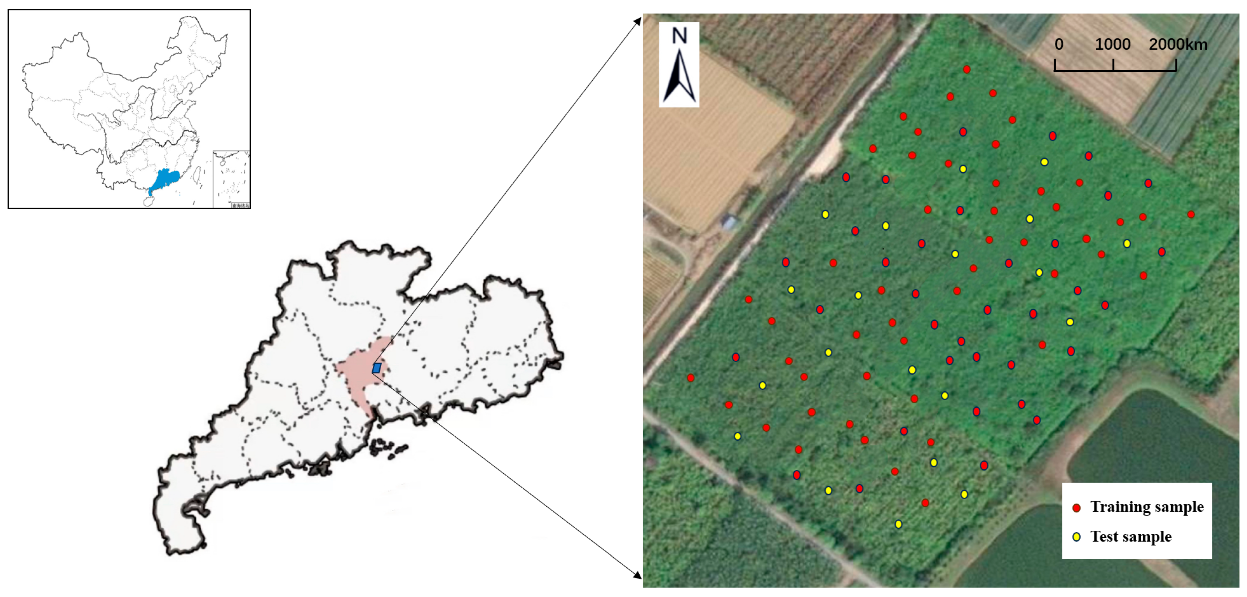
2.1. Study Area

The study area is located on the Pearl River Delta plain, with the flat agricultural fields of Guangzhou City, Guangdong Province (23°3′–23°18′ N, 112°55′–113°25′ E) selected as the research site. The Pearl River Delta is one of the most economically developed regions in China and serves as an important agricultural production base. The area experiences a subtropical monsoon climate (Cwa according to the Köppen-Geiger classification) [35], characterized by warm and humid conditions throughout the year. The average annual temperature in Guangzhou is approximately 21 °C, with annual precipitation typically ranging from 1600 to 2000 mm. The annual temperature and precipitation of Guangzhou in the Pearl River Delta in the recent 10 years are shown in Figure 1. These conditions provide ample water for crop growth. The rainy season, concentrated from April to September, brings abundant rainfall, which is particularly significant for agricultural activities, especially rice cultivation. Due to its low latitude, Guangzhou receives abundant sunshine, which is beneficial for photosynthesis and the growth and development of crops. The predominant soil type in the study area is red soil, classified as Acrisols according to the World Reference Base for Soil Resources (WRB) [36], and the farmland follows a crop-rotation system of wheat and maize, with two harvests per year [37]. This type of soil is commonly found in southern China, especially in humid subtropical regions. Red soil is rich in iron and aluminum but tends to be acidic, often requiring appropriate amendments to suit the growth of specific crops.

As an important city in the Pearl River Delta, Guangzhou’s agricultural development and land use are strongly influenced by urbanization. The changes in land use brought about by urbanization pose challenges to the local ecological environment and agricultural production models while also providing opportunities for agricultural technological innovation and sustainable development. These geographical and environmental characteristics make Guangzhou and its surrounding areas an ideal location for studying subtropical agricultural ecosystems and their adaptation strategies to climate change. Therefore, choosing Guangzhou as the study area is crucial.

2.2. Soil Sampling and Analysis

We collected surface soil samples from a depth of 0–20 cm in the farmland during the winter of 2022. All sampling points’ coordinates and elevations were recorded using a global navigation satellite system (GNSS), specifically the Haixingda GPS iRTK5X receiver (HaiXingDa Technology Co., Ltd., Nanjing, China), which supports both GPS and Beidou systems, along with relevant information such as slope position, aspect, farming practices, land use, and previous vegetation. As shown in Figure 2, 100 sampling points were randomly distributed in the FS experimental field. Each soil sample was tested for nitrate nitrogen (NO₃-N), pH, electrical conductivity (EC, μS/cm), and volumetric water content (%). Approximately 500 g of soil were collected from each sampling point, thoroughly mixed, and then placed in labeled plastic bags. In the laboratory, samples were air-dried, sieved through a 2 mm mesh, and homogenized. NO₃-N and pH were measured using the ion electrode method, while EC and VWC were determined using the frequency domain reflectometry (FDR) method [38,39,40,41]. The data were then organized, and outliers were handled.

Two experiments were conducted. First, the accuracy and effectiveness of three different interpolation methods—OK, RBF, and the newly proposed IDW-RBFNN framework (with parameters p = 1, 2, and 3)—were evaluated using the 100 samples. In this experiment, NO₃-N, pH, EC and VWC were set as the parameters. Second, to study the spatial variability of soil nutrient parameters under different sampling densities, we designed an experiment to progressively reduce the number of sampling points. This approach aimed to investigate the impact of sampling density on interpolation accuracy and determine the minimum acceptable sampling density under limited resources. As shown in Figure 1, 80 samples were randomly selected as the training set (red sample points) and 20 as the test set (yellow sample points) from the 100 samples. Subsequently, 40 samples were randomly selected from the 80 training samples, and then 20 samples from the 40. Ultimately, subsets of the training set (n = 80, 60, 40, and 20) were selected. We then analyzed the soil electrical conductivity using the OK, RBF, and IDW-RBFNN interpolation methods, creating four different sampling densities. The interpolation results for each density were evaluated using cross-validation.

Descriptive statistical variables, including minimum, maximum, mean, median, standard deviation, and coefficient of variation (CV), were calculated using the SPSS 24.0 software package. Exploratory statistical analysis was conducted using the geostatistical analysis module in ArcGIS 10.6, and the spatial interpolation maps of the parameters in this study were obtained using ArcMap 10.8.2 from the ArcGIS suite.

2.3. Spatial Interpolation Method

2.3.1. Ordinary Kriging (OK)

OK is a geostatistical interpolation method that leverages the spatial structure of data through a variogram model to minimize the estimation variance. It is particularly effective in capturing spatial autocorrelation and providing error estimates, making it suitable for complex spatial datasets [25,26,27]. However, OK’s effectiveness is highly dependent on the spatial distribution of data points and the accuracy of the variogram model, which requires careful selection and fitting. This dependence can lead to suboptimal predictions in regions with sparse or uneven data, as well as increased computational complexity [28,42].

2.3.2. Inverse Distance Weighting (IDW)

IDW is a straightforward interpolation technique that assigns weights to known points based on their distances to the point being estimated. Closer points have a larger influence on the interpolated value [17,20,21,43]. While IDW is effective in uniformly distributed datasets, it is sensitive to outliers and struggles with non-linear spatial variations, often leading to inaccurate predictions in areas with complex spatial patterns. This method also tends to produce poor results in boundary regions due to its reliance on the distance parameter [26,42].

2.3.3. Radial Basis Function (RBF)

The RBF method, often applied in neural networks, interpolates values by weighting input data with radial basis functions based on distance [3,12]. It is particularly effective when dealing with large sample sizes and irregular spatial distributions. However, the method is sensitive to the choice of basis functions and parameter settings, which can lead to overfitting and reduced robustness in heterogeneous datasets. Its deterministic nature means that it does not account for stochastic variability in spatial data, limiting its generalizability in complex spatial environments [13,17].

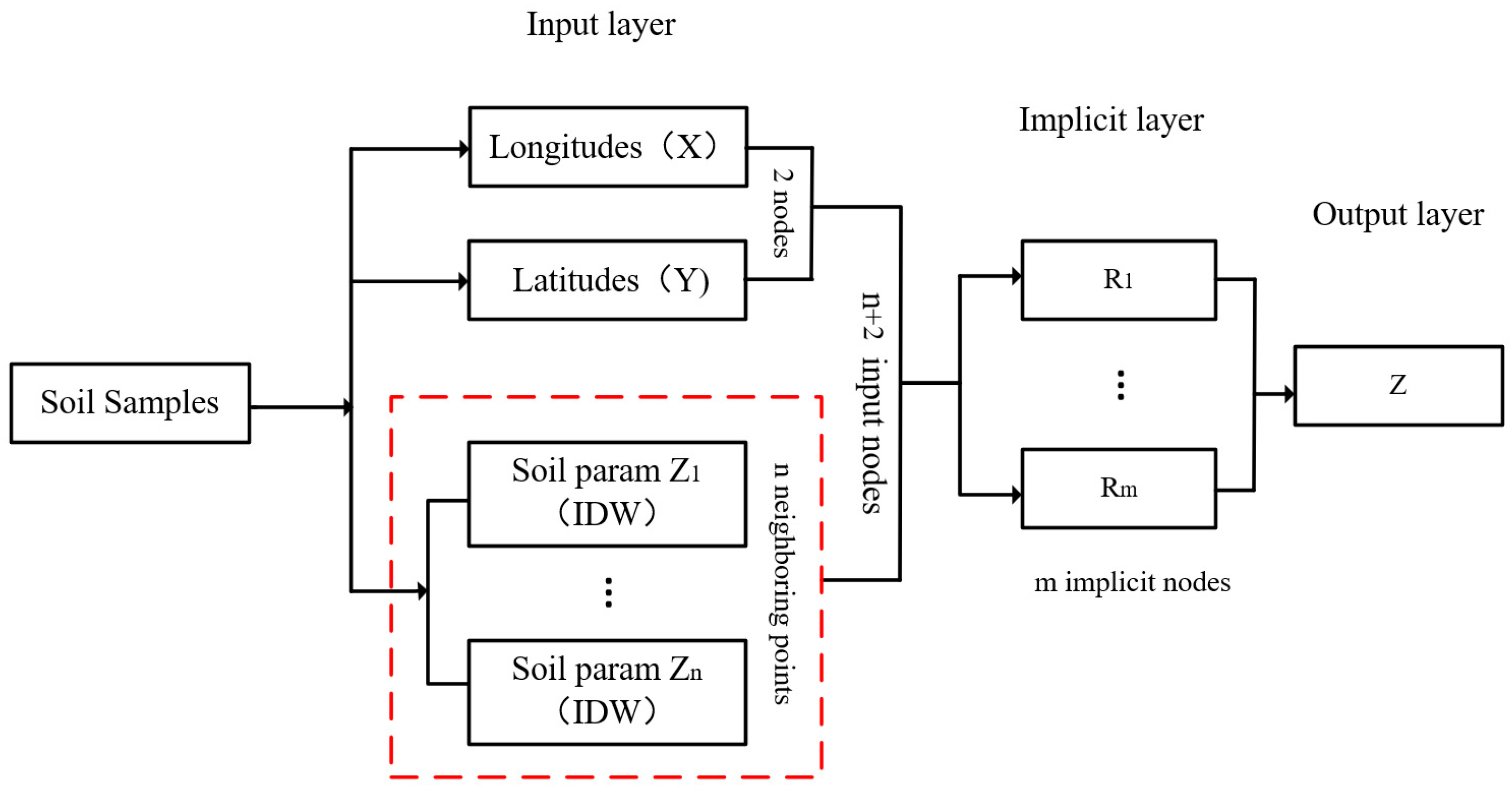
2.4. Detailed Design of the New Method

This study proposes an interpolation method based on a fusion of Radial Basis Function (RBF) neural networks and Inverse Distance Weighting (IDW) techniques, named IDW-RBFNN, to enhance the training effectiveness of the neural network. The research aims to provide more accurate soil parameter information for precise field fertilization.

First, before training the RBF neural network, we select n training sample points near the interpolation point and use the soil parameters of these points as n auxiliary variables, in addition to geographic coordinates. Next, the IDW method is applied to calculate the weight of each sample point: specifically, the distances from these n points to the interpolation point are calculated, and the inverse of these distances is raised to a power (which can be 1, 2, or 3) [27,44]. The sum of these inverse powers is used as a normalization factor. The weight of the soil parameters for each sample point is then the ratio of the inverse power of the distance to the sum. We then use the longitude, latitude, and the soil parameters of the n nearby points, processed through IDW, as input data, and the soil parameters of the interpolation point as output data to train the RBF neural network. After completing the network training, we can input the longitude and latitude coordinates of any location within the study area to obtain the soil parameters for that location. This method allows for the generation of an interpolation map of soil parameters for the entire study area.

As previously mentioned, incorporating IDW allows the input soil parameters to better reflect spatial distribution characteristics, enhancing the neural network’s learning capability. Choosing the IDW-RBFNN method significantly improves the accuracy and stability of soil parameter predictions. Therefore, we have decided to implement this method.

2.4.1. Generate RBFNN Interpolation Points

The Radial Basis Function Neural Network (RBFNN) is an artificial neural network that consists of an input layer, a hidden layer, and an output layer. The hidden layer nodes use Gaussian functions as the radial basis function (RBF) for activation, mapping the input data into a high-dimensional space, and the output is obtained through a linear combination of these functions [16,18]. RBFNN is used for handling nonlinear relationships and is a general-purpose machine learning model. It requires training to determine the centers and widths of the hidden nodes, as well as the weights of the output layer. It is important to note that the RBF interpolation method is different from RBFNN; the RBF interpolation function is determined by solving a linear system and does not involve a training process.

First, the geographical coordinates X, Y and soil parameters Z of all soil samples are input. The original samples are then randomly divided into training and validation samples. Next, Z-score normalization was applied to the training samples, validation samples, and interpolation samples to eliminate differences in the scales of different soil parameters (EC, NO₃-N, VWC, and pH), rescaling the data to have a mean of 0 and a standard deviation of 1. This ensures data consistency and stability during model training. Figure 3 demonstrates the spatial configuration of the study area, divided into a 100 × 100 grid, representing both the sampling and interpolation points across the research field. The red crosses mark the soil sampling points, which are the actual locations where soil data (such as geographic coordinates X, Y and soil parameters Z) were collected. These data serve as the inputs for training the Radial Basis Function Neural Network (RBFNN). By dividing the research area into a uniform grid, it ensures that the interpolation process can be systematically applied across the entire study region. The grid cell size is determined by the spatial resolution of the raster created during the interpolation process. This grid resolution ensures a balance between computational efficiency and interpolation accuracy, with the grid interval reflecting the spatial resolution required for uniform interpolation across the entire study area. Each grid cell provides a reference point where the values of soil parameters, which are not directly sampled, can be interpolated based on the influence of nearby sampling points. The division into grids ensures that the prediction of soil parameters using RBFNN and IDW methods is applied uniformly, allowing for a consistent and accurate estimation of soil characteristics at unsampled locations.

2.4.2. Calculate IDW Weights of Adjacent Points

At each interpolation point, the n = 5 nearest sampling points are selected, and the distance from each neighboring point to the interpolation point is calculated. The weight for each neighboring point is determined based on the inverse power of the distance, using the formula $w_i={\displaystyle \frac{1}{d_i^p}}$, where di is the distance from the neighboring point to the interpolation point and p is the power parameter (typically between 1 and 3). The weights are then normalized so that their sum equals 1, resulting in the weighted soil parameter value for each neighboring point.

2.4.3. Establish and Train IDW-RBFNN

A framework for the IDW-RBFNN neural network was established, with the input layer consisting of geographical coordinates X, Y and soil parameter values from five neighboring points. These values are obtained through inverse distance weighting, resulting in a total of seven input nodes. Z₁ (IDW) to Z_n (IDW) represent the inverse distance-weighted soil parameter values for the n neighboring points, with n set to 5 [17].

The hidden layer contains mmm nodes, which are used to extract features from the input geographical coordinates and soil parameters of the neighboring points and map these features to the output soil parameter values. The hidden nodes apply radial basis functions to perform a nonlinear transformation of the input data, helping the network capture the complex relationships between the input and output data. The features extracted by the hidden layer nodes R₁ to R_m are used to predict the soil parameter Z at the sampling points [27,42].

Finally, by training the RBF neural network, the nonlinear mapping relationship between the soil parameter Z and the n + 2 input nodes in the study area can be obtained and stored in the network (see Figure 4).

The choice of the exponent p in the Inverse Distance Weighting (IDW) method affects the rate at which the weight λi approaches zero. Typically, the value of p ranges from 1 to 3 [18,26]. Therefore, we set p to 1, 2, and 3, respectively. In each of these cases, we calculated the inverse distance-weighted values of the soil parameters for the five sampling points closest to the interpolation point out of 20 training samples. These weighted results, along with the geographical coordinates X and Y of the interpolation point, were used as the seven input nodes of the input layer, with the soil parameters of the interpolation point as the output, to train the RBFNN [42,43]. The parameter settings for the RBFNN are shown in

Table 1. RBFNN network parameter settings.

Parameter Name	Value	Description
Number of hidden neurons (mn)	2	Determined through calculation, reflects the ability to assimilate and absorb sample information
Spread	1	Default value
Display frequency (df)	25	Default value
Population size (NIND)	40	Population size in the genetic algorithm
Crossover probability (Pc)	0.7	Crossover probability in the genetic algorithm
Mutation probability (Pm)	0.1	Mutation probability in the genetic algorithm
Generations (MAXGEN)	200	Maximum number of iterations in the genetic algorithm

:

The genetic algorithm mentioned in Table 1 is a general optimization tool used in various interpolation methods like IDW, Kriging, and RBF-based models. In the IDW-RBFNN framework, it optimizes parameters such as weights, biases, and the spread of radial basis functions in the hidden layer. Acting as a global search strategy, it finds parameter combinations that minimize network error by generating and optimizing multiple “individuals” through crossover, mutation, and selection. This approach helps avoid local minima and improves the model’s ability to fit the data and enhance interpolation accuracy [34,43]. During the network training process, the weights and biases of the network are adjusted until the network converges and the error is minimized. The trained IDW-RBFNN neural network is then validated using the test samples to evaluate its prediction accuracy. The final trained IDW-RBFNN neural network model can accurately predict the soil parameter value Z′ at the interpolation point based on the input geographical coordinates X, Y and the soil parameters of the neighboring points.

2.5. Cross-Validation and Assessment

Cross-validation techniques were used to evaluate and compare the performance of different interpolation methods. The sample points were randomly divided into two datasets: one for training the model and the other for validating it. To reduce variability, the training and validation sets must be rotated across consecutive rounds so that each data point can be validated. The predictive performance of different interpolation methods was assessed using several statistical metrics, including Root Mean Square Error (RMSE), Mean Relative Error (MRE), R-squared (R²), and Concordance Correlation Coefficient (CCC) [45]. The formulas for these metrics are defined as follows:

$$\mathrm{RMSE}=\sqrt{{\displaystyle \frac{1}{n}}\sum _{i=0}^n(t_{\mathrm{o}\mathrm{b}\mathrm{s}\mathrm{e}\mathrm{r}\mathrm{v}\mathrm{e}\mathrm{d}}-t_{\mathrm{p}\mathrm{r}\mathrm{e}\mathrm{d}\mathrm{i}\mathrm{c}\mathrm{t}\mathrm{e}\mathrm{d}}{)}^2}$$

$$\mathrm{MRE}={\displaystyle \frac{1}{n}}\sum _{i=0}^n\left|{\displaystyle \frac{t_{\mathrm{observed}}-t_{\mathrm{predicted}}}{t_{\mathrm{observed}}}}\right|$$

$$R^2=1-{\displaystyle \frac{\sum _{i=1}^n(t_{observed}-t_{predicted}{)}^2}{\sum _{i=1}^n(t_{observed}-{\overline{t}}_{observed}{)}^2}}$$

$$CCC={\displaystyle \frac{2\cdot \rho \cdot {\sigma }_t}{{\sigma }_t^2+{\sigma }_{t_{predicted}}^2+(t_{observed}-t_{predicted}{)}^2}}$$

where $t_{\mathrm{o}\mathrm{b}\mathrm{s}\mathrm{e}\mathrm{r}\mathrm{v}\mathrm{e}\mathrm{d}}$ represents the observed values, $t_{\mathrm{predicted}}$ represents the predicted values, n is the number of validation sample points, $\rho$ is the Pearson correlation coefficient, ${\sigma }_t$ is the standard deviation of the observed values, and $t_{observed}$ is the standard deviation of the predicted values. RMSE measures the average deviation between predicted and observed values, calculated as the square root of the average of squared differences, with smaller RMSE values indicating better model accuracy. MRE quantifies the relative error of predictions compared to actual observations, expressed as a percentage, providing insight into the predictive accuracy relative to the observed values. R-squared evaluates the proportion of variance in the dependent variable that can be explained by the independent variables, with values closer to 1 indicating a better fit. Finally, CCC assesses the agreement between predicted and observed values, emphasizing both correlation and consistency, with values ranging from −1 to 1, where values closer to 1 signify strong agreement [45].

3. Results

3.1. Soil Nutrient Parameter Data

The

Table 2. Statistical results of soil fertility parameter description.

Soi Parameter	Samples	Min	Max	Mean	S.D	C.V
EC (μS/cm)	80	125	464	293.21	97.86	0.334
NO3-N (mg/kg)	80	16	79	33.44	18.19	0.544
pH	80	4.36	5.18	4.83	0.237	0.049
VWC (%)	80	0.098	0.173	0.132	0.0217	0.164

Note: EC (Electrical Conductivity, μS/cm): Represents the soil’s ability to conduct electrical current, related to the concentration of soluble salts. NO₃-N (Nitrate Nitrogen, mg/kg): Indicates the amount of nitrate nitrogen in the soil, essential for plant growth. pH: Measures the acidity or alkalinity of the soil, which affects nutrient availability and plant health. VWC (Volumetric Water Content, %): Reflects the amount of water in the soil, crucial for evaluating soil moisture levels.

below presents the descriptive statistics for various soil parameters including EC, NO₃-N, pH, and VWC.

The EC has a minimum value of 125 µS/cm, a maximum value of 464 µS/cm, and an average of 293.21 µS/cm. The standard deviation is 97.86 µS/cm, with a coefficient of variation of 0.334. The NO₃-N concentration ranges from 16 to 79 mg/kg, with an average value of 33.44 mg/kg. The standard deviation is 18.19 mg/kg, and the coefficient of variation is 0.544. The VWC ranges from 0.098 to 0.173, with an average value of 0.132. The standard deviation is 0.0217, and the coefficient of variation is 0.164. The coefficient of variation (CV) reflects the uniformity and variability of nutrient parameters in farmland. The results indicate that NO₃-N in the samples has the highest relative variation, EC shows moderate variation, and VWC and pH have the lowest coefficients of variation, indicating the least dispersion in their data.

3.2. Accuracy Assessment of Different Interpolation Methods in Soil Parameters

The dataset was divided into two randomly selected yet spatially balanced subsets, with 80% used for training the model and 20% for testing. The differences between the observed and predicted values of soil parameters in the test dataset were used to evaluate the predictive accuracy of the different models (

Table 3. Cross-validation and assessment results of different interpolation methods.

Interpolation Methods		Cross-Validation and Assessment
			RMSE	MRE	R2	CCC
EC	OK		81.7	0.260	0.6247	0.5745
	RBF		77.3	0.267	0.7921	0.5415
		Power
		1	76.6	0.262	0.8165	0.6845
	IDW-RBFNN	2	74.9	0.242	0.713	0.7495
		3	77.0	0.259	0.684	0.5601
VWC	OK		0.0203	0.117	0.6235	0.7527
	RBF		0.0254	0.151	0.6988	0.7261
		Power
		1	0.0213	0.123	0.4219	0.6892
	IDW-RBFNN	2	0.0212	0.124	0.4743	0.6409
		3	0.0213	0.125	0.6051	0.7635
pH	OK		0.256	0.048	0.7652	0.6977
	RBF		0.322	0.056	0.6824	0.7587
		Power
		1	0.282	0.052	0.8351	0.7841
	IDW-RBFNN	2	0.264	0.046	0.7237	0.6892
		3	0.278	0.049	0.6775	0.4598
NO3-N	OK		10.68	0.320	0.7652	0.5219
	RBF		8.66	0.316	0.8524	0.6931
		Power
		1	7.47	0.242	0.6888	0.8954
	IDW-RBFNN	2	8.39	0.287	0.7471	0.7225
		3	8.44	0.304	0.4788	0.3654

). To identify the best interpolation method for monitoring the distribution of soil fertility parameters in farmland, we evaluated the accuracy of three interpolation methods: Ordinary Kriging (OK), Radial Basis Function (RBF), and Inverse Distance Weighting-Radial Basis Function Neural Network (IDW-RBFNN) with power parameters (p) of 1, 2, and 3.

For EC, it is clear that the IDW-RBFNN method with a power parameter of 2 performs the best, achieving optimal evaluations across three indicators: an RMSE of 74.9 μS/cm, an MRE of 0.242, and a CCC of 0.6495. Compared to the OK and RBF methods, IDW2-RBFNN demonstrates lower RMSE and higher CCC values, indicating its superior accuracy and reasonable consistency. In the estimation of VWC, the OK method is regarded as the best choice due to its lowest RMSE of 0.0203%, lowest MRE of 0.117, and relatively high R² of 0.6235 and CCC of 0.7527, which suggest higher accuracy and consistency in predictions compared to other methods. For pH, the IDW-RBFNN method with a power parameter of 1 achieves the best evaluation in two key indicators, with an R² of 0.8351 and a CCC of 0.7841. These high R² and CCC values indicate that the IDW-RBFNN method effectively captures and reflects variations in soil pH. Similarly, for NO₃-N, IDW-RBFNN method with power parameter 1 still performs best.

The evaluation results of interpolation methods indicates that no single method consistently outperforms the others across all parameters. The choice of method should depend on the specific parameter being estimated. OK is recommended for VWC, while IDW-RBFNN with a power parameter of 2 is optimal for EC, and IDW-RBFNN with a power parameter of 1 is best for NO₃-N and pH.

3.3. Evaluation of Interpolation Accuracy at Different Sampling Densities

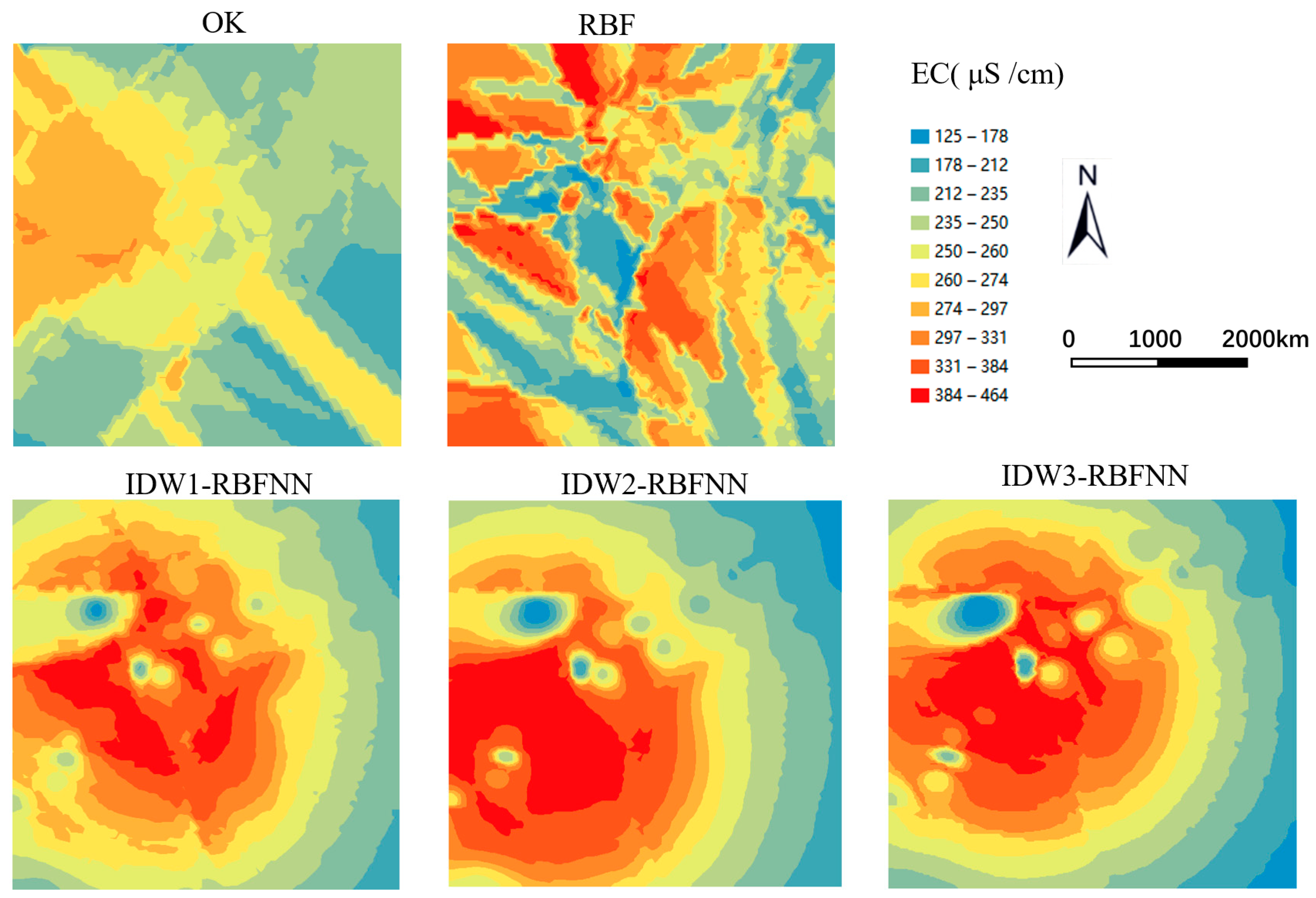
3.3.1. Soil EC Interpolation

Figure 5 illustrates the spatial distribution patterns of soil solution EC in farmland, obtained using different interpolation methods. The results from the OK interpolation show a smoother and more continuous variation in conductivity, with high conductivity areas confined to a smaller range. This smooth transition and lower spatial variability are attributed to the spatial autocorrelation modeling inherent in the OK method. However, OK interpolation has a higher RMSE (as shown in Table 3), indicating lower interpolation accuracy. This may be due to the statistical model of spatial continuity not fully matching the actual spatial heterogeneity of soil conductivity. Compared to the OK method, the RBF shows more intense color changes, with sharper conductivity variations and more scattered high-conductivity peaks, indicating more discontinuities. Its RMSE is lower than that of the OK method, suggesting that RBF has better accuracy in capturing complex spatial variability [18,20,27]. The IDW1-RBFNN interpolation exhibits moderate color changes, with smoother peaks and valleys compared to RBF. IDW2-RBFNN shows better spatial continuity, with more delicate color gradients and less sharp peaks than IDW1-RBFNN, indicating more concentrated high-conductivity areas and a more pronounced concentric pattern. This suggests higher spatial continuity and lower spatial variability, likely due to adjustments in IDW parameters (such as weight adjustments), resulting in less pronounced local changes. IDW3-RBFNN shows a very concentrated high-conductivity area, almost forming a single high-conductivity center, indicating the highest local data point weight, suggesting a higher degree of smoothing and less local variation. This indicates that further adjustments to the IDW parameters may have strengthened the consderation of distant data points, reducing local extremes [28,42].

EC reflects the concentration of dissolved salts in the soil and typically exhibits high spatial heterogeneity, especially under different agricultural practices, such as irrigation or fertilization [41]. EC is influenced not only by soil composition but also by factors like groundwater, surface runoff, and fertilization, which can create localized high-value regions [18]. The IDW-RBFNN method combines the local sensitivity of IDW’s weight allocation with the nonlinear learning capability of RBFNN. With a power parameter of p = 2, this method strikes a better balance between capturing local extremes and maintaining overall trends, allowing the interpolation to capture localized high values without introducing excessive smoothing. Given the significant local variability in EC data, using IDW-RBFNN with p = 2 can effectively handle pronounced local fluctuations, especially in cases where sample data is limited, by appropriately weighting local predictions for higher accuracy [19].

3.3.2. Soil NO₃-N Interpolation

Figure 6 shows the spatial distribution patterns of NO₃-N content in farmland soil obtained using different interpolation methods. The OK method presents relatively smooth interpolation results, with high nitrate nitrogen areas being concentrated and a general trend of gradual decrease from the center outward. This is because OK interpolation tends to balance surrounding sample points, reducing the influence of extreme values. In comparison, the RBF interpolation results show more dispersed high-value regions of nitrate nitrogen, characterized by sharper color changes and distinct regional boundaries. This is because RBF adjusts the basis function to fit the data, especially when there are significant changes in conductivity, potentially exaggerating local data differences [19]. The IDW1-RBFNN and IDW2-RBFNN methods provide relatively smooth interpolation results, indicating that lower inverse distance weights in these methods help balance the influence of neighboring points and maintain data continuity over a larger area. However, in IDW3-RBFNN, as the weight increases, the high nitrate nitrogen areas become exceptionally concentrated, revealing an intensified influence of local data points. This effect, while enhancing local precision, may also introduce problems of local overfitting, resulting in unnaturally concentrated spatial distributions [16,30,43].

NO₃-N is a common nitrogen form in agricultural soils, typically influenced by local factors such as fertilization, crop growth, rainfall, and soil drainage [38,46]. Due to the highly uneven spatial distribution of nitrogen fertilizers and plant uptake, NO₃-N often shows localized high-value regions and spatial clustering, with these high concentrations closely related to fertilized areas or specific farming practices. The spatial distribution of NO₃-N is characterized by significant local variability and heterogeneity. When using IDW-RBFNN with p = 1, the lower power parameter allows nearby sample points to have a greater influence on the interpolation results, effectively capturing localized extremes and high-concentration areas. This enables IDW-RBFNN to better reflect the clustering characteristics of NO₃-N, without excessively smoothing local variability, making it particularly suitable for parameters like NO₃-N that are strongly influenced by localized agricultural activities.

3.3.3. Soil pH Interpolation

Figure 7 displays the mapping results of soil solution pH in farmland using different interpolation methods. Visually, the OK interpolation method appears the smoothest, with gentle color transitions and no sharp changes or pronounced local extremes. The pH values gradually change from the center to the edges, indicating a central concentration trend [23,24,26]. Additionally, the OK method exhibits the lowest RMSE (Table 3), suggesting it is the most robust in fitting global data. In contrast, the Radial Basis Function (RBF) interpolation shows more pronounced spatial variability and discontinuity in local areas, with sharp pH changes and clear boundaries. This occurs because RBF, as a global interpolation method, fits the interpolation function using the entire dataset, even considering samples far from the interpolation points.

This method may lead to insensitivity to local data variations, resulting in sharp global changes, making its global consistency inferior to the OK method. Similarly, in the IDW-RBFNN series, when the weight p = 1, the results show good continuity, as the lower weight prevents the overall trend from being overly influenced by local extremes. As the inverse distance weight increases from p = 1 to 3, the high pH areas become more concentrated, causing the interpolation results to appear fragmented in local regions [23,24].

Soil pH reflects the acidity or alkalinity of the soil and is influenced by various factors, including soil parent material, vegetation, fertilization, and long-term rainfall [40]. While pH values may exhibit a generally smooth trend on a global scale, significant local fluctuations can occur, especially due to fertilization and soil treatment practices. These local fluctuations result in high heterogeneity and spatial differences in certain areas. IDW-RBFNN with p = 1 is better equipped to handle such local extremes and significant small-scale variations. By using a lower power parameter, IDW-RBFNN can capture these local variations effectively without over-smoothing the details, making it particularly well-suited for parameters like pH, which exhibit both global smoothness and significant localized variability [23,24].

3.3.4. Soil VWC Interpolation

Figure 8 illustrates the mapping results of soil VWC in farmland using different interpolation methods. The OK method exhibits smooth and continuous moisture transitions, with the main high-moisture areas confined to smaller regions. This ensures gradual moisture changes and relatively low spatial variability. This smoothness is mainly due to OK’s consideration of statistical correlation among sample points, resulting in natural fluctuations and continuity in the interpolation results. In contrast, the RBF method shows more pronounced moisture changes and a more dispersed distribution of peak values when applied to the same dataset. This is because the RBF method relies heavily on the configured basis function and its parameters (such as the shape parameter), which determine the function’s sensitivity to distance [28,42]. When the basis function is sensitive to variations within a small range, it can result in sharp moisture changes and the aggregation of high peak values in the spatial interpolation results. Within the IDW-RBFNN series, as the inverse distance weight increases (from 1 to 3), the interpolation results display more concentrated high-moisture areas and clearer concentric patterns. However, compared to the OK method, these results exhibit greater variability in overall spatial distribution. This increased variability occurs because the IDW-RBFNN method introduces a distance-based weighting mechanism when handling spatial relationships among points but does not employ a variogram function to describe the statistical correlation between sample points, as the OK method does [29]. As a result, IDW-RBFNN tends to emphasize the characteristics of local water content data points, overlooking the coherence of the overall spatial structure. This leads to less continuity and consistency in the spatial distribution, causing greater overall spatial variability.

VWC measures the water content in the soil and usually displays a more continuous spatial variation. VWC is heavily influenced by climate factors (such as rainfall) and soil structure, but these effects often manifest as smooth spatial gradients over larger scales, rather than abrupt local extremes. Therefore, the spatial distribution of VWC is generally smoother and less subject to the significant local fluctuations seen in EC. Ordinary Kriging (OK) uses a variogram to model spatial autocorrelation, making it well-suited for capturing the global smooth trends present in VWC. By accounting for statistical correlations among sample points, OK provides reliable global interpolation, especially for parameters like VWC that exhibit gradual spatial changes. Thus, OK can effectively capture the overall trends and variations in VWC without relying on localized extremes.

3.4. Evaluation of Interpolation Accuracy at Different Sampling Densities

We conducted an experiment with gradually decreasing sampling points to study and analyze the impact of different sampling densities on the effectiveness of interpolation methods. This helps us evaluate their performance in situations where data is incomplete or sampling density is insufficient. We used k-fold cross-validation with k = 5, ensuring that each fold contained a representative sample of the full dataset. The test sets were randomly selected for each iteration, and the cross-validation process was repeated three times to ensure that the results were not biased by any particular partition of the data. Taking soil conductivity as an example, the cross-validation results for the interpolation methods OK, RBF, and IDW-RBFNN (with p = 1, 2, 3) under four different sampling densities are shown in

Table 4. The cross-validation results of different interpolation methods under four sample densities.

EC		Cross-Validation
	Samples	80		60		40		20
Method		RMSE	MRE	RMSE	MRE	RMSE	MRE	RMSE	MRE
OK		0.099	0.127	0.105	0.137	0.130	0.169	0.214	0.276
RBF		0.108	0.140	0.119	0.161	0.140	0.185	0.191	0.262
	Power
	1	0.104	0.132	0.103	0.136	0.130	0.165	0.187	0.257
IDW-RBFNN	2	0.102	0.133	0.098	0.127	0.145	0.183	0.194	0.267
	3	0.099	0.129	0.102	0.129	0.151	0.189	0.211	0.288

. In the evaluation of interpolation methods, OK consistently achieved the lowest Root RMSE of 0.099 and a MRE of 0.127 when utilizing a sample size of 80, indicating a high level of accuracy. When the sample size was reduced to 60, the IDW-RBFNN series (p = 2) exhibited commendable performance, achieving minimum RMSE and MRE values of 0.098 and 0.127, respectively. For smaller sample sizes of 40 and 20, the IDW1-RBFNN method delivered the best results, with RMSE values of 0.130 (n = 40) and 0.187 (n = 20), accompanied by MRE values of 0.165 (n = 40) and 0.257 (n = 20). The analysis indicates that the RMSE (Root Mean Square Error) and MRE (Mean Relative Error) of the different interpolation methods increase as the number of training samples decreases, suggesting that more sampling points can improve interpolation accuracy. When the sample size reaches 60, the accuracy of EC interpolation is at its highest.

4. Discussion

4.1. Comparison of Different Interpolation Methods

The choice of different interpolation parameters for the same interpolation method can significantly affect interpolation accuracy. To minimize errors, comparisons among different interpolation methods should be based on optimal parameters. In our study, we compared the IDW-RBFNN (with powers of 1, 2, and 3), OK, and RBF methods.

The results indicate that the IDW-RBFNN method showed the highest interpolation accuracy for soil parameter content across various parameters, followed by OK, while RBF exhibited the lowest accuracy (Table 3). The RBF method demonstrated higher RMSE and MRE values across all sampling densities, indicating consistently poorer interpolation performance [47]. This is largely due to the nature of RBF as a global interpolation method, which struggles to effectively manage local heterogeneity compared to OK and IDW-RBFNN. RBF is better suited for larger sample sizes and smoother surface variations. Furthermore, RBF requires fewer adjustable parameters, primarily the type of radial basis function and parameters (such as the width of the Gaussian function), making the parameter selection process relatively simple and requiring less optimization and adjustment [48,49]. Additionally, it necessitates fewer data preprocessing steps and imposes fewer strict assumptions and tests. Thus, RBF can be considered when the sample size is sufficiently large. In contrast, the OK interpolation method requires statistical testing, normal transformations, spatial structure analysis, and semivariogram fitting prior to interpolation, making it more complex to implement. It accounts for sample location, distance relationships, and spatial structures, which makes it less influenced by sample density and quantity. Consequently, it is theoretically the optimal estimation method. However, when the sample size is minimal (20), the OK method is significantly affected, with RMSE and MRE reaching 0.214 and 0.276, respectively (Table 3), resulting in lower interpolation accuracy than other methods. Similarly, the IDW-RBFNN method combines the characteristics of Inverse IDW and RBF, leading to more complex calculations and a greater number of parameters, such as the power parameter (P), which can influence the interpolation results [44]. Compared to OK and RBF methods, this requires more experimentation and adjustments. It is important to note that no single interpolation method is suitable for all regions; optimal interpolation parameters can only be determined through repeated exploratory experiments. Despite the increased complexity of the IDW-RBFNN method, its accuracy advantage at lower sampling densities makes it a viable option worth considering.

4.2. Identification of Optimal Sampling Number for Spatial Distribution

In theory, interpolation accuracy tends to improve with an increasing number of samples [29,30]. However, once the sample size reaches a certain threshold, the accuracy plateaus, and the marginal gains in accuracy become limited. Additionally, redundancy in the data is inevitable, which incurs higher costs and longer processing times. Therefore, it is essential to determine a reasonable number of sampling points. In this study, when the number of sampling points was reduced from 80 to 60, the RMSE and MRE values of IDW2-RBFNN decreased (Table 3). This is attributed to the minimal variation in the physical and chemical properties of the soil within the same category. When 60 sample points are evenly distributed across these characteristic areas, the IDW-RBFNN model can more accurately capture changes in electrical conductivity. Conversely, when the sample size increases to 80, newly added points may fall in areas with significant fluctuations in conductivity, potentially leading to decreased interpolation accuracy. Moreover, a larger sample size may introduce extreme or outlier values (e.g., contaminated soil samples or those with differing fertilization histories), which can distort the overall dataset and impact the accuracy of the interpolation model [1,30,49]. Considering the trade-offs between interpolation accuracy and resource limitations, we recommend utilizing the IDW-RBFNN method (p = 2) with 60 samples as the minimum sampling density to ensure high interpolation accuracy even under constrained resources. It is important to note that the optimal interpolation method and sample size proposed in this study are the best configurations under the specific conditions set forth in this paper, and there may be more effective configurations. When employing spatial interpolation methods, it is crucial to thoroughly analyze the sample data and repeatedly test and compare various interpolation techniques and parameters tailored to the specific context of the study area to achieve the best spatial interpolation results.

5. Conclusions

This study presents an interpolation prediction framework that combines the Radial Basis Function (RBF) neural network with Inverse Distance Weighting (IDW), referred to as IDW-RBFNN. Essentially, IDW-RBFNN is a variant of the RBF method. Specifically, IDW-RBFNN integrates the spatial data interpolation advantages of IDW with the RBF neural network’s ability to handle complex nonlinear relationships, thus creating a novel interpolation prediction framework.

IDW-RBFNN consistently maintains a low error rate in most cases, depending on different power value (p) settings, even with a fixed number of data samples. The IDW-RBFNN method demonstrates the highest interpolation accuracy for EC, NO₃-N, and pH across various parameters, while the OK method provides optimal accuracy for VWC. Notably, in conditions of low sampling density for soil EC, the interpolation accuracy of OK is significantly affected, whereas IDW-RBFNN maintains relatively low error rates.

Considering interpolation accuracy and resource constraints, we recommend employing the IDW-RBFNN method (p = 2) with 60 samples as the minimum sampling density to ensure high interpolation accuracy under limited resources. Due to the absence of a universally optimal spatial interpolation method applicable to all situations, it is essential to identify the best interpolation methods and sampling numbers for different regions. This approach aids in determining the optimal sampling strategy under resource limitations, reveals the sensitivity of various interpolation methods to data sparsity and heterogeneity, and provides an effective tool for monitoring soil fertility in delta regions.

In practical applications, the IDW-RBFNN method has significant potential in precision agriculture, where it can optimize fertilizer application and irrigation practices by providing more accurate soil condition predictions at unsampled locations. Furthermore, by integrating this method with remote sensing data, such as UAVs or satellite sensors, real-time soil condition maps could be generated to enhance resource management and reduce environmental impacts.

Statement: The proposed IDW-RBFNN framework enhances the productive and environmental sustainability of farmers in the study region by providing more accurate spatial interpolation of soil parameters. This allows for precise management of soil fertility, which is crucial for optimizing crop yields and reducing the use of chemical inputs such as fertilizers. By improving the prediction accuracy of soil properties like NO₃-N, EC, pH, and VWC, the framework enables farmers to apply resources more efficiently, minimizing environmental impacts such as nutrient runoff and soil degradation. Ultimately, this contributes to more sustainable agricultural practices and supports the long-term viability of farming in the Pearl River Delta region.

References

1. Bhunia, G.S.; Shit, P.K.; Maiti, R. Comparison of GIS-based interpolation methods for spatial distribution of soil organic carbon (SOC). J. Saudi Soc. Agric. Sci. 2018, 17, 114–126. [Google Scholar] [CrossRef]
2. Chen, T.; Chang, Q.; Liu, J.; Clevers, J.G.; Kooistra, L. Identification of soil heavy metal sources and improvement in spatial mapping based on soil spectral information: A case study in northwest China. Sci. Total Environ. 2016, 565, 155–164. [Google Scholar] [CrossRef] [PubMed]
3. Chen, S.; Cowan, C.F.; Grant, P.M. Orthogonal least squares learning algorithm for radial. IEEE Trans. Neural Netw. 1991, 2, 302–309. [Google Scholar] [CrossRef] [PubMed]
4. Cambardella, C.A.; Moorman, T.B.; Novak, J.M.; Parkin, T.B.; Karlen, D.L.; Turco, R.F.; Konopka, A.E. Field-scale variability of soil properties in central Iowa soils. Soil Sci. Soc. Am. J. 1994, 58, 1501–1511. [Google Scholar] [CrossRef]
5. Hengl, T.; Heuvelink, G.B.; Stein, A. A generic framework for spatial prediction of soil variables based on regression-kriging. Geoderma 2004, 120, 75–93. [Google Scholar] [CrossRef]
6. Ajaj, Q.M.; Shareef, M.A.; Hassan, N.D.; Hasan, S.F.; Noori, A.M. GIS based spatial modeling to mapping and estimation relative risk of different diseases using inverse distance weighting (IDW) interpolation algorithm and evidential belief function (EBF) (Case study: Minor Part of Kirkuk City, Iraq). Int. J. Eng. Technol. 2018, 7, 185–191. [Google Scholar] [CrossRef]
7. Qiao, P.; Lei, M.; Yang, S.; Yang, J.; Guo, G.; Zhou, X. Comparing ordinary kriging and inverse distance weighting for soil as pollution in Beijing. Environ. Sci. Pollut. Res. 2018, 25, 15597–15608. [Google Scholar] [CrossRef]
8. Banuelos, G.S.; Ajwa, H.A. Trace elements in soils and plants: An overview. J. Environ. Sci. Health Part A 1999, 34, 951–974. [Google Scholar] [CrossRef]
9. Chai, X.; Shen, C.; Yuan, X.; Huang, Y. Spatial prediction of soil organic matter in the presence of different external trends with REML-EBLUP. Geoderma 2008, 148, 159–166. [Google Scholar] [CrossRef]
10. Godinho, S.; Guiomar, N.; Gil, A. Using a stochastic gradient boosting algorithm to analyse the effectiveness of Landsat 8 data for montado land cover mapping: Application in southern Portugal. Int. J. Appl. Earth Obs. Geoinf. 2016, 49, 151–162. [Google Scholar] [CrossRef]
11. Guo, P.T.; Li, M.F.; Luo, W.; Tang, Q.F.; Liu, Z.W.; Lin, Z.M. Digital mapping of soil organic matter for rubber plantation at regional scale: An application of random forest plus residuals kriging approach. Geoderma 2015, 237, 49–59. [Google Scholar] [CrossRef]
12. Liu, S.; Zhang, Y.; Ma, P.; Lu, B.; Su, H. A novel spatial interpolation method based on the integrated RBF neural network. Procedia Environ. Sci. 2011, 10, 568–575. [Google Scholar] [CrossRef]
13. Lin, G.F.; Chen, L.H. A spatial interpolation method based on radial basis function networks incorporating a semivariogram model. J. Hydrol. 2004, 288, 288–298. [Google Scholar] [CrossRef]
14. Imanian, H.; Shirkhani, H.; Mohammadian, A.; Hiedra Cobo, J.; Payeur, P. Spatial interpolation of soil temperature and water content in the land-water interface using artificial intelligence. Water 2023, 15, 473. [Google Scholar] [CrossRef]
15. Xie, M.J.; Wang, Y.; Kang, Y.; Wu, Z.T.; Chen, Q.L.; Liu, Q.; Wu, C.Y.; Zhang, J.M. Accuracy study of spatial predicting in soil attributes based on interpolations by artificial neural network and ordinary kriging. J. Ecol. Rural. Environ. 2021, 37, 934–942. [Google Scholar]
16. Qi, Q.; Yue, X.; Duo, X.; Xu, Z.; Li, Z. Spatial prediction of soil organic carbon in coal mining subsidence areas based on RBF neural network. Int. J. Coal Sci. Technol. 2023, 10, 30. [Google Scholar] [CrossRef]
17. Sheng, J.; Yu, P.; Zhang, H.; Wang, Z. Spatial variability of soil Cd content based on IDW and RBF in Fujiang River, Mianyang, China. J. Soils Sediments 2021, 21, 419–429. [Google Scholar] [CrossRef]
18. Baradaran Motie, J.; Aghkhani, M.H.; Rohani, A.; Lakziyan, A. Modeling the Effective Parameters on Accuracy of Soil Electrical Conductivity Measurement Systems Using RBF Neural Network. J. Agric. Mach. 2019, 9, 139–154. [Google Scholar]
19. Shahinzadeh, N.; Babaeinejad, T.; Mohsenifar, K.; Ghanavati, N. Spatial variability of soil properties determined by the interpolation methods in the agricultural lands. Model. Earth Syst. Environ. 2022, 8, 4897–4907. [Google Scholar] [CrossRef]
20. Bel-Lahbib, S.; Ibno Namr, K.; Rerhou, B.; Mosseddaq, F.; El Bourhrami, B.; Moughli, L. Assessment of soil quality by modeling soil quality index and mapping soil parameters using IDW interpolation in Moroccan semi-arid. Model. Earth Syst. Environ. 2023, 9, 4135–4153. [Google Scholar] [CrossRef]
21. Yadav, R.; Bhat, M.I.; Faisul-Ur-Rasool, P.K.; Ahmad, R.; Bisati, I.A.; Bhat, K.A.; Singh, R. Spatial distribution of soil physico-chemical properties of North Western Himalayan Region of Jammu and Kashmir, (India) using inverse distance weighted (IDW) interpolation technique in GIS environment. Agric. Machenization Asia 2022, 53, 8113–8124. [Google Scholar]
22. Robinson, T.P.; Metternicht, G. Testing the performance of spatial interpolation techniques for mapping soil properties. Comput. Electron. Agric. 2006, 50, 97–108. [Google Scholar] [CrossRef]
23. Emadi, M.; Baghernejad, M. Comparison of spatial interpolation techniques for mapping soil pH and salinity in agricultural coastal areas, northern Iran. Arch. Agron. Soil Sci. 2014, 60, 1315–1327. [Google Scholar] [CrossRef]
24. Staugaitis, G.; Šumskis, D. Spatial variability of soil pH as influenced by different soil sampling methods and geostatistical techniques. Zemdirb.-Agric. 2011, 98, 323–332. [Google Scholar]
25. Mondal, A.; Khare, D.; Kundu, S.; Mondal, S.; Mukherjee, S.; Mukhopadhyay, A. Spatial soil organic carbon (SOC) prediction by regression kriging using remote sensing data. Egypt. J. Remote Sens. Space Sci. 2017, 20, 61–70. [Google Scholar] [CrossRef]
26. Sun, Y.; Kang, S.; Li, F.; Zhang, L. Comparison of interpolation methods for depth to groundwater and its temporal and spatial variations in the Minqin oasis of northwest China. Environ. Model. Softw. 2009, 24, 1163–1170. [Google Scholar] [CrossRef]
27. Karydas, C.G.; Gitas, I.Z.; Koutsogiannaki, E.; Lydakis-Simantiris, N.; Silleos, G.N. Evaluation of spatial interpolation techniques for mapping agricultural topsoil properties in Crete. EARSeL Eproceedings 2009, 8, 26–39. [Google Scholar]
28. Dai, F.; Zhou, Q.; Lv, Z.; Wang, X.; Liu, G. Spatial prediction of soil organic matter content integrating artificial neural network and ordinary kriging in Tibetan Plateau. Ecol. Indic. 2014, 45, 184–194. [Google Scholar] [CrossRef]
29. Wen, L.; Zhang, L.; Bai, J.; Wang, Y.; Wei, Z.; Liu, H. Optimizing spatial interpolation method and sampling number for predicting cadmium distribution in the largest shallow lake of North China. Chemosphere 2022, 309, 136789. [Google Scholar] [CrossRef]
30. Shen, Q.; Wang, Y.; Wang, X.; Liu, X.; Zhang, X.; Zhang, S. Comparing interpolation methods to predict soil total phosphorus in the Mollisol area of Northeast China. Catena 2019, 174, 59–72. [Google Scholar] [CrossRef]
31. Fan, X.; Fan, N.; Qin, C.Z.; Zhao, F.H.; Zhu, L.J.; Zhu, A.X. Large-area soil mapping based on environmental similarity with adaptive consideration of spatial distance to samples. Geoderma 2023, 439, 116683. [Google Scholar] [CrossRef]
32. Ju, L.; Guo, S.; Ruan, X.; Wang, Y. Improving the mapping accuracy of soil heavy metals through an adaptive multi-fidelity interpolation method. Environ. Pollut. 2023, 330, 121827. [Google Scholar] [CrossRef] [PubMed]
33. Silatsa, F.B.; Yemefack, M.; Tabi, F.O.; Heuvelink, G.B.; Leenaars, J.G. Assessing countrywide soil organic carbon stock using hybrid machine learning modelling and legacy soil data in Cameroon. Geoderma 2020, 367, 114260. [Google Scholar] [CrossRef]
34. Yin, G.; Chen, X.; Zhu, H.; Chen, Z.; Su, C.; He, Z.; Qiu, J.; Wang, T. A novel interpolation method to predict soil heavy metals based on a genetic algorithm and neural network model. Sci. Total Environ. 2022, 825, 153948. [Google Scholar] [CrossRef]
35. Kottek, M.; Grieser, J.; Beck, C.; Rudolf, B.; Rubel, F. World Map of the Köppen-Geiger Climate Classification Updated. Meteorologische Zeitschrift. 2006. Available online: https://en.wikipedia.org/wiki/K%C3%B6ppen_climate_classification (accessed on 19 October 2024).
36. Food and Agriculture Organization of the United Nations (FAO). World Reference Base for Soil Resources 2014: International Soil Classification System for Naming Soils and Creating Legends for Soil Maps; World Soil Resources Reports No. 106; FAO: Rome, Italy, 2014; Available online: http://www.fao.org/soils-portal/soil-survey/soil-classification/world-reference-base/en/ (accessed on 19 October 2024).
37. Fotheringham. World Reference Base for Soil Resources; ISSSISRIC-FAO, FAO: Rome, Italy; Available online: https://www.fao.org/soils-portal/data-hub/soil-classification/world-reference-base/en/ (accessed on 19 October 2024).
38. Ward, R.C. NO3-N Soil Test—Approaches to use and interpretation. Commun. Soil Sci. Plant Anal. 1971, 2, 61–71. [Google Scholar] [CrossRef]
39. Wan, A.W.; Gray, M.N.; Graham, J. On the relations of suction, moisture content and soil structure in compacted clays. In Proceedings of the 1st International Conference on Unsaturated Soils, Paris, France, 6–8 September 1995; Volume 1, pp. 215–222. [Google Scholar]
40. Thomas, G.W. Soil pH and soil acidity. In Methods of Soil Analysis: Part 3 Chemical Methods; John Wiley & Sons, Inc.: Hoboken, NJ, USA, 1996; Volume 5, pp. 475–490. [Google Scholar]
41. Corwin, D.L.; Lesch, S.M. Apparent soil electrical conductivity measurements in agriculture. Comput. Electron. Agric. 2005, 46, 11–43. [Google Scholar] [CrossRef]
42. Mueller, T.G.; Pusuluri, N.B.; Mathias, K.K.; Cornelius, P.L.; Barnhisel, R.I.; Shearer, S.A. Map quality for ordinary kriging and inverse distance weighted interpolation. Soil Sci. Soc. Am. J. 2004, 68, 2042–2047. [Google Scholar] [CrossRef]
43. Chen, J.; Han, C.; Peng, Y.; Wang, M.; Zhao, Y. Improved three-dimensional mapping of soil chromium pollution with sparse borehole data: Incorporating multisource auxiliary data into IDW-based interpolation. Soil Use Manag. 2023, 39, 933–947. [Google Scholar] [CrossRef]
44. Ding, Q.; Wang, Y.; Zhuang, D. Comparison of the common spatial interpolation methods used to analyze potentially toxic elements surrounding mining regions. J. Environ. Manag. 2018, 212, 23–31. [Google Scholar] [CrossRef]
45. Lin, L.I.K. A concordance correlation coefficient to evaluate reproducibility. Biometrics 1989, 45, 255–268. [Google Scholar] [CrossRef]
46. Wang, Y.; Zhang, X.; Huang, C. Spatial variability of soil total nitrogen and soil total phosphorus under different land uses in a small watershed on the Loess Plateau, China. Geoderma 2009, 150, 141–149. [Google Scholar] [CrossRef]
47. Tziachris, P.; Aschonitis, V.; Chatzistathis, T.; Papadopoulou, M. Assessment of spatial hybrid methods for predicting soil organic matter using DEM derivatives and soil parameters. Catena 2019, 174, 206–216. [Google Scholar] [CrossRef]
48. Fazeli Sangani, M.; Namdar Khojasteh, D.; Owens, G. Dataset characteristics influence the performance of different interpolation methods for soil salinity spatial maping. Environ. Monit. Assess. 2019, 191, 684. [Google Scholar] [CrossRef] [PubMed]
49. Bronowicka-Mielniczuk, U.; Mielniczuk, J. New indices to quantify patterns of relative errors produced by spatial interpolation models–A comparative study by modelling soil properties. Ecol. Indic. 2023, 154, 110551. [Google Scholar] [CrossRef]
Figure 1. Annual temperature and precipitation in Guangzhou, Pearl River Delta.
Agronomy 14 02469 g001
Figure 2. Distribution of soil sampling in farmland.
Agronomy 14 02469 g002
Figure 3. Grid diagram of the research area.
Agronomy 14 02469 g003
Figure 4. The flowchart of the IDW-RBFNN interpolation framework. The red rectangle highlights the subset of input nodes in the IDW-RBFNN framework that are derived from the soil parameters of the five nearest neighboring points, obtained using the Inverse Distance Weighting (IDW) method.
Agronomy 14 02469 g004
Figure 5. Mapping results of soil solution EC using different interpolation methods.
Agronomy 14 02469 g005
Figure 6. Mapping results of soil NO3-N using different interpolation methods.
Agronomy 14 02469 g006
Figure 7. Mapping results of soil PH using different interpolation methods.
Agronomy 14 02469 g007
Figure 8. Mapping results of soil VWC using different interpolation methods.
Agronomy 14 02469 g008