Comparing Laboratory and Satellite Hyperspectral Predictions of Soil Organic Carbon in Farmland

Abstract

Mapping soil organic carbon (SOC) accurately is essential for sustainable soil resource management. Hyperspectral data, a vital tool for SOC mapping, is obtained through both laboratory and satellite-based sources. While laboratory data is limited to sample point monitoring, satellite hyperspectral imagery covers entire regions, albeit susceptible to external environmental interference. This study, conducted in the Yuncheng Basin of the Yellow River Basin, compared the predictive accuracy of laboratory hyperspectral data (ASD FieldSpec4) and GF-5 satellite hyperspectral imagery for SOC mapping. Leveraging fractional order derivatives (FODs), various denoising methods, feature band selection, and the Random Forest model, the research revealed that laboratory hyperspectral data outperform satellite data in predicting SOC. FOD processing enhanced spectral information, and discrete wavelet transform (DWT) proved effective for GF-5 satellite imagery denoising. Stability competitive adaptive re-weighted sampling (sCARS) emerged as the optimal feature band selection algorithm. The 0.6FOD-sCARS RF model was identified as the optimal laboratory hyperspectral prediction model for SOC, while the 0.8FOD-DWT-sCARS RF model was deemed optimal for satellite hyperspectral prediction. This research, offering insights into farmland soil quality monitoring and strategies for sustainable soil use, holds significance for enhancing agricultural production efficiency.

1. Introduction

Soil organic carbon (SOC) serves as the largest terrestrial carbon store, approximately three times the size of the vegetation carbon pool and twice that of the atmospheric carbon pool, playing a pivotal role in terrestrial ecosystems [1]. Minor variations in SOC storage can lead to significant fluctuations in atmospheric CO₂, impacting global climate [2,3]. Additionally, SOC serves as a crucial indicator of soil quality, vital for enhancing soil fertility, maintaining soil biodiversity, and improving plant productivity [4]. Accurate and efficient estimation and monitoring of SOC changes are crucial for predicting global climate change, simulating carbon cycles, and developing precision agriculture.

Numerous studies have estimated SOC spatial distribution at regional, national, and global scales [5,6]. Traditional soil mapping methods rely on discrete soil field survey points, which is challenging, time-consuming, and expensive [7]. Digital soil mapping (DSM), utilizing mathematical models based on soil data and environmental factors, infers spatiotemporal changes in soil properties [8]. Proximal hyperspectral technology, particularly visible and near-infrared (vis-NIR) spectroscopy, has become a significant data source for DSM, providing a practical and economical method for rapid and accurate soil property estimation [5,9]. Although studies mostly occur under laboratory conditions due to the higher estimation accuracy of laboratory spectral data, discrete soil samples provide limited point-to-point data [10].

In recent years, airborne hyperspectral imagery and satellite hyperspectral data have become powerful tools in DSM, allowing high-resolution, continuous soil mapping, reducing errors caused by spatial interpolation [11]. Using hyperspectral satellite data for large-scale soil property estimation and mapping holds great potential [12]. The visible shortwave infrared hyperspectral camera carried by the GF-5 satellite can capture spectra ranging from visible light to shortwave infrared (400–2500 nm). It is the world’s first hyperspectral camera that simultaneously covers a wide area and a broad spectral range. The camera comprises 330 spectral channels, offering a color range nearly nine times wider than conventional cameras. This configuration provides excellent potential for quantitative inversion applications. However, few studies have compared the performance of laboratory vis-NIR and satellite hyperspectral data in estimating surface SOC. Soil spectral reflectance significantly correlates with SOC, with hyperspectral data detecting finer SOC differences than multispectral data [12]. Mathematical transformations, such as fractional-order derivatives, can enhance SOC prediction accuracy, compensating for the shortcomings of integer–order derivative transformations like first-order derivative and second-order derivative methods [13]. Satellite hyperspectral data, subject to noise, require different denoising methods to improve SOC prediction accuracy [14].

Simultaneously, both laboratory hyperspectral data and satellite hyperspectral data face challenges of data redundancy and multicollinearity among hyperspectral bands, affecting SOC prediction effectiveness [15,16]. Feature band selection methods, such as variable importance projection (VIP), competitive adaptive re-weighted sampling (CARS), stability CARS (sCARS), and successive projections algorithm (SPA) can filter ineffective and redundant bands from full-spectrum data, enhancing overall prediction accuracy when using hyperspectral data to predict and map surface soil SOC.

This study aimed to (1) process satellite hyperspectral data (GF-5 satellite imagery) with different denoising treatments and compare the potential of laboratory and satellite hyperspectral data in predicting agricultural SOC; (2) evaluate and compare the ability of feature selection techniques in enhancing the accuracy of SOC prediction models; (3) identify the best method for satellite hyperspectral prediction of SOC and map SOC spatial variability.

2. Materials and Methods

2.1. Study Area

The study area is situated in Yuncheng City, Shanxi Province, China (Figure 1, 110.34°–110.55° E, 34.92°–35.59° N), within the Yuncheng Basin in the middle reaches of the Yellow River Basin. The region encompasses a mix of mountainous and hilly terrain. Covering an approximate area of 5304.74 km², equivalent to the size of a single GF-5 satellite image (Figure 2), the study area features diverse agricultural land types, including dry land, irrigated land, and sloping cultivated land (terraces), totaling about 4776.34 km². Bordered by the Yellow and Fen rivers, the predominant soil type in this region is Cambisols, consistent with World Reference Base for soil resources (WRB). The area witnesses distinct seasonal variations: limited rain and snow in winter, minimal rainfall in spring, hot and rainy conditions in summer, and rapid cooling in autumn. The average annual temperature stands at 12.5 °C, with annual rainfall ranging from 520 to 550 mm.

2.2. Soil Sample Collection and Processing

Between 2018 and 2021, we established 312 soil sample points, ensuring a uniform distribution across agricultural plots. At each sampling point, three surface soil samples were collected within a 20 m × 20 m grid and then combined. Using a portable GPS device (GPS, G350, UniStrong, Beijing, China), we recorded the geographical coordinates of each sample. Careful measures were taken to remove impurities from the soil surface during sampling. The collected soil samples were sealed in plastic bags to prevent moisture evaporation and transported to the laboratory for air drying, grinding, and sieving. The SOC content was determined using the potassium dichromate heating method [17].

2.3. Hyperspectral Satellite Data Collection

Hyperspectral data for this study were obtained from the Advanced Hyperspectral Imager (AHSI) on the GF-5 satellite, sourced from the China Land Observation Satellite Data Service Center (http://data.cresda.com, accessed on 11 December 2023). We selected AHSI hyperspectral imagery from November 2019, excluding overlapping bands in the vis-NIR and short-wave infrared (SWIR) spectral channels (151–153). The data underwent radiometric calibration and atmospheric correction using ENVI 5.5. Sensor specifications are provided in

Table 1. GF-5 satellite hyperspectral imagery parameters.

Band	Spectral Range	Spectral Resolution	Band Number	Spectral Resolution	Width
VNIR	390–1030	≤5 nm	150	30 m	60 km
SWIR	1000–2510	≤10 nm	180	30 m

. Channels affected by low signal-to-noise ratios (390–433 nm, 2445–2513 nm), those impacted by sensor interfaces (900–1050 nm), and those influenced by atmospheric water vapor absorption (1350–1451 nm, 1771–1982 nm) were excluded. The study focused on spectral intervals of 430–900, 1050–1350, 1451–1771, and 1982–2450 nm.

2.4. Laboratory Spectral Measurement and Preprocessing

Soil spectra were measured using a Field Spec4 spectroradiometer (ASD, Raleigh, NC, USA) and a spectral resolution of 1.4 nm (350–1000 nm) and 2 nm (1000–2500 nm), resampling at 1 nm intervals. A 50 W halogen lamp was used as the light source in a dark room, placed 50 cm away from the sample surface, with a 3° field of view for the probe and a 15 cm distance from the soil sample surface (Figure 3). Soil samples were placed in black sample trays (8 cm diameter, 1.5 cm height), slightly pressed to create a flat surface. Whiteboard calibration was performed before each sample test, with each sample measured by rotating the tray and scanning five times at each angle, totaling 25 spectral scans, and the mean value used as the soil spectral data. Splice correction was applied to abrupt changes at 1000 and 1800 nm, noisy bands at 350–399 nm and 2450–2500 nm were removed, and data were resampled at 10 nm intervals.

2.5. Fractional Order Derivative Processing

Fractional order derivative (FOD) extends the application of integer-order spectral preprocessing to a narrower range, allowing detailed and holistic data information to be fully explored, providing a new perspective for ground hyperspectral data applications. FOD techniques usually include Caputo, Riemann–Liouville, and Griinwald–Letnikov (G-L), with G-L derivatives commonly used due to their effectiveness in processing spectral data [18,19]. FODs were applied to the resampled original spectral reflectance, refining the spectral curve’s slope and curvature through precise order changes, thereby optimizing feature band selection. Based on the G-L algorithm, the study performed 10 fractional order transformations in the 0–2 range with a step size of 0.2, as described by Equation (1) [20].

In the interval [a, b], the v (fractional) derivative function can be expressed as:

$$d^{\left(v\right)}f\left(x\right)=\underset{h\to 0}{lim}\frac{1}{h^v}{\sum }_{m=0}^{\left[\right(b-a)/h]}{\left(-1\right)}^m\frac{\Gamma \left(v+1\right)}{m!\left(\nu -m+1\right)}f\left(x-mh\right)$$

(1)

where [(b – a)/h] is the integer part of (b – a)/h, and h is the step length. The Gamma function Γ is described as follows:

$$\Gamma (z)={\int }_0^{+\mathrm{\infty }}\exp \left(-u\right)u^{z-1}d\mathrm{u}=\left(z-1\right)!,$$

(2)

then Equation (1) can be described as:

$$\frac{d^v}{d{\lambda }^v}\approx f\left(x\right)+\left(-\nu \right)f\left(x-1\right)+\frac{\left(-\nu \right)\left(-\nu +1\right)}{2}f\left(x-2\right)+\cdots \cdots \frac{\Gamma \left(-\nu +1\right)}{m!\Gamma \left(-\nu +m+1\right)}f\left(x-m\right)$$

(3)

Eleven fractional differential FODs can be calculated using Equation (3). The 11 FODs were calculated in MATLAB R2018b with a step size of 0.2 from 0 to 2. The zeroth order derivatives represent the original reflectance.

2.6. Image Denoising

2.6.1. Principal Component Transformation

The core idea of principal component transformation (PCT) is to transform original image data into a new set of images through linear transformation, effectively reducing noise while enhancing the signal in the image data. In this study, PCT generated uncorrelated output bands from highly correlated hyperspectral image bands, isolating noise and reducing the dataset’s dimensionality [21].

2.6.2. Minimum Noise Fraction

Minimum noise fraction (MNF) is essentially two stacked PCTs. The first transformation separates and readjusts the noise in the data, and the second step is the standard PCT of the noise-whitened data. Similar to PCT, MNF is a robust remote sensing image denoising method, effectively separating signal and noise to enhance the overall quality and usability of remote sensing data [22].

2.6.3. Fourier Transform

Fourier transform (FT) transforms remote sensing images from the spatial domain to the frequency domain containing different frequency domain information. Areas of sudden grayscale change on the original image (such as object edges), complex image structures, image details, and interfering noise are mostly concentrated in the high-frequency area after Fourier transformation. In contrast, areas with gradual grayscale changes, such as consistent vegetation plains, deserts, and seas, are mostly concentrated in the low-frequency area. FT enhances different spectral features by converting discrete, non-periodic signals from the spatial domain into the frequency domain, reducing noise in the signal [23,24].

2.6.4. Discrete Wavelet Transform

Discrete wavelet transform (DWT) is commonly used for time–frequency analysis, particularly suited for processing non-stationary signals in remote sensing image processing. Its basic principle is to decompose the image spectral signal into different frequencies, separating noise and useful signals from the image [25]. Initially, remote sensing images undergo multi-level discrete wavelet decomposition, dividing the image into low and high-frequency signals. Low-frequency signals represent the image’s main information, while high-frequency signals contain details like edges, texture, and noise. Then, threshold processing is used to remove noise from the high-frequency information. Finally, inverse DWT reconstructs the processed signals at each level, yielding a denoised remote sensing image. The study used the Bior 1.3 wavelet function for discrete decomposition of the input hyperspectral image, completed in MATLAB.

2.6.5. Median Filtering

Median filtering is one of the most commonly used nonlinear smoothing filters and a classic image denoising method. It takes the median of all pixel values in a window as the new value for the central pixel [26]. Median filtering effectively filters out noise, especially in preserving signal edges from being blurred while removing noise. It is less effective against random noise than mean filtering but highly effective against impulse noise disturbances like salt-and-pepper noise.

2.7. Feature Band Selection

2.7.1. VIP

VIP effectively eliminates multicollinearity problems among modeling variables with strong correlations and small sample sizes, selecting the best spectral variables. The larger the VIP value, the more important the independent variable is in explaining the dependent variable. When spectral inputs have similar explanatory power for SOC content, their values approach 1. This study used VIP > 1 as the secondary selection criterion for modeling spectral variables [27].

2.7.2. CARS

CARS, developed by Liang Yizeng’s team [28], is a feature wavelength variable selection algorithm that determines the optimal variable subset based on the absolute values of regression coefficients in the partial least squares model. The CARS algorithm uses ten-fold cross-validation to calculate the cross-validation root mean square error (RMSECV) and selects the band subset with the minimum RMSECV value as the feature band [29].

2.7.3. sCARS

The CARS algorithm uses regression coefficients as an indicator for variable importance selection, which is significantly advantageous but susceptible to the influence of variable signal response values. To improve this, the sCARS algorithm was developed, enhancing the stability of variable selection and improving the robustness of the model. The specific steps of the sCARS algorithm are detailed in previous references [29].

2.7.4. SPA

SPA projects high-dimensional data into a low-dimensional space, retaining the main information of the data after dimensionality reduction. It significantly reduces the collinearity between spectral data band variables, decreases redundancy in modeling, and enhances the model’s computational speed and estimation accuracy [30]. In the process of selecting feature variables, SPA tends to choose variables with less collinearity and no redundancy, which may not necessarily be effective variables, potentially leading to instability in the selected feature variables.

2.8. Model Building

To thoroughly evaluate the potential of laboratory and satellite hyperspectral data in predicting SOC following different spectral transformations, image denoising, or feature band selection, the study employed ArcGIS 10.8 to extract satellite hyperspectral data corresponding to soil sample points. This involved pairing actual SOC data of soil sample points with both laboratory and satellite hyperspectral data. The Random Forest (RF) model was then employed for the regression prediction of SOC [8,31]. RF offers clarity, ease of interpretation, and high stability. It can handle both categorical and continuous variable inputs, as well as high-dimensional data without susceptibility to overfitting and multicollinearity. The optimal parameters of the RF model were determined through testing a range of parameter combinations in different RF models. The construction, training, and parameter setting of the RF model were executed using the Random Forest package in R 4.3.2 [32].

In this study, 80% of all samples were randomly assigned to the modeling set, with the remaining 20% allocated as an independent validation set. The models underwent fine-tuning through cross-validation, iterated 100 times, and accuracy was assessed using mean absolute error (MAE), RMSE, and coefficient of determination (R²) [33,34]. High R² and low MAE and RMSE values indicate robust model predictive performance, calculated as follows:

$$\mathrm{MAE}=\frac{1}{n}{\sum }_{i=1}^n\left|o_i-p_i\right|$$

(4)

$$\mathrm{RMSE}=\sqrt{\frac{{\sum }_{i=1}^n{\left(o_i-p_i\right)}^2}{n}}$$

(5)

$${\mathrm{R}}^2=1-\frac{{\sum }_{i=1}^n{\left(p_i-o_i\right)}^2}{{\sum }_{i=1}^n{\left(o_i-\stackrel{⃐}{o}\right)}^2}$$

(6)

where n is the number of soil samples, p_i is the measured value of the i-th soil sample, o_i is the predicted value of the i-th soil sample, and o is the mean value of the sample.

2.9. SOC Mapping and Uncertainty Assessment

The best RF model, processed through spectral transformation and image denoising of the GF-5 imagery, was utilized to predict SOC values for all pixels. The model underwent 100 runs, and the average value was taken as the final SOC map. The uncertainty of the SOC map is represented by the standard deviation of these 100 simulation results [35]. Finally, the spatial distribution of SOC within the study area was mapped using ArcGIS 10.8 (ESRI, Inc., Redlands, CA, USA).

The detailed data process is shown in Figure 4.

3. Results

3.1. Descriptive Statistics of SOC

Table 2. Descriptive statistics of SOC (n = 312).

Max (g/kg)	Min (g/kg)	Mean (g/kg)	Median (g/kg)	SD (g/kg)	CV/%
19.20	1.42	9.96	9.82	2.98	29.92

provides descriptive statistics for SOC content. The data reveals a SOC range of 1.42 to 19.20 g/kg across the 312 soil samples, with an average of 9.96 g/kg, slightly exceeding the median of 9.82 g/kg. The standard deviation (SD) was 2.98 g/kg, and the coefficient of variation (CV) stood at 29.92%, indicating a moderate level of variability.

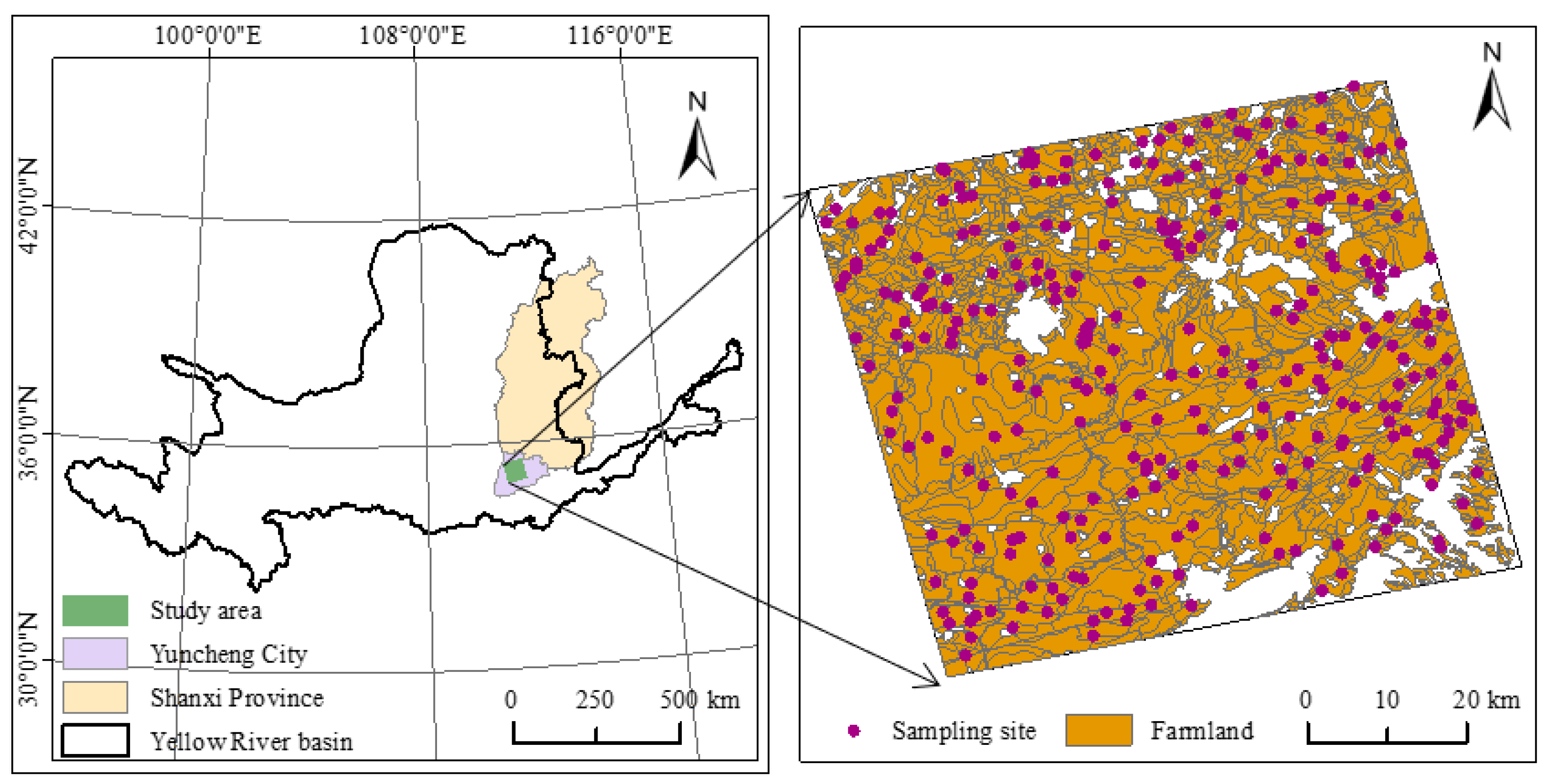
3.2. Spectral Characteristics

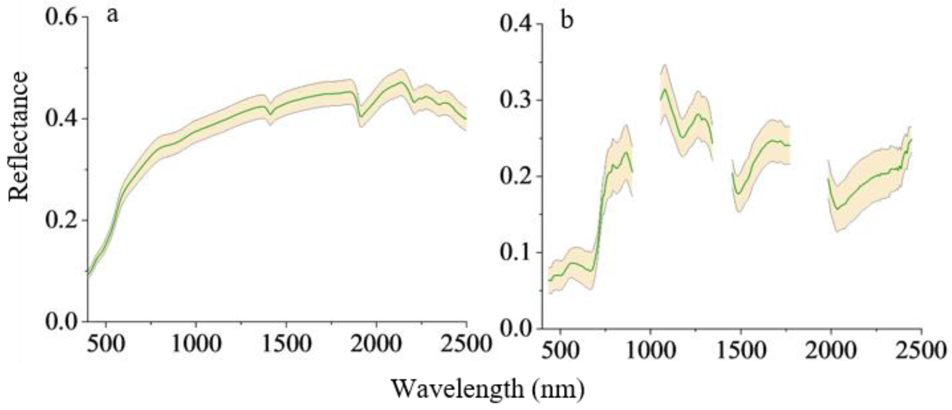
In general, the measured SOC values in the laboratory and GF-5 satellite hyperspectral curves exhibit similar spectral shapes, but there are also some differences (Figure 5). The difference in reflectance between laboratory hyperspectral and GF-5 satellite hyperspectral is mainly due to the presence of crop residues in the soil caused by the return of crop straw. Despite the SG smoothing applied to the satellite hyperspectral reflectance curves in this study, the laboratory spectral curves remained smoother than the satellite hyperspectral curves, with a smaller standard deviation. This suggests that the satellite hyperspectral data were influenced by varying degrees of noise interference. For both laboratory and satellite hyperspectral data, reflectance increased rapidly with wavelength in the 400–1000 nm range, attributed to the presence of iron ions and organic matter. However, certain differences in reflectance at various wavelengths, particularly after 2000 nm, indicated spectral distinctions under different measurement conditions, potentially affecting the accuracy of SOC prediction. The difference in reflectance between laboratory hyperspectral and GF-5 satellite hyperspectral is mainly due to the presence of crop residues in the soil caused by the return of crop straw.

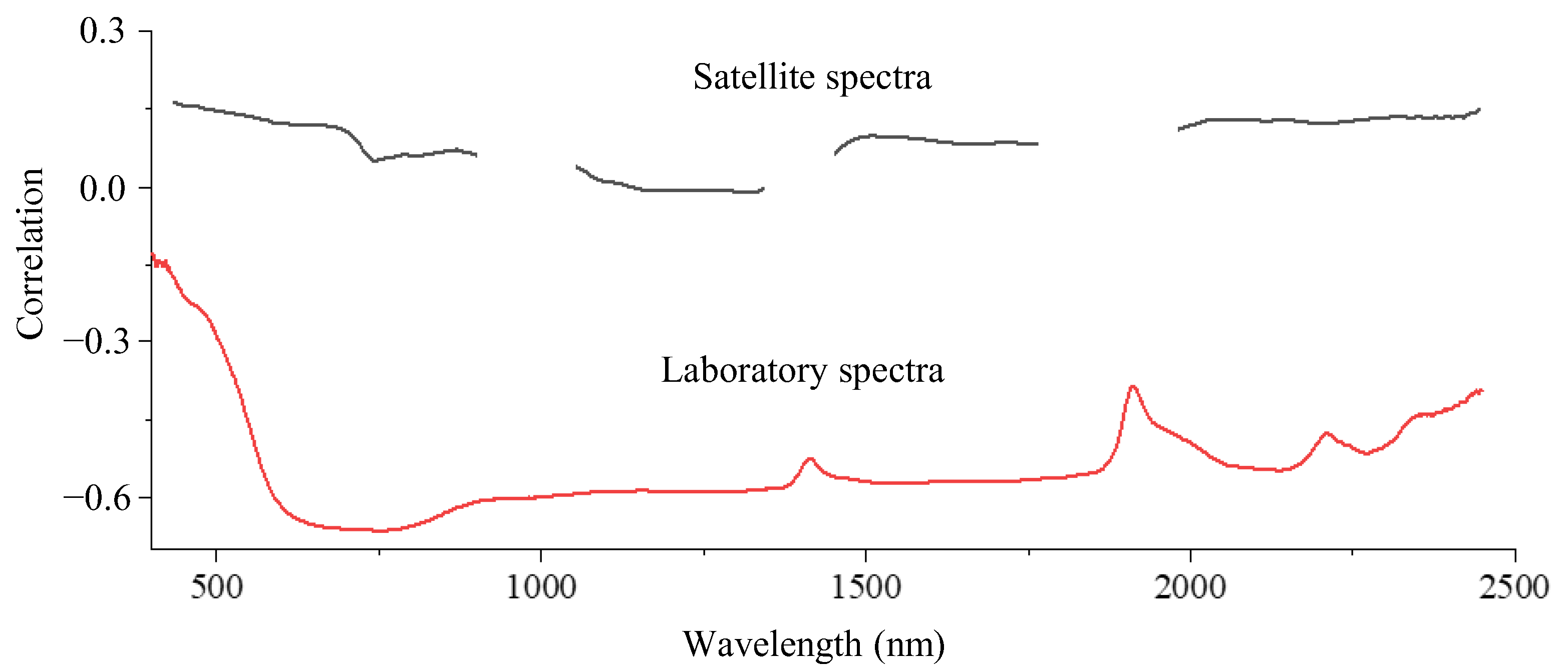
To analyze the relationship between laboratory and satellite hyperspectral spectra with SOC, the study conducted a Pearson correlation analysis between the measured SOC values and every band of laboratory and GF-5 satellite hyperspectral data (Figure 6). Results indicated that the absolute values of the correlation coefficients between measured SOC values and laboratory spectra (0.11–0.67) were much higher than those of satellite hyperspectral data (0–0.19), suggesting that the external environmental interference experienced by GF-5 satellite hyperspectral data significantly masked the relationship between SOC content and the spectral reflectance itself. Compared to laboratory hyperspectral data, satellite hyperspectral data without denoising may struggle to predict SOC content accurately.

3.3. FOD Processing of Laboratory Hyperspectral Data

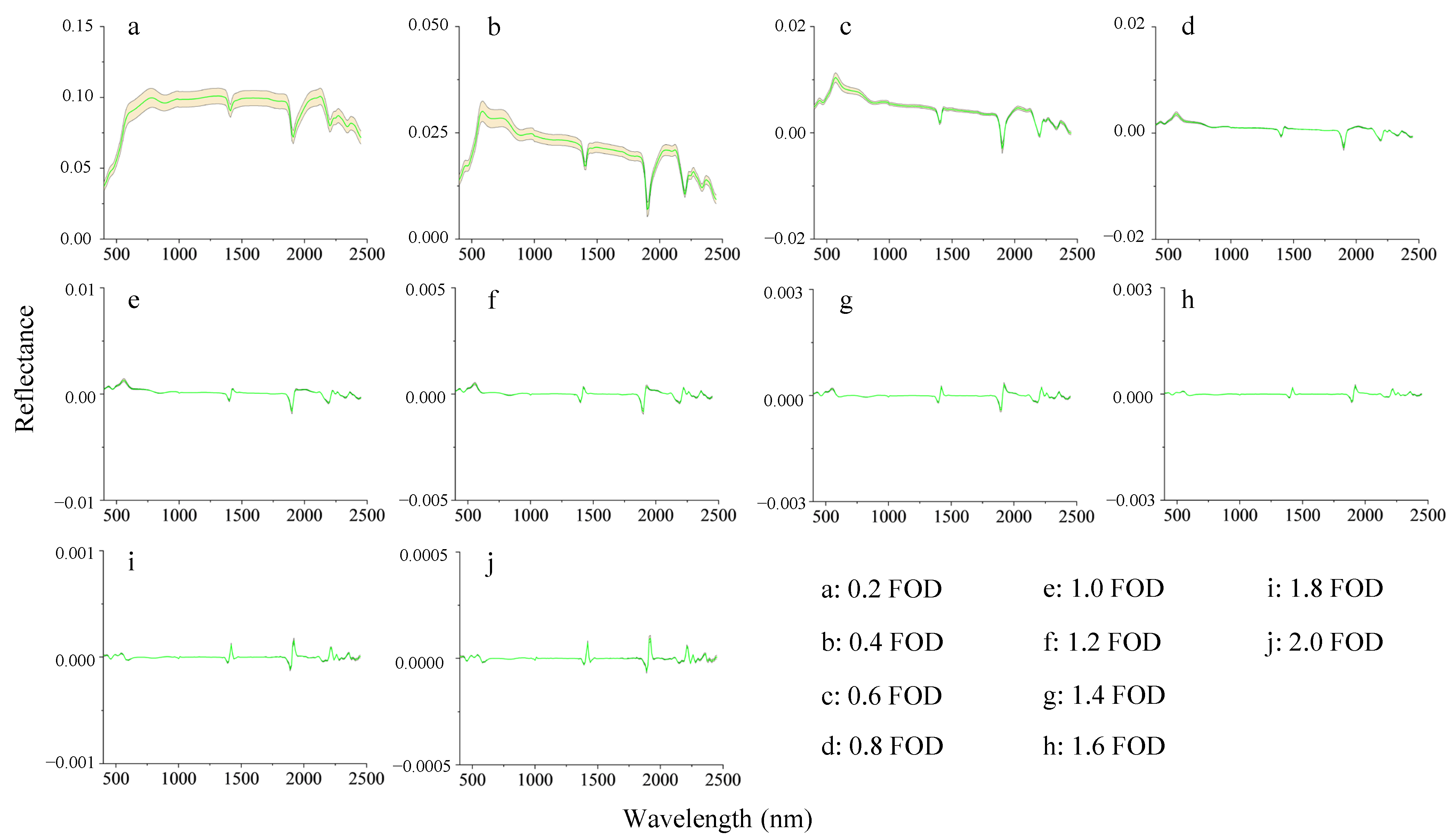
Soil hyperspectral data exhibit comprehensive spectral characteristics reflecting various soil physicochemical components, and absorption peaks of these components may interfere with each other to varying extents. Spectral derivative technology not only separates absorption peaks but also amplifies weak absorption peaks. As depicted in Figure 7, a comparison of 0–2.0 order (with intervals of 0.2 order, totaling 10 orders) derivative transformations revealed that the spectral reflectance values of laboratory spectra gradually decreased from 0 order to 0.6 order, with absorption bands narrowing and no significant distortion of absorption peaks (Figure 7a–c). In the 0.8–2.0 order derivatives, spectral reflectance curves gradually stabilized, reflectance values continued to decrease, and absorption bands continued to narrow, with the original shape of the spectrum gradually disappearing (Figure 7d–j). Although correlating spectral absorption peaks with specific components in the soil is a challenging task, FOD processing aids in extracting sensitive information.

To select the optimal order of fractional derivative for predicting SOC with laboratory hyperspectral data, this study constructed SOC prediction models using the RF model with both the original and various FOD processed spectral reflectance as independent variables, evaluating their capability in predicting SOC. The accuracy evaluation results are shown in

Table 3. Accuracy of SOC prediction models for laboratory hyperspectral data after different FOD processing.

Order	R2	RMSE	MAE
0	0.49	1.73	0.71
0.2	0.56	1.66	0.69
0.4	0.73	1.48	0.62
0.6	0.84	1.28	0.48
0.8	0.82	1.33	0.49
1.0	0.61	1.59	0.67
1.2	0.54	1.71	0.69
1.4	0.75	1.46	0.56
1.6	0.81	1.35	0.49
1.8	0.74	1.46	0.58
2.0	0.75	1.44	0.55

Note: Order 0 represents the original laboratory spectrum.

. The results indicated that models processed with FODs had stronger predictive abilities than the original spectra. Under different FODs, the inversion accuracy of SOC (R²) ranged between 0.49–0.84, with RMSE decreasing from 1.73 to 1.28, and MAE values from 0.71 to 0.48. Compared to the original hyperspectral model, the predictive abilities of the models after 0.6, 0.8, and 1.6 order derivative processing were the strongest, with the 0.6 order derivative processed model having the highest accuracy (R² = 0.84, RMSE = 1.28, MAE = 0.48). Therefore, the 0.6 order derivative is the optimal order for processing laboratory hyperspectral data.

3.4. Image Denoising of GF-5

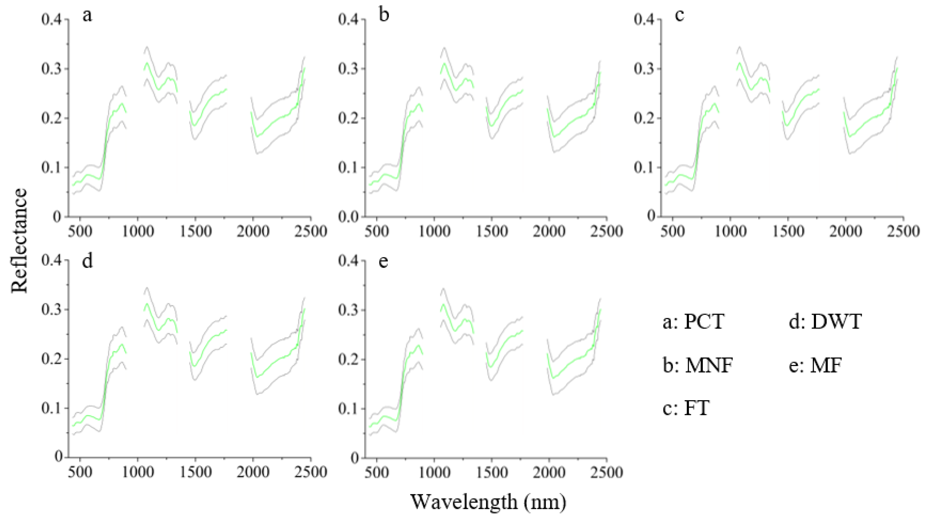
To reduce noise in satellite hyperspectral imagery, various denoising methods were applied to GF-5 hyperspectral images. Figure 8 and Figure 9 show satellite images and hyperspectral reflectance curves of GF-5 images after different denoising processes, respectively. After various denoising treatments, slight differences in color, brightness, and texture were observed in different features of the satellite images. Compared to the original satellite hyperspectral image, the denoised spectral curves were smoother, indicating that denoising could eliminate some noise from the satellite images. However, it was difficult to visually determine the best denoising method among the different approaches.

Therefore, using the hyperspectral reflectance after different denoising treatments as the independent variable and SOC as the dependent variable, SOC prediction models were constructed using the RF method to determine the optimal denoising method (

Table 4. Accuracy of SOC prediction models for GF-5 satellite hyperspectral data after various denoising treatments.

Image Denoising Method	R2	RMSE	MAE
R	0.31	2.04	0.98
PCT	0.29	2.04	1.03
MNF	0.33	1.95	0.97
FT	0.42	1.88	0.78
DWT	0.48	1.78	0.71
MF	0.22	2.12	1.19

Note: R represents the original spectrum of satellite imagery.

). The results showed that the SOC prediction accuracy decreased after median filtering compared to the original GF-5 image (Table 4), likely due to the averaging method of pixel spectral denoising in MF. Similarly, after PCT of GF-5 images, the accuracy of SOC prediction also decreased (Table 4), possibly related to the mechanism of PCT. PCT outputs new principal component bands from hyperspectral image bands (equal to the number of input spectral bands), with the first principal component containing the largest percentage of data variance, followed by the second, and so on. The last principal component bands, containing very small variances (mostly from original spectral noise), also include some image information. Moreover, GF-5 satellite hyperspectral images after MNF showed slightly stronger SOC prediction ability than the original image (Table 4). Notably, DWT and FT significantly enhanced the ability of GF-5 satellite hyperspectral images to predict SOC (Table 4). The best satellite image denoising method in this study was wavelet transformation, which, after application, showed the highest increase in SOC prediction accuracy (R² = 0.48, RMSE = 1.78, MAE = 0.71).

3.5. Optimal FOD Processing for Various Denoised Images

As demonstrated previously (Section 3.3), FODs applied to laboratory hyperspectral data significantly enhance the accuracy of SOC prediction. In order to improve the predictive capacity of satellite hyperspectral data for SOC, this study identified the FOD order that yielded the highest prediction accuracy for SOC (

Table 5. Accuracy of SOC prediction models for satellite hyperspectral data after various FOD processing.

Order	R2	RMSE	MAE
0	0.31	2.04	0.98
0.2	0.37	1.96	0.92
0.4	0.43	1.84	0.87
0.6	0.46	1.79	0.81
0.8	0.52	1.68	0.76
1.0	0.32	2.01	0.98
1.2	0.34	1.99	0.94
1.4	0.44	1.84	0.85
1.6	0.47	1.77	0.79
1.8	0.41	1.87	0.88
2.0	0.39	1.92	0.55

Note: Order 0 represents the original spectrum of satellite imagery.

) and applied it to process GF-5 images. The results indicated that after subjecting GF-5 satellite hyperspectral images to different FOD treatments, the SOC prediction accuracy (R²) increased from 0.31 to 0.52, RMSE decreased from 2.04 to 1.68, and MAE values decreased from 0.98 to 0.76. In comparison to the original hyperspectral model, the model processed with the 0.8 order derivative exhibited the most substantial improvement in predictive ability (R² = 0.52, RMSE = 1.68, MAE = 0.76). Therefore, the optimal order for processing satellite hyperspectral data is 0.8, which differs from the optimal order for processing laboratory hyperspectral data. This discrepancy could be attributed to variations in noise characteristics between laboratory and satellite hyperspectral data. It is noteworthy that, for both laboratory and satellite hyperspectral data, FOD processing demonstrated a more pronounced impact than integer order derivative processing, highlighting the superior ability of FODs to capture subtle changes in the spectrum.

Since the 0.8 order derivative processing proved to be the optimal method for predicting SOC in GF-5 satellite hyperspectral imagery, the study further denoised the 0.8 order derivative processed GF-5 satellite images and explored SOC prediction modeling using the RF model.

Table 6. Accuracy of SOC prediction models for GF-5 satellite hyperspectral data after 0.8 FOD processing with different denoising methods.

Image Denoising Method	R2	RMSE	MAE
0.8FOD-R	0.52	1.68	0.76
0.8FOD-PCT	0.47	2.04	1.03
0.8FOD-MNF	0.52	1.95	0.97
0.8FOD-FT	0.58	1.88	0.78
0.8FOD-DWT	0.61	1.78	0.71
0.8FOD-MF	0.39	2.12	1.19

Note: R represents the original GF-5 image without image denoising.

presents the modeling results, indicating that after PCT and median filtering denoising of the 0.8 order derivative processed images, the model accuracy was still lower than that of 0.8FOD-R, while 0.8FOD-MNF exhibited similar accuracy (R² = 0.52). The SOC prediction accuracy of 0.8FOD-DWT and 0.8FOD-FT significantly increased, with 0.8FOD-DWT achieving the highest accuracy (R² = 0.61, RMSE = 1.78, MAE = 0.71). Figure 10 depicts a satellite image of a local area of the GF-5 imagery after optimal noise reduction processing (0.8FOD-DWT) and its spectral reflectance chart. The 0.8FOD-DWT amplifies parts of the spectral curve, making the curve changes clearer and facilitating the distinction of differences in SOC content.

3.6. Spectral Feature Selection

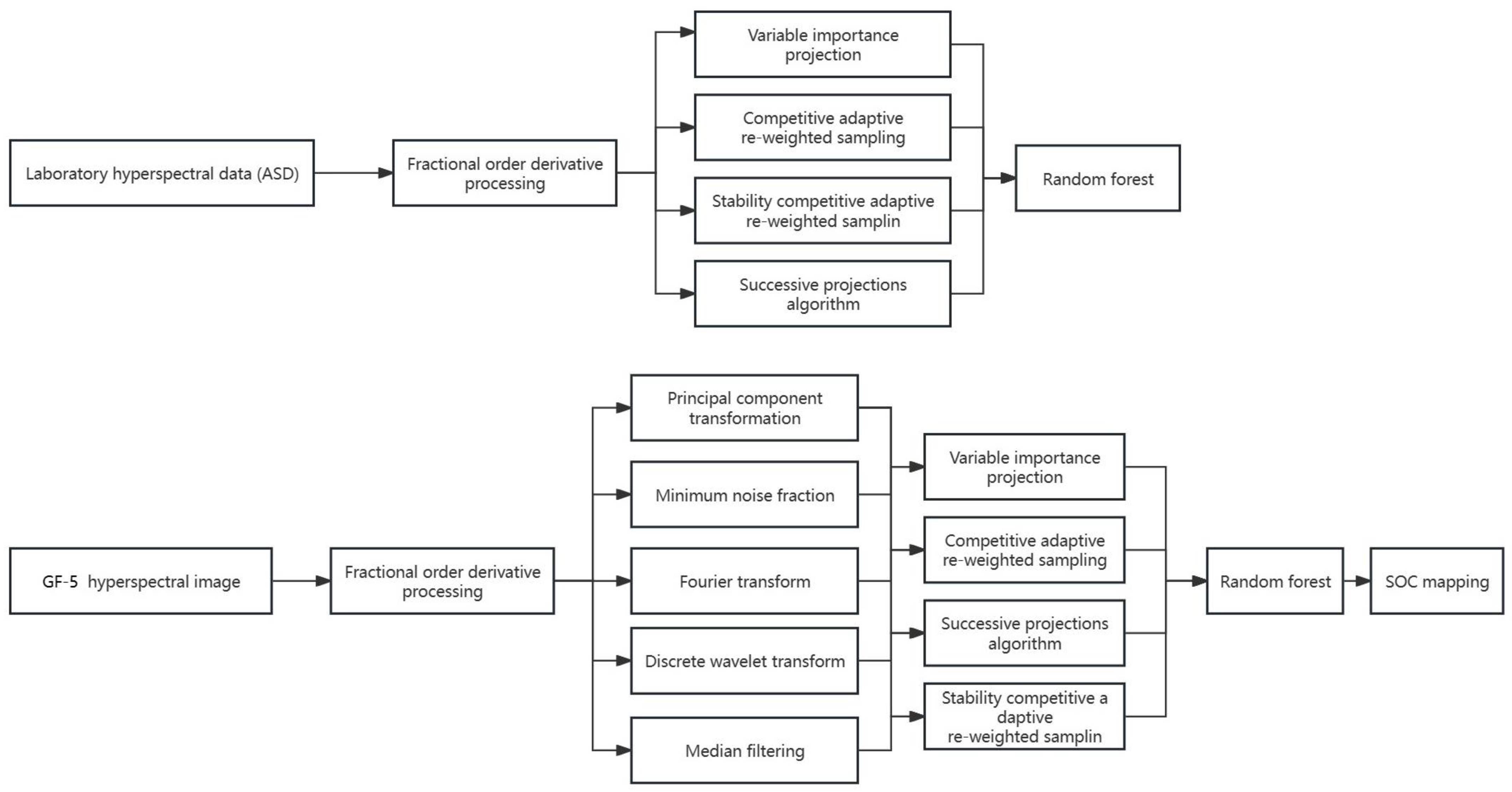
As previously mentioned, with the full bandwidth as the dependent variable for SOC modeling, the 0.6FOD was the best model for laboratory hyperspectral SOC prediction, and 0.8FOD-DWT denoised GF-5 imagery was the best for satellite hyperspectral SOC prediction. Indeed, hyperspectral data have some bands unrelated to SOC, with high overlap or collinearity between bands. Through spectral band variable extraction techniques, spectral data dimensionality can be reduced, enhancing the robustness and accuracy of the SOC hyperspectral inversion model. This study used four methods, VIP, CARS, sCARS, and SPA, to select spectral wavelength variables with the strongest explanatory power for SOC.

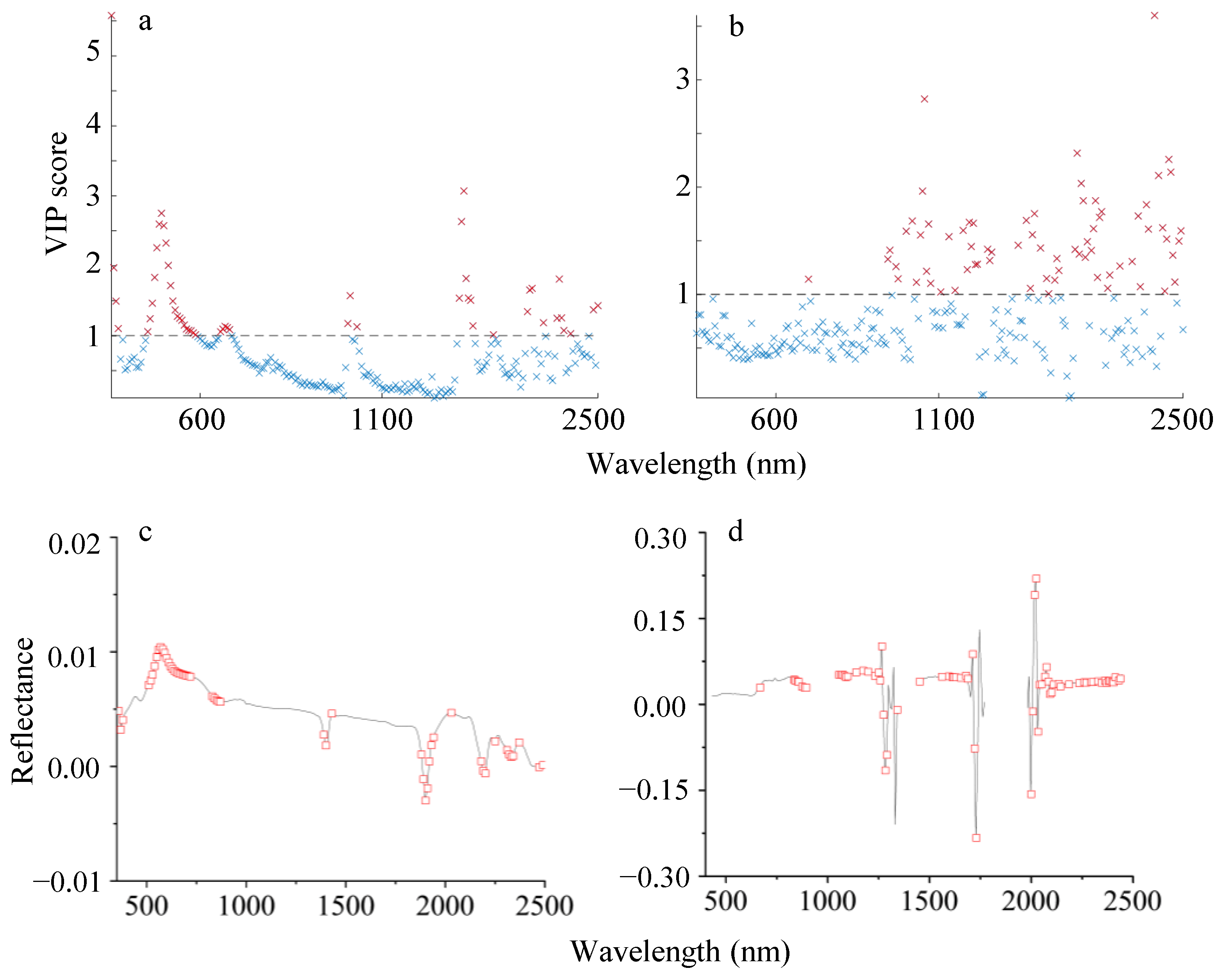
Figure 11 shows the feature band results selected by the VIP method for 0.6FOD processed laboratory hyperspectral and 0.8FOD-DWT denoised GF-5 satellite hyperspectral data. The higher the VIP score, the more significant the feature importance of the related band. To determine the optimal number of feature bands, the study set a threshold of 1.0 (Figure 11a,b). When VIP > 1.0 (above the blue dotted line), SOC feature bands of laboratory spectra were mainly located near 500 nm and in some bands between 1800–2450 nm, with the red box in Figure 11c indicating the selected feature bands, totaling 53, approximately 24.65% of the full bandwidth (Figure 11c). In contrast, SOC feature bands of satellite hyperspectral data were mainly after 1100 nm, totaling 70, approximately 29.17% of the full bandwidth (Figure 11d).

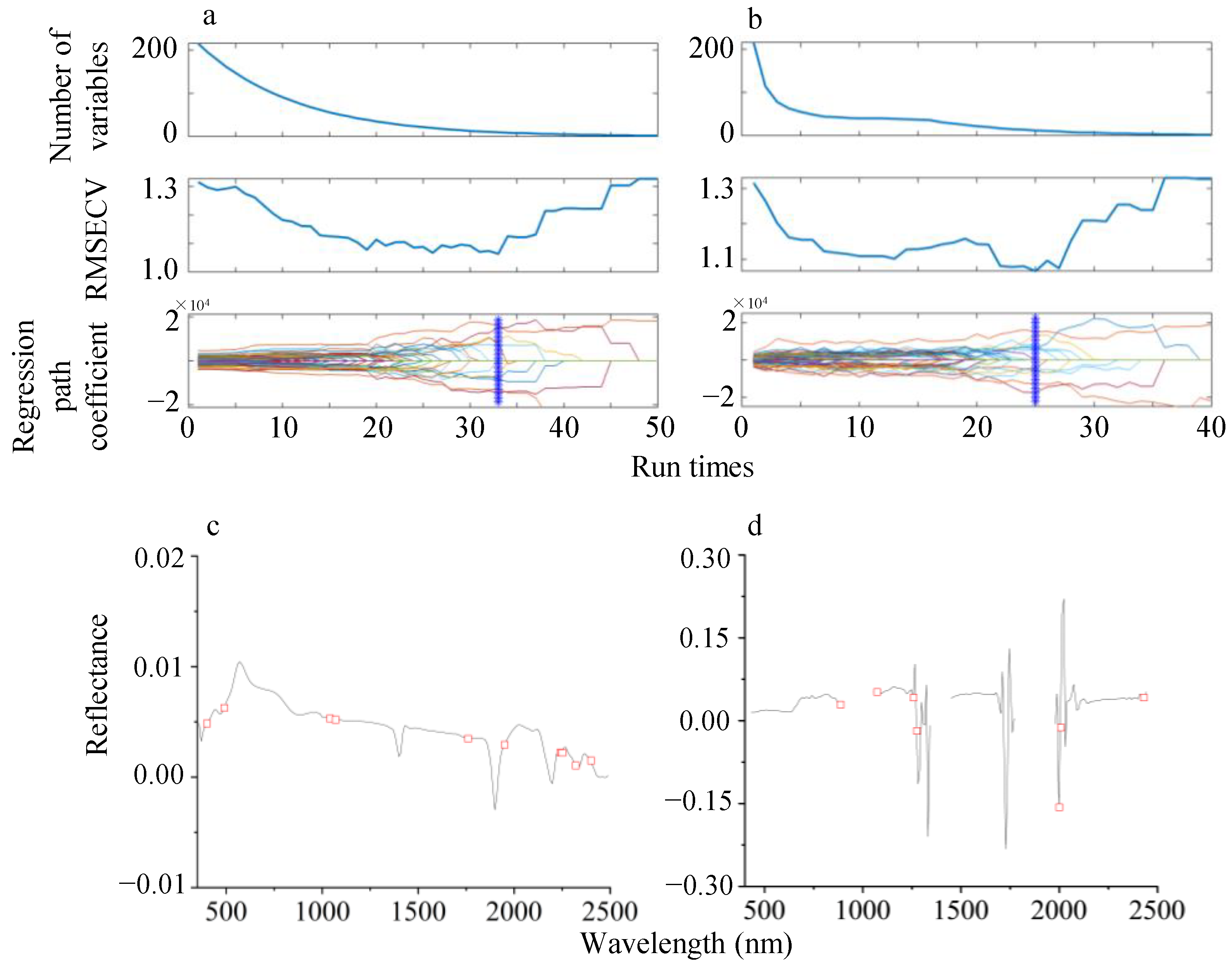
The CARS algorithm was employed to select feature bands from 0.6FOD laboratory hyperspectral data and 0.8FOD-DWT denoised GF-5 satellite hyperspectral data, as illustrated in Figure 12. The results demonstrated a gradual decrease in the number of retained wavelength variables as the number of iterations increased. The RMSECV initially decreased and then increased with the rising number of iterations (Figure 12a,b). For the 0.6FOD laboratory hyperspectral data, the minimum RMSECV value was obtained at the 17th iteration, and beyond this point, bands related to SOC may have been excluded, resulting in an increase in RMSECV value. At this stage, the optimal bands for predicting SOC were 18, accounting for approximately 8.37% of the total bands (Figure 12c). For the 0.8FOD-DWT satellite hyperspectral data, the minimum RMSECV value was observed at the 22nd iteration, with the best SOC prediction bands being 8, representing about 3.33% of the total bands (Figure 12b,d). Similarly, the sCARS algorithm was also applied (Figure 13), showing that the minimum RMSECV values for the 0.6 FOD laboratory hyperspectral data and the 0.8FOD-DWT satellite hyperspectral data were achieved at the 33rd and 25th iterations, respectively. At these points, eight and seven bands were selected as the optimal number of bands for SOC prediction, for the laboratory and satellite data, respectively (Figure 13c,d). It is noteworthy that the number of bands selected by sCARS was fewer, likely due to the algorithm’s emphasis on the stability of variables.

After processing the laboratory and GF-5 satellite hyperspectral data with 0.6FOD and 0.8FOD-DWT, respectively, the SPA algorithm was employed to extract feature bands. The determination of the number of feature bands was based on calculating the minimum RMSE values for different band combinations. The SPA algorithm results, as shown in Figure 14, indicate a significant decrease in RMSE for both laboratory and satellite hyperspectral data when the number of feature bands ranges from 1 to 21 and 1 to 5, respectively. After that, the trend gradually levels off. Specifically, for the 0.6FOD laboratory spectrum, 15 feature bands were selected (indicated by the black box in Figure 14c). Although the RMSE was smallest at 21 bands, the relationship between these bands and the measured SOC was not significant. In contrast, at 15 bands, the relationship was significant. These 15 bands represent about 6.98% of the total bands. For the satellite hyperspectral data, five feature bands were selected, accounting for approximately 2.08% of the total bands (Figure 14d).

3.7. SOC Prediction

In this study, feature bands selected using the VIP, CARS, sCARS, and SPA algorithms were employed as independent variables, with SOC as the dependent variable, to construct eight RF models. These include 0.6FOD-VIP, 0.6FOD-CARS, 0.6FOD-sCARS, and 0.6FOD-SPA based on laboratory hyperspectral data, and 0.8FOD-DWT-VIP, 0.8FOD-DWT-CARS, 0.8FOD-DWT-sCARS, and 0.8FOD-DWT-SPA based on GF-5 satellite hyperspectral data. These models were compared with full-bandwidth RF models. As per the results in

Table 7. Accuracy of SOC prediction models.

ASD	R2	RMSE	MAE	GF-5	R2	RMSE	MAE
0.6FOD-R	0.84	1.28	0.48	0.8FOD-DWT-R	0.61	1.78	0.71
0.6FOD-VIP	0.86	1.22	0.45	0.8FOD-DWT-VIP	0.62	1.77	0.71
0.6FOD-CARS	0.88	1.18	0.44	0.8FOD-DWT-CARS	0.66	1.67	0.70
0.6FOD-sCARS	0.91	1.13	0.41	0.8FOD-DWT-sCARS	0.69	1.58	0.64
0.6FOD-SPA	0.84	1.26	0.47	0.8FOD-DWT-SPA	0.58	1.81	0.74

Note: R indicates the original hyperspectral data (full bandwidth).

, the accuracy of the models with feature band selection was found to be higher than those using full-bandwidth models for both laboratory and satellite hyperspectral data. The ranking of feature band selection techniques in terms of effectiveness was sCARS > CARS > SPA > VIP. Notably, feature band selection techniques effectively eliminate redundant variables in hyperspectral bands, reduce collinearity between adjacent bands, and extract important feature information variables related to SOC. This reduction in the number of variables involved in modeling decreases the complexity of the models while maximizing their prediction accuracy. Furthermore, the feature bands selected by the sCARS algorithm performed better in predicting SOC. The R² values of 0.6 FOD-sCARS for laboratory hyperspectral and 0.8 FOD-DWT-sCARS for satellite hyperspectral models were significantly higher than those of the full-bandwidth models, with noticeably lower RMSE and MAE.

3.8. SOC Mapping and Uncertainty Analysis

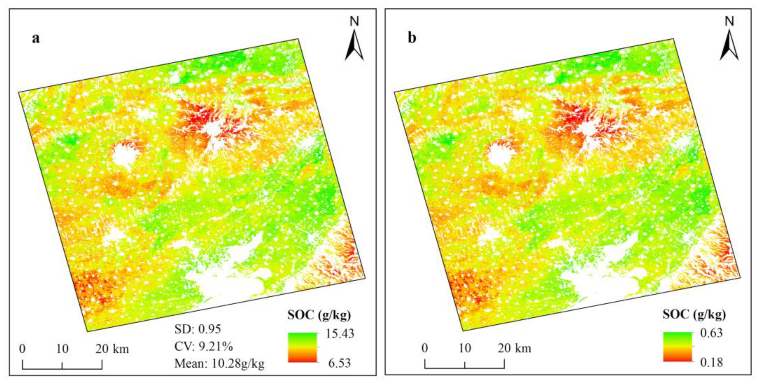
Using the RF model established with feature bands selected by the 0.8FOD-DWT-sCARS algorithm for satellite hyperspectral data, the spatial distribution of surface SOC in the study area and its associated prediction uncertainty were mapped (Figure 15). The predicted SOC values closely aligned with the actual measurements, averaging around 10.28 g/kg. The range, CV, and standard deviation of the predicted values were notably lower than those of the measured values (Figure 15a). These findings align with previous studies on SOC prediction [36], indicating a relatively stable model in terms of simulation accuracy and its ability to capture spatial heterogeneity.

The SOC spatial distribution map reveals that areas with low SOC are primarily located in high-altitude mountains, characterized by sloped, fragmented cultivated land of relatively low quality, resulting in poorer soil. Additionally, SOC generally exhibits a higher concentration in the east and lower levels in the west, potentially due to the western part’s proximity to the Yellow River, leading to relatively sandy soil. Furthermore, the results indicate that the spatial uncertainty of SOC prediction mirrors the distribution of SOC, with areas exhibiting higher SOC uncertainty also demonstrating higher content. Overall, the standard deviation of the SOC map is relatively small, ranging between 0.18–0.68 g/kg, indicating the model’s robust performance in predicting SOC.

4. Discussion

4.1. Comparison of SOC Prediction Accuracy between Laboratory and Satellite Hyperspectral Data

SOC exhibits a direct spectral response within the spectral range and is among the soil properties successfully estimated through vis-NIR. In comparison to laboratory spectra, the RF model using GF-5 satellite hyperspectral data demonstrates lower predictive performance (Table 3, Table 4 and Table 5). For instance, the R² value of the full-spectrum model for laboratory spectra is higher than that of satellite spectra. Additionally, feature band selection methods, such as VIP, CARS, sCARS, and SPA, improve SOC prediction accuracy by selecting optimal wavelength combinations. In the case of laboratory hyperspectral data (Table 7), the 0.6FOD-sCARS RF model (R² = 0.91) outperforms the 0.6FOD-R RF model (full spectrum R² = 0.84), indicating that the RF model with feature band selection after 0.6 order differential of laboratory spectra can successfully estimate surface SOC.

For satellite hyperspectral data, they also provide satisfactory predictions, with R² ranging between 0.58 to 0.69 (Table 7). The accuracy of SOC prediction using satellite hyperspectral data, processed with fractional order differentiation and image denoising, is enhanced and further improved after feature band selection. Among them, the 0.8 FOD-DWT-sCARS RF model is the best for mapping surface SOC in the entire study area. However, even the best satellite hyperspectral (0.8FOD-DWT-sCARS) prediction model for SOC is less accurate than laboratory hyperspectral data. This result aligns with previous studies [7,37], attributable to different measurement conditions such as collection height, atmospheric environment, and optical angles. Additionally, laboratory soil samples are air-dried, crushed, and sieved, whereas satellite hyperspectral data directly scan the surface, where temperature, moisture, and roughness vary greatly. These cumulative factors lead to strong noise interference in satellite hyperspectral data, negatively impacting predictive performance, despite multiple denoising methods attempted in this study. We also noticed that the optimal order for processing satellite hyperspectral data is 0.8, which is different from the optimal order for processing laboratory hyperspectral data (0.6-order). It is different from previous studies, the optimal order for processing airborne hyperspectral data (0.75-order) [38], satellite hyperspectral data (0.8-order) [20], and laboratory-measured hyperspectral data (1.2-order) [39] (1.25-order) [40]. This discrepancy could be attributed to variations in noise characteristics between laboratory and satellite hyperspectral data. It is noteworthy that, for both laboratory and satellite hyperspectral data, FOD processing demonstrated a more pronounced impact than integer order derivative processing, highlighting the superior ability of FODs to capture subtle changes in the spectrum.

Moreover, laboratory hyperspectral data are not spatially continuous and cannot capture the spatial distribution of regional SOC, whereas satellite hyperspectral imagery can provide a continuous SOC spatial distribution. In our study, the best satellite hyperspectral model had an R² = 0.69, meaning about 31% of SOC variability information was not revealed, suggesting a need to combine other pedogenic factors to further enhance the simulation accuracy of satellite hyperspectral data in predicting SOC.

4.2. Advantages of Image Denoising in Satellite Hyperspectral Prediction of SOC

Image denoising plays a crucial role in reducing noise in satellite hyperspectral images, and different denoising methods yield varying effects. In this study, satellite hyperspectral images processed through median filtering, PCT, and minimum noise transformation resulted in significant loss of spatial information during the denoising process, leading to reduced accuracy in SOC prediction. MF can protect signal edges from blurring but is less effective in suppressing random noise, failing to effectively eliminate noise in the satellite hyperspectral data. This denoising method averaged the spectral reflectance in local areas, weakening the spatial differences in the spectrum, thus, adversely affecting spatial prediction of SOC. PCT reduces noise while also affecting image quality, thereby weakening the predictive ability for SOC. MNF is essentially two cascaded PCTs, where the transformed vectors are uncorrelated, and the first component concentrates much of the information. As dimensions increase, image quality gradually declines, sorted by signal-to-noise ratio, unlike PCT sorted by variance. This overcomes the noise impact on image quality, making it superior to PCT. DWT and FT exhibited superior predictive performance, as they set the optimal scale for the lowest positive wave component and layers for different images, concentrating information on reflectance changes and interference noise in the high-frequency area, and keeping information on smooth reflectance changes in the low-frequency area for reconstruction. This mechanism effectively reduces noise in the image and preserves spectral information. SOC changes are non-stationary and non-linear, and wavelet and Fourier transformations have clear advantages in processing non-stationary data [41,42]. Consistent with our research, Meng et al. also demonstrated that DWT is an effective method for reducing noise in hyperspectral images [20]. DWT decomposes data into multiple layers (scales), and as the number of decompositions increases, data dimensions decrease, making it challenging to compare wavelet coefficients across different scales [43]. In this study, inverse DWT was employed to reconstruct wavelet coefficients at different scales, producing denoised images. Compared to other methods, DWT can perform spectral analysis of local signals, effectively reducing noise in images [44], and preserving important spatial and texture information. Its performance in predicting SOC surpasses that of other denoising methods.

4.3. Feature Band Selection

Optimal band selection stands as a powerful mathematical tool that fully considers the strong interactions between hyperspectral bands, minimizing collinearity among bands. Previous studies have demonstrated that feature band selection enhances the relationship between SOC and spectral features, thereby improving the prediction accuracy of SOC. Our study further revealed that feature bands obtained through feature band selection algorithms typically outperform full-spectrum data in predicting SOC. For both laboratory and satellite hyperspectral data, the sCARS algorithm outperformed VIP, CARS, and SPA algorithms (Table 7). The sCARS algorithm utilizes an advanced two-step method to eliminate redundant variables, offering high stability and great potential in identifying sensitive spectral variables related to SOC content. In our study, the sCARS algorithm’s feature bands provided the highest prediction accuracy for SOC. However, whether similar results can be achieved for other soil properties requires further study, as different soil properties vary in their sensitivity to spectral bands.

5. Conclusions

This study utilized laboratory and GF-5 satellite hyperspectral data to predict and map topsoil SOC in regional farmlands. We identified the best prediction models using fractional differential transformation, various denoising methods, feature band selection, and the RF model, and compared the effectiveness of laboratory and satellite hyperspectral data in predicting SOC. The conclusions are as follows:

• Feature band selection significantly improves SOC prediction accuracy for both laboratory and satellite hyperspectral data, with sCARS being the most effective in enhancing the accuracy of SOC prediction models.
• The 0.6FOD-sCARS RF model is the best combination for predicting SOC with laboratory hyperspectral data (R² = 0.91), and the 0.8FOD-DWT-sCARS RF model is the best for satellite hyperspectral data (R² = 0.69). Satellite hyperspectral data can complement the spatial limitations of laboratory hyperspectral data, allowing for the prediction and mapping of regional SOC spatial distribution.

References

1. McBratney, A.B.; Stockmann, U.; Angers, D.A.; Minasny, B.; Field, D.J. Challenges for soil organic carbon research. In Soil Carbon; Springer International: Cham, Switzerland, 2014; pp. 3–16. [Google Scholar]
2. Chen, S.; Arrouays, D.; Angers, D.A.; Martin, M.P.; Walter, C. Soil carbon stocks under different land uses and the applicability of the soil carbon saturation concept. Soil. Tillage Res. 2019, 188, 53–58. [Google Scholar] [CrossRef]
3. Minasny, B.; Malone, B.P.; McBratney, A.B.; Angers, D.A.; Arrouays, D.; Chambers, A.; Chaplot, V.; Chen, Z.-S.; Cheng, K.; Das, B.S.; et al. Soil carbon 4 per mille. Geoderma 2017, 292, 59–86. [Google Scholar] [CrossRef]
4. Pouladi, N.; Møller, A.B.; Tabatabai, S.; Greve, M.H. Mapping soil organic matter contents at field level with Cubist, Random Forest and kriging. Geoderma 2019, 342, 85–92. [Google Scholar] [CrossRef]
5. McBratney, A.; de Gruijter, J.; Bryce, A. Pedometrics timeline. Geoderma 2019, 338, 568–575. [Google Scholar] [CrossRef]
6. McBratney, A.B.; Santos, M.L.M.; Minasny, B. On digital soil mapping. Geoderma 2003, 117, 3–52. [Google Scholar] [CrossRef]
7. Hong, Y.; Chen, S.; Chen, Y.; Linderman, M.; Mouazen, A.M.; Liu, Y.; Guo, L.; Yu, L.; Liu, Y.; Cheng, H.; et al. Comparing laboratory and airborne hyperspectral data for the estimation and mapping of topsoil organic carbon: Feature selection coupled with Random Forest. Soil. Tillage Res. 2020, 199, 104589. [Google Scholar] [CrossRef]
8. Tian, H.; Zhang, J.; Zheng, Y.; Shi, J.; Qin, J.; Ren, X.; Bi, R. Prediction of soil organic carbon in mining areas. Catena 2022, 215, 106311. [Google Scholar] [CrossRef]
9. Mendes, W.S.; Sommer, M. Advancing soil organic carbon and total nitrogen modelling in peatlands: The impact of environmental variable resolution and vis-NIR spectroscopy integration. Agronomy 2023, 13, 1800. [Google Scholar] [CrossRef]
10. Cao, Y.; Bao, N.; Liu, S.; Zhao, W.; Li, S. Reducing moisture effects on soil organic carbon content prediction in visible and near-infrared spectra with an external parameter othogonalization algorithm. Can. J. Soil. Sci. 2020, 100, 253–262. [Google Scholar] [CrossRef]
11. Kovács, Z.A.; Mészáros, J.; Árvai, M.; Laborczi, A.; Szatmári, G.; László, P.; Pásztor, L. Testing PRISMA hyperspectral satellite imagery in predicting soil carbon content based on synthetized LUCAS spectral data. In Proceedings of the Copernicus Meetings, Online, 19–30 April 2021. [Google Scholar]
12. Ward, K.J.; Chabrillat, S.; Brell, M.; Castaldi, F.; Spengler, D.; Foerster, S. Mapping soil organic carbon for airborne and simulated EnMAP imagery using the LUCAS soil database and a local PLSR. Remote Sens. 2020, 12, 3451. [Google Scholar] [CrossRef]
13. Kharintsev, S.S.; Salakhov, M.K. A simple method to extract spectral parameters using fractional derivative spectrometry. Spectrochim. Acta A 2004, 60, 2125–2133. [Google Scholar] [CrossRef]
14. Mzid, N.; Pignatti, S.; Pascucci, S.; Huang, W.; Casa, R. Development of a tool for automatic bare soil detection from multitemporal satellite optical imagery for digital soil mapping applications. In IOP Conference Series: Earth and Environmental Science; IOP Publishing: Bristol, UK, 2020; Volume 509, p. 012039. [Google Scholar]
15. Raj, A.; Chakraborty, S.; Duda, B.M.; Weindorf, D.C.; Li, B.; Roy, S.; Sarathjith, M.C.; Das, B.S.; Paulette, L. Soil mapping via diffuse reflectance spectroscopy based on variable indicators: An ordered predictor selection approach. Geoderma 2018, 314, 146–159. [Google Scholar] [CrossRef]
16. Vohland, M.; Ludwig, M.; Thiele-Bruhn, S.; Ludwig, B. Determination of soil properties with visible to near-and mid-infrared spectroscopy: Effects of spectral variable selection. Geoderma 2014, 223, 88–96. [Google Scholar] [CrossRef]
17. Nelson, D.W.; Sommers, L.E. A rapid and accurate procedure for estimation of organic carbon in soils. Proc. Indiana Acad. Sci. 1974, 84, 456–462. [Google Scholar]
18. Li, B.; Xie, W. Adaptive fractional differential approach and its application to medical image enhancement. Comput. Electr. Eng. 2015, 45, 324–335. [Google Scholar] [CrossRef]
19. Sierociuk, D.; Skovranek, T.; Macias, M.; Podlubny, I.; Petras, I.; Dzielinski, A.; Ziubinski, P. Diffusion process modeling by using fractional-order models. Appl. Math. Comput. 2015, 257, 2–11. [Google Scholar] [CrossRef]
20. Meng, X.; Bao, Y.; Ye, Q.; Liu, H.; Zhang, X.; Tang, H.; Zhang, X. Soil organic matter prediction model with satellite hyperspectral image based on optimized denoising method. Remote Sens. 2021, 13, 2273. [Google Scholar] [CrossRef]
21. Liu, H.; Bao, Y.; Meng, X.; Cui, Y.; Zhang, A.; Liu, Y.; Wang, D. Soil organic matter inversion based on Gaofen-5 imagery under different noise reduction methods. J. Agri Eng. 2020, 36, 90–98. [Google Scholar]
22. Chen, G.Y.; Xie, W.; Qian, S.E. Hyperspectral imagery denoising using minimum noise fraction and VBM3D. J. Appl. Remote Sens. 2021, 15, 32208. [Google Scholar] [CrossRef]
23. Iwen, M.A. Combinatorial sublinear-time Fourier algorithms. Found. Comput. Math. 2010, 10, 303–338. [Google Scholar] [CrossRef]
24. Yang, L.; Song, M.; Zhu, A.X.; Qin, C.; Zhou, C.; Qi, F.; Li, X.; Chen, Z.; Gao, B. Predicting soil organic carbon content in croplands using crop rotation and Fourier transform decomposed variables. Geoderma 2019, 340, 289–302. [Google Scholar] [CrossRef]
25. Chen, H. Hyperspectral Estimation Study of Soil’s Main Nutrient Content. Ph.D. Thesis, Shandong Agricultural University, Tai’an, China, 2013. [Google Scholar]
26. Bao, Y. Study on the Inversion of Cultivated Soil Organic Matter Based on Gaofen-5 Hyperspectral Remote Sensing Images. Master’s Thesis, Northeast Agricultural University, Harbin, China, 2021. [Google Scholar]
27. Malmir, M.; Tahmasbian, I.; Xu, Z.; Farrar, M.B.; Bai, S.H. Prediction of soil macro-and micro-elements in sieved and ground air-dried soils using laboratory-based hyperspectral imaging technique. Geoderma 2019, 340, 70–80. [Google Scholar] [CrossRef]
28. Li, H.; Liang, Y. New methods for variable selection in high-dimensional data. In Abstracts of the 27th Academic Annual Meeting of the Chinese Chemical Society, Session 15; Chinese Chemical Society: Beijing, China, 2010. [Google Scholar]
29. Li, G.; Gao, X.; Xiao, N.; Xiao, Y. Estimation of soil organic matter content based on sCARS-RF algorithm and hyperspectral data. J. Lumin. 2019, 40, 1030–1039. [Google Scholar]
30. Hu, Y. Estimation Study of Cultivated Soil Fertility Attributes Based on Visible-Near Infrared Hyperspectral Remote Sensing. Ph.D. Thesis, Qinghai Normal University, Xining, China, 2023. [Google Scholar]
31. Breiman, L. Random Forests. Mach. Learn. 2001, 45, 5–32. [Google Scholar] [CrossRef]
32. R Core Team. A Language and Environment for Statistical Computing; R foundation for statistical computing; R Core Team: Vienna, Austria, 2016. [Google Scholar]
33. Ottoy, S.; Vos, B.D.; Sindayihebura, A.; Hermy, M.; Orshoven, J.V. Assessing soil organic carbon stocks under current and potential forest cover using digital soil mapping and spatial generalisation. Ecol. Indic. 2017, 77, 139–150. [Google Scholar] [CrossRef]
34. Tian, H.; Liu, S.; Zhu, W.; Zhang, J.; Zheng, Y.; Shi, J.; Bi, R. Deciphering the drivers of net primary productivity of vegetation in mining areas. Remote Sens. 2022, 14, 4177. [Google Scholar] [CrossRef]
35. He, X.; Yang, L.; Li, A.; Zhang, L.; Shen, F.; Cai, Y.; Zhou, C. Soil organic carbon prediction using phenological parameters and remote sensing variables generated from Sentinel-2 images. Catena 2021, 205, 105442. [Google Scholar] [CrossRef]
36. Adhikari, K.; Hartemink, A.E. Digital mapping of topsoil carbon content and changes in the driftless area of Wisconsin, USA. Soil. Sci. Soc. Am. J. 2015, 79, 155–164. [Google Scholar] [CrossRef]
37. Nouri, M.; Gomez, C.; Gorretta, N.; Roger, J.M. Clay content mapping from airborne hyperspectral Vis-NIR data by transferring a laboratory regression model. Geoderma 2017, 298, 54–66. [Google Scholar] [CrossRef]
38. Hong, Y.S.; Guo, L.; Chen, S.C.; Linderman, M.; Mouazem, A.M.; Yu, L.; Chen, Y.Y.; Liu, Y.L.; Liu, Y.F.; Cheng, H.; et al. Exploring the potential of airborne hyperspectral image for estimating topsoil organic carbon: Effects of fractional-order derivative and optimal band combination algorithm. Geoderma 2020, 365, 114228. [Google Scholar] [CrossRef]
39. Wang, X.P.; Zhang, F.; Kung, H.T.; Johnson, V.C. New methods for improving the remote sensing estimation of soil organic matter content (SOMC) in the Ebinur Lake Wetland National Nature Reserve (ELWNNR) in northwest China. Remote Sens. Environ. 2018, 218, 104–118. [Google Scholar] [CrossRef]
40. Hong, Y.S.; Liu, Y.L.; Chen, Y.Y.; Liu, Y.F.; Yu, L.; Liu, Y.; Cheng, H. Application of fractional-order derivative in the quantitative estimation of soil organic matter content through visible and near-infrared spectroscopy. Geoderma 2019, 337, 758–769. [Google Scholar] [CrossRef]
41. Reis, M.S.; Saraiva, P.M.; Bakshi, B.R. Denoising and Signal-to-Noise Ratio Enhancement: Wavelet Transform and Fourier Transform. Compr. Chemom. 2009, 2, 25–55. [Google Scholar]
42. Dai, X.P.; Cheng, L.Z.; Mareschal, J.C.; Lemire, D.; Liu, C. New method for denoising borehole transient electromagnetic data with discrete wavelet transform. J. Appl. Geophys. 2019, 168, 41–48. [Google Scholar] [CrossRef]
43. Blackburn, G.A.; Ferwerda, J.G. Retrieval of chlorophyll concentration from leaf reflectance spectra using wavelet analysis. Remote Sens. Environ. 2008, 112, 1614–1632. [Google Scholar] [CrossRef]
44. Biswas, A. Scale–location specific soil spatial variability: A comparison of continuous wavelet transform and Hilbert–Huang transform. CATENA 2018, 160, 24–31. [Google Scholar] [CrossRef]
Figure 1. Location and sampling points distribution in the study area.
Agronomy 14 00175 g001
Figure 2. Satellite image during the sampling period.
Agronomy 14 00175 g002
Figure 3. Measurement position scheme for ASD Field Spec4 spectrophotometer.
Agronomy 14 00175 g003
Figure 4. Laboratory and GF-5 image hyperspectral processing flowchart.
Agronomy 14 00175 g004
Figure 5. Average original spectral reflectance of soil samples. (a) Laboratory spectrum; (b) satellite spectrum. The yellow area illustrates the standard deviation of the spectrum.
Agronomy 14 00175 g005
Figure 6. Correlation coefficients between SOC content and laboratory and GF-5 hyperspectral data.
Agronomy 14 00175 g006
Figure 7. Laboratory hyperspectral curves after FOD processing. The yellow area illustrates the standard deviation of the spectrum.
Agronomy 14 00175 g007
Figure 8. Local area images of GF-5 satellite imagery under various denoising treatments.
Agronomy 14 00175 g008
Figure 9. Hyperspectral curves of GF-5 satellite images after various denoising treatments. The green line represents the average soil spectral features, while the gray lines depict the upper and lower boundaries of the spectral standard deviation.
Agronomy 14 00175 g009
Figure 10. Local area image and spectral reflectance of GF-5 satellite imagery processed with 0.8 FOD-DWT. The green line represents the average soil spectral features, and the yellow area indicates the standard deviation of the spectrum.
Agronomy 14 00175 g010
Figure 11. Feature bands selected by VIP. (a) and (b) represent the band VIP score results for laboratory hyperspectral and GF-5 satellite hyperspectral data, respectively. The blue dashed line indicates bands with VIP > 1 (marked with red "×" above the line) and bands with VIP < 1 (marked with blue "×" below the line). The bands with VIP > 1 are the selected characteristic bands, corresponding to the red-highlighted boxes in (c) and (d).
Agronomy 14 00175 g011
Figure 12. (a) and (b) represent the process of selecting the optimal number of bands through CARS for laboratory hyperspectral and GF-5 satellite hyperspectral data, respectively. The red-highlighted boxes in (c) and (d) indicate the characteristic bands selected by CARS for laboratory hyperspectral and GF-5 satellite hyperspectral data, respectively.
Agronomy 14 00175 g012
Figure 13. (a) and (b) represent the process of selecting the optimal number of bands through sCARS for laboratory hyperspectral and GF-5 satellite hyperspectral data, respectively. The red-highlighted boxes in (c) and (d) indicate the characteristic bands selected by sCARS for laboratory hyperspectral and GF-5 satellite hyperspectral data, respectively.
Agronomy 14 00175 g013
Figure 14. (a) and (b) show the optimal number of bands selected through SPA for laboratory hyperspectral and GF-5 satellite hyperspectral data, respectively. The black-highlighted boxes represent the optimal number of bands. The red-highlighted boxes indicate the characteristic bands selected by SPA for laboratory hyperspectral (c) and GF-5 satellite hyperspectral (d) data.
Agronomy 14 00175 g014
Figure 15. (a) Spatial distribution map of SOC in the study area; (b) Map of prediction uncertainty.
Agronomy 14 00175 g015