Sensitivity Analysis of the WOFOST Crop Model Parameters Using the EFAST Method and Verification of Its Adaptability in the Yellow River Irrigation Area, Northwest China

Abstract
:1. Introduction
2. Materials and Methods
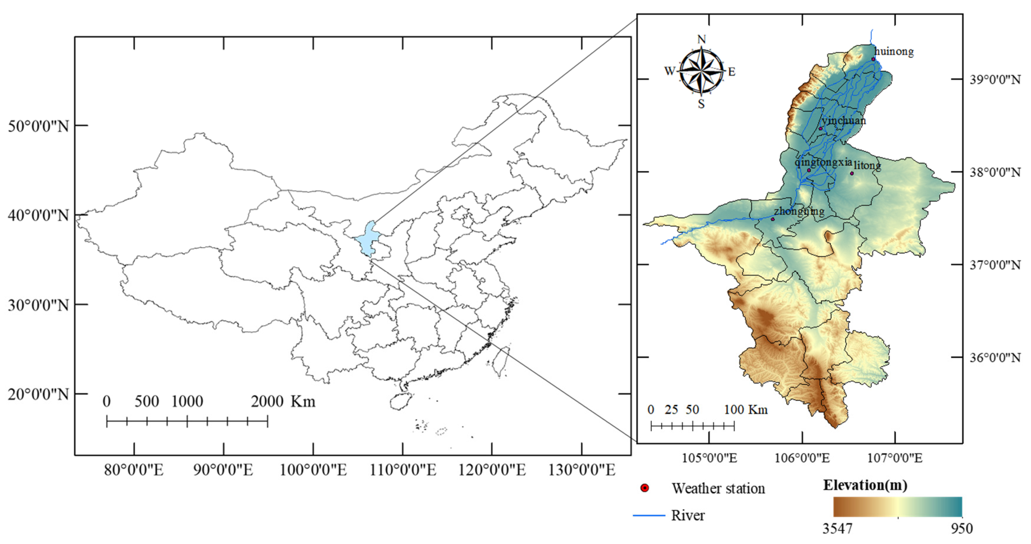
2.1. Overview and Data Sources of the Study Area
2.2. WOFOST Model
2.3. Structural Equation Model
2.4. Research Methods
2.4.1. Crop Model Parameter Selection Method in WOFOST Model
2.4.2. EFAST Analysis Method
2.4.3. Analysis Scheme
- (1)
- Python 3.7 program calculated soil and meteorological files according to the test area’s soil and meteorological conditions. The value range and distribution form of the input crop parameters were defined in SimLab 2.2.
- (2)
- The Monte Carlo method randomly sampled parameters, with 2835 sampling times taken (the EFAST method considered that the analysis results with sampling times > number of parameters × 65 were valid).
- (3)
- The generated parameter set was written into the corresponding WOFOST model file. The model was then run, and the simulation results were organized.
- (4)
- The simulated data was formatted into text for recognitionn by the SimLab 2.2, followed by conducting Monte Carlo analysis through SimLab 2.2 and obtaining the final SA result.
- (5)
- Based on the analysis results, parameters with a high sensitivity index were selected to establish SEMs, which were analyzed and visualized using the RStudio2021.09.0 program.
- (6)
- Crop parameters were adjusted according to crop parameter sensitivity and contribution analysis. The WOFOST model was run with meteorological and soil files of other sites for localization verification.
2.4.4. Model Consistency Test Method
3. Results and Analysis
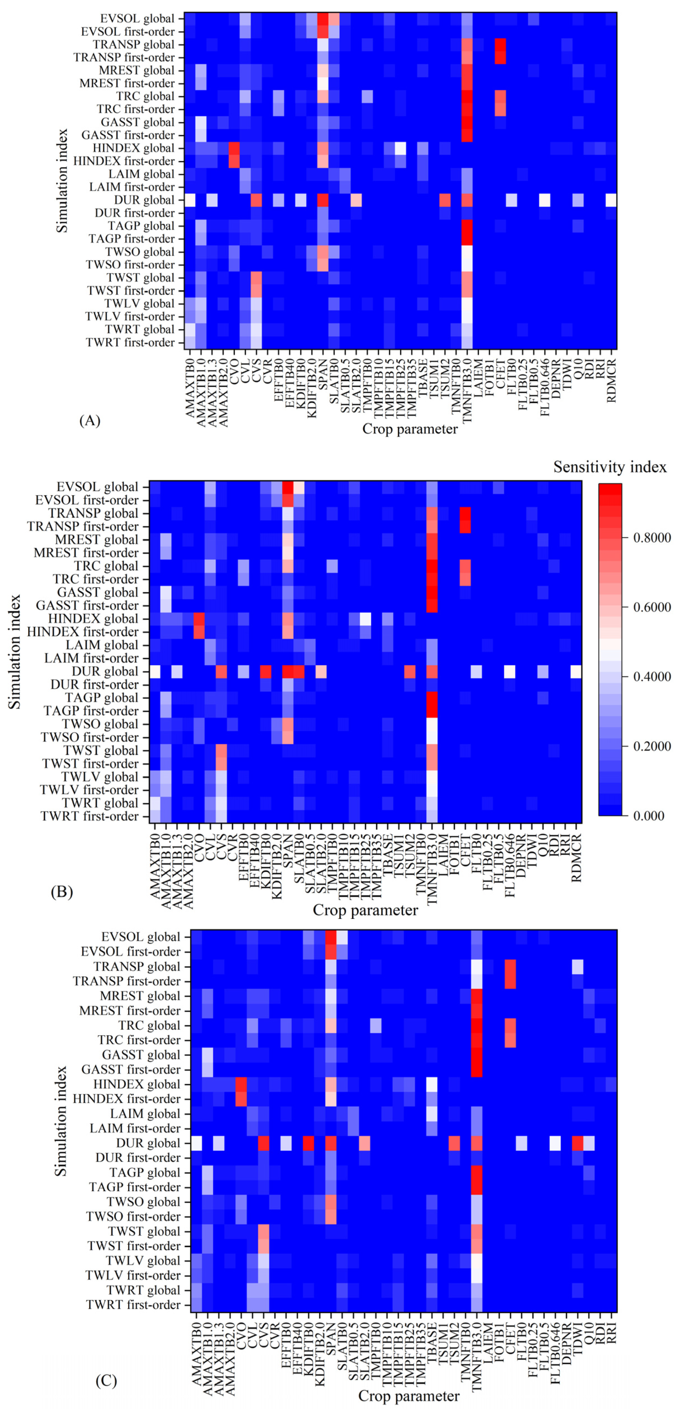
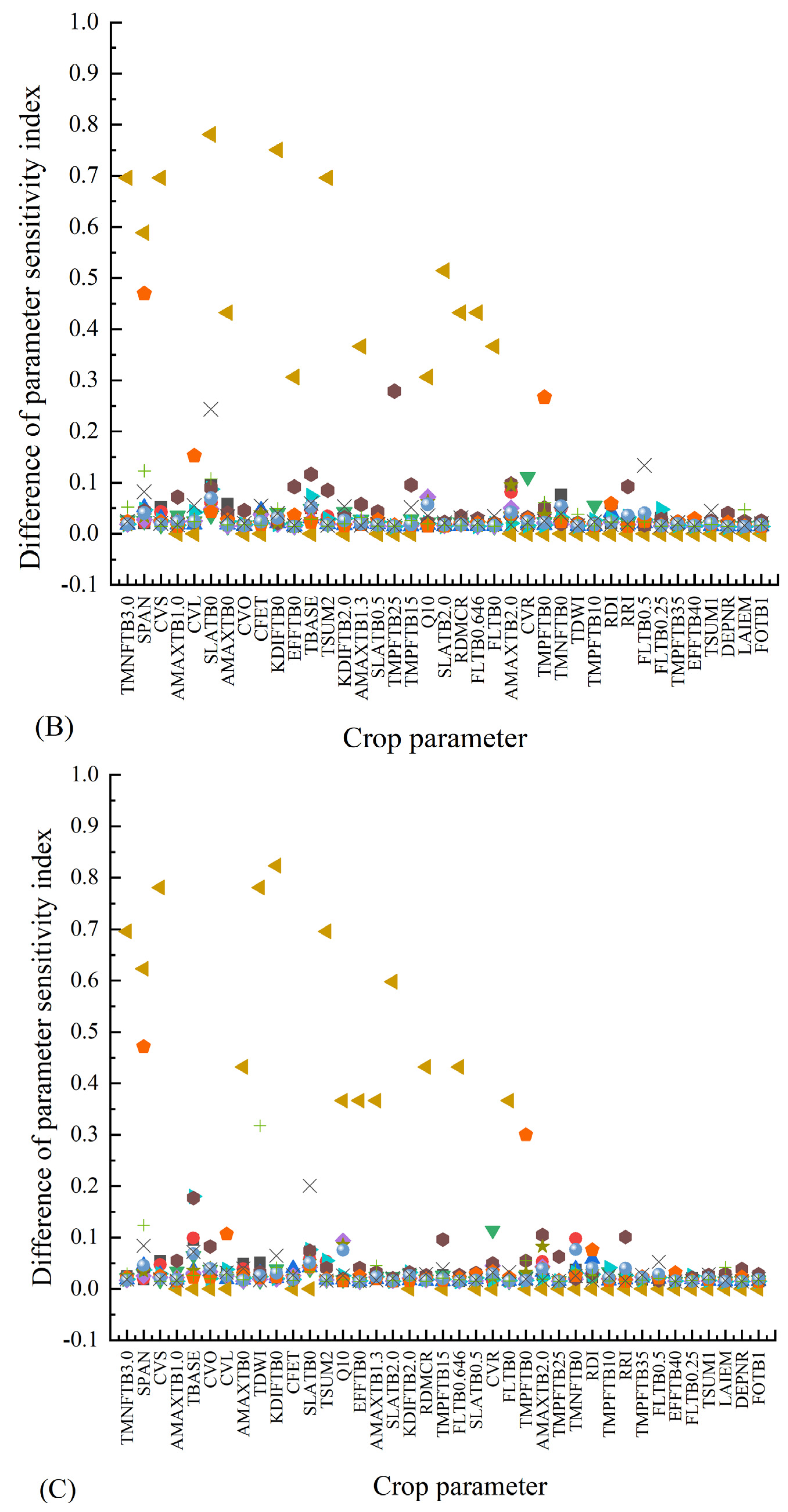
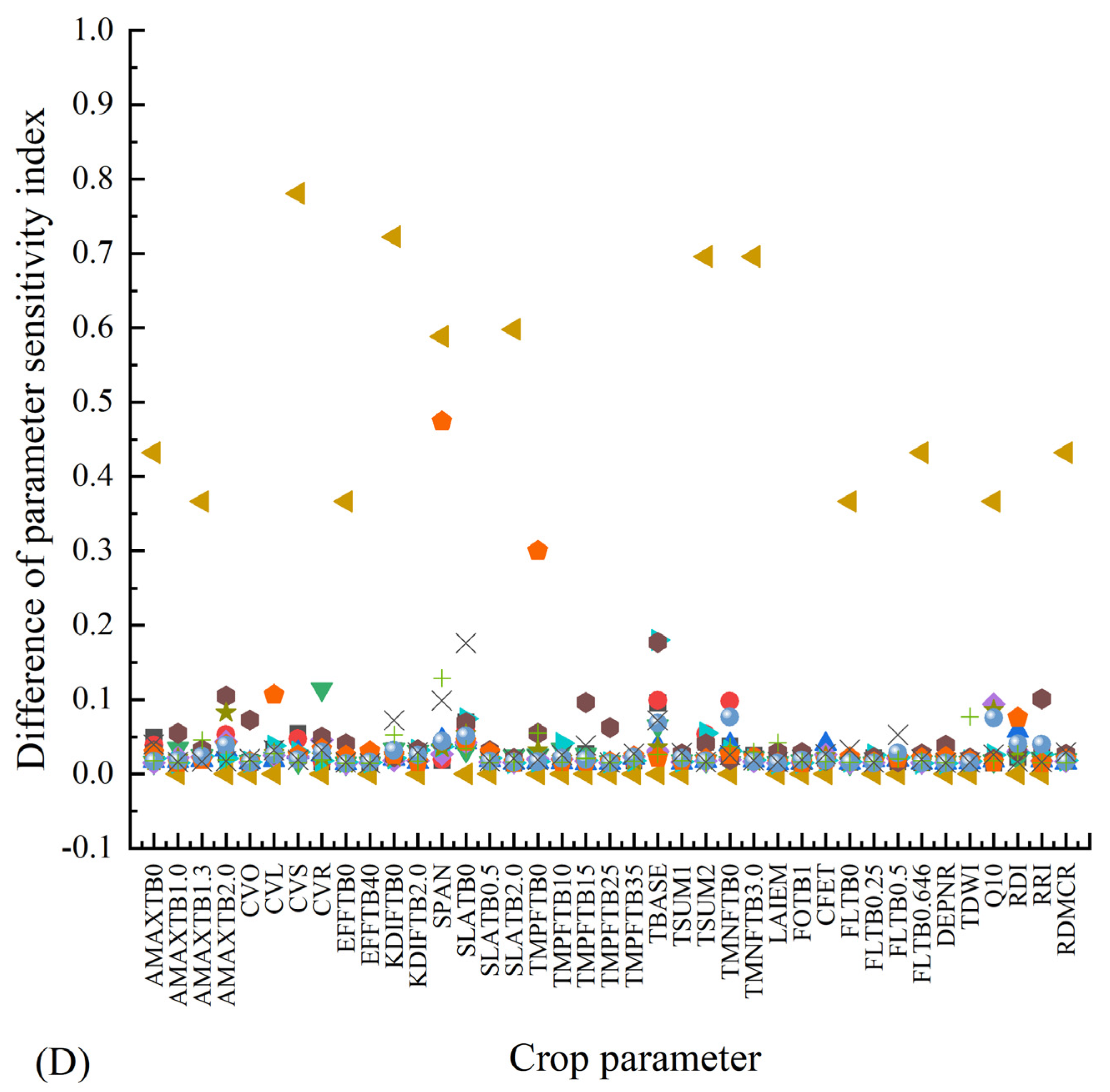
3.1. Spring Wheat Crop Parameter Sensitivity
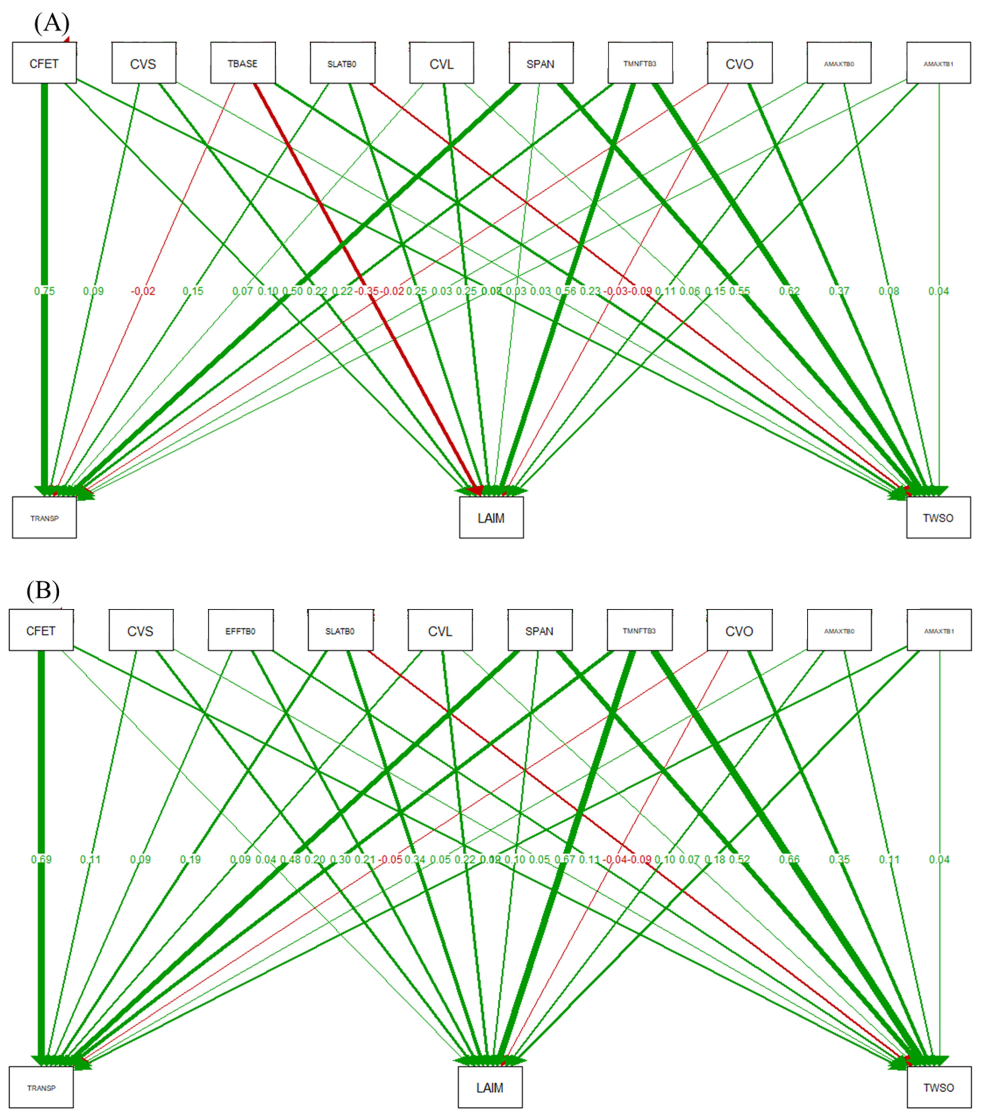
3.2. SEM of Degree of Contribution of Crop Parameters to Different Simulation Indices
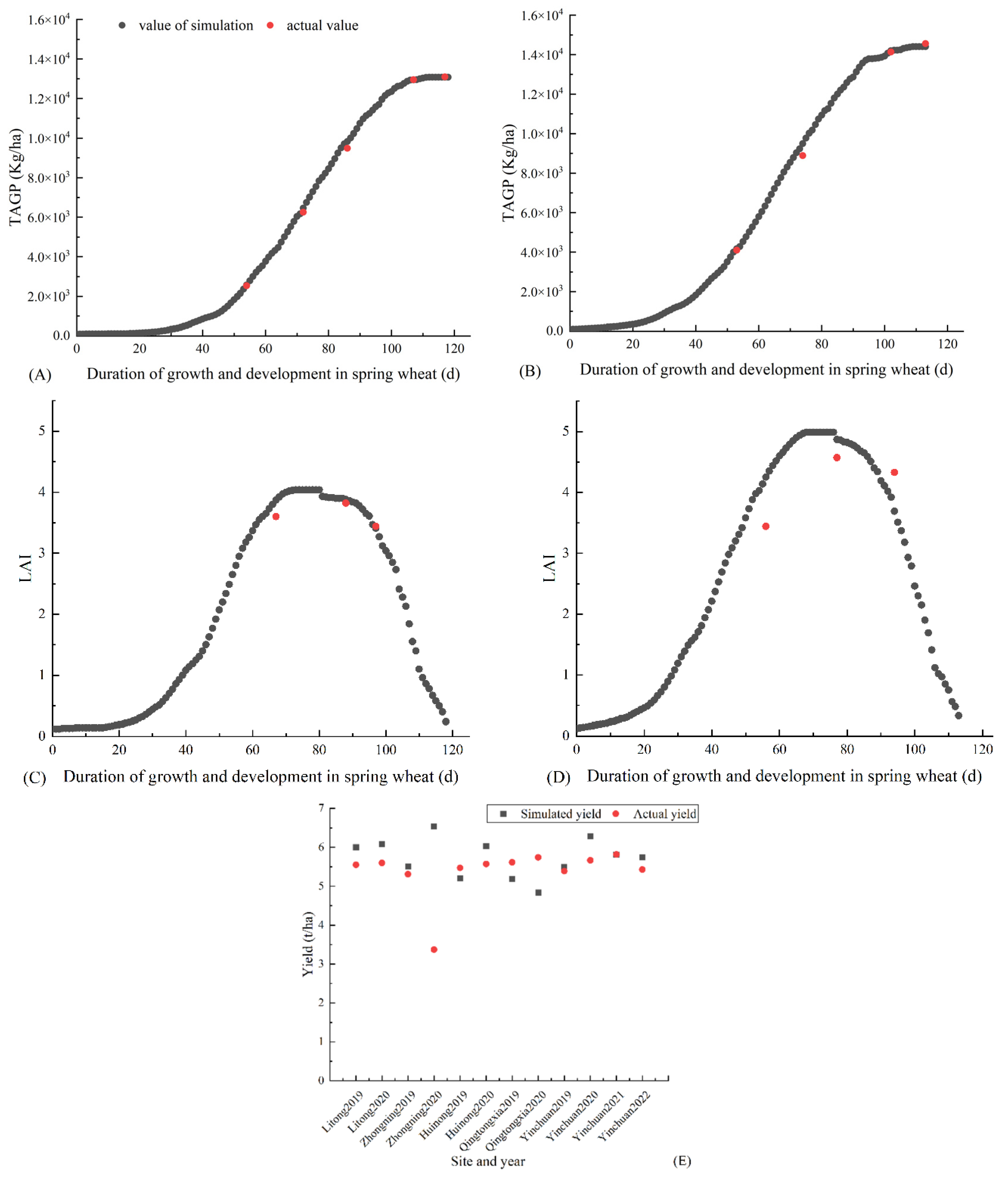
3.3. Adaptability Verification of the Modified WOFOST Model in the Ningxia Yellow River Irrigation Area
4. Discussion
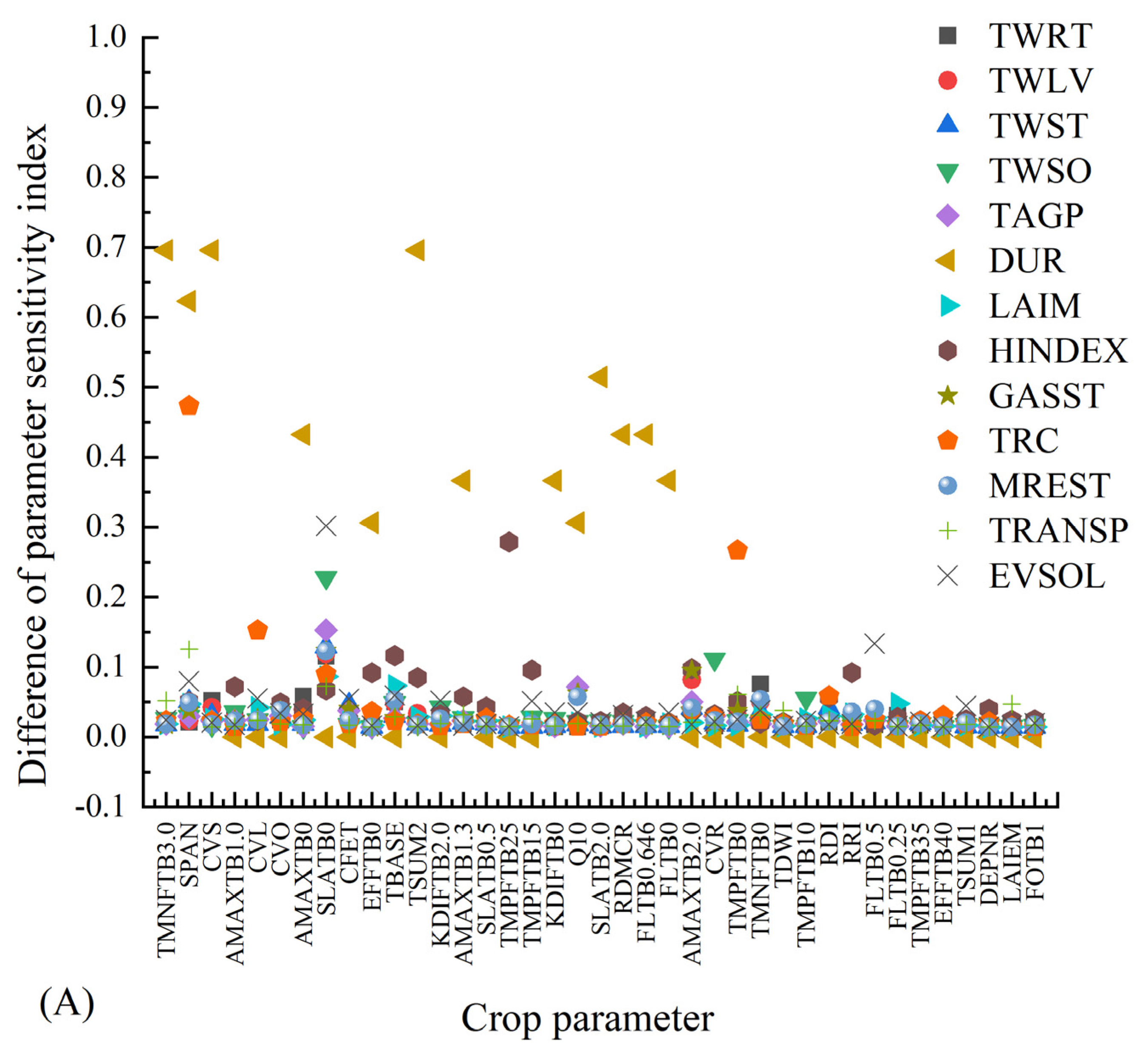
4.1. Analysis of Crop Parameter Sensitivity and its Response to Different Water Supply Conditions
4.2. Analysis of Degree of Contribution of SEM to Model Parameters
4.3. Localization of the WOFOST Model
5. Conclusions
- (1)
- The first-order and global sensitivity trends of spring wheat parameters in the WOFOST model showed consistent results. TMNFTB3.0, SPAN, SLATB0, and CFET exhibited higher sensitivity for most simulation indices. The impact of different water supply conditions on crop parameter sensitivity in the WOFOST model was limited under identical meteorological conditions. SA of crop parameters in the WOFOST model revealed that TMNFTB3.0, SPAN, CVS, AMAXTB1.0 and other crop parameters significantly affect the growth and development of spring wheat. Furthermore, water restriction severely impacted the growth-related indices, particularly leaf senescence, leaf area, and the assimilate allocation to storage organs.
- (2)
- The SEM identified CFET is the crop parameter with the highest contribution to the evapotranspiration index TRANSP, while TMNFTB3 have the highest impact on LAIM. TMNFTB3 is the most influential crop parameter for the yield index TWSO.
- (3)
- The TAGP simulation results from field trials conducted in Yongning County, Yinchuan City, during 2021 and 2022 met the model evaluation standards as evident from = 0.2516; = 0.1392; = 0.9976. For LAI results from the same field trials, the model evaluation standards were: = 0.4533; = 0.1283; = 0.2877. Therefore, the corrected model demonstrates improved simulation accuracy for the Ningxia Yellow River diversion irrigation area, with errors <8%.
Author Contributions
Funding
Data Availability Statement
Conflicts of Interest
Appendix A

| Water Supply Conditions and Meteorological Conditions | Total Root Dry Weight | Total Leaf Dry Weight | Total Stem Weight | Storage Organ Dry Weight | Total Above-Ground Production | Yield-Related Index | Simulated Time | Maximum Leaf Area Index | Harvest Index | Total Assimilation | Growth- Related Index | Transpiration Rate Coefficient | Total Maintenance Respiration | Total Transpiration | Total Surface Evaporation | Evapotranspiration Related Index | |||||||||||||
|---|---|---|---|---|---|---|---|---|---|---|---|---|---|---|---|---|---|---|---|---|---|---|---|---|---|---|---|---|---|
| First-Order Sensitivity Index of TWRT | Global Sensitivity Index of TWRT | First-Order Sensitivity Index of TWLV | Global Sensitivity Index of TWLV | First-Order Sensitivity Index of TWST | Global Sensitivity Index of TWST | First-Order Sensitivity Index of TWSO | Global Sensitivity Index of TWSO | First-Order Sensitivity index of TAGP | Global Sensitivity Index of TAGP | First-Order Sensitivity Index of DUR | Global Sensitivity Index of DUR | First-Order Sensitivity Index of LAIM | Global Sensitivity Index of LAIM | First-Order Sensitivity Index of HINDEX | Global Sensitivity Index of HINDEX | First-Order Sensitivity Index of GASST | The Global Sensitivity Index of GASST | First-ORDER Sensitivity Index of TRC | Global Sensitivity Index of TRC | First-Order Sensitivity Index of MREST | Global Sensitivity Index of MREST | First-order Sensitivity Index of TRANSP | Global Sensitivity Index of TRANSP | First-Order Sensitivity Index of EVSOL | Global Sensitivity Index of EVSOL | ||||
| Potential condition of 2021 | CVS | CVS | TMNFTB3.0 | TMNFTB3.0 | CVS | CVS | SPAN | SPAN | TMNFTB3.0 | TMNFTB3.0 | TMNFTB3.0 | SPAN | SPAN | TMNFTB3.0 | CVL | CVO | CVO | TMNFTB3.0 | TMNFTB3.0 | TMNFTB3.0 | TMNFTB3.0 | TMNFTB3.0 | TMNFTB3.0 | TMNFTB3.0 | CFET | CFET | SPAN | SPAN | TMNFTB3.0 |
| AMAXTB0 | AMAXTB0 | CVS | CVS | TMNFTB3.0 | TMNFTB3.0 | TMNFTB3.0 | TMNFTB3.0 | AMAXTB1.0 | AMAXTB1.0 | CVS | TMNFTB3.0 | TMNFTB3.0 | CVL | TMNFTB3.0 | SPAN | SPAN | AMAXTB1.0 | AMAXTB1.0 | SPAN | CFET | CFET | SPAN | SPAN | TMNFTB3.0 | TMNFTB3.0 | SLATB0 | SLATB0 | SPAN | |
| TMNFTB3.0 | TMNFTB3.0 | AMAXTB1.0 | AMAXTB1.0 | AMAXTB1.0 | AMAXTB1.0 | CVO | SLATB0 | SPAN | SPAN | AMAXTB1.0 | CVS | CVS | SLATB0.5 | SLATB0.5 | TMPFTB25 | TMPFTB25 | SPAN | SPAN | CVO | EFFTB0 | SPAN | AMAXTB1.0 | AMAXTB1.0 | SPAN | SPAN | CVL | CVL | CFET | |
| CVL | CVL | AMAXTB0 | AMAXTB0 | CVL | SLATB0 | KDIFTB2.0 | KDIFTB2.0 | CVS | SLATB0 | SPAN | TSUM2 | TSUM2 | CVS | SLATB0 | TBASE | TBASE | CVL | SLATB0 | CVS | CVL | CVL | CVL | SLATB0 | SLATB0 | SLATB0 | KDIFTB2.0 | KDIFTB2.0 | SLATB0 | |
| AMAXTB1.0 | AMAXTB1.0 | CVL | CVL | AMAXTB0 | CVL | AMAXTB1.0 | CVO | CVL | CVS | AMAXTB0 | SLATB2.0 | SLATB2.0 | AMAXTB0 | TBASE | AMAXTB1.3 | AMAXTB1.3 | AMAXTB0 | AMAXTB2.0 | AMAXTB1.0 | SPAN | TMPFTB0 | CVS | CVL | TDWI | TDWI | TMNFTB3.0 | TMNFTB3.0 | CVL | |
| Water restriction condition of 2021 | CVS | CVS | TMNFTB3.0 | TMNFTB3.0 | CVS | CVS | SPAN | SPAN | TMNFTB3.0 | TMNFTB3.0 | TMNFTB3.0 | SPAN | SPAN | TMNFTB3.0 | CVL | CVO | CVO | TMNFTB3.0 | TMNFTB3.0 | TMNFTB3.0 | TMNFTB3.0 | TMNFTB3.0 | TMNFTB3.0 | TMNFTB3.0 | CFET | CFET | SPAN | SPAN | TMNFTB3.0 |
| AMAXTB0 | AMAXTB0 | CVS | CVS | TMNFTB3.0 | TMNFTB3.0 | TMNFTB3.0 | TMNFTB3.0 | AMAXTB1.0 | AMAXTB1.0 | CVS | SLATB0 | SLATB0 | CVL | TMNFTB3.0 | SPAN | SPAN | AMAXTB1.0 | AMAXTB1.0 | SPAN | CFET | CFET | SPAN | SPAN | TMNFTB3.0 | TMNFTB3.0 | SLATB0 | SLATB0 | SPAN | |
| TMNFTB3.0 | TMNFTB3.0 | AMAXTB1.0 | AMAXTB1.0 | AMAXTB1.0 | AMAXTB1.0 | KDIFTB2.0 | KDIFTB2.0 | SPAN | SPAN | AMAXTB1.0 | KDIFTB0 | KDIFTB0 | SLATB0.5 | SLATB0.5 | TMPFTB25 | TMPFTB25 | SPAN | SPAN | CVO | EFFTB0 | SPAN | AMAXTB1.0 | AMAXTB1.0 | SPAN | SPAN | CVL | CVL | CFET | |
| CVL | CVL | AMAXTB0 | AMAXTB0 | CVL | CVL | CVO | CVO | CVS | CVS | SPAN | TMNFTB3.0 | TMNFTB3.0 | CVS | SLATB0 | TBASE | TBASE | CVL | AMAXTB2.0 | SLATB0 | CVL | CVL | CVL | CVL | TDWI | SLATB0 | KDIFTB2.0 | KDIFTB2.0 | CVL | |
| AMAXTB1.0 | AMAXTB1.0 | CVL | CVL | AMAXTB0 | SLATB0 | AMAXTB1.0 | CVR | CVL | CVL | AMAXTB0 | CVS | CVS | AMAXTB0 | TBASE | AMAXTB1.3 | AMAXTB1.3 | AMAXTB0 | SLATB0 | CVS | SPAN | TMPFTB0 | CVS | CVS | CVL | TDWI | TMNFTB3.0 | TMNFTB3.0 | SLATB0 | |
| Potential condition of 2022 | TMNFTB3.0 | TMNFTB3.0 | TMNFTB3.0 | TMNFTB3.0 | TMNFTB3.0 | TMNFTB3.0 | SPAN | SPAN | TMNFTB3.0 | TMNFTB3.0 | TMNFTB3.0 | SPAN | KDIFTB0 | TBASE | TBASE | CVO | CVO | TMNFTB3.0 | TMNFTB3.0 | TMNFTB3.0 | TMNFTB3.0 | TMNFTB3.0 | TMNFTB3.0 | TMNFTB3.0 | CFET | CFET | SPAN | SPAN | TMNFTB3.0 |
| CVL | CVS | CVS | CVS | CVS | CVS | TMNFTB3.0 | TMNFTB3.0 | AMAXTB1.0 | AMAXTB1.0 | CVS | KDIFTB0 | CVS | TMNFTB3.0 | TMNFTB3.0 | SPAN | SPAN | AMAXTB1.0 | AMAXTB1.0 | SPAN | CFET | CFET | SPAN | SPAN | TMNFTB3.0 | TMNFTB3.0 | SLATB0 | SLATB0 | SPAN | |
| CVS | CVL | AMAXTB0 | AMAXTB0 | AMAXTB1.0 | AMAXTB1.0 | CVO | CVO | SPAN | SPAN | SPAN | CVS | TDWI | SLATB0.5 | SLATB0.5 | TBASE | TBASE | SPAN | SPAN | CVO | CVL | SPAN | AMAXTB1.0 | AMAXTB1.0 | SPAN | TDWI | TMNFTB3.0 | KDIFTB0 | CFET | |
| AMAXTB0 | AMAXTB0 | CVL | TBASE | CVL | RDI | KDIFTB2.0 | KDIFTB2.0 | CVS | Q10 | AMAXTB1.0 | TDWI | SPAN | CVL | CVL | TMPFTB25 | TMPFTB25 | KDIFTB2.0 | KDIFTB2.0 | TBASE | EFFTB0 | TMPFTB0 | CVS | Q10 | TDWI | SPAN | KDIFTB0 | TMNFTB3.0 | SLATB0 | |
| TMPFTB15 | TBASE | TBASE | CVL | TBASE | TBASE | AMAXTB1.0 | TBASE | CVL | CVS | CVL | TMNFTB3.0 | TMNFTB3.0 | CVS | SLATB0 | AMAXTB1.3 | TMPFTB15 | AMAXTB0 | Q10 | CVS | SPAN | CVL | CVL | CVS | CVL | TMPFTB0 | KDIFTB2.0 | KDIFTB2.0 | CVL | |
| Water restriction condition of 2022 | TMNFTB3.0 | TMNFTB3.0 | TMNFTB3.0 | TMNFTB3.0 | TMNFTB3.0 | TMNFTB3.0 | SPAN | SPAN | TMNFTB3.0 | TMNFTB3.0 | TMNFTB3.0 | SPAN | SPAN | TBASE | TBASE | CVO | CVO | TMNFTB3.0 | TMNFTB3.0 | TMNFTB3.0 | TMNFTB3.0 | TMNFTB3.0 | TMNFTB3.0 | TMNFTB3.0 | CFET | CFET | SPAN | SPAN | TMNFTB3.0 |
| CVL | CVS | CVS | CVS | CVS | CVS | TMNFTB3.0 | TMNFTB3.0 | AMAXTB1.0 | AMAXTB1.0 | CVS | CVS | CVS | TMNFTB3.0 | TMNFTB3.0 | SPAN | SPAN | AMAXTB1.0 | AMAXTB1.0 | SPAN | CFET | CFET | SPAN | SPAN | TMNFTB3.0 | TMNFTB3.0 | SLATB0 | SLATB0 | SPAN | |
| CVS | CVL | AMAXTB0 | AMAXTB0 | AMAXTB1.0 | AMAXTB1.0 | CVO | CVO | SPAN | SPAN | SPAN | TMNFTB3.0 | KDIFTB0 | SLATB0.5 | SLATB0.5 | TBASE | TBASE | SPAN | SPAN | CVO | CVL | SPAN | AMAXTB1.0 | AMAXTB1.0 | SPAN | SPAN | TMNFTB3.0 | KDIFTB0 | CFET | |
| AMAXTB0 | AMAXTB0 | CVL | TBASE | CVL | RDI | KDIFTB2.0 | KDIFTB2.0 | CVS | Q10 | AMAXTB1.0 | TSUM2 | TMNFTB3.0 | CVL | CVL | TMPFTB25 | TMPFTB25 | KDIFTB2.0 | KDIFTB2.0 | TBASE | EFFTB0 | TMPFTB0 | CVS | Q10 | TDWI | TDWI | KDIFTB0 | TMNFTB3.0 | CVL | |
| TMPFTB15 | TBASE | TBASE | CVL | TBASE | TBASE | AMAXTB1.0 | TBASE | CVL | CVS | CVL | KDIFTB0 | TSUM2 | CVS | SLATB0 | AMAXTB1.3 | TMPFTB15 | AMAXTB0 | Q10 | CVS | SPAN | CVL | CVL | CVS | CVL | TMPFTB0 | KDIFTB2.0 | KDIFTB2.0 | SLATB0 | |
| Abbreviations | Meaning | Abbreviations | Meaning | Abbreviations | Meaning |
|---|---|---|---|---|---|
| EFAST | Extended Fourier Amplitude Sensitivity Test | SWM | soil moisture content at the wilting point | TAGP | total aboveground production |
| WOFOST | World Food Studies Simulation | DVS | developmental stages of crops | DUR | growth time |
| SEM | Structural Equation Model | SMFCF | the soil moisture content at field capacity | LAIM | maximum leaf area index |
| CERES | Crop Environment Resource Synthesis | SM0 | the soil moisture content at saturation | HINDEX | Harvest index |
| APSIM | Agricultural Production Systems sIMulator | K0 | hydraulic conductivity of saturated soil | GASST | total assimilation |
| DSSAT | Decision Support System for Agrotechnology Transfer | TWRT | total root dry weight | TRC | transpiration coefficient rate |
| Root-mean-square error | TWLV | total leaf dry weight | MREST | total maintenance respiration | |
| Mean bias error | TWST | total stem dry weight | TRANSP | total transpiration | |
| determination coefficient | TWSO | storage organ dry weight | EVSOL | total evaporation from the soil surface |
References
- Zhao, J.; Pu, F.; Li, Y.; Xu, J.; Li, N.; Zhang, Y.; Guo, J.; Pan, Z. Assessing the combined effects of climatic factors on spring wheat phenophase and grain yield in inner mongolia, China. PLoS ONE 2017, 12, e185690. [Google Scholar] [CrossRef]
- Osborne, T.M.; Lawrence, D.M.; Challinor, A.J.; Slingo, J.M.; Wheeler, T.R. Development and assessment of a coupled crop–climate model. Glob. Chang. Biol. 2007, 13, 169–183. [Google Scholar] [CrossRef]
- Bowerman, A.F.; Newberry, M.; Dielen, A.; Whan, A.; Larroque, O.; Pritchard, J.; Gubler, F.; Howitt, C.A.; Pogson, B.J.; Morell, M.K.; et al. Suppression of glucan, water dikinase in the endosperm alters wheat grain properties, germination and coleoptile growth. Plant Biotechnol. J. 2016, 14, 398–408. [Google Scholar] [CrossRef] [PubMed]
- Zhai, Z.; Martínez, J.F.; Beltran, V.; Martínez, N.L. Decision support systems for agriculture 4.0: Survey and challenges. Comput. Electron. Agric. 2020, 170, 105256. [Google Scholar] [CrossRef]
- Gaydon, D.S.; Balwinder-Singh Wang, E.; Poulton, P.L.; Ahmad, B.; Ahmed, F.; Akhter, S.; Ali, I.; Amarasingha, R.; Chaki, A.K.; Chen, C.; et al. Evaluation of the apsim model in cropping systems of Asia. Field Crops Res. 2017, 204, 52–75. [Google Scholar] [CrossRef]
- Ceglar, A.; van der Wijngaart, R.; de Wit, A.; Lecerf, R.; Boogaard, H.; Seguini, L.; van den Berg, M.; Toreti, A.; Zampieri, M.; Fumagalli, D.; et al. Improving wofost model to simulate winter wheat phenology in europe: Evaluation and effects on yield. Agric. Syst. 2019, 168, 168–180. [Google Scholar] [CrossRef]
- Leghari, S.J.; Hu, K.; Liang, H.; Wei, Y. Modeling water and nitrogen balance of different cropping systems in the north China plain. Agronomy 2019, 9, 696. [Google Scholar] [CrossRef]
- Shahhosseini, M.; Hu, G.; Huber, I.; Archontoulis, S.V. Coupling machine learning and crop modeling improves crop yield prediction in the us corn belt. Sci. Rep. 2021, 11, 1606. [Google Scholar] [CrossRef]
- Zhang, Y.; Li, S.; Wu, M.; Yang, D.; Wang, C. Study on the response of different soybean varieties to water management in northwest China based on a model approach. Atmosphere 2021, 12, 824. [Google Scholar] [CrossRef]
- Bregaglio, S.; Donatelli, M.; Confalonieri, R.; Acutis, M.; Orlandini, S. Multi metric evaluation of leaf wetness models for large-area application of plant disease models. Agric. For. Meteorol. 2011, 151, 1163–1172. [Google Scholar] [CrossRef]
- Heng, L.K.; Hsiao, T.; Evett, S.; Howell, T.; Steduto, P. Validating the fao aquacrop model for irrigated and water deficient field maize. Agron. J. 2009, 101, 488–498. [Google Scholar] [CrossRef]
- Liang, H.; Hu, K.; Batchelor, W.D.; Qin, W.; Li, B. Developing a water and nitrogen management model for greenhouse vegetable production in China: Sensitivity analysis and evaluation. Ecol. Model. 2018, 367, 24–33. [Google Scholar] [CrossRef]
- Makler-Pick, V.; Gal, G.; Gorfine, M.; Hipsey, M.R.; Carmel, Y. Sensitivity analysis for complex ecological models—A new approach. Environ. Model. Softw. 2011, 26, 124–134. [Google Scholar] [CrossRef]
- Stella, T.; Frasso, N.; Negrini, G.; Bregaglio, S.; Cappelli, G.; Acutis, M.; Confalonieri, R. Model simplification and development via reuse, sensitivity analysis and composition: A case study in crop modelling. Environ. Model. Softw. 2014, 59, 44–58. [Google Scholar] [CrossRef]
- Tan, J.; Cui, Y.; Luo, Y. Global sensitivity analysis of outputs over rice-growth process in Oryza model. Environ. Model. Softw. 2016, 83, 36–46. [Google Scholar] [CrossRef]
- Corbeels, M.; Chirat, G.; Messad, S.; Thierfelder, C. Performance and sensitivity of the dssat crop growth model in simulating maize yield under conservation agriculture. Eur. J. Agron. 2016, 76, 41–53. [Google Scholar] [CrossRef]
- Tao, S.; Shen, S.; Li, Y.; Wang, Q.; Gao, P.; Mugume, I. Projected crop production under regional climate change using scenario data and modeling: Sensitivity to chosen sowing date and cultivar. Sustainability 2016, 8, 214. [Google Scholar] [CrossRef]
- Ojeda, J.J.; Volenec, J.J.; Brouder, S.M.; Caviglia, O.P.; Agnusdei, M.G. Evaluation of agricultural production systems simulator as yield predictor of Panicum virgatum and Miscanthus x giganteus in several us environments. Glob. Chang. Biol. Bioenergy 2017, 9, 796–816. [Google Scholar] [CrossRef]
- Borgonovo, E.; Plischke, E. Sensitivity analysis: A review of recent advances. Eur. J. Oper. Res. 2016, 248, 869–887. [Google Scholar] [CrossRef]
- Wallach, D.; Thorburn, P.J. Estimating uncertainty in crop model predictions: Current situation and future prospects. Eur. J. Agron. 2017, 88, A1–A7. [Google Scholar] [CrossRef]
- Varella, H.; Guérif, M.; Buis, S. Global sensitivity analysis measures the quality of parameter estimation: The case of soil parameters and a crop model. Environ. Model. Softw. 2010, 25, 310–319. [Google Scholar] [CrossRef]
- Abbate, P.E.; Dardanelli, J.L.; Cantarero, M.G.; Maturano, M.; Melchiori, R.J.M.; Suero, E.E. Climatic and water availability effects on water-use efficiency in wheat. Crop Sci. 2004, 44, 474–483. [Google Scholar] [CrossRef]
- Song, M.D.; Feng, H.; Li, Z.P.; Gao, J.E. Sensitivity analysis of ceres-wheat model based on morris and efast. Chin. J. Agric. Mach. 2014, 45, 124–131. [Google Scholar]
- Xiao, Y.; Zhao, W.; Zhou, D.; Gong, H. Sensitivity analysis of vegetation reflectance to biochemical and biophysical variables at leaf, canopy, and regional scales. IEEE Trans. Geosci. Remote Sens. 2014, 52, 4014–4024. [Google Scholar] [CrossRef]
- Sobol, I.M. Global sensitivity indices for nonlinear mathematical models and their Monte Carlo estimates. Math. Comput. Simul. 2001, 55, 271–280. [Google Scholar] [CrossRef]
- Cui, J.T.; Shao, G.C.; Lin, J.; Ding, M.M. Global sensitivity analysis of parameters of cropgro-tomato model based on efast. J. Agric. Mach. 2020, 51, 237–244. [Google Scholar]
- Wu, J.; Yu, F.S.; Chen, Z.X.; Chen, J. Global sensitivity analysis of winter wheat growth simulation parameters based on epic model. Chin. J. Agric. Eng. 2009, 25, 136–142. [Google Scholar]
- Wang, J.; Li, X.; Lu, L.; Fang, F. Parameter sensitivity analysis of crop growth models based on the extended Fourier amplitude sensitivity test method. Environ. Model. Softw. 2013, 48, 171–182. [Google Scholar] [CrossRef]
- Confalonieri, R. Monte Carlo based sensitivity analysis of two crop simulators and considerations on model balance. Eur. J. Agron. 2010, 33, 89–93. [Google Scholar] [CrossRef]
- Dejonge, K.C.; Ascough, J.C.; Ahmadi, M.; Andales, A.A.; Arabi, M. Global sensitivity and uncertainty analysis of a dynamic agroecosystem model under different irrigation treatments. Ecol. Model. 2012, 231, 113–125. [Google Scholar] [CrossRef]
- Lei, G.; Zeng, W.; Jiang, Y.; Ao, C.; Wu, J.; Huang, J. Sensitivity analysis of the swap (soil-water-atmosphere-plant) model under different nitrogen applications and root distributions in saline soils. Pedosphere 2021, 31, 807–821. [Google Scholar] [CrossRef]
- Vanuytrecht, E.; Raes, D.; Steduto, P.; Hsiao, T.C.; Fereres, E.; Heng, L.K.; Garcia Vila, M.; Mejias Moreno, P. Aquacrop: Fao’s crop water productivity and yield response model. Environ. Model. Softw. 2014, 62, 351–360. [Google Scholar] [CrossRef]
- Brun, R.; Reichert, P.; Kuensch, H.R. Practical identifiability analysis of large environmental simulation models. Water Resour. Res. 2001, 37, 1015–1030. [Google Scholar] [CrossRef]
- Confalonieri, R.; Bellocchi, G.; Tarantola, S.; Acutis, M.; Donatelli, M.; Genovese, G. Sensitivity analysis of the rice model warm in europe: Exploring the effects of different locations, climates and methods of analysis on model sensitivity to crop parameters. Environ. Model. Softw. 2010, 25, 479–488. [Google Scholar] [CrossRef]
- Pastres, R.; Ciavatta, S. A comparison between the uncertainties in model parameters and in forcing functions: Its application to a 3D water-quality model. Environ. Model. Softw. 2005, 20, 981–989. [Google Scholar] [CrossRef]
- Wu, D.R.; Ouyang, Z.; Zhao, X.M.; Yu, Q.; Luo, Y. Applicability of crop growth model Wofost in North China Plain. Chin. J. Plant Ecol. 2003, 27, 594–602. [Google Scholar]
- Xie, W.X.; Wang, G.H.; Zhang, Q.C. Development and application of Wofost model. Chin. J. Soil Sci. 2006, 1, 154–158. [Google Scholar]
- Zhu, J.H.; Dai, P.; Zhu, K.Q.; Chen, Y.; Fan, Y.C.; Li, J.; Feng, D.L.; Qu, H.Q. Research progress of Wofost model. J. Anhui Agric. Sci. 2016, 44, 194–196. [Google Scholar]
- Wang, W.-B.; Wang, J.-M.; Fan, Y.-Y.; Chen, J.; Miles, D.; Jin, H.-J.; He, H.-L. Evaluation of simulation performance of soil water characteristic curve model. J. Glaciol. Geocryol. 2019, 41, 1448–1455. [Google Scholar]
- Schaap, M.G.; Leij, F.J.; van Genuchten, M.T. Rosetta: A computer program for estimating soil hydraulic parameters with hierarchical pedotransfer functions. J. Hydrol. 2001, 251, 163–176. [Google Scholar] [CrossRef]
- Wang, L.; Weng, X.; Yao, Z.; Zhang, R.; Li, W.; Li, Y. Segmental modification of the mualem model by remolded loess. Math. Probl. Eng. 2017, 2017, 2768952. [Google Scholar] [CrossRef]
- Esfandiari, A. An innovative sensitivity-based method for structural model updating using incomplete modal data. Struct. Control Health Monit. 2017, 24, e1905. [Google Scholar] [CrossRef]
- Amini, A.; Alimohammadlou, M. Toward equation structural modeling: An integration of interpretive structural modeling and structural equation modeling. J. Manag. Anal. 2021, 8, 693–714. [Google Scholar] [CrossRef]
- Grace, J.B.; Anderson, T.M.; Olff, H.; Scheiner, S.M. On the specification of structural equation models for ecological systems. Ecol. Monogr. 2010, 80, 67–87. [Google Scholar] [CrossRef]
- Chen, Y.L.; Gu, X.H.; Gong, A.D. Parameter sensitivity analysis of Wofost crop model based on efast method. J. Henan Polytech. Univ. 2018, 37, 72–78. [Google Scholar]
- He, L.; Hou, Y.Y.; Zhao, G.; Wu, D.R.; Yu, Q. Parameter optimization of Wofost crop model based on global sensitivity analysis and Bayesian method. Chin. J. Agric. Eng. 2016, 32, 169–179. [Google Scholar]
- Xing, A.; Zhuo, Z.Q.; Zhao, Y.Z.; Li, Y.; Huang, Y.F. Parameter sensitivity analysis of Wofost model at different production levels based on efast. Chin. J. Agric. Mach. 2020, 51, 161–171. [Google Scholar]
- Saltelli, A.; Tarantola, S.; Chan, K.P.S. A quantitative model-independent method for global sensitivity analysis of model output. Technometrics 1999, 41, 39. [Google Scholar] [CrossRef]
- Scollo, S.; Tarantola, S.; Bonadonna, C.; Coltelli, M.; Saltelli, A. Sensitivity analysis and uncertainty estimation for tephra dispersal models. J. Geophys. Res. 2008, 113, 4864. [Google Scholar] [CrossRef]
- Chan, I.S.; Goldstein, A.A.; Bassingthwaighte, J.B. Sensop: A derivative-free solver for nonlinear least squares with sensitivity scaling. Ann. Biomed. Eng. 1993, 21, 621–631. [Google Scholar] [CrossRef]
- Xing, H.; Xu, X.; Li, Z.; Chen, Y.; Feng, H.; Yang, G.; Chen, Z. Global sensitivity analysis of the aquacrop model for winter wheat under different water treatments based on the extended Fourier amplitude sensitivity test. J. Integr. Agric. 2017, 16, 2444–2458. [Google Scholar] [CrossRef]
- Dimov, I.; Georgieva, R.; Ostromsky, T. Monte Carlo sensitivity analysis of an Eulerian large-scale air pollution model. Reliab. Eng. Syst. Saf. 2012, 107, 23–28. [Google Scholar] [CrossRef]
- Li, Z.; Jin, X.; Liu, H.; Xu, X.; Wang, J. Global sensitivity analysis of wheat grain yield and quality and the related process variables from the dssat-ceres model based on the extended Fourier amplitude sensitivity test method. J. Integr. Agric. 2019, 18, 1547–1561. [Google Scholar] [CrossRef]
- Vazquez-Cruz, M.A.; Guzman-Cruz, R.; Lopez-Cruz, I.L.; Cornejo-Perez, O.; Torres-Pacheco, I.; Guevara-Gonzalez, R.G. Global sensitivity analysis by means of efast and sobol’ methods and calibration of reduced state-variable tomgro model using genetic algorithms. Comput. Electron. Agric. 2014, 100, 1–12. [Google Scholar] [CrossRef]
- Zhang, J.L.; Li, Y.P.; Zeng, X.T.; You, L.; Liu, J. Sensitivity analysis of hydrological process parameters in cold and arid regions based on efast method. S. N. Water Divers. Water Technol. 2017, 15, 43–48. [Google Scholar]
- Gao, J.; Zhou, B.P.; Wang, Y.; Wang, J.; Yu, H. Sensitivity analysis and applicability evaluation of efast based dssat model for cotton parameters in southern Xinjiang. Jiangsu Agric. Sci. 2022, 50, 185–191. [Google Scholar]
- Wang, J.D.; Guo, W.D.; Li, H.Q. Application of extended Fourier amplitude sensitivity test (efast) method in land surface parameter sensitivity analysis. Acta Phys. Sin. 2013, 62, 050202. [Google Scholar] [CrossRef]
- Wang, Z.M.; Zhang, B.; Song, K.S.; Duan, H.T. Calibration and validation of Cropsyst crop model in typical black soil area of Songnen Plain. J. Agric. Eng. 2005, 21, 47–50. [Google Scholar]
- Lv, L.; Liang, S.; Zhang, J.; Yao, Y.; Dong, Z.; Zhang, L.; Jia, X.-L. Response of yield and light use of different wheat varieties to accumulated temperature before winter. J. Wheat Crops 2017, 37, 1047–1055. [Google Scholar]
- Jin, H.; Li, A.; Wang, J.; Bo, Y. Improvement of spatially and temporally continuous crop leaf area index by integration of ceres-maize model and modis data. Eur. J. Agron. 2016, 78, 1–12. [Google Scholar] [CrossRef]
- Cheng, Z.; Meng, J.; Wang, Y. Improving spring maize yield estimation at field scale by assimilating time-series hj-1 ccd data into the wofost model using a new method with fast algorithms. Remote Sens. 2016, 8, 303. [Google Scholar] [CrossRef]
- Gilardelli, C.; Confalonieri, R.; Cappelli, G.A.; Bellocchi, G. Sensitivity of wofost-based modelling solutions to crop parameters under climate change. Ecol. Model. 2018, 368, 1–14. [Google Scholar] [CrossRef]
- Zhang, N.; Zhang, Q.G.; Yu, H.J.; Cheng, M.D.; Dong, S.J. Parametric sensitivity analysis of crop growth simulation models. J. Zhejiang Univ. (Agric. Life Sci.) 2018, 44, 107–115. [Google Scholar]
- Xu, X.; Shen, S.; Xiong, S.; Ma, X.; Fan, Z.; Han, H. Water stress is a key factor influencing the parameter sensitivity of the wofost model in different agro-meteorological conditions. Int. J. Plant Prod. 2021, 15, 231–242. [Google Scholar] [CrossRef]
- Bassu, S.; Brisson, N.; Durand, J.; Boote, K.; Lizaso, J.; Jones, J.W.; Rosenzweig, C.; Ruane, A.C.; Adam, M.; Baron, C.; et al. How do various maize crop models vary in their responses to climate change factors? Glob. Chang. Biol. 2014, 20, 2301–2320. [Google Scholar] [CrossRef]
- Constantin, J.; Raynal, H.; Casellas, E.; Hoffmann, H.; Bindi, M.; Doro, L.; Eckersten, H.; Gaiser, T.; Grosz, B.; Haas, E.; et al. Management and spatial resolution effects on yield and water balance at regional scale in crop models. Agric. For. Meteorol. 2019, 275, 184–195. [Google Scholar] [CrossRef]
- Wu, J.; Gu, Y.; Sun, K.; Wang, N.; Shen, H.; Wang, Y.; Ma, X. Correlation of climate change and human activities with agricultural drought and its impact on the net primary production of winter wheat. J. Hydrol. 2023, 620, 129504. [Google Scholar] [CrossRef]
- Dewitt, N.; Guedira, M.; Murphy, J.P.; Marshall, D.; Mergoum, M.; Maltecca, C.; Brown-Guedira, G. A network modeling approach provides insights into the environment-specific yield architecture of wheat. Genetics 2022, 221, iyac076. [Google Scholar] [CrossRef]
- Vargas, M.; Crossa, J.; Reynolds, M.P.; Dhungana, P.; Eskridge, K.M. Paper presented at international workshop on increasing wheat yield potential, Cimmyt, Obregon, Mexico, 20–24 March 2006 structural equation modelling for studying genotype × environment interactions of physiological traits affecting yield in wheat. J. Agric. Sci. 2007, 145, 151. [Google Scholar] [CrossRef]
- Mishra, V.; Cruise, J.F.; Mecikalski, J.R. Assimilation of coupled microwave/thermal infrared soil moisture profiles into a crop model for robust maize yield estimates over southeast united states. Eur. J. Agron. 2021, 123, 126208. [Google Scholar] [CrossRef]
- Zinyengere, N.; Crespo, O.; Hachigonta, S.; Tadross, M. Local impacts of climate change and agronomic practices on dry land crops in southern africa. Agric. Ecosyst. Environ. 2014, 197, 1–10. [Google Scholar] [CrossRef]
- Horton, R.M.; Mankin, J.S.; Lesk, C.; Coffel, E.; Raymond, C. A review of recent advances in research on extreme heat events. Curr. Clim. Chang. Rep. 2016, 2, 242–259. [Google Scholar] [CrossRef]
- Gabrielle, B.; Laville, P.; Duval, O.; Nicoullaud, B.; Germon, J.C.; Hénault, C. Process-based modeling of nitrous oxide emissions from wheat-cropped soils at the subregional scale. Glob. Biogeochem. Cycles 2006, 20. [Google Scholar] [CrossRef]


| Research Area | Organic Carbon Content/(g·kg−1) | Crushed Stone Volume/% | Sand Content/% | Silt Content/% | Clay Content/% | Soil Bulk Density/g·cm−3 | PH Value |
|---|---|---|---|---|---|---|---|
| Yinchuan | 1.12 | 10 | 29 | 50 | 21 | 1.38 | 7.8 |
| Litong | 0.46 | 7 | 41 | 38 | 21 | 1.4 | 8.1 |
| Zhongning | 1.12 | 10 | 34 | 45 | 21 | 1.39 | 7.9 |
| Huinong | 0.46 | 7 | 41 | 38 | 21 | 1.4 | 8.1 |
| Qingtongxia | 1.12 | 10 | 29 | 50 | 21 | 1.38 | 7.8 |
| Parameter | Significance | Unit | Lower Limiting Value | Upper Limiting Value | Parameter | Significance | Unit | Lower Limiting Value | Upper Limiting Value |
|---|---|---|---|---|---|---|---|---|---|
| AMAXTB0 | Maximum CO2 assimilation rate under DVS = 0 | kg·hm−2·h−1 | 32.247 | 39.413 | TMPFTB35 | Correction factor of maximum assimilation rate under mean temperature 25 °C | 0 | 0.1 | |
| AMAXTB1.0 | Maximum CO2 assimilation rate under DVS = 1.0 | kg·hm−2·h−1 | 32.247 | 39.413 | TBASE | Lower threshold temperature for emergence | −2 | 2 | |
| AMAXTB1.3 | Maximum CO2 assimilation rate under DVS = 1.3 | kg·hm−2·h−1 | 32.247 | 39.413 | TSUM1 | Cumulative Temperature from emergence to flowering | °C·d | 800 | 1500 |
| AMAXTB2.0 | Maximum CO2 assimilation rate under DVS = 2.0 | kg·hm−2·h−1 | 4.032 | 4.928 | TSUM2 | Cumulative Temperature from flowering to maturity | °C·d | 600 | 1350 |
| CVO | Efficiency of conversion into storage organs | kg·kg−1 | 0.6381 | 0.7799 | TMNFTB0 | Correction factor of total assimilation rate under minimum temperature 0 °C | 0 | 0.1 | |
| CVL | Efficiency of conversion into leaves | kg·kg−1 | 0.6165 | 0.7535 | TMNFTB30 | Correction factor of total assimilation rate under minimum temperature 0 °C | 0.9 | 1.1 | |
| CVS | Efficiency of conversion into stems | kg·kg−1 | 0.63 | 0.7282 | LAIEM | Leaf area index at emergence | hm2·hm−2 | 0.12285 | 0.15015 |
| CVR | Efficiency of conversion into roots | kg·kg−1 | 0.65 | 0.7634 | FOTB1 | The dry matter distribution coefficient of storage organs increased under DVS = 1 | kg·kg−1 | 0.9 | 1.1 |
| EFFTB0 | Light energy utilization rate of single leaf under average daily temperature 0 °C | kg·hm−2·h−1·J−1·m2·s | 0.405 | 0.495 | CFET | Correction factor transpiration rate | 0.9 | 1.1 | |
| EFFTB40 | Light energy utilization rate of single leaf under average daily temperature 40 °C | kg·hm−2·h−1·J−1·m2·s | 0.405 | 0.495 | FLTB0 | Leaf dry matter distribution coefficient under DVS = 0 | kg·kg−1 | 0.585 | 0.715 |
| KDIFTB0 | Extinction coefficient for diffuse visible light under DVS = 0 | 0.54 | 0.66 | FLTB0.25 | Leaf dry matter distribution coefficient under DVS = 0.25 | kg·kg−1 | 0.63 | 0.77 | |
| KDIFTB2.0 | Extinction coefficient for diffuse visible light under DVS = 2.0 | 0.54 | 0.66 | FLTB0.5 | Leaf dry matter distribution coefficient under DVS = 0.5 | kg·kg−1 | 0.45 | 0.55 | |
| SPAN | Life span of leaves growing at 35 Celsius | d | 28.17 | 34.43 | FLTB0.646 | Leaf dry matter distribution coefficient under DVS = 0.646 | kg·kg−1 | 0.27 | 0.33 |
| SLATB0 | Specific leaf area under DVS = 0 | hm2·kg−1 | 0.001908 | 0.002332 | DEPNR | Crop group number for soil water depletion | 4.05 | 4.95 | |
| SLATB0.5 | Specific leaf area under DVS = 0.5 | hm2·kg−1 | 0.001908 | 0.002332 | TDWI | Initial total crop dry weight | kg·hm−2 | 180 | 220 |
| SLATB2.0 | Specific leaf area under DVS = 2.0 | hm2·kg−1 | 0.001908 | 0.002332 | Q10 | Relative change in respiratory rate for every 10 °C temperature change | 1.8 | 2 | |
| TMPFTB0 | Correction factor of maximum assimilation rate under mean temperature 0 °C | 0.009 | 0.1 | RDI | Initial rooting depth | cm | 10 | 12 | |
| TMPFTB10 | Correction factor of maximum assimilation rate under mean temperature 0 °C | 0.54 | 1 | RRI | Maximum daily increase in rooting depth | cm·d−1 | 1.08 | 1.32 | |
| TMPFTB15 | Correction factor of maximum assimilation rate under mean temperature 15 °C | 0.9 | 1 | RDMCR | Maximum rooting depth | cm | 112.5 | 137.5 | |
| TMPFTB25 | Correction factor of maximum assimilation rate under mean temperature 25 °C | 0.9 | 1 |
| Crop Parameter | Value | Crop Parameter | Value | Crop Parameter | Value | Crop Parameter | Value |
|---|---|---|---|---|---|---|---|
| AMAXTB0 | 35.2528 | CVS | 0.724642 | KDIFTB2 | 0.654335 | TMPFTB0 | 0.099835 |
| AMAXTB1 | 39.0031 | CVR | 0.667882 | SPAN | 33.0204 | TMPFTB10 | 0.56683 |
| AMAXTB1.3 | 38.1757 | EFFTB0 | 0.487338 | SLATB0 | 0.002004 | TMPFTB15 | 0.937174 |
| CVO | 0.765686 | EFFTB40 | 0.476887 | SLATB0.5 | 0.001944 | TMPFTB25 | 0.956712 |
| CVL | 0.667321 | KDIFTB0 | 0.573685 | SLATB2 | 0.002072 | TMPFTB35 | 0.015039 |
| TBASE | −1.53077 | LAIEM | 0.129034 | FLTB0.5 | 0.450768 | RDI | 11.9468 |
| TSUM1 | 1269.89 | FOTB1 | 0.956577 | FLTB0.646 | 0.296593 | RRI | 1.29025 |
| TSUM2 | 1263.68 | CFET | 0.929755 | DEPNR | 4.64869 | RDMCR | 122.543 |
| TMNFTB0 | 0.078391 | FLTB0 | 0.601276 | TDWI | 182.62 | AMAXTB2 | 4.84661 |
| TMNFTB3 | 0.913048 | FLTB0.25 | 0.641849 | Q10 | 1.87027 |
Disclaimer/Publisher’s Note: The statements, opinions and data contained in all publications are solely those of the individual author(s) and contributor(s) and not of MDPI and/or the editor(s). MDPI and/or the editor(s) disclaim responsibility for any injury to people or property resulting from any ideas, methods, instructions or products referred to in the content. |
© 2023 by the authors. Licensee MDPI, Basel, Switzerland. This article is an open access article distributed under the terms and conditions of the Creative Commons Attribution (CC BY) license (https://creativecommons.org/licenses/by/4.0/).
Share and Cite
Li, X.; Tan, J.; Li, H.; Wang, L.; Niu, G.; Wang, X. Sensitivity Analysis of the WOFOST Crop Model Parameters Using the EFAST Method and Verification of Its Adaptability in the Yellow River Irrigation Area, Northwest China. Agronomy 2023, 13, 2294. https://doi.org/10.3390/agronomy13092294
Li X, Tan J, Li H, Wang L, Niu G, Wang X. Sensitivity Analysis of the WOFOST Crop Model Parameters Using the EFAST Method and Verification of Its Adaptability in the Yellow River Irrigation Area, Northwest China. Agronomy. 2023; 13(9):2294. https://doi.org/10.3390/agronomy13092294
Chicago/Turabian StyleLi, Xinlong, Junli Tan, Hong Li, Lili Wang, Guoli Niu, and Xina Wang. 2023. "Sensitivity Analysis of the WOFOST Crop Model Parameters Using the EFAST Method and Verification of Its Adaptability in the Yellow River Irrigation Area, Northwest China" Agronomy 13, no. 9: 2294. https://doi.org/10.3390/agronomy13092294
APA StyleLi, X., Tan, J., Li, H., Wang, L., Niu, G., & Wang, X. (2023). Sensitivity Analysis of the WOFOST Crop Model Parameters Using the EFAST Method and Verification of Its Adaptability in the Yellow River Irrigation Area, Northwest China. Agronomy, 13(9), 2294. https://doi.org/10.3390/agronomy13092294