Abstract
Applying the correct dose of nitrogen (N) fertilizer to crops is extremely important. The current predictive models of yield and soil–crop dynamics during the crop growing season currently combine information about soil, climate, crops, and agricultural practices to predict the N needs of plants and optimize its application. Recent advances in remote sensing technology have also contributed to digital modelling of crop N requirements. These sensors provide detailed data, allowing for real-time adjustments in order to increase nutrient application accuracy. Combining these with other tools such as geographic information systems, data analysis, and their integration in modelling with experimental approaches in techniques such as machine learning (ML) and artificial intelligence, it is possible to develop digital twins for complex agricultural systems. Creating digital twins from the physical field can simulate the impact of different events and actions. In this article, we review the state-of-the-art of modelling N needs by crops, starting by exploring N dynamics in the soil−plant system; we demonstrate different classical approaches to modelling these dynamics so as to predict the needs and to define the optimal fertilization doses of this nutrient. Therefore, this article reviews the currently available information from Google Scholar and ScienceDirect, using relevant studies on N dynamics in agricultural systems, different modelling approaches used to simulate crop growth and N dynamics, and the application of digital tools and technologies for modelling proposed crops. The cited articles were selected following the exclusion criteria, resulting in a total of 66 articles. Finally, we present digital tools and technologies that increase the accuracy of model estimates and improve the simulation and presentation of estimated results to the manager in order to facilitate decision-making processes.
1. Introduction
The most recent industrial revolution (Industry 4.0) has significantly changed the agricultural sector due to the increasing use of information technologies, sensors, autonomous vehicles, data analysis, and predictive modelling, supported by cyber-physical systems (CPS), Internet of Things (IoT), artificial intelligence (AI), and “big data”. This development has great potential in terms of the sustainability of agricultural systems [1].
However, solutions to the imbalance between crop N needs and the amount of N fertilizer applied continue to fall short. There is a clear need for a more innovative approach to optimizing efficient crop N fertilization and restricting N loss to the environment [1]. Applying an optimal amount of N fertilizer (Nopt) to a crop is a priority. The yield of these plants is strongly dependent on the availability of N, although the N fertilizer use efficiency by the crops rarely exceeds half of the applied fertilizer [2]. The significant losses of N to the environment associated with the incorrect management of N in crops have an impact mainly in terms of water pollution and the release of greenhouse gases (GEE) [3]. It is also important to consider the economic point of view, in which Nopt corresponds to the fertilizer dose that maximizes the farmer’s financial return. However, there are spatial variability of soil properties and crop conditions and Nopt varies across the field, so site-specific practices are needed to estimate it correctly [1].
Predicting yield and soil−crop dynamics during the growing season faces the challenge of capturing variability in soil properties, crop genetics and management practices, and their interaction with climate-related uncertainties [4]. The success of forecasting through crop growth simulation methods depends on the model’s ability to accurately represent all dynamic processes and the quality and availability of data inputs [5]. Further development of models and various technical equipment to improve the quality and resolution of site-specific issues can partially reduce the uncertainties of the input data, the model itself, and the predictive calculation. However, weather forecasts over longer periods are the main source of uncertainty for forecasting crop growth and N dynamics for fertilizer recommendations [6].
Still, crop growth models (CGMs) are not the only tool used to monitor agricultural systems. New technology has allowed for efficient and highly accurate monitoring, providing data on a variety of variables such as soil moisture and leaf area index. In this sense, sequential data assimilation that merges models based on observed processes and agricultural data has emerged as a viable solution in the world of CGMs, allowing them to communicate and build on each other despite different time and spatial resolutions. Thus, simulations are improved, and the dependence on the extensive calibration of the model at the level of the location to which it is applied is also reduced. Recent literature has proposed a wide range of examples of different technologies in crop modelling, including remote sensing using unmanned aircraft vehicles (UAVs) or satellite platforms, other sensors including global navigation satellite systems and yield monitors, and big data and analytics that allow feeding IoT platforms. In the long term, one of the most important and new challenges for the deployment of smart agriculture is the need to bring together a pack of digital technologies that allow for the creation of a digital twin of the physical field that can be used to simulate the impact of different events and actions in a cohesive platform. Digital twin systems can support farmers as a next-generation digitalization paradigm, continuously and in real-time monitoring the physical world (field) and updating the state of the virtual world [5]. Still, there is always a divergence between the modelled and the real world. In this sense, advances will have to be made to overcome the limitations of classic modelling methods in order to increase their effectiveness in supporting the manager’s decision.
Following this introduction, N dynamics in agricultural systems are presented in Section 3.1, different modelling approaches used to simulate crop growth and N dynamics will be explored in Section 3.2, and the application of digital tools and technologies proposed for crop modelling are discussed in Section 3.3.
2. Material and Methods
In this article, we reviewed the state-of-the-art of modelling N needs by crops. Firstly, the following five research questions (RQs) were defined:
- RQ1—How does N behave in the soil−plant system, and how does this dynamic influence its estimation by classical CGMs?
- RQ2—What are the gaps and uncertainties in the estimates of CGMs?
- RQ3—How to integrate digital data sources into CGM estimates?
- RQ4—Can the models generate estimates of the correct dose to be site-specific applied in the field?
- RQ5—If the models fulfil a site-specific estimate, how does it interact and present that site-specific solution to decision makers?
A literature review was conducted using Google Scholar® and ScienceDirect®, focusing on the most recent articles (2019–2023) in which the most recent technological approaches were assessed. The sentences used for the search were “nitrogen dynamics soil−plant system”, “decision support systems and crop models nitrogen dynamic”, “process-based crop nitrogen models”, and “data-driven approaches for crop modelling”. To exclude irrelevant studies, the studies were analysed and graded based on removal criteria (RC), as follows:
- RC 1—Publication is not related to the sustainability of the agricultural sector;
- RC 2—Publication is not related to soil-plant nitrogen dynamic;
- RC 3—Publication is not written in English;
- RC 4—Publication is a duplicate;
- RC 5—Full text of the publication is not available.
After applying the RC, the remaining articles were examined in greater depth to identify the ones most representative of each theme. A total of 66 references were selected for further analysis.
3. Results
3.1. N Dynamics
The N cycle in the soil−plant system is characterized by many related and complex processes that transform and transport N through the system [5,7,8]. Increasing knowledge about the determinant variables for soil and crop processes allows for the continuous development and improvement of simulation models [9]. These may be independent on a given scale, but as the scale increases in time or space, they may begin to interact with new independent determinant variables. In this sense, our understanding of the factors that cause spatial variability in crop yield, mainly physical and chemical attributes of the soil, phenological indices of the crop, physiology of the crop, climate variation, or available water [4], as well as their interactions, must be scaled appropriately in relation to the objective of the study. An important step is the hierarchy of processes/factors and sets of sub-processes according to their importance to the system [5,9].
N exists in soil water as dissolved gases or in the atmosphere in the forms of dinitrogen gas (N2), oxides (N2O, NO, and NO2), and in the form of ammonia (NH3). The biochemical cycle of N in terrestrial ecosystems is composed of the external cycle that encompasses the processes that add N to ecosystems (fixation of N2, ammonia (NH4+), and nitrate (NO3−) in rainwater, as well as applications of mineral and organic N fertilizers) and cause its loss (denitrification, NO3 leaching, and NH3 volatilization), but also by the internal N cycle consisting of processes that convert N into another chemical form, including assimilation by plants, return of N to the soil by crop residues and root renewal, N mineralization, and microbial immobilization [8,10].
3.1.1. N Supply by the Soil
The mineralization of organic into inorganic N (considered the main source of N available to plants) is the process through which ammonia is released by soil microorganisms when soil organic matter is used as an energy source. Mineralization is a key system process [8,9] and an important starting point for potential N losses [8].
Influence of Soil Chemical Properties
The chemical properties of soil have a special impact on the activity of soil microorganisms and on the concentrations of NH4+ and NO3− in the soil solution [8]. Populations of soil microorganisms responsible for N mineralization are less sensitive to increases in soil pH and electrical conductivity (EC) than populations of nitrifiers. Thus, nitrification is fast in neutral and alkaline soils, but slower in acidic soils. N mineralization decreases with increasing pH or salinity, but this dynamic can be changed by the presence of a crop or residues from previous crops in the soil [11]. The quality of these residues determines whether the microorganisms will immobilize mineral N or release it into the soil solution. The supply of N to the soil is very low during the initial moments of waste decomposition, as the C/N ratio is still very high, and there is a great demand for N by microorganisms in response to carbon (C) input. In these phases, N immobilization occurs, while the microorganisms assimilate recently mineralized N and inorganic N from the soil solution. As decomposition proceeds, the C/N ratio of the residue becomes lower and the activity and population of soil microorganisms decreases, resulting in the release of mineral N from the decomposing residue and dead microorganisms [8]. Other properties, such as cation exchange capacity (CEC), can influence potential N losses by leaching, as it represents the soil’s ability to store and release cations such as NH4+ into the soil solution. As for OM, soils with a higher OM content have higher populations and activity of microorganisms [8]. Akpinar and Ortas [12] concluded that facilitating access to high doses of P can increase the concentration of C and N in the soil by increasing the OM remaining in the soil.
Influence of Soil Physical Properties
The physical characteristics of the soil greatly control the supply of N by the soil, due to the considerable influence they have on the moisture content and porosity of the soil, on its biochemical processes and on the activity of microorganisms [8,13]. Soils with higher mineralization rates are generally sandy soils, which are very susceptible to N loss by leaching due to greater aeration and less OM protection. OM confers chemical and physical protection effects on N transformations and the use of the 15N isotope is important for tracking this N [14,15].
The rate of N mineralization generally decreases with very dry or very humid soils, by reducing the mobility of aerobic microorganisms [8]. Figueiredo et al. [11] indicated that the total available N content (NH4+ and NO3−) in the soil increased by 93% under aerobic conditions after the application of a bottom fertilizer. However, the flooding conducted immediately afterwards decreased the total available N content in the soil and water by 23% and 53%, respectively. Schaeffer et al. [16] also recorded a large release of NO3− following the first rains in a Mediterranean climate. In this climate, soils are exposed to frequent cycles of drying and rewetting, reaching maximum values of dissolved organic N (DON) during the wet periods and low values in the dry season. In periods of higher water content in the soil, the decomposing community is active, increasing the concentration of DON in the soil [17].
Shahnazari et al. [18] demonstrated that irrigation management that keeps the root zone partially dry (partial root-zone dry; PRD) in sandy soils under a temperate climate improved soil N availability, resulting in a longer lasting green canopy for the potato crop, compared with a full-irrigated system that operates at field capacity or in a deficit irrigated with the minimum amount of water that does not compromise production. The objective of PRD is to frequently wet and dry the soil profile in the root zone to stimulate microbial activity and, consequently, organic N mineralization, increasing the mineral N in the soil. However, N losses via denitrification are increased. The authors recorded in both years of the test that the residual mineral N in the soil reduced following the PRD management, and in addition to the losses due to denitrification; this decrease could also have been a result of the increase in the uptake of N by the plants. This management induced more extensive and denser root systems, which reached deeper layers, improving the plant’s ability to absorb water and nutrients [18]. If this PRD strategy is carried out considering the phenological states suitable for doing so, then the authors indicate that yield is not significantly affected in relation to full-irrigation management. The authors highlight that this PRD system allowed them to save 30% of water consumption (maintaining yield), and to reduce 33% of the residual N contained in the soil at the end of the season [18].
Huang et al. [15] demonstrated that higher root growth rates can affect N uptake strategies by plants and, thus, the efficiency of bioavailable N retention in the soil-plant system. Plant species with higher root growth rates retained more of the 15N isotope and promoted 15N retention within the plant−soil system, being considered more efficient than slow-growing species in fertile soils. The mean total retention of the 15N isotope by the plant−soil system was 67%, of which the plants retained 33% and soils retained 34%. These plant species had a greater capacity to absorb bioavailable N directly from soils, and were less dependent on the priming effect of the soil rhizosphere [15].
Steenwerth et al. [19] also indicated that N dynamics seem to be more sensitive to changes in soil water content than temperature. However, the temperature directly controls the mineralization of N, affecting the biochemical processes and, indirectly, affecting the consumption of oxygen (O2) by the microorganisms. Mild temperatures (between 25 and 35 °C) are considered optimal for the activity of aerobic microorganisms, but in some situations, the decomposition of organic waste can continue when temperatures drop below zero [8]. Villar et al. [20] found that under specific conditions of Mediterranean humidity, at temperatures below 5 °C, mineralization does not occur. However, in their test on rapeseed, the average temperature was above this value for much of the winter, allowing for the mineralization of previous crop residues and soil organic matter. Figueiredo et al. [11] indicate that the total available N content is not directly affected by high temperature, but the NH4+ content is significantly reduced. In summer crops, the higher temperatures of the Mediterranean region increase the rates of gaseous emissions (NH3 volatilization and denitrification) as well as the increase in absorption rates by plants under irrigation, explaining the decrease in the total available N content [11].
Influence of Agricultural Practices
Cultivation practices and techniques have an influence on N mineralization and on the supply of N to the soil. Villar et al. [20] reported that to avoid N losses when there is no crop to absorb it, it is interesting to use secondary and cover crops or the incorporation of crop residues with a high C/N ratio. Cover crops based on cereals or brassica with a higher biomass production and high N uptake are more efficient at preventing nitrate leaching compared with legumes [21]. Although residues from legumes or other crops with lower C/N ratios have a high potential for N mineralization, the actual supply of N by the soil largely depends on the soil preparation techniques [22]. Conventional systems use soil preparation techniques that disrupt soil structural units, altering and reducing soil aggregation, increasing O2 diffusion, and exposing physically protected OM to microorganism activity, resulting in faster mineralization rates. On the other hand, no-till systems increase soil aggregation and the establishment and stabilization of micro aggregates within macro aggregates, thus increasing OM protection. Considering that variations in the availability of soil N between conventional tillage and no-till systems seem to be variable in the different phases of the crop cycle, to further enhance the transition to no-till systems, there is a need to identify genotypes with N needs and to synchronize them, if possible, with the N mineralization rates determined by the no-till technique [23].
The application of mineral and organic fertilizers can also stimulate the growth and activity of microorganisms and increase N mineralization and soil N supply. The total available N content (NH4+ and NO3−) increases immediately after basal and top dressing [11,24]. Fernandéz-Ortega et al. [24] indicated that one month after fertilization, the NO3− content registered a significant decrease, while Figueiredo et al. [11] indicated that this period may last for days due to the high rates of N absorption by plants under high temperatures during the summer in the Mediterranean region. Most of the applied N was retained in the soil when crop requirements were low, protecting N from nitrification, and thus being slowly released into the soil solution in a waterlogged condition [11].
3.1.2. N Losses
Finding the balance between soil N supply and crop uptake prevents losses. Still, this balance is not entirely possible, and losses always occur. Systems that favor the field capacity or even water stress via waterlogging increase losses due to denitrification, as is the case of no-till systems or rice fields. Denitrification occurs under anaerobic conditions and is the biochemical reduction of NO3− or NO2− to gaseous N, with N2O being dominant. In addition, losses can be accentuated by the combined application of fertilizers and residues that increase the availability of NO3− and C [8,25]. Sosa et al. [26] demonstrated that under Mediterranean conditions, the use of agro-industrial by-products does not significantly contribute to N2O emissions. Ferrara et al. [27] indicated that after green manure, N2O emissions were mainly produced by the nitrification process, and NH3 volatilization was reduced compared with mineral fertilizers. According to Harper and Sharpe [28], NH3 volatilization is also influenced by its concentration in the surrounding atmosphere of the crop. When there are higher levels in the atmosphere than plants, they absorb it; otherwise, it is realised into the atmosphere. The parameters that most influences are air temperature, plant N, atmospheric NH3 concentration, wind speed, and intensity of solar radiation. It is necessary to consider that these parameters vary throughout the day, and consequently, the NH3 compensation point varies, also varying the movements of NH3 in the soil−plant−atmosphere system [28].
The application of mineral fertilizers generally increases the rates of nitrate leaching, although this process is influenced by several other factors such as cultural practices, soil structure, and the crop root system. The smaller the root system, the higher the leaching rate can be. Even so, this process can be significantly reduced by using controlled-release fertilizers together with manure, and determining the right time to apply, synchronizing nutrient intake with crop demand [8]. When the soil is drier, the aerobic conditions favor nitrification, increasing the inorganic N content and N20 emissions [29]. This variation was also highlighted by Plaza-Bonilla et al. [30], but at an inter-annual level, maintaining the variability of emissions related to the precipitation and water deficit in dryland Mediterranean agroecosystems. Because of the lack of water in the soil, the crop’s response to the application of N is restricted, and increasing the application rates in a conventional tillage system would lead to a large increase in N2O emissions.
At the end of the season, there will always be some nitrates left in the soil, which are the biggest problem with leaching. Even in situations of high N use efficiency, some nitrates are susceptible to being lost by leaching. To minimize these losses, it is advisable to modify crop rotations and include secondary or cover crops capable of absorbing residual N [9]. Special attention should also be given to the early stages of crop development, in which Sanchez-Martín et al. [31] recorded the peak of N2O emission when the physiological activity of pasture plants was lower. In the initial and final stages of development, plants have a very low demand for nutrients, but the activity of soil microorganisms is high and is reflected in increased emissions at these times [31].
3.1.3. Crop Absorption of N
Increasing the knowledge regarding the metabolic limitations and the genetic basis of N uptake and use by crops allows for improvements in physiological efficiency [32]. This efficiency is basically described by the relationship between the N uptake rate and the crop growth rate. As the crop cycle advances, plants develop and increase biomass production, while the critical concentration of N decreases. In this sense, it is advisable to adjust the critical N concentration values throughout the development period.
The adverse conditions to which plants may be exposed reduce N uptake. Even so, plants have some NH3 uptake and transport mechanisms that allow for increasing the efficiency of N use in these types of conditions. According to Dubey et al. [32], plants have five families of nitrate transporter genes (NRTs) that influence the uptake, transport, and storage of NO3− in plant tissues. NO3− is absorbed from the soil by plant roots via NRTs, and then assimilated into organic compounds by the action of NO3 assimilatory enzymes nitrate reductase and glutamine synthetase. Most stressful conditions cause a decrease in NO3− uptake and inhibition of the activities of these enzymes. These and other assimilatory enzymes behave differently in different plant genotypes so that some crop varieties have greater tolerance or stress to adverse N uptake conditions [32].
It is necessary to bear in mind that N absorptions are always less than entire, that is, 100%. Soil exploration by plant roots is not fully effective, and the efficiency of N absorption from fertilizer in most cases is below 50% [2]. Jia et al. [14] stated that mycorrhizal fungi contribute to the absorption of N by plants and prevent N losses by expanding the exploited soil area.
3.2. Crop N Modelling
3.2.1. Mechanistic CGMs
To integrate the soil–plant system dynamic data and simulate the behavior resulting from possible future conditions to which the system may be exposed, we used CGMs. These are a mathematical representation of the growth of a given crop installed in the soil under defined climatic characteristics. These models are normally subdivided into specific components for the crop, soil, and climate using the most appropriate mathematical equations in each of them and simulate the uptake of N by the crop throughout its development, as well as how it is distributed among the plant [33].
Gallardo et al. [33] suggest grouping growth models into two large groups: static models and dynamic models (Table 1).

Table 1.
Characteristics of each group of CGMs: static and dynamic models.
The issue of model complexity is important for their use in practical crop management. Increasing the complexity can increase the model’s ability to predict a greater number of outputs, but decrease the sensitivity of each of them, increasing uncertainty. To minimize this we conducted an experiment with control plots in the field. This control was maintained in optimal crop development conditions, ensuring it did not suffer stress, which made it possible to build a model of the crop’s optimal development, from which the crop’s responses to different stresses could be calculated, minimizing model uncertainties [34].
According to Pasley et al. [34], the three main groups of data to run the models are daily precipitation, temperature, and solar radiation data. While temperature indicates the speed with which nutrient reservoirs change and plants develop, solar radiation makes it possible to estimate evapotranspiration and the evolution of photosynthesis in plants. Great care is needed when verifying the data as any error increases the degree of uncertainty in the estimates.
In more complex models, there are specific sub-models to estimate N losses and displacements in the system, which require a large amount of data. Even so, the models can be simplified and most estimate N uptake by the crop by simulating the dry matter and its N content. Some models may require the expected crop yield as an input parameter. Other approaches consider N dilution curves, which estimate the minimum N content of the crop in which DM production is not compromised by this content. The values needed for this calculation are the current N content of the crop, the amount of biomass, and the N content of the unfertilized crop [33]. Archontoulis et al. [5] pointed out that the estimation of models is more accurate if the initial phases of the crop’s development consider the parameters of biomass production, leaf area index, and N and water in the soil. Gallardo et al. [33] listed some models that simulate N dynamics in the soil−plant system: STICS, CropSyst, and DSSAT. These models are shown as demanding in terms of input parameters. Based on the literature review, Table 2 presents the developed, tested, and widely used CGMs, identifying their main objectives and input parameter data.
Table 2.
CGMs, respective main objectives, and input parameter data.
In addition to the data itself, some models still need some specificities for each case. Kherif et al. [39] identified the details of the parameters that they introduced in STICS, such as the considered soil depth, which influences the calculation of N and water storage, and the fact that the emergence density was used instead of the density of sowing, which makes the simulation more realistic. Soil depth was pointed out by Puntel et al. [40] as a static factor, and according to their results, static factors explained only 20% of the variability in the optimal economic rate of N (ENopt). Dynamic factors such as precipitation or the number of residues can explain up to 50% of the same variability. Although it is complex to understand the importance of these variables and their relationships, static and dynamic variables considered influential by Puntel et al. [40] in the calculation of the ENopt of the corn crop are listed in Table 3.
Table 3.
Description of static and dynamic variables for calculating ENopt [40].
Each model assumes the most specific variables for the objective and crop in which it is applied. In the case of HortSyst, which estimates crop biomass production, N uptake, and LAI, it can assume variables other than those mentioned by Puntel et al. [40], and as the focus of the estimate is restricted, these change and others with greater relevance for the relationships to be estimated are incorporated.
Other models offer the possibility of summarizing N fertilizer needs in a single equation (Equation (1)), as is the case with FertiliCalc [41].
Nrate = (Nend + (1 + fNR)(Nyield + Nres) − kimFesN’res − fNR (N’yield + N’res) − Nother)/(1 − n)
Nend represents the final inorganic N of the soil (residual N), for which FertiliCalc uses a fixed value of 10 kg N ha−1 assuming that the crops are unable to recover N below this limit. fNR is the ratio of N in the roots to N in the shoot. Nyield and Nres refer to N accumulated in the crop organ and residues of the current crop, respectively, while their counterparts N’yield and N’res correspond to the previous crop in the rotation. The kim coefficient would have a maximum value of 1 if all of the aboveground residues are mineralized without loss. Smaller values are expected if the residues are not incorporated in the soil preparation and even when the N concentration in the residues is low.
The quality and relevance of the data collected to run the model are more important than the number of variables. All of the models have gaps or errors in their estimates. That is why it is essential to remain focused on the purpose of the data rather than the data itself and on understanding the limitations of the data collected. For example, in large-scale field model applications, it is not usual to collect data in great depth on each question, but rather to collect data from various situations in different locations, crop varieties, or treatments. This does not happen in studies that intend to be more detailed in a specific location and in which plant or soil parameters are monitored in much greater depth [34,42].
3.2.2. Model Testing and Validation
The accuracy of the models depends on their calibration and validation. Firstly, the calibration will adjust the model coefficients to the crop species installed and to the soil and climate conditions in which it grows. Validation verifies the performance of the model in relation to the measured values [33].
Pasley et al. [34] identified the root mean squared error (RMSE) and the coefficient of determination (R2) as the most common statistical tests. RMSE conveys model error in practical units that allow for a greater understanding of the model (Equation (2)). Meanwhile, R2 acts more as a measure of precision than accuracy.
RMSE = (∑ (Ysim − Yobs)2)/n
Other alternatives used and recommended by Pasley et al. [34] that analyse the accuracy of the model in relation to the accuracy of the observed data are the Nash−Sutcliffe efficiency (NSE), root mean squared deviation (RMSD), and standard deviation ratio RMSE observation system (RSR). NSE shows the flexibility of simulated data to adjust for variability in observed data (Equation (3)).
NSE = [∑ (Yobs − Ysim)2/∑ (Yobs − Ymean)2]
RMSD indicates the mean deviation between the predicted values and the predicted-observed regression line (Equation (4)).
RSR normalises RMSE to the standard deviation of values in the observed data (Equation (5)).
Percentage bias (PBIAS) analyses the tendency of simulated data to be higher or lower than observed data (Equation (6)). The perfect value is zero.
Kherif et al. [39] evaluated their model quantitatively using RMSE, normalized model root mean squared error (NRMSE), model efficiency (EF), and Pearson’s correlation coefficient (R2). NRMSE (Equation (7)) is the normalized RMSE, which facilitates the comparison when considering different scales.
NRMSE = RMSE/Ō × 100
EF (Equation (8)) is a valuable indicator to compare model simulations with different parameter sets.
EF = 1 − (∑ ni = 1 (Oi − Si)2)/(∑ ni = 1 (Oi − Si)2)
R2 (Equation (9)) is used to evaluate the accuracy of the linear regression between the observed and simulated values.
R2 = [(∑ ni = 1 (Si − Śi) (Oi − Ōi))/(σSσO)]
Jiang et al. [35] validated the performance of their simulations by comparing the estimates with data measured in corn crop. For this, they used four indicators: PBIAS, NRMSE, and the concordance index (d). The d (Equation (10)) is intended to be a descriptive measure and is a relative and limited measure.
where Si is the simulated value, Mi is the measured value, n is the number of measured values, and M¯ is the average of the measured values. The values resulting from these indicators allow for classifying the simulation accuracy of the models, with standard values that must fit with those presented in Table 4.
Table 4.
Standard values to classify the accuracy of the simulation models.
This sensitivity analysis and model validation are essential for understanding and using the models [35,43]. Jiang et al. [35] validated the DNDC and DSSAT models with a “good” performance in the simulation of corn production, aboveground biomass production, and N uptake. DSSAT handled situations of no N fertilization better, and both models struggled to estimate maize growth and soil nutrient dynamics under dry conditions [35].
3.2.3. Climate Sensitivity of the Models
The need for correct calibration and validation of CGMs, mainly ensuring that they are suitable for the site specific to which they are applied, is essential to obtain good simulations. Moot et al. [44] validated the APSIM-Lucerne model in New Zealand and noted that the crop was regularly exposed to temperatures below 15 °C, which was uncommon and with very little relevance in applying the model in subtropical regions. In addition, Wilson et al. [45] also found it necessary to improve simulations in the corn crop in temperate climates using calibrated models for subtropical climates. They achieved good agreement between the data simulated by the modified model and the data observed in tropical, subtropical, and cold climates, through changes in plant phenology responses to low temperatures, the reduction in the radiation use efficiency, the increase in the rate of the harvest index, and the increase in the time interval between flowering and the beginning of grain growth [45]. Jégo et al. [46] highlighted that most CGMs do not consider the effect of snow cover in the regions where it occurs and essentially change the simulation of soil water content and the N cycle. Furthermore, soil temperature is underestimated as it is derived from the measured air temperature and does not consider the snow that covers the soil isolating it. In their trial, they demonstrated that STICS can be used in wet and cold continental climates using snow cover models and pre-processed climate data, predicting soil moisture and temperature conditions during the growing season of crops. They indicated that this type of data incorporation can also be used in other models such as DSSAT or CropSyst.
The potential global impacts caused by the climate on crop yields are a major concern for society; however, models can allow for early decision making, which is why increased sensitivity to the factors surrounding the crop are required [47]. Some authors [48,49] have indicated that the rise in temperature in arid and semi-arid regions may be associated with the effect that will most contribute to the increase in drought and degradation of water resources, according to the application of the SWAT and SALTMED models. Montenegro et al. [49] calibrated and validated the SALTMED model for carrot and cabbage crops in a semi-arid region of Brazil and indicated that the impact of climate change on temperature resulted in an increase of 11 to 17% in requirements for water resources of these cultures. Saseendran et al. [50] applied the CERES-rice model in five locations in India characterized by a humid tropical climate, and concluded that for the projected climate change scenario of a temperature increase of 1.5 °C and 2 mm of precipitation per year, with an atmospheric concentration of 460 ppm, there was an average increase of 12% in production and a shortening of the crop development period. However, if precipitation conditions and atmospheric CO2 concentration levels were maintained, there would be an average reduction of about 9% in rice grain production.
3.3. Modelling with Digital Tools and Technologies
3.3.1. Integrate Digital Data into CGMs
CGMs are considered a very useful tool for monitoring agricultural systems when they are well-calibrated and validated, but their digitization and integration with new technologies allow them to increase their efficiency and accuracy. Digitization allows for the autonomy of growth models through automatic data entry, maintaining model accuracy, and an accessible level of complexity [33]. While data from manually recorded field trials are essential for improving the understanding of many processes in soil−plant systems, data analysis from field experiments alone is often limited and does not allow for capturing and understanding the complexity in time.
According to Cesco et al. [1], the complexity of an agricultural system requires a detailed analysis and interpretation of the data, in addition to the stages of data collection and final use of information, as happens in most industrial systems. The initial phase, which is data collection, must consider the necessary data set as well as all the details that make the difference in process monitoring. The solution to a specific problem or set of problems must be the basis of the developed information system. Approaches are needed that start with the problem and end with the solution of the smart agriculture system that retroactively designs a scenario to solve it [51]. The process can start by identifying the potential causes of the problem, and then define the necessary parameters to understand the real causes. Once the parameters are defined, the sensors and tools capable of providing them are identified. The monitoring of systems at environmental, productive, and operational levels can be achieved using a set of tools including meteorological, soil, and water sensors; optics; positioning systems; and other identification and monitoring systems [1,52].
Secondly, concerning data processing, all data preparation for further analysis is carried out. This stage includes steps such as selecting, filtering, aggregating, or archiving data through GIS, geostatistics, and image processing [53]. The combination of CGMs with Geographic Information Systems (GIS) makes it possible to consider information from crop simulation models for each site specific in the field and to identify the amount of inputs that must be applied to reach the maximum yield and the expected profit [54]. However, beyond the combination of GIS, remote sensing data, and data from soil−plant sensors in real time, climate history allows for identifying and delimiting spatially and temporally homogeneous zones, where the limiting factors behave in an identical way, and thus identical practices should be adopted [55]. Gobbo et al. [56] achieved results that confirm that a system that integrates data from these information sources can be used to develop an intuitive tool that allows farmers to know the best N fertilization doses for the simulated crop. In this way, systems that deliver the response of the appropriate fertilization recommendation, to the detriment of systems that only create hypothetical scenarios of predictable conditions, will allow interested parties to make more informed decisions [5].
The third stage provides the information that will allow for decision making and process optimization. It consists of data analysis and evaluation, which can be supported by artificial intelligence tools and ML algorithms. ML algorithms can be used to predict ENopt recommendations based on the final output [53]. Currently, ML methods have been applied in the development of prediction systems using past experiences in agro-industrial systems. ML provides techniques that can automatically build computational models as a closed input−output relationship, based on the available data and maximizing a performance criterion depending on the problem [57]. Considering the performance of four ML models in three scenarios, according to Wen et al. [53], the RF model demonstrated the best performance, with the lowest standard deviation and highest correlation coefficient, especially when considering climate data (10-year history and current climate until the application of N coverage) and field measurements. The model recommends reducing the amount of N supplied under conditions of abiotic stress, with benefits such as a reduction in costs for producers as well as the potential for GEE emissions. Also noteworthy is the fact that these models indicate ENopt reference values for normal years that are higher than those for dry years, as crop productivity and profit in dry years were less responsive to increased N application. Some research has also been done in the sense of inserting data into the DSSAT model through ML models, which achieved quite satisfactory results in the simulation of crop yields, N losses, N uptake, and, mainly, the optimal amount of N to apply [58,59].
To avoid taking destructive samples to gather essential input data, these can be replaced by real-time sensors of soil and crop conditions [5]. Remote sensing can provide spatial information in a timely, non-destructive, and instantaneous manner and improve the accuracy of CGMs predictions [42].
Kasampalis et al. [42] highlighted three methods through which remote sensing data are integrated into cropping models. Through an indirect approach in which the remote sensing data are assimilated through a simulation model, calibrating the main model, or through two other methods, one of them through CGM forcing and the other through CGM recalibration, both after integrating the remote sensing data (Figure 1).
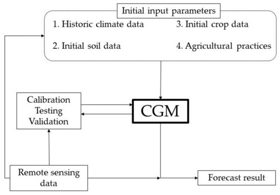
Figure 1.
Schematic representation of possible methods for integrating remote sensing data on CGM forecasts.
Ruan et al. [60] estimated the above-ground biomass (AGB), plant N content, plant N uptake, and N nutrition index based on an evolutionary algorithm-deep learning framework. Proximal sensing data collected at wheat key growth stages and corresponding meteorological data were fed into the model. They highlighted that deep neural network (DNN), random forest, and DNN-MTL (multi-task learning) all achieved promising accuracy in estimating the wheat N status. The effect of AGB accumulation and N concentration dilution across the entire growing season could be successfully captured in a single model such the one presented by Ruan et al. [60].
Clearly, the main advantage of integrating remote sensing data in CGMs is the detail of the spatial information with all the precision conferred by these data in terms of describing the real conditions of the crop. However, these data can also bring errors into the estimation, starting from the choice of method and the sensor for data collection [42,61]. Although difficulties have been pointed out for satellite platforms, mainly in terms of spatial resolution and due to the difficulty in dealing with the occurrence of clouds, launches of missions are being planned to overcome these difficulties [61]. Even so, with the existing platforms, there are results that demonstrate the pertinence of integrating remote sensing data from these platforms into CGMs. Zhuo et al. [62] demonstrated that using the LAI calculated through the MODIS platform greatly increased the estimation accuracy of the WOFOST model.
The difficulty of CGMs in generating forecasts increases as the measurements and information sources that feed the estimate increase, and which are sometimes found in different temporal and spatial resolutions [63]. A correct data assimilation process that combines process-based CGMs with agricultural data collected manually or through digital sources increases the precision and accuracy of the simulations while decreasing the reliance on extensive model calibration to a site-specific level. This assimilation reduces the uncertainties of the models, mainly regarding spatial and temporal heterogeneity [63].
3.3.2. Virtual Representation of CGMs
There is currently a great need to bring together the data integration processes to smart agriculture in a cohesive platform that guarantees the collection of relevant data and the respective analysis adapted to real problems, capable of facilitating decision making. From the moment that the manager has access to the different possible scenarios and is aware of their degree of uncertainty, they can make more appropriate and sustainable decisions. Being able to monitor the most unstable specific sites practically in real time allows for understanding their behavior and comparing them with the areas of high and low production, providing the manager with the ability to decide whether to apply N fertilizer topdressing and in what quantity [1]. Decision support systems (DSS) can manage one or more models and multiple sources of information after their calibration and validation. Even after these steps, it is important to evaluate DSSs in the field conditions for which they were designed and to compare them with the practices of farmers to measure the impact and the benefits of the implementation, such as savings of irrigation water, fertilizers, and economic profit based on growth models [33].
Due to the logical structure of process management and decision-making characteristic of a true agricultural information system, digital twins can be considered as digital technologies capable of virtually representing a complex physical system, such as agrosystem. The creation of a digital twin of the physical environment can be used to simulate the impact of events or practices carried out, anticipating and preventing eventual problems. Digital twins eliminate some restrictions on displacement and time spent on human observation, based on data collected remotely in real time, very specific from the geographic and temporal points of view and in relation to each input parameter of the CGM [1,64] (Purcell et al., 2023). Various sensors can communicate with each other and with the general platform through communication that is supported by IoT technology. While remote sensing and IoT are already well developed, adapted, and applied in the agro industry, the technology that facilitates communication between the real world and the cyber world is the cyber-physical system (CPS), which truly harnesses data and creates the digital twin. At the end of this process is the interface that allows the human user to interact and manage to integrate the system themselves. Although there is still little research on the application of this technology to the agricultural reality, it represents an excellent opportunity to achieve true digitization in an area as complex as agriculture [64].
According to Cesco et al. [1], the two main advantages of using digital twins in crop modelling are the (i) validation of management and decisions taken in the application of agricultural practices, especially when based on modelled predictions, and (ii) real-time monitoring allowed by data collected at the time, mainly by remote sensing such as satellite platforms, which inform how to adjust the N side-dresses throughout the season.
4. Conclusions
This review article describe the main movements and transformations that N undergoes in the plant−soil system, and the influence of the surrounding atmosphere of this system is also taken into account, which also ends up influencing the entire behaviour of the nutrient. It has become clear that the soil and its characteristics have the capacity to alter the entire behavior of N, making it available to be absorbed by crops, but also immobilizing or even losing it to the surrounding environment, leaving it out of reach of the plants. All of these movements can be monitored by collecting the correct data for each variable that changes them. In addition to soil variables, data on meteorological conditions, crops, and their specificities, as well as data on the agricultural practices adopted, are key to being able to calculate the movements of N in the system. These data feed tested and validated mathematical models for situations such as those we intend to predict, which end up making an estimate of the crop absorptions of N, its needs, and the possible losses of the nutrient.
It is necessary to consider that all models have gaps and uncertainties in their estimates, and it is essential to remain focused on their intended objective when using them. It must be ensured that the data that feed the model are suitable for the intended purpose. It is necessary to calibrate the model so that it is suitable for the situation in question, as well as for the subsequent validation that indicates the degree of certainty with which it manages to estimate the possible scenarios for plant growth. This review highlights statistical tests such as RMSE, NSE, and PBIAS for measuring the level of convergence of models. According to the statistical tests made by some authors, the DSSAT and DNDC models performed “good” when estimating maize N uptake.
The issue of spatial resolution of data is quite important in terms of modelling crop growth and development, as most models do not consider the spatial heterogeneity characteristic of agricultural systems. As this heterogeneity is important in the estimations of agricultural managers, it is necessary to add the ability to detail the estimates at the site-specific level to the modelling. Integrating data collected from digital sources into models makes it easier to increase the accuracy of estimates. On the one hand, it increases complexity, due to the large number of sources and data that can be incorporated, but without increasing the degree of uncertainty, as this increase in data collection does not necessarily mean an increase in errors in its collection. Remote sensing can provide timely, non-destructive spatial information and instantly improve the accuracy of model predictions. Digital data can be integrated into models right from the model calibration stage, but also through model forcing or recalibration. This assimilation reduces the uncertainties of the models, mainly regarding spatial and temporal heterogeneity.
Proper integration of digital data, such as remote sensing data, into CGMs increases the precision and accuracy of simulations, and further decreases the reliance on extensive model calibration to a site-specific level. There are different models to simulate the sensitivity of the crop yield to temperature change at a local or regional level. According to Wang et al. [65], the variation at the local scale is correlated with the global scale across the set of models. Temperature variability throughout the year has less influence on model prediction than the increase in variability between years. They added that this prediction is more compromised in places where the temperature increase is more pronounced [66]. Furthermore, this assimilation reduces the uncertainties of the models, mainly regarding spatial and temporal heterogeneity. It is this integration of detailed data at the site-specific level that ensures that model estimates are generated at the same level of spatial resolution.
When a level of great digitization of data collection from the agricultural system is reached, there are many sources that are capable of interacting with each other, but also with the manager, most of the time in real time. The advantage of this interaction allows for the creation of a virtual representation of the monitored system, commonly referred to as a digital twin, which allows managers to simulate the impact of their decisions on crop management and to avoid potential economic or environmental losses.
Author Contributions
Conceptualization, L.S.; writing—original draft preparation, L.S.; writing—review and editing, L.S.; visualization, L.A.C., F.C.L., M.P., P.D. and C.F. All authors have read and agreed to the published version of the manuscript.
Funding
The APC was funded by national funds through the Fundação para a Ciência e a Tecnologia, I.P. (Portuguese Foundation for Science and Technology) by the project UIDB/05064/2020 (VALORIZA—Research Centre for Endogenous Resource Valorization).
Data Availability Statement
Data sharing not applicable.
Acknowledgments
The authors thank the research center VALORIZA.
Conflicts of Interest
The authors declare no conflict of interest.
References
- Cesco, S.; Sambo, P.; Borin, M.; Basso, B.; Orzes, G.; Mazzetto, F. Smart agriculture and digital twins: Applications and challenges in a vision of sustainability. Eur. J. Agron. 2023, 146, 126809. [Google Scholar] [CrossRef]
- Valkama, E.; Salo, T.; Esala, M.; Turtola, E. Nitrogen balances and yields of spring cereals as affected by nitrogen fertilization in northern conditions: A meta-analysis. Agric. Ecosyst. Environ. 2013, 164, 1–13. [Google Scholar] [CrossRef]
- Plett, D.C.; Holtham, L.R.; Okamoto, M.; Garnett, T.P. Nitrate uptake and its regulation in relation to improving nitrogen use efficiency in cereals. Semin. Cell Dev. Biol. 2018, 74, 97–104. [Google Scholar] [CrossRef] [PubMed]
- Liu, K.; Harrison, M.T.; Yan, H.; Liu, D.L.; Meinke, H.; Hoogenboom, G.; Wang, B.; Peng, B.; Guan, K.; Jaegermeyr, J.; et al. Silver lining to a climate crisis in multiple prospects for alleviating crop waterlogging under future climates. Nat. Commun. 2023, 14, 765. [Google Scholar] [CrossRef] [PubMed]
- Archontoulis, S.V.; Castellano, M.J.; Licht, M.A.; Nichols, V.; Baum, M.; Huber, I.; Martinez-Feria, R.; Puntel, L.; Ordóñez, R.A.; Iqbal, J.; et al. Predicting crop yields and soil-plant nitrogen dynamics in the US Corn Belt. Crop Sci. 2020, 60, 2–721. [Google Scholar] [CrossRef]
- Kersebaum, K.C.; Lorenz, K.; Reuter, H.I.; Schwarz, J.; Wegehenkel, M.; Wendroth, O. Operational use of agro-meteorological data and GIS to derive site specific nitrogen fertilizer recommendations based on the simulation of soil and crop growth processes. Phys. Chem. Earth 2005, 30, 59–67. [Google Scholar] [CrossRef]
- Nasirahmadi, A.; Hensel, O. Toward the Next Generation of Digitalization in Agriculture Based on Digital Twin Paradigm. Sensors 2022, 22, 498. [Google Scholar] [CrossRef]
- Luce, M.S.; Whalen, J.K.; Ziadi, N.; Zebarth, B.J. Chapter two—Nitrogen Dynamics and Indices to Predict Soil Nitrogen Supply in Humid Temperate Soils. In Advances in Agronomy; Sparks, D.L., Ed.; Academic Press: Cambridge, MA, USA, 2011; Volume 112, pp. 55–102. ISBN 9780123855381. [Google Scholar] [CrossRef]
- Stockdale, E.A.; Gaunt, J.L.; Vos, J. Soil–plant nitrogen dynamics: What concepts are required? Dev. Crop Sci. 1997, 25, 201–215. [Google Scholar] [CrossRef]
- Zhang, X.; Zhang, H.; Huang, T.; Yu, C.; Feng, Y.; Tian, Y. Dynamics of soil net nitrogen mineralization and controlled effect of microbial functional genes in the restoration of cold temperate forests. Appl. Soil Ecol. 2023, 189, 104898. [Google Scholar] [CrossRef]
- Figueiredo, N.; Carranca, C.; Goufo, P.; Pereira, J.; Trindade, H.; Coutinho, J. Impact of agricultural practices, elevated temperature and atmospheric carbon dioxide concentration on nitrogen and pH dynamics in soil and floodwater during the seasonal rice growth in Portugal. Soil Tillage Res. 2015, 145, 198–207. [Google Scholar] [CrossRef]
- Akpinar, C.; Ortas, I. Impact of Different Doses of Phosphorus Fertilizer Application on Wheat Yield, Soil-Plant Nutrient Uptake and Soil Carbon and Nitrogen Dynamics. Commun. Soil Sci. Plant Anal. 2023, 54, 1537–1546. [Google Scholar] [CrossRef]
- Han, Y.; Jia, Y.; Wang, G.; Tan, Q.; Liu, X.; Chen, C. Coupling of soil carbon and nitrogen dynamics in drylands under climate change. CATENA 2023, 221, 106735. [Google Scholar] [CrossRef]
- Jia, Y.; Van Der Heijden, M.; Valzano-Held, A.Y.; Jocher, M.; Walder, F. Mycorrhizal fungi mitigate nitrogen losses of an experimental grassland by facilitating plant uptake and soil microbial immobilization. Pedosphere 2023. [Google Scholar] [CrossRef]
- Huang, J.; Deng, M.; Jia, Z.; Yang, S.; Yang, L.; Pan, S.; Chang, P.; Liu, C.; Liu, L. Influences of plant traits on the retention and redistribution of bioavailable nitrogen within the plant-soil system. Geoderma 2023, 432, 116380. [Google Scholar] [CrossRef]
- Schaeffer, S.M.; Homyak, P.M.; Boot, C.M.; Roux-Michollet, D.; Schimel, J.P. Soil carbon and nitrogen dynamics throughout the summer drought in a California annual grassland. Soil Biol. Biochem. 2017, 115, 54–62. [Google Scholar] [CrossRef]
- Delgado-Baquerizo, M.; Covelo, F.; Gallardo, A. Dissolved Organic Nitrogen in Mediterranean Ecosystems. Pedosphere 2011, 21, 309–318. [Google Scholar] [CrossRef]
- Shahnazari, A.; Ahmadi, S.H.; Laerke, P.E.; Liu, F.; Plauborg, F.; Jacobsen, S.-E.; Jensen, C.R.; Andersen, M.N. Nitrogen dynamics in the soil-plant system under deficit and partial root-zone drying irrigation strategies in potatoes. Eur. J. Agron. 2008, 28, 65–73. [Google Scholar] [CrossRef]
- Steenwerth, K.; Belina, K.M. Cover crops and cultivation: Impacts on soil N dynamics and microbiological function in a Mediterranean vineyard agroecosystem. Appl. Soil Ecol. 2008, 40, 370–380. [Google Scholar] [CrossRef]
- Villar, N.; Aranguren, M.; Castellón, A.; Besga, G.; Aizpurua, A. Soil nitrogen dynamics during an oilseed rape (Brassica napus L.) growing cycle in a humid Mediterranean climate. Sci. Rep. 2019, 9, 13864. [Google Scholar] [CrossRef]
- Kühling, I.; Mikuszies, P.; Helfrich, M.; Flessa, H.; Schlathölter, M.; Sieling, K.; Kage, H. Effects of winter cover crops from different functional groups on soil-plant nitrogen dynamics and silage maize yield. Eur. J. Agron. 2023, 148, 126878. [Google Scholar] [CrossRef]
- Lin, Z.; Price, G.W.; Burton, D.L.; Clark, O.G. Effects on soil nitrogen and plant production from land applying three types of biosolids to an agricultural field for three consecutive years. Soil Tillage Res. 2022, 223, 105458. [Google Scholar] [CrossRef]
- Ingraffia, R.; Lo Porto, A.; Ruisi, P.; Amato, G.; Giambalvo, D.; Frenda, A.S. Conventional tillage versus no-tillage: Nitrogen use efficiency component analysis of contrasting durum wheat genotypes grown in a Mediterranean environment. Field Crops Res. 2023, 296, 108904. [Google Scholar] [CrossRef]
- Fernández-Ortega, J.; Álvaro-Fuentes, J.; Cantero-Martínez, C. The use of double-cropping in combination with no-tillage and optimized nitrogen fertilization reduces soil N2O emissions under irrigation. Sci. Total Environ. 2023, 857, 159458. [Google Scholar] [CrossRef]
- Dan, X.; He, M.; Meng, L.; He, X.; Wang, X.; Chen, S.; Cai, Z.; Zhang, J.; Zhu, B.; Müller, C. Strong rhizosphere priming effects on N dynamics in soils with higher soil N supply capacity: The ‘Matthew effect’ in plant-soil systems. Soil Biol. Biochem. 2023, 178, 108949. [Google Scholar] [CrossRef]
- Sosa, L.; Panettieri, M.; Moreno, B.; Benítez, E.; Madejón, E. Compost application in an olive grove influences nitrogen dynamics under Mediterranean conditions. Appl. Soil Ecol. 2022, 175, 104462. [Google Scholar] [CrossRef]
- Ferrara, R.M.; Carozzi, M.; Decuq, C.; Loubet, B.; Finco, A.; Marzuoli, R.; Gerosa, G.; Tommasi, P.D.; Magliulo, V.; Rana, G. Ammonia, nitrous oxide, carbon dioxide, and water vapor fluxes after green manuring of faba bean under Mediterranean climate. Agric. Ecosyst. Environ. 2021, 315, 107439. [Google Scholar] [CrossRef]
- Harper, L.A.; Sharpe, R.R. Nitrogen Dynamics in Irrigated Corn: Soil-Plant Nitrogen and Atmospheric Ammonia Transport. Agron. J. 1995, 87, 669–675. [Google Scholar] [CrossRef]
- Lafuente, A.; Recio, J.; Ochoa-Hueso, R.; Gallardo, A.; Pérez-Corona, M.E.; Manrique, E.; Durán, J. Simulated nitrogen deposition influences soil greenhouse gas fluxes in a Mediterranean dryland. Sci. Total Environ. 2020, 737, 139610. [Google Scholar] [CrossRef]
- Plaza-Bonilla, D.; Álvaro-Fuentes, J.; Bareche, J.; Pareja-Sánchez, E.; Justes, É.; Cantero-Martínez, C. No-tillage reduces long-term yield-scaled soil nitrous oxide emissions in rainfed Mediterranean agroecosystems: A field and modelling approach. Agric. Ecosyst. Environ. 2018, 262, 36–47. [Google Scholar] [CrossRef]
- Sánchez-Martín, L.; Bermejo-Bermejo, V.; García-Torres, L.; Alonso, R.; Cruz, A.; Calvete-Sogo, H.; Vallejo, A. Nitrogen soil emissions and belowground plant processes in Mediterranean annual pastures are altered by ozone exposure and N-inputs. Atmos. Environ. 2017, 165, 12–22. [Google Scholar] [CrossRef]
- Dubey, R.S.; Srivastava, R.K.; Pessarakli, M. Physiological mechanisms of nitrogen absorption and assimilation in plants under stressful conditions. In Handbook of Plant and Crop Physiology; CRC Press: Boca Raton, FL, USA, 2021; pp. 579–616. [Google Scholar]
- Gallardo, M.; Elia, A.; Thompson, R.B. Decision support systems and models for aiding irrigation and nutrient management of vegetable crops. Agric. Water Manag. 2020, 240, 106209. [Google Scholar] [CrossRef]
- Pasley, H.; Brown, H.; Holzworth, D.; Whish, J.; Bell, L.; Huth, N. How to build a crop model. A review. Agron. Sustain. Dev. 2023, 43, 2. [Google Scholar] [CrossRef]
- Jiang, R.; He, W.; Zhou, W.; Hou, Y.; Yang, J.Y.; He, P. Exploring management strategies to improve maize yield and nitrogen use efficiency in northeast China using the DNDC and DSSAT models. Comput. Electron. Agric. 2019, 166, 104988. [Google Scholar] [CrossRef]
- Wajid, A.; Hussain, K.; Ilyas, A.; Habib-ur-Rahman, M.; Shakil, Q.; Hoogenboom, G. Crop Models: Important Tools in Decision Support System to Manage Wheat Production under Vulnerable Environments. Agriculture 2021, 11, 1166. [Google Scholar] [CrossRef]
- Martínez-Ruiz, A.; López-Cruz, I.L.; Ruiz-García, A.; Pineda-Pineda, J.; Prado-Hernández, J.V. HortSyst: A dynamic model to predict growth, nitrogen uptake, and transpiration of greenhouse tomatoes. Chil. J. Agric. Res. 2019, 79, 89–102. [Google Scholar] [CrossRef]
- Liu, D.; Song, C.; Fang, C.; Xin, Z.; Xi, J.; Lu, Y. A recommended nitrogen application strategy for high crop yield and low environmental pollution at a basin scale. Sci. Total Environ. 2021, 792, 148464. [Google Scholar] [CrossRef]
- Kherif, O.; Seghouani, M.; Justes, E.; Plaza-Bonilla, D.; Bouhenache, A.; Zemmouri, B.; Dokukin, P.; Latati, M. The first calibration and evaluation of the STICS soil-crop model on chickpea-based intercropping system under Mediterranean conditions. Eur. J. Agron. 2022, 133, 126449. [Google Scholar] [CrossRef]
- Puntel, L.A.; Pagani, A.; Archontoulis, S.V. Development of a nitrogen recommendation tool for corn considering static and dynamic variables. Eur. J. Agron. 2019, 105, 189–199. [Google Scholar] [CrossRef]
- Villalobos, F.J.; Delgado, A.; López-Bernal, Á.; Quemada, M. FertiliCalc: A Decision Support System for Fertilizer Management. Int. J. Plant Prod. 2020, 14, 299–308. [Google Scholar] [CrossRef]
- Kasampalis, D.A.; Alexandridis, T.K.; Deva, C.; Challinor, A.; Moshou, D.; Zalidis, G. Contribution of Remote Sensing on Crop Models: A Review. J. Imaging 2018, 4, 52. [Google Scholar] [CrossRef]
- McClelland, S.C.; Paustian, K.; Williams, S.; Schipanski, M.E. Modeling cover crop biomass production and related emissions to improve farm-scale decision-support tools. Agric. Syst. 2021, 191, 103151. [Google Scholar] [CrossRef]
- Moot, D.J.; Robertson, M.J.; Pollock, K.M. Validation of the APSIM-Lucerne model for phenological development in a cool-temperate climate. In Proceedings of the 10th Australian Agronomy Conference, Hobart, TAS, Austalia, 29 January–1 February 2001; Available online: http://www.regional.org.au/au/asa/2001/6/d/moot.htm?print=1 (accessed on 17 July 2023).
- Wilson, D.R.; Muchow, R.C.; Murgatroyd, C.J. Model analysis of temperature and solar radiation limitations to maize potential productivity in a cool climate. Field Crops Res. 1995, 43, 1–18. [Google Scholar] [CrossRef]
- Jégo, G.; Chantigny, M.; Pattey, E.; Bélanger, G.; Rochette, P.; Vanasse, A.; Goyer, C. Improved snow-cover model for multi-annual simulations with the STICS crop model under cold, humid continental climates. Agric. For. Meteorol. 2014, 195–196, 38–51. [Google Scholar] [CrossRef]
- Jägermeyr, J.; Müller, C.; Ruane, A.C.; Elliott, J.; Balkovic, J.; Castillo, O.; Faye, B.; Foster, I.; Folberth, C.; Franke, J.A.; et al. Climate impacts on global agriculture emerge earlier in new generation of climate and crop models. Nat. Food 2021, 2, 873–885. [Google Scholar] [CrossRef]
- Shahvari, N.; Khalilian, S.; Mosavi, S.H.; Mortazavi, S.A. Assessing climate change impacts on water resources and crop yield: A case study of Varamin plain basin. Iran. Environ. Monit. Assess. 2019, 191, 134. [Google Scholar] [CrossRef]
- Montenegro, S.G.; Montenegro, A.; Ragab, R. Improving agricultural water management in the semi-arid region of Brazil: Experimental and modelling study. Irrig. Sci. 2010, 28, 301–316. [Google Scholar] [CrossRef]
- Saseendran, S.A.; Singh, K.K.; Rathore, L.S.; Singh, S.V.; Sinha, S.K. Effects of Climate Change on Rice Production in the Tropical Humid Climate of Kerala, India. Clim. Chang. 2000, 44, 495–514. [Google Scholar] [CrossRef]
- Rizzo, G.; Agus, F.; Batubara, S.F.; Andrade, J.F.; Edreira, J.I.R.; Purwantomo, D.K.G.; Anasiru, R.H.; Maintang, M.O.; Ningsih, R.D.; Syahri, R.B.S.; et al. A farmer data-driven approach for prioritization of agricultural research and development: A case study for intensive crop systems in the humid tropics. Field Crops Res. 2023, 297, 108942. [Google Scholar] [CrossRef]
- Bwambale, E.; Abagale, F.K.; Anornu, G.K. Data-Driven Modelling of Soil Moisture Dynamics for Smart Irrigation Scheduling. Smart Agric. Technol. 2023, 5, 100251. [Google Scholar] [CrossRef]
- Wen, G.; Ma, B.-L.; Vanasse, A.; Caldwell, C.D.; Smith, D.L. Optimizing machine learning-based site-specific nitrogen application recommendations for canola production. Field Crops Res. 2022, 288, 108707. [Google Scholar] [CrossRef]
- Birner, R.; Daum, T.; Pray, C. Who drives the digital revolution in agriculture? A review of supply-side trends, players and challenges. Appl. Econ. Perspect. Policy 2021, 43, 1260–1285. [Google Scholar] [CrossRef]
- Divya, K.L.; Mhatre, P.H.; Venkatasalam, E.P.; Sudha, R. Crop Simulation Models as Decision-Supporting Tools for Sustainable Potato Production: A Review. Potato Res. 2021, 64, 387–419. [Google Scholar] [CrossRef]
- Gobbo, S.; De Antoni Migliorati, M.; Ferrise, R.; Morari, F.; Furlan, L.; Sartori, L. Evaluation of different crop model-based approaches for variable rate nitrogen fertilization in winter wheat. Precision Agric. 2021, 23, 1922–1948. [Google Scholar] [CrossRef]
- Diaz-Gonzalez, F.A.; Vuelvas, J.; Correa, C.A.; Vallejo, V.E.; Patino, D. Machine learning and remote sensing techniques applied to estimate soil indicators—Review. Ecol. Indic. 2022, 135, 108517. [Google Scholar] [CrossRef]
- Gautron, R.; Padrón, E.J.; Preux, P.; Bigot, J.; Maillard, O.A.; Emukpere, D. gym-DSSAT: A Crop Model Turned into a Reinforcement Learning Environment. Doctoral Dissertation, Inria Lille, Rocquencourt, France, 2022. [Google Scholar]
- Wu, J.; Tao, R.; Zhao, P.; Martin, N.F.; Hovakimyan, N. Optimizing nitrogen management with deep reinforcement learning and crop simulations. In Proceedings of the IEEE/CVF Conference on Computer Vision and Pattern Recognition, New Orleans, LA, USA, 18–24 June 2022; pp. 1712–1720. [Google Scholar]
- Ruan, G.; Schmidhalter, U.; Yuan, F.; Cammarano, D.; Liu, X.; Tian, Y.; Zhu, Y.; Cao, W.; Cao, Q. Exploring the transferability of wheat nitrogen status estimation with multisource data and Evolutionary Algorithm-Deep Learning (EA-DL) framework. Eur. J. Agron. 2023, 143, 126727. [Google Scholar] [CrossRef]
- Silva, L.; Conceição, L.A.; Lidon, F.C.; Maçãs, B. Remote Monitoring of Crop Nitrogen Nutrition to Adjust Crop Models: A Review. Agriculture 2023, 13, 835. [Google Scholar] [CrossRef]
- Zhuo, W.; Fang, S.; Gao, X.; Wang, L.; Wu, D.; Fu, S.; Wu, Q.; Huang, J. Crop yield prediction using MODIS LAI, TIGGE weather forecasts and WOFOST model: A case study for winter wheat in Hebei, China during 2009–2013. Int. J. Appl. Earth Obs. Geoinf. 2022, 106, 102668. [Google Scholar] [CrossRef]
- Kivi, M.S.; Blakely, B.; Masters, M.; Bernacchi, C.J.; Miguez, F.E.; Dokoohaki, H. Development of a data-assimilation system to forecast agricultural systems: A case study of constraining soil water and soil nitrogen dynamics in the APSIM model. Sci. Total Environ. 2022, 820, 153192. [Google Scholar] [CrossRef]
- Purcell, W.; Neubauer, T. Digital Twins in Agriculture: A State-of-the-art review. Smart Agric. Technol. 2023, 3, 100094. [Google Scholar] [CrossRef]
- Wang, X.; Zhao, C.; Müller, C.; Wang, C.; Ciais, P.; Janssens, I.; Peñuelas, J.; Asseng, S.; Li, T.; Elliott, J.; et al. Emergent constraint on crop yield response to warmer temperature from field experiments. Nat. Sustain. 2020, 3, 908–916. [Google Scholar] [CrossRef]
- Zhu, P.; Zhuang, Q.; Archontoulis, S.V.; Bernacchi, C.; Müller, C. Dissecting the nonlinear response of maize yield to high temperature stress with model-data integration. Glob. Chang. Biol. 2019, 25, 2470–2484. [Google Scholar] [CrossRef] [PubMed]
Disclaimer/Publisher’s Note: The statements, opinions and data contained in all publications are solely those of the individual author(s) and contributor(s) and not of MDPI and/or the editor(s). MDPI and/or the editor(s) disclaim responsibility for any injury to people or property resulting from any ideas, methods, instructions or products referred to in the content. |
© 2023 by the authors. Licensee MDPI, Basel, Switzerland. This article is an open access article distributed under the terms and conditions of the Creative Commons Attribution (CC BY) license (https://creativecommons.org/licenses/by/4.0/).