Article

Recognition of Tomato Leaf Diseases Based on DIMPCNET

College of Computer & Information Engineering, Central South University of Forestry and Technology, Changsha 410004, China
*
Authors to whom correspondence should be addressed.
These authors have contributed equally to this work.
Agronomy 2023, 13(7), 1812; https://doi.org/10.3390/agronomy13071812
Submission received: 28 May 2023 / Revised: 1 July 2023 / Accepted: 5 July 2023 / Published: 7 July 2023
(This article belongs to the Section Precision and Digital Agriculture)

Abstract

:
The identification of tomato leaf diseases is easily affected by complex backgrounds, small differences between different diseases, and large differences between the same diseases. Therefore, we propose a novel classification network for tomato leaf disease, the Dense Inception MobileNet-V2 parallel convolutional block attention module network (DIMPCNET). To begin, we collected a total of 1256 original images of 5 tomato leaf diseases and expanded them to 8190 using data enhancement techniques. Next, an improved bilateral filtering and threshold function (IBFTF) algorithm is designed to effectively remove noise. Then, the Dense Inception convolutional neural network module (DI) was designed to alleviate the problem of large intra-class differences and small inter-class differences. Then, a parallel convolutional block attention module (PCBAM) was added to MobileNet-V2 to reduce the impact of complex backgrounds. Finally, the experimental results show that the recognition accuracy and F1-score obtained by DIMPCNET are 94.44% and 0.9475. The loss is approximately 0.28%. This method is the most advanced and provides a new idea for the identification of crop diseases, such as tomatoes, and the development of smart agriculture.

1. Introduction

Tomatoes are vital to daily life and the vegetable trade, but their quality and quantity are susceptible to various diseases, which causes great economic losses to growers. Traditional tomato disease diagnosis relies on the long-term accumulated experience of agricultural personnel. However, this manual diagnosis is highly subjective and time-consuming. Therefore, an accurate and efficient automatic identification method for tomato diseases is urgently needed.
The diagnosis of tomato leaf disease involves two stages: image enhancement and image recognition. Researchers often use image processing techniques and machine learning methods to help identify plant leaf diseases. Physical features, such as shape, texture, and color, are used to create feature vectors, and traditional machine-learning techniques are used to identify feature vectors. However, it is difficult to extract features due to the influence of plant type, different growth stages, disease type and environment [1]. Therefore, it is necessary to use a specific image enhancement algorithm [2] before recognizing images. At present, image enhancement algorithms have been widely applied in some specific fields, such as medical research [3], remote sensing images [4] and so on. By utilizing image enhancement algorithms, some details of the image become richer, and the visuals improve [5]. There are many traditional image enhancement algorithms, but the commonly used ones include the Histogram equalization method [6], the Retinex image enhancement algorithm based on human vision [7], the unsharp mask method [8], the linear transformation method [9], etc. However, in the process of image enhancement, shadows resembling halos are prone to appear in high-contrast edge areas, known as the halo phenomenon [10]. In the 1970s, Land proposed the Retinex theory for the first time [11]. The Retinex algorithm can keep the color constant, thus eliminating the influence of the light environment on the essence of the image. In reference [12], Jobson et al. proposed a single-scale Retinex algorithm. It focuses on the brightness of the image but ignores the color. In reference [13], Hu et al. proposed the Retinex algorithm based on bilateral filtering. The algorithm takes into account the brightness of the pixel itself and the distance between the surrounding pixel positions to eliminate the interaction between high and low pixels, thereby reducing the influence of the halo phenomenon. However, this processing may result in grayscale changes in the image. In addition, the algorithm does not take fine-grained features into account in the experimental data and may not be able to accurately identify some subtle disease features. In reference [14], Zhang et al. proposed an I-Retinex algorithm that not only removes halo phenomena but also removes image noise. However, the algorithm has not studied the color image, so the image still shows a certain grayscale phenomenon. In order to further enhance image details, references [15,16] propose a contrast sharpening mask method, which can enhance high-frequency data in images, such as edge information of image targets. However, the improved image may suffer from the halo phenomenon, and the enhancement is relatively small in areas with soft light. Donoho [17] proposed de-noising methods based on frequency domain soft threshold function and hard threshold function and demonstrated the superiority of traditional de-noising methods. However, when the HF coefficient of the soft threshold approach is larger than the fixed threshold, the error is constant and the edge details are fuzzy. The hard threshold method solves the continual false trouble of the soft threshold approach [18,19]. Therefore, in view of the shortcomings of the above algorithms, we propose a Retinex image enhancement algorithm with improved bilateral filtering and an improved LF and HF coefficient threshold de-noising algorithm based on wavelet transform. The algorithm can effectively overcome the halo phenomenon, image blur, detail loss and grayscale phenomenon.
Since the invention of machine learning algorithms, they have helped identify plant diseases [20,21,22,23,24]. In the field of plant disease recognition, Wang et al. [25] used a segmentation method to extract disease plaques on apple leaves in their study and combined the color and stripe characteristics of these plaques with support vector machines (SVM) to achieve accurate disease recognition. In their study, Qin et al. [26] extracted the features of color, shape and stripe of the leaf lesions and established a recognition model of alfalfa leaf disease using naive Bayes (NBM) and linear discriminant analysis. Xie et al. [27] identified early tomato blight by studying the texture features of tomato images and achieved an accuracy rate of 88.46%. Chai et al. [28] used a combination of step-based discrimination and Bayesian discrimination to select feature parameters and a combination of principal component analysis and Fischer discrimination to construct an identification model with a recognition rate of 98.32%. For example, In the study of Zhang et al. [29], they used the SVM method to automatically distinguish three different diseases on apple leaves based on the color characteristics and histograms of apple leaf disease spots. This method can achieve 96% accuracy. Xia et al. [30] combined texture features to distinguish three types of wheat leaf disease and healthy leaves. The experimental results were better than the SVM under the same conditions. However, the machine learning algorithm also has many shortcomings. For example, before image recognition, image preprocessing and feature extraction are essential, and this process is relatively complex. But CNN can avoid the above process; it can automatically recognize the image and extract the discriminant features.
In recent years, CNN has made significant progress in computer vision. It cannot only automatically identify and extract distinguishing features but also reduce the dependence on hand motion features, resulting in better classification accuracy. For example, Wu [31] adjusted the parameters of the VGG16 and ResNet dual channel neural networks using convolution and obtained a recognition rate of maize leaf diseases of 93.33%. But this method has a low recognition rate, high image resolution, and large model parameters. Ding and Zhou [32] built a Convolutional neural network combining Transfer learning and training networks with reference to the AlexNet [33] framework. The test recognition accuracy is 96.18%, and the recognition effect is good. In their study, Guo et al. [34] proposed an improved AlexNet-based recognition model, called Multi-scale AlexNet, to accurately identify tomato diseases at different stages of onset. They effectively enhanced the ability to extract lesion features by removing AlexNet’s local response normalization layer, modifying the full connection layer, and setting up convolution nuclei of different sizes. When tested on the PlantVillage dataset, the model achieved an impressive average recognition rate of 92.7%. However, the overall recognition performance still needs to be improved. Ni et al. [35] integrated the improved Xception convolutional network and SE module into the recognition of 10 animal species, achieving high recognition accuracy. Zhang et al. [36] trained a three-channel CNN model to extract disease features and constructed a new three-channel Convolutional neural network model combining three color components. But the actual tomato leaf image has a complex background. If the color features of the diseased leaf image are only described by the three colors components R, G, and B, the color of the diseased leaf image is prone to slight changes due to the influence of the surrounding environment. Zhang et al. [37] proposed a cucumber disease recognition algorithm based on AlexNet, namely GPDCNN. This method combines extended convolution with a global pooling layer, effectively integrating contextual information, improving convergence, and optimizing the recognition rate. Six common cucumber leaf disease datasets were tested using the GPDCNN model, and the classification accuracy reached 94.65%. But the number of parameters in the network is too large, and specific methods are needed to reduce the number of parameters. Gulzar et al. [38] proposed an improved model based on MobileNetV2, TL MobileNetV2. This model achieved 99% accuracy for data from 40 different fruits. Mamat et al. [39] used the YOLOv5 model to automatically annotate images and classify the maturity of oil palm fruits, with an accuracy of 98.7%. Aggarwal et al. [40] proposed a stacked ensemble method to obtain better F1 scores by combining three pre-trained models: VGG16, ResNet152, and DenseNet 169. The results show that assembling different weak Convolutional neural networks can produce better predictions than a single model. Research with CNN and Transfer learning as the core classifies 14 common seeds [41]. They claim that they have achieved great success, which indicates the progressiveness of deep learning technology. Chen et al. [42] proposed a dual-channel residual attention network model, B-ARNet, to classify 8616 tomato leaf disease images, but the overall accuracy can only reach 89%. Alom [33] et al. proposed an improved network architecture based on CNN, LeNet, to identify tomato leaf diseases. To some extent, it has reduced computational resources. The model achieved an average accuracy of 94–95%. However, due to the limited training data, this model is not suitable for tomato leaf recognition in complex backgrounds. Zhang et al. [43] proposed M-AORANet to extract and recover fine multi-scale features by locating lesion sites on tomato leaves, solving the problem of identifying similarities between tomato leaf diseases. The experimental results on 7493 images show that the recognition accuracy of M-AORANet reaches 96.47%. Sun et al. [44] optimized the AlexNet network model by reducing the size of convolutional kernels and the number of parameters. Gibran et al. [45] improved the CNN network model, optimized the dataset through data augmentation, and adjusted and optimized the hyperparameters of the model, achieving an accuracy of 94%. Cai et al. [46] proposed the DWOAM DRNet network for grape disease leaf recognition, which utilizes multiple branch blocks to construct residual connection strategies, enriches the feature space, and improves the network’s response to features. To some extent, it solves the problem of high disease similarity that makes it difficult for models to distinguish. Its recognition accuracy reaches 93.26%. This method provides us with ideas.
Combined with previous studies, this study needs to consider the following issues: (1) External environmental factors can easily affect the quality of images. When the original dataset of tomato leaves is directly fed into the network, the CNN structure automatically learns features from the training set. Unfortunately, due to the presence of noise and other factors, the original image may be distorted, leading to inaccurate feature extraction and ultimately resulting in poor network recognition. (2) Tomato leaf diseases often exhibit similar characteristics within certain categories. Additionally, the initial and final images of a disease can vary significantly. The initial lesion area is typically narrow, and the symptoms may be unclear, making accurate identification challenging. To address this, it becomes necessary to extract more detailed features from the network layer in order to capture the multi-dimensional and multi-scale aspects of the disease. Furthermore, the background environment in which diseased leaves are collected in natural scenes is highly complex. When extracting features, the network model must effectively filter out the background environment features and focus on extracting as many relevant features as possible. This helps to minimize the interference of the complex background on the accuracy of disease recognition. Given these challenges, designing an optimal CNN structure for the detection of tomato leaf diseases becomes an arduous task that requires careful consideration. The innovations of this paper are as follows:
  • In order to optimize the performance of disease features, an improved IBFTF image enhancement algorithm is proposed, in which wavelet transform is used to combine image enhancement and de-noising. Firstly, the noise image is decomposed by wavelet, obtaining the low frequency (LF) and high frequency (HF) coefficients. The HF coefficients were denoised using an enhanced threshold function method, while the LF coefficients were denoised using an improved bilateral filtering Retinex image enhancing algorithm. Then, the rebuilt image is obtained by inverse wavelet transform. Finally, to boost the comparison of the rebuilt image, linear segmentation processing is utilized. In comparison to existing algorithms, this approach can remove the halo effect, image blur, detail loss, and grayscale phenomenon from the image and effectively remove noise;
  • Aiming at the problems of complex background of natural scene images, small differences in disease classification, and difficult model recognition, we propose a method of tomato leaf disease recognition based on DIMPCNET. The method is described below.
    • A new depth Convolutional neural network module DI is proposed, which uses depth separable convolution to construct the first two layers of convolution, reducing the number of parameters and avoiding overfitting of the model. We introduce the initial structure into the model to enhance the extraction performance of multi-scale pathological features and adopt a dense connection strategy for the four initial structures to improve the response of the network to features and alleviate gradient disappearance. We have made progress in extracting the depth characteristics of the disease area, reducing the similarity difference between different disease leaves, solving the problem of indistinguishable caused by highly similar disease leaves, and enhancing the overall performance of the model;
    • A new hybrid attention module, PCBAM, is proposed. It connects channel attention and spatial attention in parallel, which solves the interference problem caused by serial connection, effectively improves the feature extraction ability of the model, weakens unnecessary features, and reduces the influence of complex background on the discrimination results;
  • The method proposed in this paper achieved recognition accuracy of 94.44% and an F1 value of 0.9475 for the identification of five types of tomato leaf diseases. It is effective to identify tomato leaf diseases with complex backgrounds and high similarity between classes. This allows agricultural experts and scholars to better apply this technology to the prevention and control of tomato diseases so as to effectively alleviate food production problems to a certain extent.
The structure of this article is summarized as follows: Section 2 introduces the materials and methods for identifying tomato leaf disease. Then, Section 3 introduces tomato leaf disease identification based on the DIMPCNET model. Section 4 introduces experimental results and analysis to verify the superiority of the network. Finally, we summarized the entire article and proposed future prospects.

2. Materials and Methods

2.1. Data Acquisition

Data collection is a vital component of the study. Since there is no appropriate data set to diagnose illnesses on tomato leaves, it took us a long time to collect the dataset. It contains five categories of tomato leaves, including early blight, leaf mold, gray mold, gray leaf spot, and healthy leaf. The dataset was obtained from a total of 5 shots taken at the demonstration site of the Hunan Provincial Vegetable Research Institute from June to August 2022. All photographs were captured with a Sony camera with a resolution of 4460 × 3740 in natural sunlight. One thousand two hundred fifty-six images of tomato leaves were collected by the camera, including 312 images of early blight tomato leaves, 314 images of leaf mold tomato leaves, 356 images of gray mold tomato leaves, 323 images of gray leaf spot tomato leaves, and 333 healthy leaf images, all of them are saved in jpg format. Figure 1 depicts some representative images. We fully considered the diversity of the samples and, therefore, took photos under different backgrounds, weather conditions, and different stages of disease development. Its purpose is to provide comprehensive and accurate disease image samples.
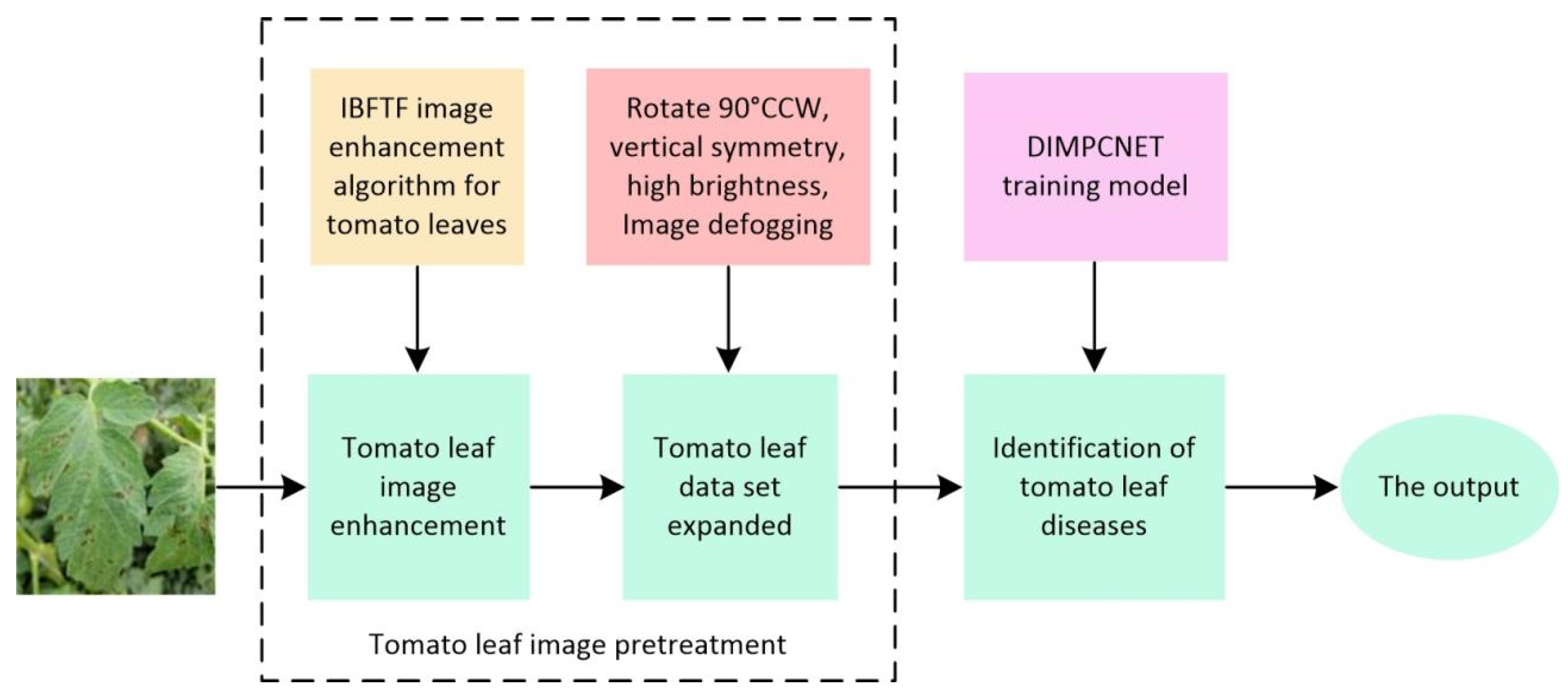
Tomato leaf disease recognition involves fine-grained image classification, where the focus is on learning discriminative features and detecting subtle differences between visually similar samples [47]. To enhance the classification accuracy of tomato leaf disease recognition, further research is required. This is particularly important due to the challenges posed by the natural environment and the interference of environmental conditions and noise on image data. In this regard, the proposed IBFTF image enhancement algorithm plays a significant role. To prevent model overfitting, the dataset was augmented through techniques such as 90-degree rotation, left-right symmetry, increased brightness, and image atomization. Finally, we fed the preprocessed dataset into the DIMPCNET network model for training in order to recognize tomato leaf disease images and consider disease features. The working principle of this study is shown in Figure 2.

2.2. Image Augmentation

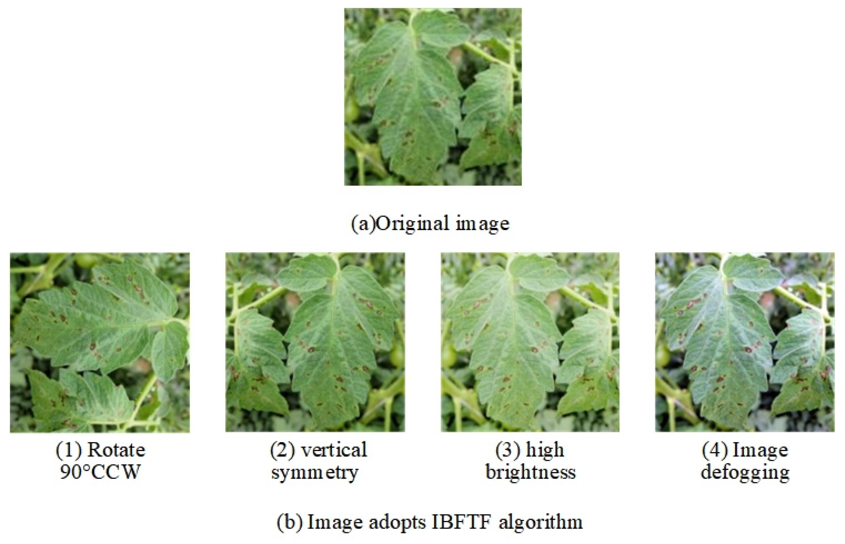
Data augmentation offers several advantages, with the most significant being its ability to mitigate the overfitting problem encountered by convolutional neural networks during training. When the available dataset is limited, data augmentation techniques become particularly valuable. By expanding the original image through various operations, such as counterclockwise rotation, left-right symmetric transformation, brightness adjustment, and de-fogging, the aim is to prevent overfitting and enhance the model’s generalization capabilities. Data augmentation facilitates the generation of additional images, enabling the model to learn from a more diverse range of patterns during training. This not only helps in avoiding overfitting but also strengthens the model’s ability to handle challenging scenarios by improving its resistance to interference. Figure 3 illustrates the process of image generation.
After the image enhancement process, a dataset of diseased tomato leaf images was obtained, which included 1560 photos of early blight, 1570 photos of leaf mold, 1780 photos of gray mold, 1615 photos of grey leaf spot, and 1665 photos of healthy tomato leaves. Then, we resized all images in the dataset to 224 × 224. Finally, the dataset was separated into three sections: the training set, the validation set, and the test set, in a 6:2:2 ratio. The specifications of the data set are depicted in Table 1.

2.3. Tomato Leaf Image Enhancement Based on IBFTF

The image of diseased tomato leaves often suffers from low contrast and uneven brightness due to external environmental factors. While enhancing the contrast can improve visibility, it may also amplify image noise, blur the edges, and result in unclear details, ultimately affecting the quality of tomato leaf disease recognition. To address this issue, an image enhancement algorithm based on the IBFTF algorithm was proposed. This algorithm enriches image details and improves visual effects, which is crucial for subsequent recognition research.
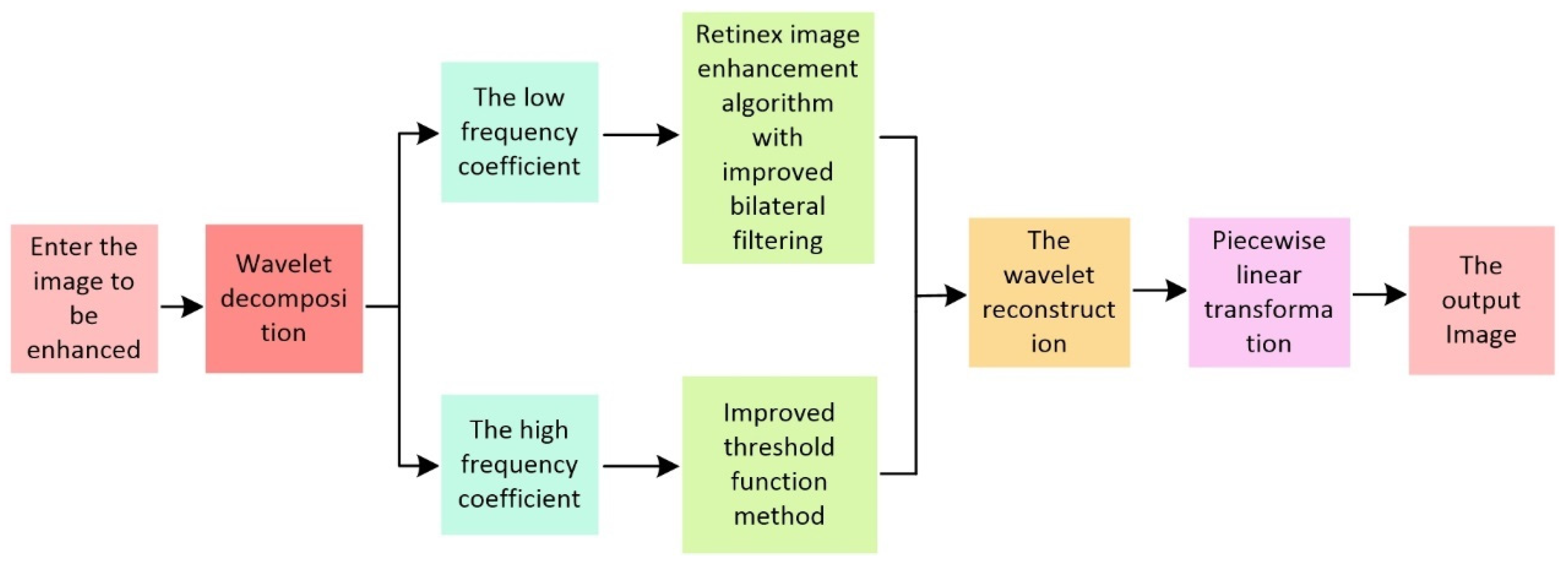
To effectively address the mentioned issues, we use the wavelet transform method to combine the idea of image enhancement and image de-noising. Firstly, the LF and HF coefficients of the noisy image are acquired by decomposition with a wavelet. The LF coefficients are strengthened by the Retinex image enhancement algorithm with improved bilateral filtering, and the HF coefficients are de-noised by an improved threshold function method. Then, rebuilt visual is created by an inverse wavelet transform on the processed LF and HF coefficients. Finally, to raise the contrast of the reconstructed image, it employs the piecewise linear transformation technique, which effectively solves the above-targeted problems. The algorithm in this work has the following exact actions:
  • The noise image is decomposed using wavelets, and both the low and HF coefficients are calculated;
  • The LF coefficients are handled by the enhanced bilateral filtering Retinex image-enhancing method;
  • The method of improved threshold function is designed to handle the HF coefficient;
  • The reconstructed image is obtained by wavelet reconstruction of both LF and HF coefficients;
  • The reconstructed image is processed by a piecewise linear transformation, and the enhanced image is obtained.
Algorithm 1 depicts the algorithm framework depicted in the above steps. Figure 4 depicts the flow chart of the IBFTF image enhancement method.
Algorithm 1: IBFTF image enhancement
Input: Image S ( x , y )
1. Decompose the noisy image into LF W Ø and HF W φ i coefficients
2. The image is launched R x , y
3.  W Ø uses enhanced bilateral filtering I D ( i , j ) processing
4.  W ( i , j , k , l ) , W ( i , j , k , l ) sets the filtering window parameter P , and the original bilateral filtering window size is 2 P + 1
5. The enhanced threshold function ω J , K is used to estimate the HF wavelet coefficient in three parts
6. Process W Ø using f ( i , j ) three-segment piecewise linear transformation
7.  W Ø and W φ i are reconstructed using 2D discrete wavelet f ( x , y )
8. Output reconstructed image

2.3.1. Wavelet Decomposition and Reconstruction

In this paper, the wavelet transformation divides the noise image into LF and HF coefficients. The LF coefficients primarily contain global image information, including contour information, whereas the HF coefficient primarily contains local image information. The following is the formula for two-dimensional (2D) discrete wavelet decomposition:
W Ø j 0 , m , n = 1 M N x = 0 M 1 y = 0 N 1 f ( x , y ) ϕ j 0 , m , n ( x , y ) ,
W φ i ( j , m , n ) = 1 M N x = 0 M 1 y = 0 N 1 f ( x , y ) φ j , m , n i ( x , y ) ,
i = H , V , D
where W Ø ( j 0 , m , n ) is decomposed LF coefficients, and W φ i ( j , m , n ) is decomposed HF coefficient; H, V, D, j 0 is an arbitrary starting scale, usually they are set to zero; F (x, y) is a discrete function, the parameters x and y are discontinuous; m and n are the relative offset from (x, y), M and N represent that the image is composed of M and N pixels, ϕ j 0 , m , n ( x , y ) is a two-dimensional scale function, which is the horizontal, vertical, and diagonal wavelet function of i.
Combining W Ø ( j 0 , m , n ) and W φ i ( j , m , n ) , LF and HF coefficients are handled using the Retinex image enhancement technique with modified bilateral filtering and threshold function method. The images were reconstructed by discrete wavelet inversion [48]. The inverse one-dimensional (1D) discrete wavelet transform is first applied to each column of the decomposition result. Then each row of the transformed data is transformed by the inverse one-dimensional discrete wavelet transform to obtain the reconstructed image. The following is the wavelet reconstruction formula:
f ( x , y ) = 1 M N m n W Ø j 0 , m , n Ø j 0 , m , n ( x , y ) + 1 M N i = H , V , D j = j 0 m n W φ i ( j , m , n ) φ j , m , n i ( x , y )

2.3.2. Improved Retinex Algorithm for Bilateral Filtering

The image seen by humans, according to Retinex theory, is divided into two sections: the illuminative image and the reflective image,
S ( x , y ) = R ( x , y ) × L ( x , y )
where S ( x , y ) is the actual image, R ( x , y ) is the reflected image, and L ( x , y ) is the illuminated image, which reflects the dynamic spectrum that the image can reach, including conditions such as illumination intensity and environment, while the reflected image responds to information such as image vein and contour [49]. The Retinex algorithm obtains the reflection image that reflects the essence of the image by removing lighting components from the original image and transforming the logarithmic domain. Meanwhile, a light adjustment parameter k(k ∈ (0,1)) is added to eliminate the abnormal phenomenon of the image. The following is the reflected image formula:
R ( x , y ) = log a S ( x , y ) k log a S ( x , y ) F ( x , y )
The illumination image L ( x , y ) is created by convoluting the original image with the Gaussian kernel function, where K is the brightness modification parameter and F ( x , y ) is the Gaussian kernel function.
The Retinex algorithm based on bilateral filtering, which considers the Euclidean distance of pixel values and the radiation differences within the pixel range, improves the halo phenomenon generated by the single-scale algorithm. This is the formula for bilateral filtering:
I D ( i , j ) = k , l I ( k , l ) W ( i , j , k , l ) k , l W ( i , j , k , l )
I D ( i , j ) is the output image, I ( k , l ) is the original image, and W ( i , j , k , l ) is the kernel function of the spatial domain and pixel range domain. In a flat area with a small change in image pixel value, bilateral filtering is mainly used in the area of space, which is comparable to Gaussian filtering. The spatial domain and pixel value domain are considered simultaneously in the edge region where the pixel value changes greatly, which can keep the image’s edge information while effectively avoiding the halo phenomenon caused by the large difference in image brightness at the edge. The bilateral filtering formula is as follows:
W ( i , j , k , l ) = exp ( i k ) 2 + ( j l ) 2 2 σ d 2 I ( i , j ) I ( k , l ) 2 2 σ r 2
In this paper, we advise utilizing the Retinex image enhancement method with optimized bilateral filtering and improving the spatial domain of pixels in the bilateral filtering kernel function. Here is the optimized bilateral filtration formula:
W ( i , j , k , l ) = 1 ( i k ) 2 + ( j l ) 2 p exp I ( i , j ) I ( k , l ) 2 σ r 2 ( i k ) 2 + ( j l ) 2 p
where σ d is the distance difference scale parameter, σ r is the brightness difference scale parameter, and p is the filter window parameter.
In the spatial domain, the filtering window parameter p is set. The size of the filtering window of the original bilateral filtering is 2p + 1, and the filtering window of the improved bilateral filtering is a circular area with the filtering center pixel as the center and the filtering parameter p as the radius. When the pixel distance between the filter neighborhood and the filter center is less than the filter window parameter, the pixel is positioned within the radius, then both the spatial domain and the value domain of the pixel are valid so that the image edge information is maintained while smoothing the noise. When their pixel distance exceeds the filtering window parameter, it is considered that the pixel is far away from the center pixel, and then the pixel is not processed to eliminate the effect of the pixel on the image edge. The reflected image obtained by the improved bilateral filtering algorithm not only keeps the edge details effectively but also removes the halo phenomenon better.

2.3.3. Wavelet HF Coefficient Processing

This study suggests an enhanced threshold function with the following formula:
ω J , K = sgn ω j , k ω j , k 0.5 λ , ω j , k λ sgn ω j , k λ / ( λ 0.6 λ ) ω j , k 0.5 λ 0.6 λ ω j , k < λ 0 , ω j , k < 0.6 λ
where ω J , K is the calculated HF coefficient after threshold analysis, ω j , k is the HF coefficient obtained by decomposing, λ represents the threshold, and the improved threshold function takes λ and 0.6 λ as the cut-off point to estimate the HF wavelet coefficient in three parts. When the HF coefficient is greater than the fixed threshold, the estimated HF coefficient is half of the difference between the HF coefficient and the fixed threshold, and the improved threshold function reduces the constant error compared to the soft threshold function. When the HF coefficient is between 0.6 λ and λ , Equation (14) can be used to effectively improve the HF coefficient. When the HF coefficient is less than 0.6 times the preset threshold, the calculated HF coefficient is set to 0. Compared with the traditional threshold function, the algorithm is divided into three parts to increase the estimated HF coefficient, distinguish the noise component more clearly, avoid the oscillation phenomenon effectively, and decrease the constant deviation of the threshold function.
In this study, after the wavelet decomposition, the improved bilateral Retinex filtering method is used to enhance the LF coefficient image, and the improved threshold function is used to process the decomposed HF coefficient. Then the inverse wavelet transform is used to reconstruct the image.

2.3.4. Contrast Enhancement

After using the Retinex algorithm to process the LF coefficients and the threshold function is improved to de-noise, the reconstructed image has a grey phenomenon. The approach of three-segment piecewise linear conversion is utilized to increase image contrast in this paper; the formula is given below for the three-segment piecewise linear transformation:
f ( i , j ) = k 1 × d ( i , j ) , 0 d ( i , j ) < a b + k 2 × d ( i , j ) , a d ( i , j ) c d + k 3 × d ( i , j ) , c < d ( i , j ) 255
f ( i , j ) represents the final image after boosting, d ( i , j ) is the input image, k 1 , k 2 , and k 3 are the slopes of the three-segment transformation, and their expressions are as follows:
k 1 = a b k 2 = d b c a k 2 = 255 d 255 c
(a, b) and (c, d) are the points on the piecewise function where the slope changes and the piecewise linear transformation raises the image contrast.
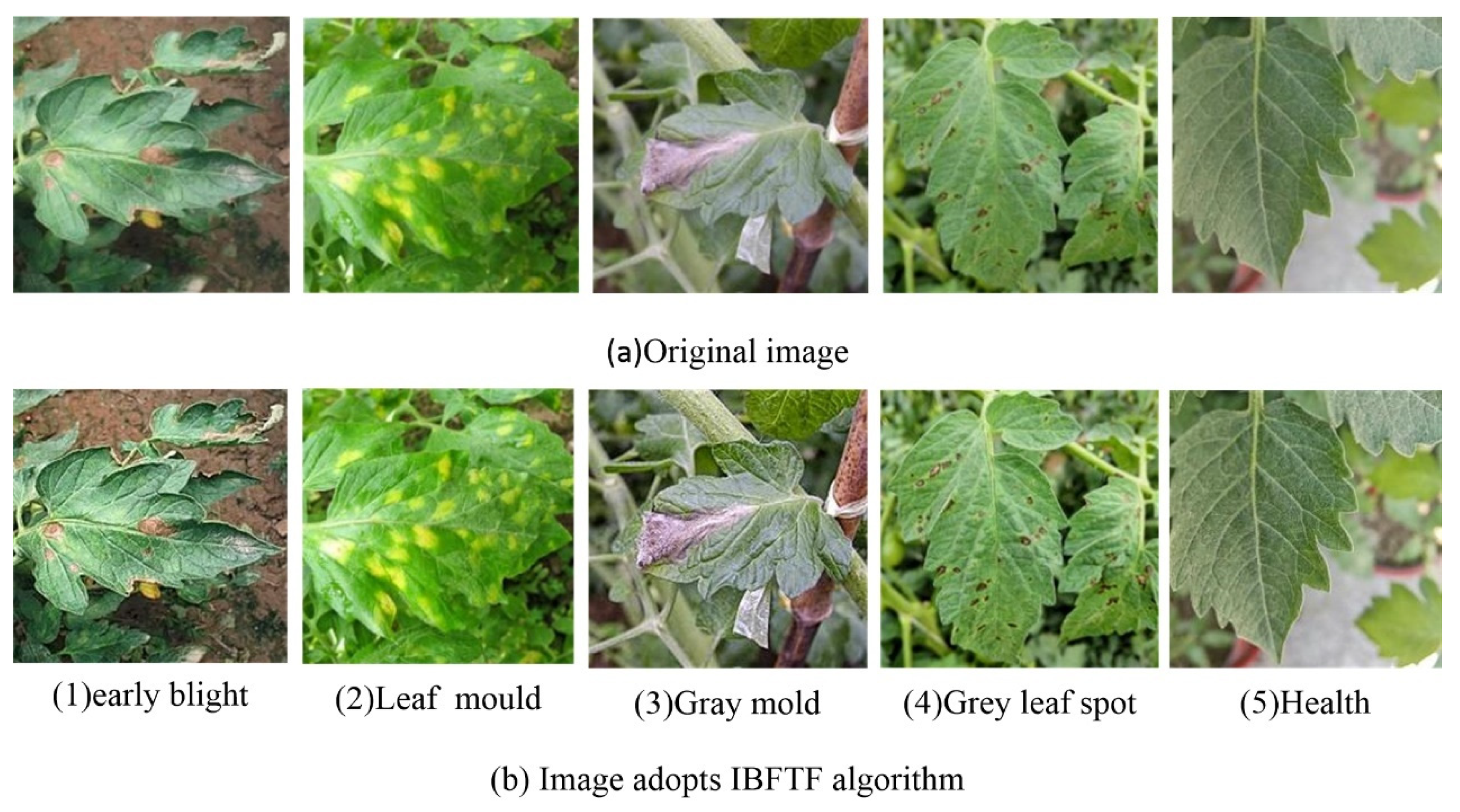
Figure 5 shows several examples of enhanced images. Figure 5a is the original image, and Figure 5b is the image enhanced by the IBFTF algorithm.

3. Tomato Leaf Disease Recognition Based on DIMPCNET Model

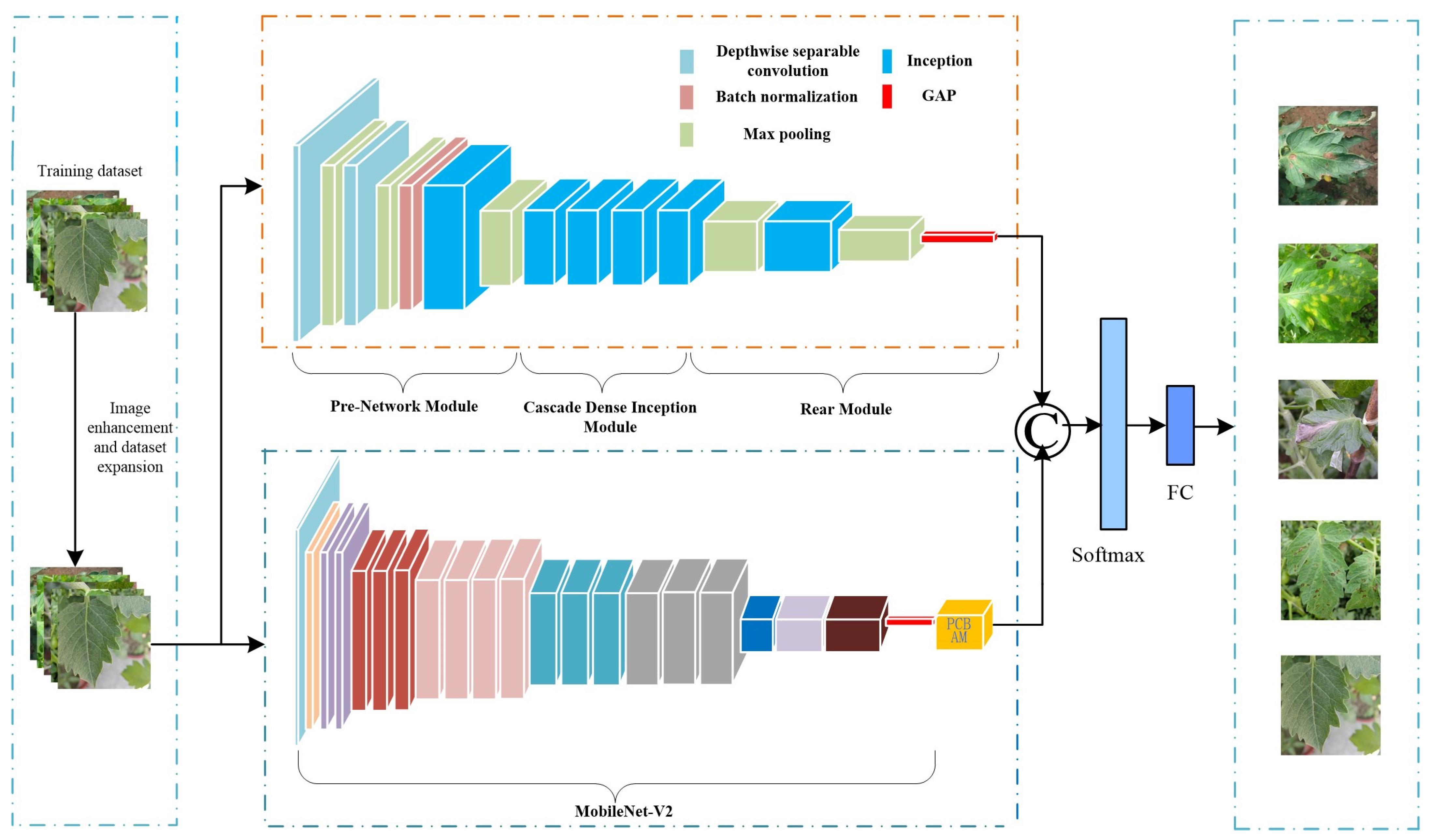
This article proposes a DIMPCNET model to help identify tomato leaf diseases. Compared with traditional CNN, it is special in that it adopts a dual-branch parallel structure. Each branch uses the basic Convolutional neural network as the feature extractor. The two branches can be symmetric or asymmetric structures and then uses bilinear pooling to achieve feature fusion. The first step is to replace the four dense blocks in DenseNet [50] with Inception structures and implement a dense connection strategy for the four Inception modules to extract multi-dimensional and multi-scale information about diseased leaves. Among them, the Inception structure contains convolutional kernels of different sizes. Therefore, the multi-channel parallel structure of Inception can extract features from both the overall information within the global range and the detailed information within local regions, such as color and texture features [51]. By adopting this approach, the problem of small inter-class variance caused by similar characteristics of different diseased leaves and large intra-class variance caused by leaf diseases at different stages can be alleviated. In a second way, PCBAM was introduced into the MPC module to mitigate the effect of complex backgrounds on recognition and remove unnecessary, redundant information, such as background, and increase focus on the disease characteristics. Figure 6 shows the overall structure of DIMPCNET. Then, the construction of DI and the principle of the MPC module are introduced in detail.
DIMPCNET is primarily utilized for fine-grained image categorization tasks. What sets DIMPCNET apart from conventional CNNs is its utilization of a two-branch parallel structure. Each branch employs basic convolutional neural networks as feature extractors, and these branches can have either symmetric or asymmetric structures. Feature fusion is achieved through the application of bilinear pooling. The underlying concept behind the design of DIMPCNET is to mitigate the negative impact of complex background environments and the similarity of disease spots on disease identification. This is accomplished by extracting multi-dimensional and multi-scale features from diseased leaves. In a two-branch arrangement, the weights of each branch are not shared. The key aspect of this network structure is the utilization of the two-branch network to derive more efficient features of disease spots. The retrieved features differ based on the varying structures of each branch network. Figure 6 depicts the DIMPCNET network structure, where © denotes Concat connection, FC stands for full connection layer, and Softmax represents an activation function.
DIMPCNET network structure can be divided into three parts: DI, the MPC module, and the final feature fusion part. The input is a disease image of size 3 × 224 × 224, and the features of the image are extracted by DI and MPC modules, respectively. Both branches adopt self-built CNN as the basic network and adjust each branch network according to the different functions of the two channels in DIMPCNET. The DI enhances the performance of multi-dimensional feature extraction by using Inception architecture [52,53,54,55]. In addition, a dense join strategy is introduced to promote feature reusing and improve the dissemination of features. Finally, we built and trained a new CNN-based model from scratch, namely DI, to derive multi-dimensional and multi-scale characteristics so as to alleviate the problem of a short gap between classes and a wide gap within classes. The MPC module is based on Mobile-NetV2 by adding a PCBAM attention mechanism, which links simultaneous channel and geographic focus so that the model emphasizes the important portions of the image and ignores the complex background and other useless information. Finally, the DI and the MPC module pool the extracted features globally. In addition to reducing the model parameters, the Concat method is adopted for feature fusion. Finally, the Softmax function is employed to identify tomato leaf diseases.

3.1. DI Module

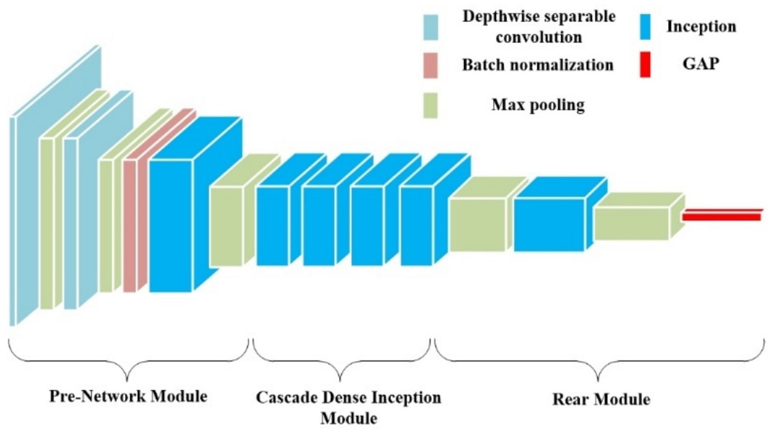
Figure 7 shows the DI. A new depth Convolutional neural network module DI is proposed, which uses depth separable convolution to construct the first two layers of convolution, reducing the number of parameters and avoiding overfitting of the model. The module is divided into three parts: the pre-network module is the first part. Its two depth-separable convolutional layers are filtered by 64 convolutional kernels, and a max-pooling layer is added between the two depth-separable convolutional layers, followed by a maximum pooling layer and a regularization layer, and a starting structure and a max-pooling layer. The second module consists of four consecutive Inception structures, which are densely connected. Due to the densely connected strategy, the obtained feature maps are more efficient, multi-dimensional features are better integrated into the Inception structures, and the model is better at identifying tomato leaf disease. The last module consists of two maximum pooling layers, an Inception structure, and a global average pooling (GAP) layer.

3.1.1. Depth-Separable Convolutional Layer

Because there are few images in the tomato leaf disease dataset and over-fitting is common during the training of large-size models, reducing the number of parameters has a positive impact on model generalization performance. Furthermore, the fewer model parameters that are used, the faster the training efficiency is and the less computational power that is needed. Deep convolution and point convolution combine to form the deep divisible product, and experimental results show that it has fewer parameters than conventional convolution (Howard et al., 2017) [56]. In depth-separable convolution, each input channel is deeply convolved using a single filter, and then outputs are combined by a 1 by 1 convolution operation by point convolution. This decomposition method significantly reduces the scale of the model and its use of computational resources but does not reduce the model accuracy rate.

3.1.2. Cascading Dense Inception Modules

The severity of spots can vary among different types of tomato leaf diseases, and even within the same type of diseased leaves, the size of the spots can vary across different periods. However, the model’s ability to extract features at different scales greatly impacts the final accuracy of recognition. To capture features of varying sizes, a densely connected Inception module is incorporated into the model, consisting of four consecutive Inception structures. In order to extract fine-grained lesion features, small-size convolution kernels are employed, while large-size convolution kernels are used to extract features of larger lesions. This approach is inspired by the Inception structure of GoogleNet. The Inception structures include parallel branches with convolution layers of different sizes, allowing each branch to focus on a specific feature. It improves the functionality of multi-scale feature extraction while also widening the network. In addition, based on the asymmetric decomposition method [57], asymmetric convolution is adopted to increase the efficiency of extracting features, and the computational cost is also reduced.
In general, the time complexity of CNN models is evaluated by floating-point arithmetic. One way to express the temporal complexity of a single convolution layer is as follows:
  Time O M 2 K 2 C in C out
The edge lengths of the output feature map and the convolution kernel are denoted by M and K, respectively; the number of channels in the input feature map is denoted by Cin, and the number of channels in the output feature map is denoted by Cout.
Numerous convolution layers make up the Inception architecture, and the temporal complexity of this structure is defined as the sum of all convolution layer operational times:
  Time O i = 1 D M i 2 P i Q i C ( i , in ) C ( i , o u t )
Pi stands for the distance of the convolution kernel, Qi for the width of the convolution kernel, and D for the number of convolution layers in the Inception structure (Qi is not equal to Pi if using asymmetric convolution).
When creating a feature diagram, transferring small-scale features in tomato leaf diseases to deeper levels of the model is difficult. The removal of this feature has a significant impact on the accuracy rate of the model. In DenseNet, to further enhance the information flow between layers, a dense connectivity technique is suggested. Layer l obtains the attribute mapping of the preceding layers, as shown in the formula:
x = H α x 0 , x 1 , x α 1
[ x 0 , x 1 , , x α 1 ] indicates the mapping connection of the previous layer.
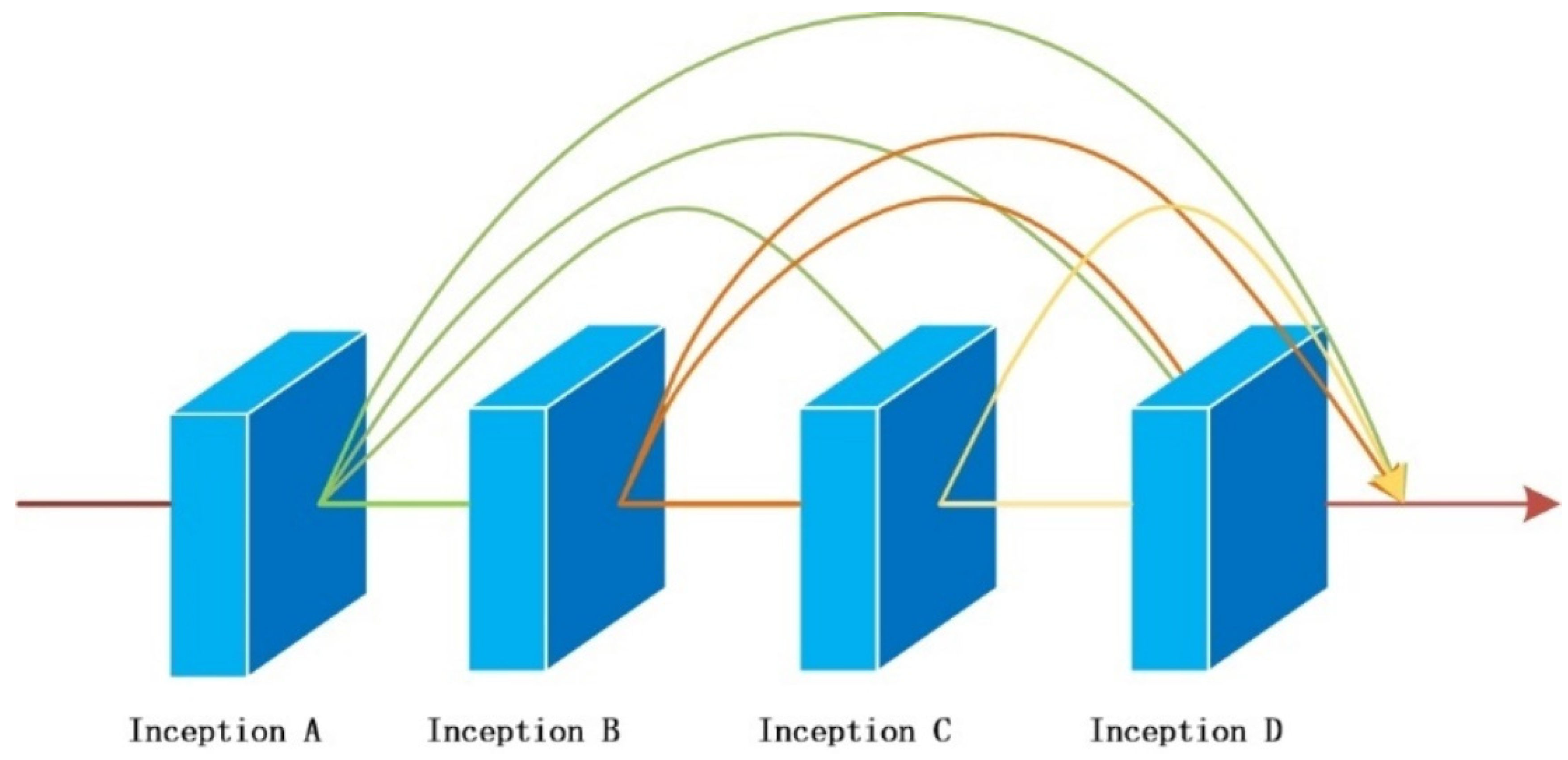
As shown in Figure 8, the four Inception modules use the dense connectivity strategy. As a result, the feature map of all previous layers in this module is taken as the input of this layer, and its own feature map is taken as the input of all subsequent layers. The recognition ability of the model can be significantly improved by using the dense connection strategy because it strengthens the propagation of features and encourages the reuse of features, which can successfully stop the occurrence of an overfitting phenomenon. Finally, ResNet with residual structure was compared; this method greatly reduces the parameter and model storage costs.

3.2. The MPC Module

In order to alleviate the problem of the influence of complex background on the recognition effect and to reduce the size and number of parameters of the model, the PCBAM module is embedded in the lightweight mobile neural network MobileNet-V2 to improve the recognition effect of fine-grained tasks, so as to improve the overall recognition accuracy of the model.
Soft attention and strong attention are two primary forms of attention mechanisms used in convolutional neural networks. Soft attention primarily focuses on specific areas or channels with a relatively strong level of certainty. It is generated through the network after the learning process is completed. Soft attention is differentiable, which distinguishes it from non-differentiable strong attention. Differentiable attention can be computed by neural networks using gradients, allowing for forward propagation and backward feedback to learn the attention weights. However, this type of soft attention is computationally expensive, as it involves a large number of parameters. The activation functions used to achieve attention are independent of each other. Soft attention can select multiple targets simultaneously, but in practical applications, it is often desirable to be more selective and focus on only one element of the scene. Soft attention can also adjust the input size to further enhance performance. In the domain of image research, the hard attention mechanism is employed to select the relevant focus area as input, effectively emphasizing the target object by eliminating irrelevant background data. This mechanism directly restricts the input, but its applicability is limited in the field of timing forecasting. In time sequences, the relevance of input varies, and each input subsequence contains specific information that is distributed across different positions throughout the sequence and cannot be easily discarded. Moreover, maximizing the hard learning algorithm requires complex reward learning, which is difficult to achieve and lacks generality. On the other hand, the soft attention mechanism utilizes neural network weights to assign importance to global input features in space or channels, achieving the goal of focusing on a specific spatial area or channel. This method is differentiable, allowing for reverse computation and enabling the adoption of an end-to-end learning approach to directly train the attention network. This paper primarily employs soft attention. Soft attention can be categorized into three domains: channel domain, mixed domain, and spatial domain. Among these, the spatial and channel domains are the aspects of soft attention explored in this study.
When performing classification tasks, Spatial attention [58] can force neural nets to focus more on the most crucial pixel areas while neglecting unimportant parts. Relationships of feature maps are taken into account via the attention process known as Channel attention [59]. The hybrid domain is a combination of these two different kinds of attention. CBAM combines geographical and channel attention in the convolution module to achieve a progressive attention architecture from channel to space, which can be embedded into the convolution operation and easily transplanted. In the CBAM [60] module, the feature map F is input first, and the result is F 1 after the channel attention weighting. After spatial attention weighting, the “cascade connection”-style output feature map F 2 , whose formula is obtained, is acquired:
F 1 = M c ( F ) F F 2 = M s F 1 F 1
where M C F 1 is the channel attention output weight of F and M s F 1 is the spatial attention output weight of F 1 , and ⨂—weighted multiplication notation operation of the feature map.
In fact, either channel attention is enabled first and then spatial attention (CBAM), or spatial attention is enabled first and then channel attention (reverse CBAM). The weights at the bottom are generated from the feature map at the top. In this process, the attention that comes first “embellishes” the original input feature map. That is, what the attention mechanism at the bottom learns is the “modified” feature map, which affects the features learned by the attention module at the bottom to a certain extent. Especially in fine-grained classification tasks, such interference caused by “serial connection” will make the influence of the attention module unsteady [61]; therefore, it is hard to guarantee accuracy improvement.
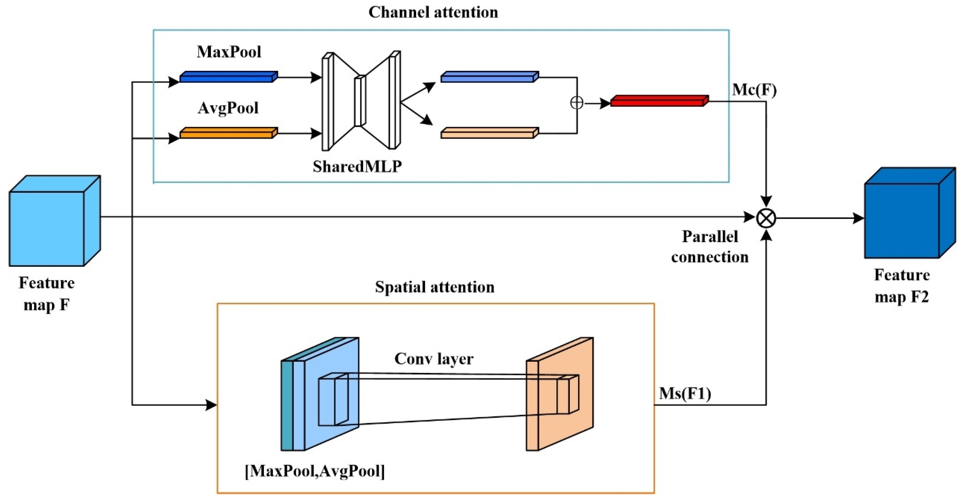
Therefore, to address this issue, this paper improves the serial attention module of CBAM by changing the original “Cascade connection” into a “parallel connection” so that the initial input feature map can be learned by the two attention modules, negating the requirement for them to focus on spatial attention and channel attention order. This results in a parallel connected CBAM. Prior to combining the weights with F to create the output feature map F 2 , PCBAM first collects the matching weights from F using both channel and spatial attention, whose formula for the procedure is F 2 = M c ( F ) M s F F ( 2 ) . In the formula, M s F F passes the output weight of spatial attention, and Figure 9 depicts the general structure of PCBAM.
MobileNet-v2 is a lightweight model. However, when the model is pre-trained using ImageNet in the experiment, if each residual inversion module of Mobilenet-V2 has an attention mechanism, the initial settings for the trained model will be seriously damaged during training, and the scale of the model will also become several times of the original one. At that time, the lightweight meaning of Mobilenet-V2 had been lost. Therefore, we carried out comparison experiments; the attention module was embedded after the last convolution of Mobilenet-V2, and the batch normalization layer (BN) after convolving was deleted so as to lessen parameter disruption and guarantee training robustness.

4. Experimental Outcomes and Analysis

4.1. Environment and Setup for Experiments

The self-built data set included five categories of tomato leaves, including early blight, leaf mold, gray mold, gray spot, and healthy leaf. The image of tomato leaves in the natural environment was collected by the camera, and then the image enhancement algorithm was used to de-noise and enrich the original image.
The specific configuration of the experimental environment is shown in Table 2. An NVIDIA Tesla V100 graphics card with 32 G video memory was adopted, and the PyTorch version was adopted as the deep learning framework.
Table 3 displays the settings for the experimental parameters. The dimension of the input image is 224 × 224, the training procedure for the neural network is accelerated by GPU, and the adaptive moment estimator (Adam) algorithm is chosen as the model parameter optimizer. Cross-entropy loss is used as the loss function, the learning rate is 0.001, the neural network is trained with 60 pictures per batch (batch size), and the training period (epoch) is 200 epochs.

4.2. Evaluation Index

In this study, according to the confusion matrix, Precision, Recall, F1 score, and accuracy are chosen as assessment indicators to thoroughly assess the effectiveness of deep learning algorithms. False negative samples (FN), false positive samples (FP), true negative samples (TN), and true positive samples (TP) were used to create the assessment indexes (FN). These indicators are derived as follows:
  Precision = T P T P + F P
  Recall = TP TP + FN
F 1 score = 2 TP 2 TP + FP + FN
  Accuracy = TP + TN TP + TN + FP + FN
T A = T N
where T is the overall detection time of the verification set, and N represents the verification set’s overall detection time.

4.3. Comparison with Traditional Convolutional Neural Networks

Table 4 evaluates the results of various techniques for the identification of tomato leaf diseases. To explore the impact of DIMPCNET, the same experimental circumstances were used for each experiment. The DIMPCNET model suggested in this research achieves the greatest accuracy rate, with a precision of 94.44%, according to Table 5. In comparison to VGG-19, Xception, GoogleNet, and ResNet-101, the average accuracy rate is improved by 10.19%, 7.57%, 4.88%, and 2.38%, respectively, which is a large advantage compared with the four mainstream CNN networks. In addition, the DIMPCNET model put forth in this paper has the quickest average diagnostic time ( T A (ms)).
At the same time, in order to test the effectiveness of the validation set on the model, we conducted experiments on the validation set. Table 5 shows that the DIMPCNET model has the highest accuracy, with an accuracy of 93.82%. Compared with VGG-19, Xception, GoogleNet, and ResNet-101, the average accuracy has increased by 9.76%, 7.7%, 4.04%, and 1.11%, respectively, which is a major advantage compared to the four mainstream CNN networks.
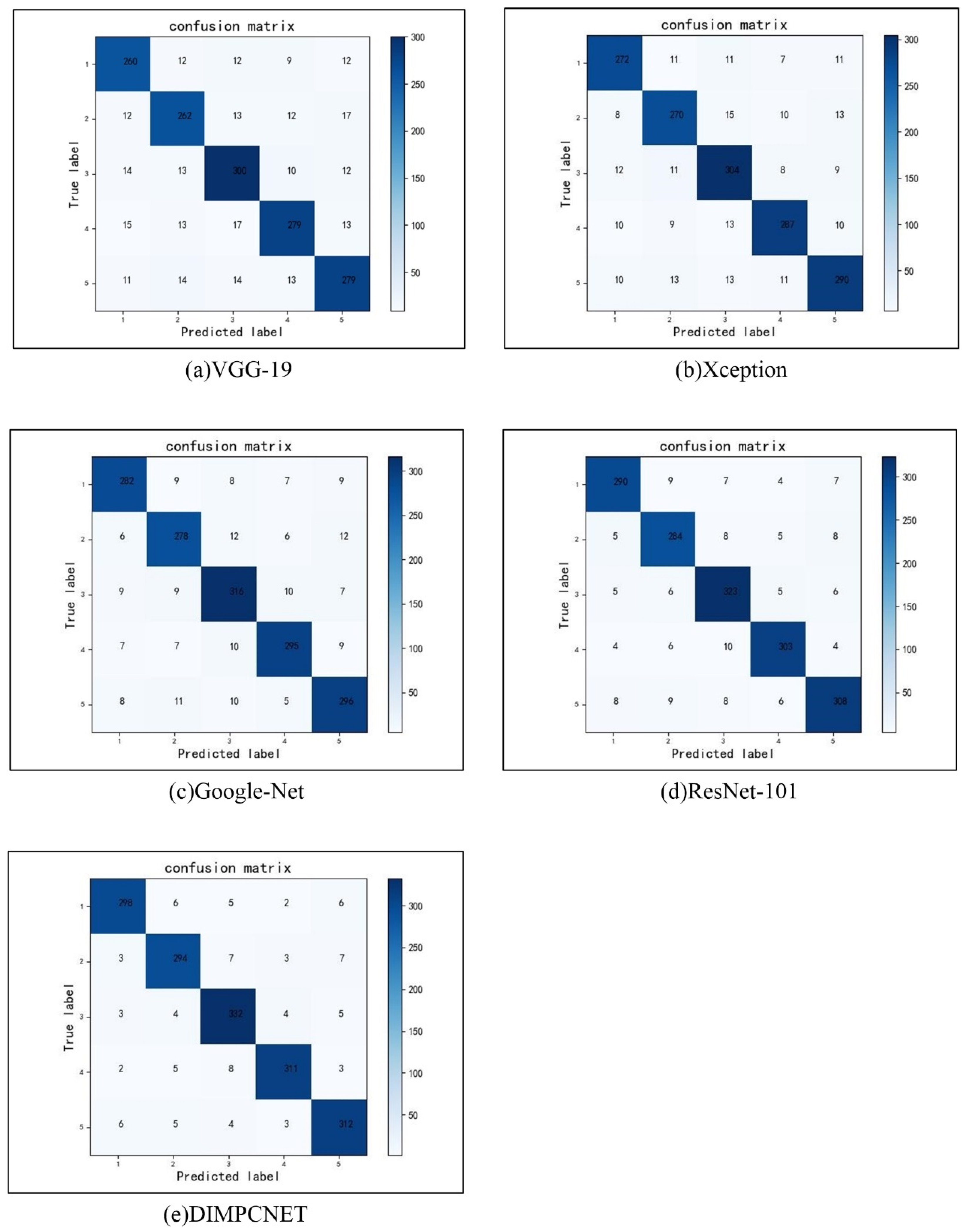
Figure 10 shows the confusion matrix using the DIMPCNET model and other network models to identify five tomato leaves (four diseased and one healthy leaf).
The confusion matrix calculated the accuracy of the DIMPCNET model in diagnosing healthy tomato leaves at more than 94%, especially in diagnosing early blight and gray leaf spot, two similar diseases, with an accuracy of 95% or even 96%. This is because the Inception dense connectivity module can extract and extract leaf disease features in multiple dimensions and scales, thus allowing to amplify the gap between classes and reduce the gap within classes to some extent. The diagnostic accuracy of leaf mold and gray mold was low but also reached 93.63% and 93.26%, respectively. The experimental result in Table 4 shows the clear superiority of the proposed PCBAM over other attention mechanisms, thus demonstrating the usefulness of PCBAM for solving complex backgrounds affecting recognition accuracy. In a word, DIMPCNET meets the precision required for real diagnostic tasks, and it achieves better experimental results than other general convolutional neural networks.

4.4. Comparison with the Latest Convolutional Neural Networks

Based on the dataset presented in this article, the DIMPCNET model was compared with advanced models such as Multi ScaleAlexNet, B-ARNet, DWOAM DRNet, and M-AORANet. The results are shown in Table 6. To explore the impact of DIMPCNET, each experiment was conducted using the same experimental environment. The DIMPCNET model proposed in this study achieved the highest accuracy, with an accuracy of 94.44%, as shown in Table 6. Compared with Multi ScaleAlexNet, B-ARNet, DWOAM DRNet, and M-AORANet, DIMPCNET has improved average accuracy by 2.48%, 8.95%, 2.03%, and 0.85%, respectively. The results indicate that the DIMPCNET model outperforms some of the latest crop disease classification models.

4.5. Ablation Experiment

To test the impact of DI and MPC branches on DIMPCNET network performance, four network structures VGG + VGG, VGG + DI, VGG + MPC, and DI + MPC, were respectively set up for ablation experiments. After 200 rounds of training, the other three structures had higher accuracy compared with the VGG + VGG structure, with DI + MPC having the highest accuracy, indicating that the DI and MPC module has a good contribution to the identification of tomato leaf diseases.
Table 7 illustrates how the four network architectures, VGG + VGG, VGG + DI, VGG + MPC, and DI + MPC, identify various tomato leaf diseases. The VGG + DI structure outperforms the VGG + VGG structure in recognizing five tomato leaf diseases, indicating that DI could extract multi-scale and multi-dimensional features. VGG + DI had higher accuracy in the recognition of early blight and gray leaf spot, indicating that DI could effectively alleviate the adverse effects caused by the uneven distribution of disease spots and the similarity of disease spots. Spatial location information of tomato leaf disease featured in images is essential for their identification accuracy. The attention mechanism has the ability to reduce extraneous background information and enhance the skill of recognizing objects. MPC module can use PCBAM mechanism to effectively alleviate the adverse impact of complex background on recognition effect. Therefore, this paper finally combines DI and MPC modules to form DIMPCNET, which can not only extract multi-dimensional features to enhance the recognition precision of related disorders but also alleviate the negative impact of complex background environments on disease recognition.

4.6. Attention Module Experiment

To verify the impact of PCBAM on network performance, the following models with MPC modules are validated: DIMNET, DIMNET + channel attention, DIMNET + spatial attention, DIMNET + CBAM, DIMNET + RCBAM, DIMNET + PCBAM. Indicators are shown in Table 8.
The reason why the MobileNet-V2 model is selected in the MPC module is because of its lightweight characteristics. After experimental comparison, the number of parameters of the Mobilenet-V2 model is only 2.34 × 10 6 , which is reduced by 5.209 × 10 7 compared with 5.443 × 10 7 of InRES-V2 model. Furthermore, the accuracy is almost as good as InRES-V2, which is an ideal lightweight model for pest recognition. The accuracy is improved by adding various attention modules to DIMNET. Among them, the model with the addition of PCBAM has the highest recognition accuracy in both top1 accuracy and other aspects, and the improvement of accuracy is very stable, which is 5.22 percentage points higher than the DIMNET. Thus, the efficiency and robustness of PCBAM have been proven once again.

4.7. Effectiveness of DIMPCNET on Other Leaf Disease Datasets

We performed experiments on a widely used dataset of grape leaf diseases to examine the generalizability of the proposed DIMPCNET model. The public dataset includes 2750 images of grapes plant diseases, including leaf blight, black measles, black rot, and brown spot. A sample image is shown in Figure 11.
According to Table 9, the average recognition accuracy of the DIMPCNET model for the four types of grape leaves is 97.24%, which is 2.8% better than the self-collected tomato leaf disease dataset. This is mainly because there are only four categories; another reason is that it is a public dataset with no complex background. Then, the average accuracy of the DIMPCNET model is improved by 10.33%, 9.08%, 4.97%, and 1.38% compared with the VGG-19, Xception, GoogleNet, and ResNet-101 models on the grape leaf disease dataset. Furthermore, this model also has the shortest recognition time of 31.42 ms for grape leaf images, which is 0.55 ms faster than the Xception model, which is second in order. According to the above analysis, the established model has the greatest precision and recognition speed in the process of identifying grape disease leaves, which indicates that the model is very worth promoting.

5. Conclusions and Prospect

In a variety of challenging situations, the newly designed tomato leaf disease classification system demonstrated excellent performance. It successfully solves the problem of complex backgrounds in images of tomato leaf disease taken in natural environments, as well as the significant differences between the same class of tomato leaf disease and the small differences in some diseases due to similar characteristics. The system shows strong robustness in dealing with these factors.
  • This study proposes the utilization of DIMPCNET for the identification of tomato leaf diseases. DIMPCNET is capable of efficiently extracting multi-dimensional and multi-scale features from diseased leaves, effectively addressing the challenges posed by complex background environments and the similarity of disease spots. Notably, DIMPCNET employs a unique two-branch classification structure, where each branch utilizes basic convolutional neural networks as feature extractors. The branches can be symmetric or asymmetric. Following feature extraction, a bilinear pooling method is employed to fuse the features. The DIMPCNET method demonstrates high accuracy in image classification tasks, outperforming traditional convolutional neural networks;
  • To combat the challenge of low precision in identifying pests and diseases with fine-grained multi-classification, a novel approach has been developed. The existing CBAM module, which utilizes serial connections, has been enhanced by introducing a parallel PCBAM attention module. This new module aims to address the interference problem caused by serial connections and improve the accuracy of recognition. By leveraging the parallel structure, the proposed solution aims to minimize interference and enhance the precision of pest and disease identification;
  • In order to assess the effectiveness and robustness of the PCBAM module, a comprehensive analysis was conducted to compare its recognition performance with other attention mechanisms in the DIMNET model. The recognition abilities of channel attention, spatial attention, CBAM, RCBAM, and PCBAM were thoroughly evaluated and compared. The results unequivocally demonstrate that the PCBAM module outperforms other attention mechanisms in accurately classifying diseases with fine-grained details. Furthermore, it exhibits remarkable generalization capabilities across different convolutional neural network models. These findings underscore the efficacy of the PCBAM module in precisely identifying and categorizing diseases, thus making it a valuable asset in the field of agricultural disease management;
  • Compared with the current popular classification method of tomato leaf disease, our recognition accuracy was 94.44%, and the F1 value was 0.9475. This method achieves better performance. It has obvious advantages in that it can effectively remove image noise and reduce the negative impact of complex background environments and disease similarity on disease recognition so as to effectively prevent and control tomato diseases and improve tomato yield;
  • At present, we only consider one disease on a single leaf, but if there are multiple diseases on a single leaf, how to identify them can be seen as a future direction. Next, we will further simplify the training process and consider improving the efficiency of the model. In addition, considering the shortcomings of relying solely on image modality to complete the tomato leaf disease recognition process, we plan to consider using a richer multi-modal dataset to achieve tomato leaf disease recognition.

Author Contributions

D.P.: Writing—original draft, Visualization. W.L.: Validation, Conceptualization. H.Z.: Supervision, Funding acquisition. G.Z.: Writing-review and editing C.C.: Software, Investigation. All authors have read and agreed to the published version of the manuscript.

Funding

This research was funded by the National Natural Science Foundation of China (6170344 grant).

Data Availability Statement

Data is available upon request.

Acknowledgments

We are grateful to all members of the Plant Protection Research Institute, Academy of Agricultural Sciences, for their advice and assistance in the course of this research.

Conflicts of Interest

The authors affirm that they do not have any recognized financial issues of interest or personal ties that could affect the work reported here.

References

  1. Kong, J.; Wang, H.; Wang, X.; Jin, X.; Fang, X.; Lin, S. Multi-stream hybrid architecture based on cross-level fusion strategy for fine-grained crop species recognition in precision agriculture. Comput. Electron. Agric. 2021, 185, 106134. [Google Scholar] [CrossRef]
  2. Shao, W.; Liu, L.; Jiang, J.; Yan, Y. Low-light-level image enhancement based on fusion and Retinex. J. Mod. Opt. 2020, 67, 1190–1196. [Google Scholar] [CrossRef]
  3. Qin, Y.; Luo, F.; Li, M. A Medical Image Enhancement Method Based on Improved Multi-Scale Retinex Algorithm. J. Med. Imaging Health Inform. 2020, 10, 152–157. [Google Scholar] [CrossRef]
  4. Liu, J.; Wang, S.; Wang, X.; Ju, M.; Zhang, D. A Review of Remote Sensing Image Dehazing. Sensors 2021, 21, 3926. [Google Scholar] [CrossRef]
  5. Chen, X.; Zhang, P.; Quan, L.; Yi, C.; Lu, C. Underwater image enhancement based on deep learning and image formation model. arXiv 2021, arXiv:2101.00991. [Google Scholar]
  6. Wu, W.; Weng, J.; Zhang, P.; Wang, X.; Yang, W.; Jiang, J. URetinex-Net: Retinex-Based Deep Unfolding Network for Low-Light Image Enhancement. In Proceedings of the IEEE/CVF Conference on Computer Vision and Pattern Recognition, New Orleans, LA, USA, 19–20 June 2022; pp. 5901–5910. [Google Scholar]
  7. Kaur, K.; Jindal, N.; Singh, K. Fractional derivative based Unsharp masking approach for enhancement of digital images. Multimed. Tools Appl. 2020, 80, 3645–3679. [Google Scholar] [CrossRef]
  8. Hou, Y.; Li, Q.; Zhang, C.; Lu, G.; Ye, Z.; Chen, Y.; Wang, L.; Cao, D. The State-of-the-Art Review on Applications of Intrusive Sensing, Image Processing Techniques, and Machine Learning Methods in Pavement Monitoring and Analysis. Engineering 2020, 7, 845–856. [Google Scholar] [CrossRef]
  9. Oktavianto, B.; Purboyo, T.W. A study of histogram equalization techniques for image enhancement. Int. J. Appl. Eng. Res. 2018, 13, 1165–1170. [Google Scholar]
  10. Li, P.; Huang, Y.; Yao, K. Multi-algorithm Fusion of RGB and HSV Color Spaces for Image Enhancement. In Proceedings of the 2018 37th Chinese Control Conference (CCC), Wuhan, China, 25–27 July 2018. [Google Scholar] [CrossRef]
  11. Land, E.H.; McCann, J.J. Lightness and Retinex Theory. J. Opt. Soc. Am. 1971, 61, 1–11. [Google Scholar] [CrossRef]
  12. Jobson, D.; Rahman, Z.; Woodell, G. Properties and performance of a center/surround retinex. IEEE Trans. Image Process. 1997, 6, 451–462. [Google Scholar] [CrossRef]
  13. Hu, W.W.; Wang, R.G.; Fang, S.; Hu, Q. Retinex image enhancement algorithm based on bilateral filtering. Graph. J. 2010, 31, 104–109. [Google Scholar]
  14. Zhang, X.; Zhao, L. Image enhancement algorithm based on improved Retinex. J. Nanjing Univ. Sci. Technol. 2016, 40, 24–28. [Google Scholar]
  15. Tan, L.; Chen, Y.; Zhang, W. Multi-focus Image Fusion Method based on Wavelet Transform. J. Phys. Conf. Ser. 2019, 1284, 012068. [Google Scholar] [CrossRef] [Green Version]
  16. Li, X.; Cong, Z.; Zhang, Y. Rail Track Edge Detection Methods Based on Improved Hough Transform. In Proceedings of the IEEE International Conference on Power Electronics, Computer Applications (ICPECA), Shenyang, China, 22–24 January 2021; pp. 12–16. [Google Scholar]
  17. Donoho, D. De-noising by soft-thresholding. IEEE Trans. Inf. Theory 1995, 41, 613–627. [Google Scholar] [CrossRef] [Green Version]
  18. Jianhui, X.; Li, T. Image Denoising Method Based on Improved Wavelet Threshold Transform. In Proceedings of the 2019 IEEE Symposium Series on Computational Intelligence (SSCI), Xiamen, China, 6–9 December 2019; pp. 1064–1067. [Google Scholar] [CrossRef]
  19. Lei, S.; Lu, M.; Lin, J.; Zhou, X.; Yang, X. Remote sensing image denoising based on improved semi-soft threshold. Signal Image Video Process. 2020, 15, 73–81. [Google Scholar] [CrossRef]
  20. Panchal, P.; Raman, V.C.; Mantri, S. Plant diseases detection and classification using machine learning models. In Proceedings of the 2019 4th International Conference on Computational Systems and Information Technology for Sustainable Solution (CSITSS), Bengaluru, India, 20–21 December 2019; IEEE: Piscataway, NJ, USA, 2019; Volume 4, pp. 1–6. [Google Scholar]
  21. Ramesh, S.; Hebbar, R.; Niveditha, M.; Pooja, R.; Shashank, N.; Vinod, P.V. Plant disease detection using machine learning. In Proceedings of the 2018 International Conference on Design Innovations for 3Cs Compute Communicate Control (ICDI3C), Bengaluru, India, 24–26 April 2018; pp. 41–45. [Google Scholar]
  22. Rashmi, N.; Shetty, C. A Machine Learning Technique for Identification of Plant Diseases in Leaves. In Proceedings of the 6th International Conference on Inventive Computation Technologies (ICICT), Lalitpur, Nepal, 26–28 April 2023; pp. 481–484. [Google Scholar]
  23. Reza, Z.N.; Nuzhat, F.; Mahsa, N.A.; Ali, M.H. Detecting Jute Plant Disease Using Image Processing and Machine Learning. In Proceedings of the 3rd International Conference on Electrical Engineering and Information Communication Technology (ICEEICT), Dhaka, Bangladesh, 22–24 September 2016; pp. 1–6. [Google Scholar]
  24. Akhtar, A.; Khanum, A.; Khan, S.A.; Shaukat, A. Automated Plant Disease Analysis (APDA): Performance Comparison of Machine Learning Techniques. In Proceedings of the 2013 11th International Conference on Frontiers of Information Technology, Islamabad, Pakistan, 16–18 December 2013; pp. 60–65. [Google Scholar] [CrossRef]
  25. Wang, J.; Ning, F.; Lu, S. Study on apple leaf disease identification method based on support vector machine. Shandong Agric. Sci. 2015, 47, 122–125. [Google Scholar]
  26. Qin, F.; Liu, D.X.; Sun, B.D. Recognition of four different alfalfa leaf diseases based on image processing technology. China Agric. Univ. 2016, 21, 65–75. [Google Scholar]
  27. Xie, C.; He, Y. Spectrum and Image Texture Features Analysis for Early Blight Disease Detection on Eggplant Leaves. Sensors 2016, 16, 676. [Google Scholar] [CrossRef] [Green Version]
  28. Chai, A.L.; Li, B.J.; Shi, Y.X. Recognition of tomato foliage disease based on computer vision technology. Acta Hortic. Sinica 2010, 37, 1423–1430. [Google Scholar]
  29. Zhang, Y.L.; Yuan, H.; Zhang, Q.Q. Apple leaf disease recognition method based on color feature and difference histogram. Jiangsu Agric. Sci. 2017, 45, 171–174. [Google Scholar]
  30. Xia, Y.Q.; Bing, W.; Jun, Z. Identification of wheat leaf disease based on random forest method. J. Graph. 2018, 39, 57. [Google Scholar]
  31. Wu, Y. Identification of Maize Leaf Diseases based on Convolutional Neural Network. J. Phys. Conf. Ser. 2021, 1748, 032004. [Google Scholar] [CrossRef]
  32. Ding, R.; Zhou, P. Identification of typical crop leaf diseases based on convolutional neural network. Packag. J. 2018, 10, 74–80. [Google Scholar]
  33. Alom, M.Z.; Taha, T.M.; Yakopcic, C.; Westberg, S.; Sidike, P.; Nasrin, M.S.; Asari, V.K. The history began from alexnet: A comprehensive survey on deep learning approaches. arXiv 2018, arXiv:1803.01164. [Google Scholar]
  34. Guo, X.Q.; Fan, T.J.; Shu, X. Tomato leaf disease image recognition based on improved Multi-scale AlexNet. Trans. Chin. Soc. Agric. Eng. 2019, 35, 162–169. [Google Scholar]
  35. Ni, L.; Zou, W. Recognition of animal species based on improved Xception by SE module. Navig. Control 2020, 19, 106–111. [Google Scholar]
  36. Zhang, S.; Huang, W.; Zhang, C. Three-channel convolutional neural networks for vegetable leaf disease recognition. Cogn. Syst. Res. 2019, 53, 31–41. [Google Scholar] [CrossRef]
  37. Zhang, S.; Zhang, S.; Zhang, C.; Wang, X.; Shi, Y. Cucumber Leaf Disease Identification with Global Pooling Dilated Con-volutional Neural Network. Comput. Electron. Agric. 2019, 162, 422–430. [Google Scholar] [CrossRef]
  38. Gulzar, Y. Fruit Image Classification Model Based on MobileNetV2 with Deep Transfer Learning Technique. Sustainability 2023, 15, 1906. [Google Scholar] [CrossRef]
  39. Mamat, N.; Othman, M.F.; Abdulghafor, R.; Alwan, A.A.; Gulzar, Y. Enhancing Image Annotation Technique of Fruit Clas-sification Using a Deep Learning Approach. Sustainability 2023, 15, 901. [Google Scholar] [CrossRef]
  40. Aggarwal, S.; Gupta, S.; Gupta, D.; Gulzar, Y.; Juneja, S.; Alwan, A.A.; Nauman, A. An Artificial Intelligence-Based Stacked Ensemble Approach for Prediction of Protein Subcellular Localization in Confocal Microscopy Images. Sustainability 2023, 15, 1695. [Google Scholar] [CrossRef]
  41. Gulzar, Y.; Hamid, Y.; Soomro, A.B.; Alwan, A.A.; Journaux, L. A Convolution Neural Network-Based Seed Classification System. Symmetry 2020, 12, 2018. [Google Scholar] [CrossRef]
  42. Chen, X.; Zhou, G.; Chen, A.; Yi, J.; Zhang, W.; Hu, Y. Identification of tomato leaf diseases based on combination of ABCK-BWTR and B-ARNet. Comput. Electron. Agric. 2020, 178, 105730. [Google Scholar] [CrossRef]
  43. Zhang, Y.; Huang, S.; Zhou, G.; Hu, Y.; Li, L. Identification of tomato leaf diseases based on multi-channel automatic orien-tation recurrent attention network. Comput. Electron. Agr. 2023, 205, 107605. [Google Scholar] [CrossRef]
  44. Sun, J.; Tan, W.; Mao, H.; Wu, X.; Chen, Y.; Wang, L. Recognition of multiple plant leaf diseases based on improved convo-lutional neural network. Trans. Chin. Soc. Agric. Eng. 2017, 33, 209–215. [Google Scholar]
  45. Gibran, M.; Wibowo, A. Convolutional Neural Network Optimization for Disease Classification Tomato Plants Through Leaf Image. In Proceedings of the 5th International Conference on Informatics and Computational Sciences (ICICoS), Semarang, Indonesia, 24–25 November 2021; pp. 116–121. [Google Scholar]
  46. Cai, C.; Wang, Q.; Cai, W.; Yang, Y.; Hu, Y.; Li, L.; Wang, Y.; Zhou, G. Identification of grape leaf diseases based on VN-BWT and Siamese DWOAM-DRNet. Eng. Appl. Artif. Intell. 2023, 123, 106341. [Google Scholar] [CrossRef]
  47. Kong, J.; Wang, H.; Yang, C.; Jin, X.; Zuo, M.; Zhang, X. A Spatial Feature-Enhanced Attention Neural Network with High-Order Pooling Repre-sentation for Application in Pest and Disease Recognition. Agriculture 2022, 12, 500. [Google Scholar] [CrossRef]
  48. Mohideen, S.K.; Perumal, S.A.; Sathik, M.M. Image De-Noising Using Discrete Wavelet Transform. Int. J. Comput. Sci. Netw. Secur. 2008, 8, 213–216. [Google Scholar]
  49. Fang, S.; Yang, J.R.; Cao, Y.; Wu, P.F.; Rao, R.Z. Local Multi-Scale Retinex Algorithm for Image Guided Filtering. J. Image Graph. 2012, 17, 748–755. [Google Scholar]
  50. Ouhami, M.; Es-Saady, Y.; Hajji, M.E.; Hafiane, A.; Canals, R.; Yassa, M.E. Deep transfer learning models for tomato disease detection. In Proceedings of the 9th International Conference, ICISP 2020, Marrakesh, Morocco, 4–6 June 2020; pp. 65–73. [Google Scholar]
  51. McNeely-White, D.; Beveridge, J.R.; Draper, B.A. Inception and ResNet features are (almost) equivalent. Cogn. Syst. Res. 2019, 59, 312–318. [Google Scholar] [CrossRef]
  52. Li, Z.; Yang, Y.; Li, Y.; Guo, R.; Yang, J.; Yue, J. A solanaceae disease recognition model based on SE-Inception. Comput. Electron. Agric. 2020, 178, 105792. [Google Scholar] [CrossRef]
  53. Jangapally, T. Image Classification Using Network Inception-Architecture & Applications. JIDPTS 2021, 4, 6–9. [Google Scholar]
  54. Zhang, Y.; Hou, Y.; OuYang, K.; Zhou, S. Multi-scale signed recurrence plot based time series classification using inception architectural networks. Pattern Recognit. 2021, 123, 108385. [Google Scholar] [CrossRef]
  55. Li, S.; Ma, H. A Siamese inception architecture network for person re-identification. Mach. Vis. Appl. 2017, 28, 725–736. [Google Scholar] [CrossRef]
  56. Howard, A.G.; Zhu, M.; Chen, B.; Kalenichenko, D.; Wang, W.; Weyand, T.; Andreetto, M.; Adam, H. MobileNets: Efficient Convolutional Neural Networks for Mobile Vision Applications. arXiv 2017, arXiv:1704.04861. [Google Scholar]
  57. Szegedy, C.; Wei, L.; Yangqing, J.; Sermanet, P.; Reed, S.; Anguelov, D.; Erhan, D.; Vanhoucke, V.; Rabinovich, A. Going deeper with convolutions. In Proceedings of the 2015 IEEE Conference on Computer Vision and Pattern Recognition (CVPR), Boston, MA, USA, 7–12 June 2015; pp. 1–9. [Google Scholar]
  58. Fu, J.; Zheng, H.; Mei, T. Look Closer to See Better: Recurrent Attention Convolutional Neural Network for Fine-Grained Image Recognition. In Proceedings of the 2017 IEEE Conference on Computer Vision and Pattern Recognition (CVPR), Honolulu, HI, USA, 21–26 July 2017; pp. 4476–4484. [Google Scholar]
  59. Hu, J.; Shen, L.; Sun, G. Squeeze-and-Excitation Networks. In Proceedings of the IEEE Conference on Computer Vision and Pattern Recognition (CVPR), Salt Lake City, UT, USA, 18–23 June 2018; pp. 7132–7141. [Google Scholar]
  60. Woo, S.; Park, J.; Lee, J.Y.; Kweon, I.S. CBAM: Convolutional block attention module. In Proceedings of the European Conference on Computer Vision, Munich, Germany, 8–14 September 2018. [Google Scholar] [CrossRef] [Green Version]
  61. Prado, J.; Yandun, F.; Torriti, M.T.; Cheein, F.A. Overcoming the Loss of Performance in Unmanned Ground Vehicles Due to the Terrain Variability. IEEE Access 2018, 6, 17391–17406. [Google Scholar] [CrossRef]
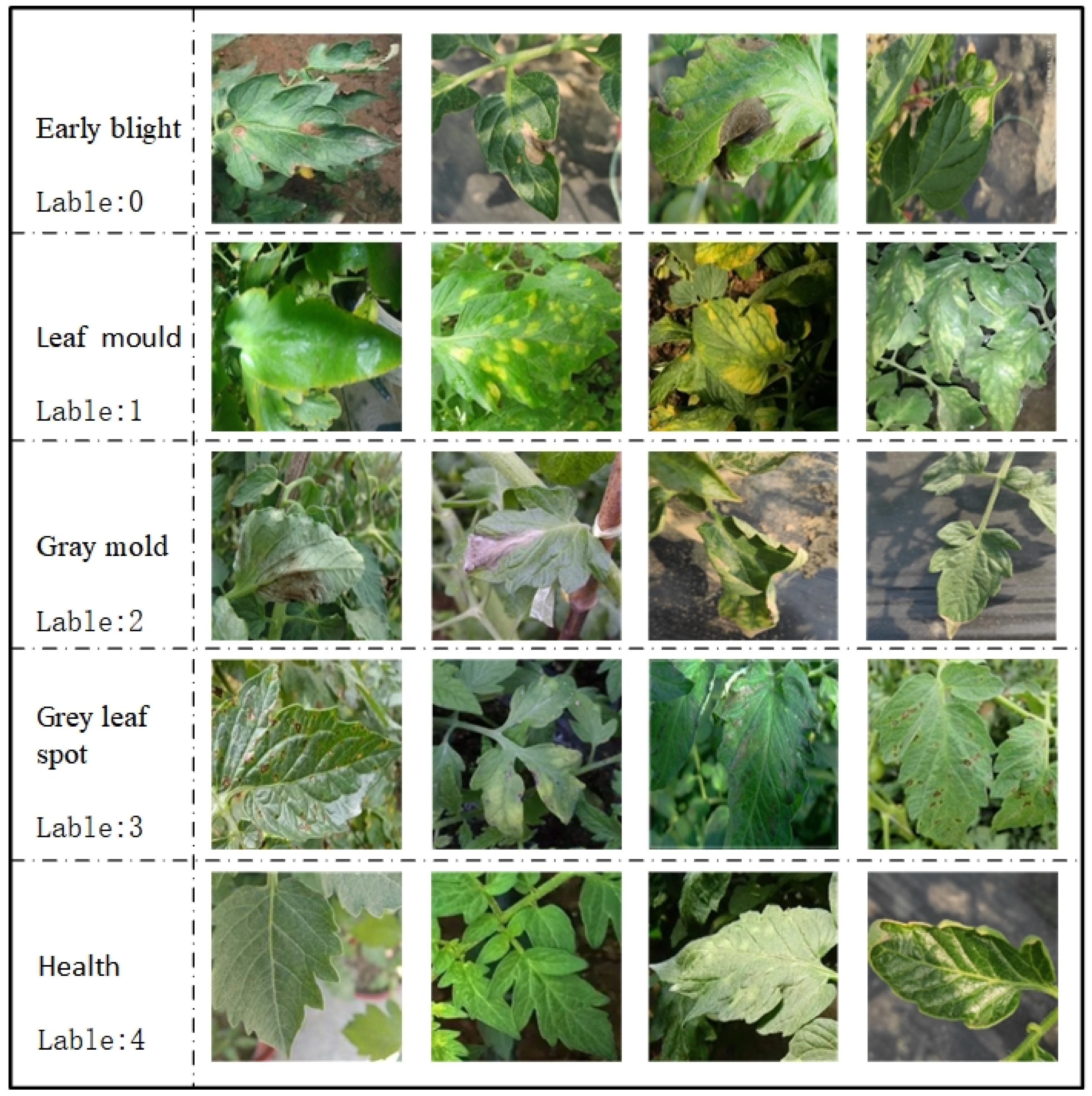
Figure 1. Image of diseased tomato leaves.
Agronomy 13 01812 g001
Figure 2. System functional structure diagram.
Agronomy 13 01812 g002
Figure 3. Partial enhanced image.
Agronomy 13 01812 g003
Figure 4. Flowchart of IBFTF image enhancement algorithm.
Agronomy 13 01812 g004
Figure 5. Original image and IBFTF enhanced image.
Agronomy 13 01812 g005
Figure 6. Overall model structure diagram.
Agronomy 13 01812 g006
Figure 7. Structure of the DI module.
Agronomy 13 01812 g007
Figure 8. Schematic diagram of the dense connectivity policy.
Agronomy 13 01812 g008
Figure 9. Schematic diagram of PCBAM structure.
Agronomy 13 01812 g009
Figure 10. Confusion matrix of identification results of different network models.
Agronomy 13 01812 g010
Figure 11. Grape leaf dataset:(a) black measles; (b) brown spot disease; (c) healthy leaves; (d) leaf blight.
Agronomy 13 01812 g011
Table 1. Tomato leaf disease dataset.
Disease TypeBefore Data EnhancementAfter Data EnhancementProportion
early blight312156019.04%
leaf mold314157019.16%
gray mold356178021.73%
grey leaf323161519.71%
health333166520.32%
Table 2. Experiment environment.
Experimental Environment ConfigurationParameter Values
Enhancement
CPUIntel(R) Xeon(R) Gold 6271C [email protected] GHz
GPUNVIDIA Tesla V100 GPU32 G
RAM32 G
Magnetic disk100 G
Deep learning frameworkPyTorch
Operating SystemWindows 10(64-bits)
OthersPython 3.7.1CUDA10.1
Table 3. Experiment parameter.
Parameter NameParameter Values
Image Size224 × 224
Batch size 60
Learning rate0.001
Magnetic disk100 G
Epoch200
Table 4. Accuracy of traditional network models.
ModuleInputPrecisionRecallF1 T A (ms) Accuracy (%)
VGG-192240.8333 0.85250.842733.5684.25
Xception2240.87180.87180.871832.9286.87
GoogleNet2240.90380.89520.899540.2689.56
ResNet-1012240.92950.91480.922039.5392.06
DIMPCNET2240.95510.94000.947531.6894.44
Table 5. Accuracy of network models in validation sets.
ModuleInputPrecisionRecallF1 T A (ms) Accuracy (%)
VGG-192240.8298 0.85080.840133.3984.06
Xception2240.86790.86480.866334.7986.12
GoogleNet2240.90110.88830.894738.4689.78
ResNet-1012240.92790.91090.919337.8792.71
DIMPCNET2240.94670.93370.940232.2193.82
Table 6. Accuracy of the latest network models.
ModuleInputPrecisionRecallF1 T A (ms) Accuracy (%)
Multi-ScaleAlexNet2240.9163 0.91590.913435.3491.96
B-ARNet2240.85720.85650.856833.8585.49
DWOAM-DRNet2242240.92810.92640.927236.62
M−AORANet2240.93690.93600.936438.6493.59
DIMPCNET2240.95510.94000.947531.6894.44
Table 7. Results of ablation experiments.
ModuleAccuracyF1 ScoreParam
(M)
Early BlightLeaf MoldGray MoldGrey Leaf SpotHealth
VGG + VGG 88.45%0.89570.87450.88710.90070.894954.02
VGG + DI91.44%0.92560.91570.91610.91950.903956.02
VGG + MPC92.68%0.93210.93350.92660.93120.920546.02
DI + MPC94.29%0.94690.93010.93840.94580.932648.02
Table 8. Experimental results of each attention module embedded in DIMNET (DI+MobileNet-V2).
NetworkTop1
Accuracy/%
Forward Propagation Time/msModel Size/
MB
Number of ParametersAccuracy↑
(↑, Percentage Increase)
DIMNET90.48%7.1856.1 47.34   ×   10 7
DIMNET+channel attention90.97%7.1886.8 48.97   ×   10 7 0.49%
DIMNET+spatial attention91.36%7.1586.1 47.33   ×   10 7 0.88%
DIMNET+CBAM93.21%7.3386.9 48.97   ×   10 7 2.73%
DIMNET+RCBAM92.38%7.3386.9 48.97   ×   10 7 1.90%
DIMNET+SE94.58%7.3392.6 49.13   ×   10 7 4.10%
DIMNET+PCBAM95.70%7.1586.9 45.76   ×   10 7 5.22%
Table 9. Experimental outcomes of each network model on grape leaf dataset.
GrapeInputPrecisionRecallF1TA (ms)Accuracy
VGG-192240.86390.87470.869331.9786.91
Xception2240.89250.87140.881831.9788.16
GoogleNet2240.92160.93090.926231.4292.27
ResNet-1012240.95950.95130.955433.2795.86
DIMPCNET2240.97560.97150.973531.4297.24
Disclaimer/Publisher’s Note: The statements, opinions and data contained in all publications are solely those of the individual author(s) and contributor(s) and not of MDPI and/or the editor(s). MDPI and/or the editor(s) disclaim responsibility for any injury to people or property resulting from any ideas, methods, instructions or products referred to in the content.