Abstract
The cultivation of pearl millet in India is experiencing important transformations. Here, we propose a new characterization of the pearl millet production environment using the latest available district level data (1998–2017), principal component analysis, and large-scale crop model simulations. Pearl millet cultivation environment can be divided in up to five environments (TPEs). The eastern part of the country (Rajasthan, Haryana, Uttar Pradesh) emerges as the only region where pearl millet cultivation has grown (+0.4 Kha/year), with important yield increase (+51 kg/ha/year), and potential surplus that are likely exported. Important reductions of pearl millet cultivated area in Gujarat (−4.5 Kha/year), Maharashtra and Karnataka (−4 Kha/year) are potentially due to economy-driven transition to other more profitable crops, such as cotton or maize. The potential rain increase could also accelerate this transition. With [0.15–0.61], the tested crop models reflected reasonably well the pearl millet production system in the A1 (North Radjasthan) and AE1 (South Rajastan and Haryana) TPEs covering the largest area (66%) and production share (59%), especially after the use of a new strategy for environment and management parameters calibration. Those results set the base for in silico system design and optimization in future climatic scenarios.
1. Introduction
Pearl millet is an important crop cultivated on about 30 million hectares (ha) in more than 30 countries [1]. In India, pearl millet is mainly cultivated under rain-fed conditions during the rainy season (kharif) and represented of the yearly cultivated surface during the period 1998–2017. Due to its capacity to use water efficiently and its heat tolerance, pearl millet is adapted to harsh climatic conditions where other crops fail to produce economic yield [2,3]. However, despite constant increases across the production area, with an average of 1161 kg/ha over 1998–2017, pearl millet yield remains low compared to other crops in the same regions (e.g., rice: 1967 kg/ha; maize: 1650 kg/ha). Moreover, limited market opportunities and minimal government support are important constraints for farmers to consider pearl millet for cultivation. Thus, pearl millet is mostly used for food and fodder [4] and it is under the constant pressure of changes in dietary patterns for crops, such as wheat or rice [5].
The sustainable intensification of complex agronomic systems like pearl millet cultivation in India with a wide range of weather conditions (e.g., low and high precipitation), soil type (e.g., from sandy to black vertisol), and/or socio-economic usages with many possible interactions [6], requires quantitative understanding of production environments. This quantification set the base to design context specific technologies [7,8,9]. Increasingly, crop simulation modelling (CSM) is used for environmental characterization (envirotyping) and the definition of target population of environments (TPE) [10,11,12,13,14]. A TPE is composed of environments (TPEs) with more homogeneous biophysical properties. Their identification and use for breeding help to reduce the GxE effect in selection [15,16]. Therefore, the TPE definition is a prerequisite for several important applications, such as the optimization of multi-location breeding trials sampling.
The initial characterization of pearl millet cultivation in India dates to 1979 when the National Agricultural Research Project divided the environment into zones A and B. Later, zone A was split into A1 and A parts [17,18] (Figure 1A). This zonation mostly relies on the yearly rain pattern and is still considered today as a reference in many pearl millet breeding programs. According to this zonation, pearl millet is cultivated under low precipitations (<400 mm/year) in the north of Rajasthan classified as A1 zone, in the neighbouring regions of south Rajasthan, Haryana, Gujarat, and Uttar Pradesh termed as A zone (>400 mm/year), and central Western India referred as B zone (>400 mm/year).
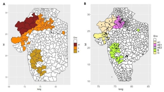
Figure 1.
(A) Selected 62 districts representing 90% of the total kharif pearl millet area over the period 1998–2017. The districts are coloured according to the reference rain and geography criteria (A1: < 400 mm/year; A: North > 400 mm/year; B: South > 400 mm/year) (B) New TPE with All India Coordinated research project (AICRP) pearl millet testing sites during kharif and Summer season 2017.
Except for the work by Gupta et al. [19], no notable revision of the TPE has been proposed recently. That work supported the absence of difference between the A1 and A zones, which was equivalent to the initial zonation. However, this analysis was based on yield data of well-managed improved varieties breeding trials. We suggest that a revision of the Indian pearl millet TPE integrating a wider source of information should better capture the complexity of this system [6]. This revision is the main objective of the article.
CSM progressively became one of the most important tools for environmental characterization [20,21]. CSMs are in silico representations of natural systems captured by a series of equations [22]. These equations express agronomic traits such as yield as a function of environmental inputs (e.g., temperature, soil water potential), management practices (e.g., irrigation, fertilization) and crop characteristics (e.g., phenology, canopy growth, biomass partitioning) [23]. CSM reconstruct the soil–plant–atmosphere continuum of a system at the plot level. Those simulation can be scaled up across spatio-temporal scales (e.g., region) to identify TPEs with similar biophysical properties forming the TPE [16,24].
Recently, increases in computer power created the opportunity to run large-scale simulations to extensively explore the properties of agronomic systems (e.g., Ronanki et al. [24]). The second objective of the article is to present an innovative strategy based on large-scale crop model simulations to support the revision of the pearl millet TPE. This strategy helped us to gather extra information about the locations where pearl millet is cultivated, as well as estimating the influence of different parameters on the yield (sensitivity analysis). This article also allowed us to evaluate a new crop model characterized by an improved algorithm to describe pearl millet tillering [25,26]. Since tillering is critical for pearl millet adaptation to drought-prone environments, the evaluation of this updated CSM tool in the new TPEs is an important prerequisite to design crops and management strategies for the current and future climates in the target geographies. It will also support pearl millet crop model development, which remains an under-researched area [27,28,29].
2. Materials and Methods
Figure 2 is a visualization of the material and methods workflow. The materials and methods is divided in three parts. The first one describes the data used for the TPE determination, (a) ICRISAT district level data (DLD); (b) Nasapower synthetic weather data [30]; and (c) parameters derived from crop model simulations (Table 1). The second part describes the methodology to determine the TPE; and the third part the crop modelling strategy to (a) infer parameters of the system using large-scale simulation, (b) use those simulations to evaluate the crop model prediction (st)ability within the identified TPEs, and (c) determine the relative influence on yield of the tested parameter in the new TPEs.
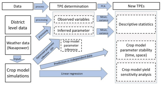
Figure 2.
Materials and Methods workflow.

Table 1.
Description of the data used and its origin (district level data—DLD, Nasapower weather data, crop model inferred parameter) and their usage in the principal component analysis (PCA).
2.1. Data
2.1.1. District Level Data (DLD)
The DLD (http://data.icrisat.org/dld/ (accessed on 1 April 2023)) is an open-source database about Indian agriculture at the district level that contains data originally compiled by the Indian directorate of economics and statistics (https://desagri.gov.in/ (accessed on 1 April 2023)). From this database, we extracted the most recently available 20 years (1998–2017) of data on pearl millet cultivated area, production, and yield during the rainy season (kharif, Table 1). We identified 62 districts representing of the total cultivated area during the period (Figure 1A). Consequently, the other pearl millet system characteristics were evaluated for these districts over the selected period. In these 62 districts, we used the area, production, and yield average (1998–2017), and further calculated their increase or decrease over a year (i.e., “trend”) as their linear regression coefficient estimate over several years. For area and production, we also estimated their average share as the proportion of pearl millet area (production) compared to other crops. We estimated the area and production trends as the linear regression coefficient of the share over years (1998–2017). We complemented the data with the major soil type for each district [31], the percentage of pearl millet area under irrigation, the amount of applied nitrogen (fertilizer) per hectare for all crops (not specific to pearl millet), and the price at harvest per 100 kg (Table 1). For irrigation, fertilizer, and price, we also estimated the trend as their linear regression coefficient estimate over several years. For example, the increase/decrease in irrigated surface over years.
2.1.2. Weather Data—Nasapower
For weather, we used the synthetic data provided by Nasapower [30], which has been shown to sufficiently represent the observed weather data [24,32]. The selected data contained daily precipitation (Figure S1), minimum and maximum temperature (Figure S2), and solar radiation, which are the only requested crop model input variables. We used the R package apsimx [33] to extract the data for a point located at the center of each district. We calculated the cumulative rain during kharif season (15 June–15 September), as well as its trend and variance over years (Table 1). We also calculated the temperature trends. The rain and temperature trends were calculated as the linear regression coefficient over years.
2.2. TPE Determination
The agronomic district level data and the weather data were complemented by information about the system, such as the most probable soil depth or sowing date estimated through the crop model simulations (Table 1, see next sections). Those data were used to perform a principal component analysis (PCA). For area and production, we used the within district proportion (share) rather than the absolute value. We used a k-mean clustering approach [34] with the number of clusters varying between three to eight. After the discussion with practitioners, the results with three to five clusters looked the most realistic one given the required insight on homogeneity of pearl millet production environments. The districts grouped in the same cluster were considered as more homogeneous than the one in other clusters and formed the new TPEs.
2.3. Crop Model Inference Strategy
We present a strategy based on extensive simulations to evaluate the crop model behavior and derive information about the system. By generating those outputs, we could (a) evaluate the crop model ability to reconstruct the pearl millet production at the district level; (b) estimate environment (soil) and management parameters that support the system characterization; and (c) determine the main constraints of the system.
2.3.1. Crop Model Description
We used two versions of the Agricultural Production Systems Simulator (APSIM) pearl millet model [35]. The default model was a first attempt to integrate pearl millet in APSIM by modelling dynamic tillers as an intercrop of the different axes [36,37]. The second model extended the default model by integrating more recent biological knowledge [38,39]. It integrated a modification of the canopy developmental dynamics, which was necessary to build an algorithm reproducing the growth of tillers driven by the carbohydrates supply/demand with genotype-specific tillering propensity as proposed by Alam et al. [25], Alam et al. [26]. For a more detailed description of the two crop models, see [40].
2.3.2. Simulations Setup
The CSM were run in APSIM 7.10 [35]. The simulations were initiated on the 15 April, two months before the hypothetical sowing date to potentially utilize the early rains, if these would occur. Inside the defined sowing window, The crop model was set to initiate the crop when at least 8.5 mm of rain was accumulated within five days and the soil contained a minimum of 25 mm of available water. If those conditions were not met, the crop was sown on the last day. Crops were sown at a 3 cm depth. No tillage operation was performed before sowing. Fertilization and irrigation were performed according to the simulation values (Table 2). The crop was harvested (some grain yield was recorded) on the day it reached the “ripe” or “dead” phenological stage before the end of the simulation (maximum four months after sowing). For each combination of district and parameter, the simulation was re-initialized after each season (year).
Table 2.
Crop model environment and management parameter ranges.
2.3.3. Crop Model Calibration
From a general point of view, crop model calibration consists of estimating model parameters by fitting the model to the observed data [41]. The crop models were calibrated for genotype parameters in previous studies [36,37,40]. A challenge for crop model prediction is the determination of all parameter values corresponding to the studied system [42]. In addition to the genotype-related parameters, crop models are generally also defined by environment parameters (e.g., soil parameters), and management parameters [43]. In controlled field experiments, parameters such as the soil type or the plant density can be assessed. However, for larger scale predictions, as in our case at the district level, the parameters are more uncertain and need to be generalized [44]. Those uncertainties reduce the crop model prediction accuracy [45]. A standard approach is to determine the most likely parameters after a literature review and discussions with specialists [13,32]. We called this approach an informed strategy. To evaluate the latter, we determined in each of the original zones (A1, A, and B) the most likely parameter values using available data and the literature (Table S1).
The informed strategy can, however, reach some limits, for example due to the dynamic nature of complex agronomic systems, especially in heterogeneous marginalized systems, such as pearl millet in India; those changes are accelerated by climate change. Therefore, in the present study, we investigated the feasibility to calibrate crop models for important environment and management (ExM) parameters by considering them as a random variables that were floated in large-scale simulations, which would allow the user to estimate the most likely values for those parameters. We called this approach ExM parameter calibration (see Section 2.3.5).
2.3.4. Crop Model ExM Parameters Space
To evaluate the crop model in different parameter configurations, we defined the ranges of possible values for important ExM parameters (Table 2). We determined the relevant ranges after DLD analysis, review of the literature, and discussions with experts. For the soil parameters, we selected generic soil textures that corresponded to the majority soil type information from the DLD [31], which potentially constitutes the most precise information about soil type at the district level in India. This information was crossed with data from the ISRIC global database (https://www.isric.org (accessed on 1 April 2023)). We selected three soil textures, sandy, loam, and clay soils, representing the majority soil types (Pssament, Inceptisol, and Vertisol) observed in the pearl millet tract (Figure S3). We used the generic APSIM soil profiles corresponding to these types of soils [46]. These soils are characterized by plant available water capacity (PAWC) of 0.6, 0.9, and 1.3 mm of water per cm of soil, respectively, [47]. For each soil type we defined three soils with depths fixed at 60, 120, or 180 cm—representing shallow, medium, and deep soil profiles.
According to the available literature [48] and the practitioners’ information, pearl millet is generally sown around the first two weeks (1–15) of July. However, it is conditioned by the onset of the rains. Considering these, we also defined an early (16–30 June) and a late sowing window (16–30 July). In terms of plant density, farmer practices and agronomic guidelines documented values between 10 and 22 plants/m2 with lower densities recommended for the more arid zones [3,49]. Therefore, we used 12, 18, and 24 plants/m2. In terms of variety usage, few systematic data collections (e.g., Asare-Marfo et al. [50]) and information from ICRISAT breeders provided us general information, such as the importance of landrace in the A1 zone and the higher adoption of improved varieties in other regions [51]. Therefore, we used three varieties, landrace, HHB67-2, and 9444, representing the generic pearl millet crop types used in India. The landrace is representative of local varieties used in the western part of Rajasthan [36]. HHB67-2 and 9444 are two hybrids with short and long duration, respectively, [40]. The 9444 variety was only parameterized in the updated crop model.
With yearly data at the district level, the DLD certainly represent the most reliable source of information about irrigation and fertilization practices in the Indian pearl millet system. These data indicated that in the selected districts, during kharif the average quantity of Nitrogen (N) used ranges from 15.5 kg/ha in the A1 zone to 82.8 in the B zone. To approximate these ranges, we selected (a) no fertilization; (b) 30 kg/ha as basal dose +30 kg/ha at 20 days; and (c) 50 kg/ha as basal dose +50 kg/ha at 20 days. Similarly, for irrigation, the DLD indicated that pearl millet is mostly rain-fed with on average of the cultivated surface under irrigation in the A1 zone and in the A zone. Therefore, we used (a) no irrigation, (b) limited irrigation applied when the fraction of available soil water (ASW) is below 0.25, and (c) full irrigation when ASW fraction is below 0.5.
2.3.5. Crop Model ExM Parameter Calibration
Crop models can be seen as a function that predicts an output such as yield given the parameters (e.g., the level of irrigation) [42]. Assuming no error in the model and the observations, one can estimate the likelihood of a selected parameter by calculating the crop model output for different values and comparing the output with real observations . The parameter values resulting in the smallest difference (–) should be the most likely (Figure S4). In our case, for each of the 3645 unique ExM parameter combinations (Table 2) we predicted the yield in each district every years. We determined the most likely parameter combination as the one with the highest Pearson correlation () between yearly predicted and observed values of yield. Using those results we could obtain continuous values for the estimated parameters by calculating the weighted average of the parameter value from the best . The weights were proportional to the value.
2.3.6. Crop Model Evaluation and Parameter Stability over Time and Space
We evaluated the crop model general prediction ability for each district using between the complete observed yield time series (1998–2017) and the predictions obtained with the estimated ExM parameters. We compared the crop model prediction ability obtained with the estimated ExM parameters to the one obtained with the informed strategy. This first scenario was termed overall. The simulation output also allowed us to evaluate the capacity of estimated ExM parameters to predict outcome in pseudo-independent data over time, and over space (parameter stability). For that purpose, we split the yield observation between present years (1998–2007) and future years (2008–2017), as well as between a training and a test neighbour districts (closest district by at least 150 km). In a second scenario designed to test the effect of time (time effect), we estimated the ExM parameters for a district using the present years and then predicted the yield in the future years for the same district. In a third scenario, designed to test the difference of location effect (location effect), we used the parameters determined in the training district in the present years to predict the yield of the test neighbour district in the same years. The prediction abilities over time, and over space were also estimated by between the predictions and the observations.
2.3.7. Crop Model Sensitivity Analysis
The generated crop model output allowed us to perform a sensitivity analysis to evaluate the effect of the input parameters on yield in each newly determined TPE. We used linear regressions of the predicted yield (output) on the input parameters (e.g., ) and weather parameters (total rain, average temperatures) to jointly determine the magnitude of their effect on yield and the most influential one in a specific TPE. Within a specific TPE, we averaged the effects estimated for each specific district. The relative importance of the parameters was assessed using the estimate effects and the difference R squared () between a full model containing all parameters and a reduced model without the evaluated parameter. We included two alternative metrics to assess the parameter influences, the relative importance of the sum of squares and the parameter effect range proportion over the yield range.
3. Results
In the Results section, we first present the revised TPE and describe each TPE using descriptive statistics. Then, we discuss the crop model performances and its behavior in the newly determined TPEs.
3.1. Characterization of the Target Population of Environments (TPE) and Comparison with the Current Zonation System
Before describing the new TPE (Figure 3), we shall mention which variables were the most discriminant to differentiate the districts in the PCA. Table 3 is an exhaustive description of the new TPEs given 40 variables covering surface, production, yield, weather, soil, management, and price. The most important parameters were the weather (rain, temperature) and the soil type and properties (PAWC, depth). Then, the crop area, production, and yield trends were also highly discriminant. The management practices, such as the fertilization and the irrigation, which reflect the level of input, had a milder effect. The crop model estimated ExM parameters, such as sowing date, characterized by a higher uncertainty compared to the observed data, were less influential.
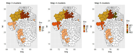
Figure 3.
Maps of the new TPEs determined by the PCA clustering with the number of clusters fixed at three (AE, A1, B), four (AE, A1, B, G), or five (AE1, A1, B, G, AE2).
Table 3.
Descriptive statistics for the newly determined TPEs (A1, AE1, AE2, B, G). AE covers (AE1 and AE2) B+ covers (B and G). The values represent the means over years (1998–2017) with the standard deviation in parenthesis for a specific TPE. Trend values are the linear regression coefficient with standard deviation in parenthesis. Crop model parameters are the average values over districts forming the TPE with standard deviation in parenthesis.
The new TPE characterization showed similarities with the current system for the A1 (North Rajasthan) and B zones that roughly remained the same (Figure 1 and Figure 3). However, the previously defined A zone showed potentially more diversity and can be re-defined into two or three distinct parts (G, AE [AE1, AE2]). Within these, the districts of Gujarat (G) shared more similarities with the B zone and could be seen as a unique entity. Similarly, the eastern part of the original A zone (AE) could be further split into two parts (AE1, AE2).
3.1.1. A-Eastern 1 (AE1) TPE
The proposed AE TPE would encompass the north-eastern districts belonging to A zone of the original classification. This is the only region where pearl millet cultivation area has increased (Figure 4; +0.4 Kha/year between 1998 and 2017). It is also the region with the largest average production (58.6%) and area (2.83 Mha). This region can be further divided into two parts, AE1 covering the western districts (Rajasthan, Haryana), and AE2 the eastern part. The 18 districts of AE1 account for the largest share in production (around 39%) and represented on average 2.09 Mha of cultivated area. The production increase is due to a moderate growth of the cultivated area (+0.3 Kha/year between 1998 and 2017) combined with important yield increase. AE1 districts yield increased on average by 46 kg per ha per year to reach an average of 1694 kg/ha in 2016–2017. This extra yield could be associated with the increased rainfall apparent in the weather data. It was more certainly supported by technological investments in irrigation (+0.6% of irrigated surface per year), fertilization, and possibly new varieties suiting intensified cultivation practices [52].
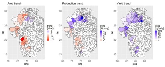
Figure 4.
Maps with the kharif pearl millet cultivated area trend in kilo hectare (Kha) per year, production trend in kilo ton (Kton) per year, and yield trend in kilogram per hectare per year (kg/ha/year) between 1998 and 2017.
3.1.2. A-Eastern 2 (AE2) TPE
The eastern part of AE (AE2, Uttar Pradesh, and Madhya Pradesh) was the only geography where the proportion of pearl millet area compared to other crops (share) has increased (+0.1% per year). In the 12 districts from AE2, the pearl millet production was also characterized by a strong yield increase with an average of 58 kg/ha/year. With an average of 1860 kg/ha between 1998 and 2017, AE2 is the TPE with the highest yield, which makes pearl millet competitive with crops such as maize (1801 kg/ha on average over the same period). This success could be linked to potential moderate rain increase (7 mm/year). With an average of 504 mm of precipitation per year, AE2 is the TPE with the second highest precipitation level. The yield increases experienced in AE2 could also be due to suitable soil (Inceptisol) for pearl millet in terms of soil water content and soil depth. According to the crop model ExM parameter estimation, AE2 had the highest PAWC and deepest soils. AE2 is also a region that benefited from technological investments in terms of irrigation (+0.6% of irrigated surface per year), fertilization (on average 106 kg/ha of N during Kharif), and potentially in terms of improved varieties [52]. Finally, it is interesting to emphasize that AE2 is characterized by the lowest pearl millet price (on average 682 INR/100 kg), which is around 20% less than in A1 (843 INR/100 kg).
3.1.3. The Arid TPE—A1
The TPE characterization recovered most of the original A1 TPE encompassing 11 Western districts of Rajasthan. Between 1998 and 2017, the cultivated area decreased on average by three Kha/year while yield moderately increased (20 kg/ha/year), especially in the southern part (e.g., Jodhpur 34 kg/ha/year), which contributed to the overall production increase (Figure 4). With an average of 2.93 Mha (38.5% of the total area) the A1 TPE remains the most important in terms of surface. The A1 districts experience the most difficult environmental conditions with the lowest average precipitation (249.9 mm) and an inherently low fertility type of sandy soil (Pssament), which has potentially the lowest PAWC and depth. Those constraints probably explain why the A1 yields remain the lowest (499 kg/ha) and this goes together with the low recorded irrigation (4.6% of the area) and fertilization (14.6 kg/ha) levels.
3.1.4. The Transitioning TPE—B
The identified B TPE largely resembles the original B zone, but it has experienced the strongest changes between 1998 and 2017 because the cultivated area and the production have strongly declined (Figure 4). With a yield increase of 14 kg/ha/year, the B TPE had the smallest yield increase. Some districts even experienced a yield decline (e.g., Satara—6.25 kg/ha/year). The main reason explaining this decline might be the competition with alternative crops (Figure S5). Among those, cotton and maize seemed to replace pearl millet in many districts. The decline of pearl millet cultivation can be also linked to a reduction in the resources allocated to this crop (i.e., fertilization, irrigation). For example, the B TPE is the only environment where pearl millet irrigation has declined (−0.1%/year).
3.1.5. The Gujarat TPE—G
The last (G) TPE encompasses seven districts belonging to Gujarat. It shares some characteristics with the B TPE in terms of decreasing area and production trends, as well as with the AE TPE in terms of increasing yield (+51 kg/ha/year) and management practices. Like the B TPE, G has experienced an important decline of both the cultivated area (−4.5 Kha/year) and the production (−1.3 Kton/year). It could be due to surface re-allocation to crops such as cotton or castor bean (Figure S6). In terms of weather, the G TPE shows the highest average of seasonal rain (545.6 mm) and the strongest rainfall variance between seasons. Such a feature could explain a partial re-distribution of the pearl millet production from kharif (rainy season) to the Summer (hot season). In terms of technology, the data show different trends compared to the B TPE because inputs, such as irrigation or fertilization, have increased over 1998–2017. For example, irrigated surface increased on average by 2.2% per year.
3.2. Crop Model Prediction Ability
Table 4 summarizes the crop model yield prediction ability in identified TPEs, overall, over time, and over space. The overall yield prediction ability () was the largest in AE1 (0.54–0.78) and A1 (0.51–0.76) and the lowest in AE2 (0.18–0.61) and B (0.03–0.52). The yield prediction ability over years was also the largest in AE1 (0.32–0.46) and A1 (0.28–0.36) compared to AE2 (−0.06–−0.02) and B (−0.14–0.09). This is potentially due to stronger changes in the pearl millet production over years in B, AE2, and G compared to A1 and AE1. Concerning the location effect, the values were comparatively lower in the B TPE, which suggests more environmental heterogeneity in B while other TPEs are more homogeneous. The observed stronger variability of the system parameter over time compared to space was expected.
Table 4.
Crop model prediction ability over TPEs in three different scenarios (overall, year, location) given two crop model predictions methods (Informed strategy and with estimated ExM parameters). Overall: Pearson correlation between observed and predicted whole time series (1998–2017). Time effect: Pearson correlation between observed yield in future (2008–2017) given parameters estimated in past years (1998–2007). Location effect: Pearson correlation between observed yield in a neighbour district given parameters estimated in another district.
The overall prediction ability obtained with the estimated ExM parameters (0.52–0.78) was greater than the one obtained with the informed strategy (0.03–0.54). However, in the evaluation of the year and location effects, the informed strategy gave more stable results than the estimated ExM parameters except in the B TPE where the informed strategy failed. This result illustrates the advantage of the estimated ExM parameters strategy for locations where information is incomplete, or when the conditions are rapidly changing, such as the B TPE. Except for this specific case, the estimated ExM parameters strategy tends to overfit the data, which limits its capacity of prediction in time and space. The informed strategy seems to offer more stable results.
3.3. Ranges of Crop Model Parameters and Weather Input Influence on Yield
In Table 5, we synthesized the influence of each studied crop model parameter range (Table 2) on the simulated yield in the different TPEs. Overall, the soil water content (PAWC, 0.6–1.3 mm/cm soil) was the parameter with the strongest consistent effect (∈ [0.06–0.1]). Soils with low PAWC (0.6) had significantly reduced yield (600–730 kg/ha) compared to higher PAWC (1.3). The variety also had an overall strong effect on yield. The improved long duration variety (9444) generally had a positive effect on yield (617–938 kg/ha) except in the A1 TPE where the effect was less important (342 kg/ha). In the A1 TPE, the effect of irrigation was the strongest ( = 0.17) with an advantage of 4.75 kg/ha/mm. Irrigation effect was less important in the other TPEs. Compared to soil properties, variety, or irrigation, other tested management practices, such as fertilization, sowing date, or sowing density had less influence on yield.
Table 5.
Crop model parameter influence on grain yield in the new TPEs as the estimated linear regression coefficient (B) and the difference R squared statistics over all simulations.
Concerning the effect of the weather parameters, we noticed that an extra unit of maximum temperature consistently reduced the yield while an extra unit of minimum temperatures increased it. Interestingly, an extra rainfall unit had a positive effect on simulated yield in A1 and AE1 but a negative one in the G, B and AE2 TPEs. Finally, we noticed a strong influence of the model version used with values between 0.03 and 0.18. The updated model tended to overestimate the yield. However, the updated model was better to predict the yield trend in the A1 and AE1 TPEs (Table S2). The parameter relative importance obtained with the alternative metrics (i.e., the relative importance of the sum of squares—Table S3—and the parameter effect range proportion over the yield range—Table S4) were comparable to the results obtained with the difference . However, the relative effect range of the weather (rain, temperature) and irrigation compared to the yield range gave a more important influence to those parameters than the difference and the relative sum of squares.
3.4. Detailed Results about the Estimation ExM Parameters
A novelty of this study was to calibrate the model parameters reflecting the environment and management practices at the district level in order to systematically manage the uncertainity associated with those variables. The prediction abilities of Table 4, gave us a general overview about this strategy. Another evaluation for the estimated ExM parameters approach was to compare the estimated values with real data. The availability of observations on the percentage of irrigated pearl millet and the overall nitrogen fertilization at the district level in the DLD constituted the most direct comparison opportunity. In both cases (Figure 5), we noticed that the observed and estimated ExM parameters had a similar spatial distribution. Irrigation was high in the eastern and Gujarat districts. However, in the B TPE, the estimated ExM parameters overestimated the irrigation level. Concerning fertilization, the recorded usage of nitrogen was consistently higher in the eastern districts, as well as in the B TPE for both observations and estimated ExM parameters. The moderate correlation between estimated ExM parameters and observation of 0.2 and 0.22 for irrigation and fertilization, respectively, showed that the estimated ExM parameters method was only able to approximate general tendencies but failed to predict more extreme observations. The evaluation of the estimated ExM parameters for other variables, such as the soil properties or other management practices, was more difficult because we could not directly compare those to observed values (Figures S7 and S8).
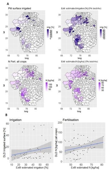
Figure 5.
(A) Comparison of the estimated ExM parameters values for irrigation and fertilization with the average percentage of pearl millet surface under irrigation and the average amount of N fertilization for all crops during kharif according to the DLD (1998–2017) (B) Scatter plots of the estimated ExM parameters and observed district values for irrigation and fertilization.
3.5. Online Application for Results Visualisation
We compiled the article data and results in an R shiny application available on github (https://github.com/vincentgarin/PMapp (accessed on 1 April 2023)). A reduced version of the application without the crop model simulation results is available online (https://agrvis.shinyapps.io/PMapp/ (accessed on 1 April 2023)).
4. Discussion
The main objective of this article was to characterize the Indian pearl millet production regions using novel data sources and state-of-the-art methodologies. This analysis was originally requested by the Indian national and international research institutions to provide a deeper understanding and quantitative base for the optimization of the pearl millet production systems. The revised TPE is still largely based on influential biophysical factors, such as rain pattern, temperature, and the soil characteristics, but provides several novel insights, particularly hinting to the changing climate and socio-economic drivers, which should be further investigated. In the following sections, we will first discuss the implications of important causes of changes like the possible rain pattern increase and the socio-economic aspects driving some of the TPE features. Then, we will discuss the pros and cons for the use of crop models for pearl millet envirotyping.
4.1. Kharif Rain Increase and Transition of Pearl Millet Cultivation to Summer Season
In all TPEs, the Nasapower weather data suggest that the amount of precipitation during kharif has increased between 1998 and 2017. The hypothesis of increasing kharif rains is supported by other sources and is expected to continue [53,54]. Other authors, like Praveen et al. [55], used observed data from the Indian meteorological system and reached the conclusion of a general rain decrease since around 1960. The later reference is, however, supported by less data than [53,54]. Therefore, based on our data and elements of the literature, we will assume the hypothesis of a kharif rain increase between 1998 and 2017 that could continue in the future. Such a change will strongly influence the future strategy for pearl millet systems improvement and should be closely monitored. We suggest that a part of the yield increase observed over the studied period could be due to those extra precipitations.
In other cases however, the potential extra kharif precipitation could directly or indirectly reduce the area allocated to pearl millet cultivation. A first hypothesis would assume a direct negative effect of rain due to an increase in the episodes of high intensity. The extra variability of rain, particularly strong in the G TPE, could result in short and intense rain episodes causing problems of water logging, stem mechanical break, and/or grain mold impacting the crop. Another hypothesis would assume an indirect effect. Indeed, we could also imagine that the extra available water during the traditional pearl millet growing season motivates the farmers to switch to crops that require more water, such as cotton or maize. Such a hypothesis is supported by the important increase area allocated to those crops in the B and G TPEs, which could explain the strong decline of pearl millet in those TPEs (see Section 4.2).
This direct and indirect effect of rain could also partly explain the transfer of the pearl millet cultivation from kharif to Summer season observed in the G TPE and to a lesser extent in AE2 (Figure S9). This transfer was confirmed by several experts and the DLD data. Indeed, in the G TPE, the proportion of area cultivated in Summer has progressively increased to reach more than 50% (Figure S10). However, according to the DLD data, it does not represent a net area transfer between seasons but a larger propensity to cultivate pearl millet during Summer because, even during this season, the total pearl millet area stagnated or even decreased. In the AE2 TPE too, we could observe an increase in the area cultivated in Summer with up to 20 % of the yearly surface around 2009. However, after this year the proportion decreased. Those observations need to be confirmed over longer periods.
4.2. The Essential Role of Socio-Economic Factors in Pearl Millet Cultivation
The average yield increase of 37 kg/ha/year over all districts is similar to Yadav et al. [56] findings, but hides important differences between TPEs (A1: 20 kg/ha/year, AE2: 58 kg/ha/year) that let us suppose some differences in the assimilation of new management practices and varieties. Generally, except in the G TPE, the yield increases were correlated with area trends. In TPE B and G, the decline in the pearl millet cultivated area was strongly correlated with the increased cultivation of crops, such as cotton, maize, or castor bean, having a more structured value chain and a higher profitability [57,58]. Therefore, the overall system dynamic seems to be closely related to socio-economic factors. If this is true, efforts to improve pearl millet production could be in vain if farmers continue to replace pearl millet by higher value crops. The necessity to strengthen the pearl millet value chain by increasing its profitability should, therefore, be a priority. However, such a task seems complicated because government policies, as well as trends such as urbanization and the changes in dietary patterns, are very difficult to influence [59].
Another example of the importance of socio-economic factors was the increase in pearl millet cultivation area in the AE2 TPE while the price per quintal was the lowest. According to regional experts, substantial parts of the AE production (especially AE2) might be exported to A1, where pearl millet is a staple food and market is more important when A1 production is possibly not sufficient (OP Yadav personal communication). The increased prices occurring in A1 (around 20%) can motivate the export between regions. This would represent an example of commercially viable pearl millet value chain, but the hypothesis should be confirmed by further investigations. Generally, our study emphasizes the existence of different socio-economic drivers for pearl millet cultivation in TPE such as A1 that seems more oriented toward subsistence and AE2, which looks more market oriented.
4.3. The Use of Crop Model for Pearl Millet Envirotyping and Its Limitations
A second objective of this article was to test the ability of crop models to reflect the dynamics of the pearl millet production systems in India, which is the basis for future system optimization (e.g., Ronanki et al. [24]), and to incorporate some crop model information into the TPE analysis. Here, we shall emphasize that the APSIM crop models do not simulate important biotic stresses, such as pest and disease attack. For example, it is documented that an important share of pearl millet has suffered from an increasing blast attack [60]. The combined effect of those stresses with the assumption of representing a whole district by a single simulation can explain an important part of the difference between observation and crop model predictions. Despite those, in the A1, AE1, and G TPEs, which represent the large majority of area () and production (), we could obtain prediction abilities between 0.15 and 0.61 (squared correlation for comparison) that were comparable to the values about regional prediction from other studies Chen et al. [61] (0.26–0.42) de Wit et al. [62] (0.24–0.65).
Nevertheless, in regions that potentially experienced rapid changes (B, AE2, and G), the crop model was less effective to capture the production fluctuations. In those TPEs, the prediction ability over the years was strongly reduced, which is likely due to a rapid and large variability in the crop management practices between the seasons. The socio-economic drivers and the potential modification in the rain pattern (see above) could be major drivers of those changes. Therefore, we shall emphasize the interest of combining a large set of data, allowing the joint understanding of biophysical process and socio-economic trends, which seem to have a strong effect on the crop model prediction ability in the future. Reduced prediction abilities in AE2, B, and G could also result from choice of the testing locations to develop the models (Telangana and Rajasthan). The collection of extra data on varieties in AE2, G, and B testing sites during future development would help to improve the crop model prediction ability there.
The evaluation of an updated version of the APSIM model for dynamic tiller simulation was promising. We could show that, despite the general overestimation of the average yield, this new model offered more sensitivity to predict yield trends (+0.18–0.19 correlation) in the A1 and AE1 (core of the pearl millet tract, area, production). Therefore, this model could be used for optimization of the Indian pearl millet system. The crop model sensitivity analysis emphasized the importance of the soil parameters for yield. It supports the conclusion from Carberry et al. [63] that this component should receive extra attention. Finally, the large effect of the variety, especially in AE2, B, and G suggests to further dissect the optimal genotype properties to enhance pearl millet production in those TPEs.
One of the novelties presented in this article was the use of extended simulations to estimate ExM parameters. We showed that this strategy could help to estimate parameters with large influence on yield like soil water content or irrigation, but its capacity to infer less influential parameters, such as the sowing date, was weak. Generally, the ExM parameters estimation tended to determine values that overfit the observed data. Nevertheless, the estimation of ExM parameters could be useful in situations with low levels of information.
5. Conclusions
In this section, we summarize the main characteristics of each TPE.
A1 (2.9 Mha, 1.4 Mton, 499 kg/ha): This TPE is characterized by harsh agronomic conditions due to low precipitation, high temperature, and potentially poor soils (sandy soils, low water content). This scarcity largely explains the reduced number of alternatives to pearl millet in A1, which is an important reason for its stability there. Potential reduced benefits could explain the low level of input (irrigation, fertilization) and the limited effect of improved varieties observed in the A1 TPE. Our data revealed that a proportion of pearl millet might be imported from AE but further investigation is needed to confirm this hypothesis. Increasing the local production to meet this demand could be a driver for pearl millet cultivation in A1. With 8 testing sites out of 76 in the All India Coordinated Research Project (AICRP; Figure 1B), the A1 TPE is under-represented. Resources from sites falling in none of the TPEs (17/76), from the B TPE (17/76) or the G TPE (14/76) should be re-allocated to A1. Districts (Rajasthan): Barmer, Bikaner, Churu, Hanumangarh, Jaisalmer, Jalore, Jodhpur, Nagaur, Pali.
AE1 (2.1 Mha, 2.8 Mton, 1397 kg/ha): This TPE is the area where most of the pearl millet was produced between 1998 and 2017 (around 39% of the total production). The increase in production is due to a moderate growth of the cultivated area together with high yield increase that appeared to be associated with good soil properties, technological investments (irrigation, fertilization, improved varieties), and a hypothetical rain increase. We recommend to increase the attention on this TPE, for example by allocating more testing sites there, especially in AE1 southeast part (Figure 1B). Districts (Rajasthan): Ajmer, Alwar, Bharatpur, Dausa, Jaipur, Jhunjhunu, Karauli, Sawai Madhopur, Sikar, Tonk; (Haryana): Bhiwani, Gurgaon, Hisar, Jhajjar, Jind, Mahendragarh, Rewari; (Uttar Pradesh): Mathura.
AE2 (0.7 Mha, 1.37 Mton, 1859 kg/ha): AE2 is the only TPE where the fraction of area under pearl millet cultivation increased between 1998 and 2017. This success could be linked to suitable soil type (higher water content and depth), and a potential moderate increase in rain. AE2 is a region where pearl millet production benefited from technological investment (fertilization, irrigation, possibly adoption of new hybrid cultivars), which made pearl millet competitive with respect to other crops such as maize. The lowest market prices obtained in AE2 support the hypothesis of an exportation of surplus into the A1 TPE. With 6 testing sites out of 76, this TPE is the least represented among the AICRP testing sites (Figure 1B). It would be strategic to increase the testing sites coverage to better understand the reasons of AE2 success and the way the pearl millet economy functions in this region. Districts (Uttar Pradesh): Agra, Aligarh, Auraiya, Budaun, Etah, Etawah, Firozabad, Kasganj, Sambhal; (Madhya Pradesh): Bhind, Morena; (Rajasthan): Dholpur.
B (1.4 Mha, 1.1 Mton, 788 kg/ha): The B TPE is characterized by the largest decline of area under pearl millet cultivation. The presence of many alternatives, such as cotton and maize, with more profitable value chains might explain the transition from pearl millet to other crops. This declining interest translated in a low level of technological investment and resulted in very limited yield increases. Therefore, we recommend to investigate the reasons for abandoning pearl millet cultivation in this TPE. Districts (Maharashtra): Ahmednagar, Aurangabad, Beed, Dhule, Jalgaon, Jalna, Nashik, Pune, Sangli, Satara; (Karnataka): Bagalkot, Bijapur, Gulbarga, Koppal, Raichur; (Uttar Pradesh): Allahabad.
G (0.4 Mha, 0.5 Mton, 1208 kg/ha): In Gujarat, the pearl millet production sharply decreased, probably because of the availability of more profitable crops, such as cotton or castor beans. The data suggest that a part of the kharif pearl millet production has been transferred to Summer. This transfer is potentially due to an increase in the rain volume and variability during kharif. Despite a relatively high investment in technology (irrigation, fertilization) and high yield, the reduction in the pearl millet cultivated area was not compensated by the extra yield. The G TPE can be used as a testing site to investigate the influence of rain pattern on pearl millet cultivation, especially the question of potential cultivation transfer between the seasons. Districts (Gujarat): Banas Kantha, Bhavnagar, Kachchh, Kheda, Mahesana, Patan.
Supplementary Materials
The following supporting information can be downloaded at: https://www.mdpi.com/article/10.3390/agronomy13061607/s1, Figure S1: Map of the rain pattern; Figure S2: Map of the temperature pattern; Figure S3: Map of the majority soil type in the pearl millet tract; Figure S4: Crop model ExM parameter calibration illustration; Figure S5: B zone area share, area trend and production compared to other crops; Figure S6: G zone area and production trend compared to other crops; Figure S7: Comparison between observed data and ExM parameters values - soil parameters; Figure S8: Comparison between observed data and ExM parameters values - management parameters; Figure S9: Pearl millet area trend over seasons in the AE2 zone; Figure S10: Pearl millet area trend over seasons in the G zone; Table S1: Reference selection of crop model parameter following the ’informed strategy’; Table S2: Influence of the crop model parameters on the crop model prediction ability; Table S3: Influence of the crop model parameters on predicted yield - relative sum of square; Table S4: Influence of the crop model parameters on predicted yield - relative estimated effect;
Author Contributions
Conceptualization, V.G. and J.K.; methodology, V.G., S.C. and J.K.; data collection, T.M., S.K., M.D., J.K. and S.C.; data curation, V.G.; formal analysis, V.G. and A.H.; writing—original draft preparation, V.G., S.C. and J.K.; writing—review and editing, V.G., S.C., J.K., T.S.C. and S.K.G.; supervision, J.K., T.S.C. and S.K.G.; funding acquisition, V.G., J.K., T.S.C. and S.K.G. All authors have read and agreed to the published version of the manuscript.
Funding
This research article is part of a joint initiative between ICRISAT and ICAR to design the strategies for sustainable improvement of pearl millet cultivation in India. It benefited from the ICAR-ICRISAT collaboration funding and from the Crops to End Hunger initiative. This research was also supported by the Swiss National Science Foundation that subsidised Dr. Vincent Garin (Postoc.Mobility grant no: P500PB_203030). Dr. Jana Kholovà work was financed by an internal grant agency of the Faculty of Economics and Management from the Czech University of Life Sciences Prague (Grant Life Sciences 4.0 Plus no. 2022B0006). Sivasakthi Kaliamoorthy and Tharanya Murugesan were supported by the Global Challenge Research Fund (GCRF)/Biotechnology and Biological Sciences Research Council (BBSRC)-funded project Transforming India’s Green Revolution by Research and Empowerment for Sustainable food Supplies (TIGR2ESS; BB/P027970/1; 2018–22).
Data Availability Statement
All data and results can be accessed at the following github repository: https://github.com/vincentgarin/PMapp (accessed on 1 April 2023).
Acknowledgments
We thank Greg McLean, Erik van Oosterom and Graeme Hammer for their help with the implementation of the new pearl millet model. We also thank Janila Pasupuleti, Ashok Kumar Are from ICRISAT, O.P. Yadav from ICAR-CAZRI, Rajendra Singh Mahala from SeedWorks International Private Limited, Yogendra Verma from Kaveri Seed Company Limited and Sanjana P Reddy from ICAR-IIMR for the discussion about the article content.
Conflicts of Interest
The authors declare no conflict of interest.
Abbreviations
The following abbreviations are used in this manuscript:
| MDPI | Multidisciplinary Digital Publishing Institute |
| DOAJ | Directory of open access journals |
| TLA | Three letter acronym |
| LD | Linear dichroism |
References
- Jukanti, A.; Gowda, C.L.; Rai, K.; Manga, V.; Bhatt, R. Crops that feed the world 11. Pearl Millet (Pennisetum glaucum L.): An important source of food security, nutrition and health in the arid and semi-arid tropics. Food Secur. 2016, 8, 307–329. [Google Scholar] [CrossRef]
- Yadav, O.P.; Rai, K.N. Genetic Improvement of Pearl Millet in India. Agric. Res. 2013, 2, 275–292. [Google Scholar] [CrossRef]
- Yadav, O.; Rai, K.; Rajpurohit, B.; Hash, C.; Mahala, R.; Gupta, S.; Shetty, H.; Bishnoi, H.; Rathore, M.; Kumar, A.; et al. Twenty-Five Years of Pearl Millet Improvement in India; ICAR: New Delhi, India, 2012. [Google Scholar]
- Nedumaran, S.; Bantilan, M.; Gupta, S.; Irshad, A.; Davis, J. Potential Welfare Benefit of Millets Improvement Research at ICRISAT: Multi Country-Economic Surplus Model Approach; Socioeconomics Discussion Paper Series Number 15; ICRISAT: Hyderabad, India, 2014. [Google Scholar]
- Nagaraj, N.; Basavaraj, G.; Rao, P.P.; Bantilan, C.; Haldar, S. Sorghum and pearl millet economy of India: Future outlook and options. Econ. Political Wkly. 2013, 28, 74–81. [Google Scholar]
- Rao, C.R.; Raju, B.; Rao, A.; Reddy, D.Y.; Meghana, Y.; Swapna, N.; Chary, G.R. Yield vulnerability of sorghum and pearl millet to climate change in India. Indian J. Agric. Econ. 2019, 74, 350–362. [Google Scholar]
- Hammer, G.L.; McLean, G.; Chapman, S.; Zheng, B.; Doherty, A.; Harrison, M.T.; van Oosterom, E.; Jordan, D. Crop design for specific adaptation in variable dryland production environments. Crop Pasture Sci. 2014, 65, 614–626. [Google Scholar] [CrossRef]
- Harrison, M.T.; Tardieu, F.; Dong, Z.; Messina, C.D.; Hammer, G.L. Characterizing drought stress and trait influence on maize yield under current and future conditions. Glob. Change Biol. 2014, 20, 867–878. [Google Scholar] [CrossRef] [PubMed]
- Messina, C.D.; Cooper, M.; Reynolds, M.; Hammer, G.L. Crop science: A foundation for advancing predictive agriculture. Crop Sci. 2020, 60, 544–546. [Google Scholar] [CrossRef]
- Chapman, S.; Cooper, M.; Butler, D.; Henzell, R. Genotype by environment interactions affecting grain sorghum. I. Characteristics that confound interpretation of hybrid yield. Aust. J. Agric. Res. 2000, 51, 197–208. [Google Scholar] [CrossRef]
- Chenu, K.; Deihimfard, R.; Chapman, S.C. Large-scale characterization of drought pattern: A continent-wide modelling approach applied to the Australian wheatbelt—Spatial and temporal trends. New Phytol. 2013, 198, 801–820. [Google Scholar] [CrossRef] [PubMed]
- Casadebaig, P.; Zheng, B.; Chapman, S.; Huth, N.; Faivre, R.; Chenu, K. Assessment of the potential impacts of wheat plant traits across environments by combining crop modeling and global sensitivity analysis. PLoS ONE 2016, 11, e0146385. [Google Scholar] [CrossRef]
- Hajjarpoor, A.; Kholová, J.; Pasupuleti, J.; Soltani, A.; Burridge, J.; Degala, S.B.; Gattu, S.; Murali, T.; Garin, V.; Radhakrishnan, T.; et al. Environmental characterization and yield gap analysis to tackle genotype-by-environment-by-management interactions and map region-specific agronomic and breeding targets in groundnut. Field Crops Res. 2021, 267, 108160. [Google Scholar] [CrossRef]
- Rahimi-Moghaddam, S.; Deihimfard, R.; Nazari, M.R.; Mohammadi-Ahmadmahmoudi, E.; Chenu, K. Understanding wheat growth and the seasonal climatic characteristics of major drought patterns occurring in cold dryland environments from Iran. Eur. J. Agron. 2023, 145, 126772. [Google Scholar] [CrossRef]
- Braun, H.J.; Rajaram, S.; Ginkel, M. CIMMYT’s approach to breeding for wide adaptation. In Adaptation in Plant Breeding; Springer: Heidelberg, Germany, 1997; pp. 197–205. [Google Scholar]
- Chauhan, Y.; Rachaputi, R.C. Defining agro-ecological regions for field crops in variable target production environments: A case study on mungbean in the northern grains region of Australia. Agric. For. Meteorol. 2014, 194, 207–217. [Google Scholar] [CrossRef]
- Ghosh, S. Agro-Climatic Zone Specific Research: Indian Perspective under NARP-ICAR; ICAR: New Delhi, India, 1991; pp. 1–539. [Google Scholar]
- Packwood, A.; Virk, D.; Witcombe, J. Trial testing sites in the All India Coordinated Projects—How well do they represent agro-ecological zones and farmers’ fields. In Seeds of Choice: Making the Most of New Varieties for Small Farmers; Intermediate Technology Publications: Lucknow, India, 1998; pp. 7–26. [Google Scholar]
- Gupta, S.; Rathore, A.; Yadav, O.; Rai, K.; Khairwal, I.; Rajpurohit, B.; Das, R.R. Identifying mega-environments and essential test locations for pearl millet cultivar selection in India. Crop Sci. 2013, 53, 2444–2453. [Google Scholar] [CrossRef]
- Kholovà, J.; Adam, M.; Diancoumba, M.; Hammer, G.; Hajjarpoor, A.; Chenu, K.; Jarolímek, J. Sorghum: General Crop-Modelling Tools Guiding Principles and Use of Crop Models in Support of Crop Improvement Programs in Developing Countries. In Sorghum in the 21st Century: Food–Fodder–Feed–Fuel for a Rapidly Changing World; Springer: Heidelberg, Germany, 2020; pp. 189–207. [Google Scholar]
- Kholovà, J.; Hajjarpoor, A.; Garin, V.; Nelson, W.; Diacoumba, M.; Messina, C.D.; Hammer, G.L.; Xu, Y.; Urban, M.O.; Jarolimek, J. The role of crop growth models in crop improvement: Integrating phenomics, envirotyping and genomic prediction. In Advances in Plant Phenotyping for More Sustainable Crop Production; Burleigh Dodds Science Publishing: Cambridge, UK, 2022; pp. 263–282. [Google Scholar]
- Messina, C.; Hammer, G.; Dong, Z.; Podlich, D.; Cooper, M. Modelling crop improvement in a G× E× M framework via gene-trait-phenotype relationships. In Crop Physiology: Interfacing with Genetic Improvement and Agronomy; Elsevier: Amsterdam, The Netherlands, 2009; pp. 235–265. [Google Scholar]
- Tardieu, F.; Reymond, M.; Muller, B.; Granier, C.; Simonneau, T.; Sadok, W.; Welcker, C. Linking physiological and genetic analyses of the control of leaf growth under changing environmental conditions. Aust. J. Agric. Res. 2005, 56, 937–946. [Google Scholar] [CrossRef]
- Ronanki, S.; Pavlík, J.; Masner, J.; Jarolímek, J.; Stočes, M.; Subhash, D.; Talwar, H.S.; Tonapi, V.A.; Srikanth, M.; Baddam, R.; et al. An APSIM-powered framework for post-rainy sorghum-system design in India. Field Crops Res. 2022, 277, 108422. [Google Scholar] [CrossRef]
- Alam, M.M.; Hammer, G.L.; Van Oosterom, E.J.; Cruickshank, A.W.; Hunt, C.H.; Jordan, D.R. A physiological framework to explain genetic and environmental regulation of tillering in sorghum. New Phytol. 2014, 203, 155–167. [Google Scholar] [CrossRef]
- Alam, M.M.; van Oosterom, E.J.; Cruickshank, A.W.; Jordan, D.R.; Hammer, G.L. Predicting tillering of diverse sorghum germplasm across environments. Crop Sci. 2017, 57, 78–87. [Google Scholar] [CrossRef]
- Van Oosterom, E.; Carberry, P.; Hargreaves, J.; O’leary, G. Simulating growth, development, and yield of tillering pearl millet: II. Simulation of canopy development. Field Crops Res. 2001, 72, 67–91. [Google Scholar] [CrossRef]
- Sultan, B.; Roudier, P.; Quirion, P.; Alhassane, A.; Muller, B.; Dingkuhn, M.; Ciais, P.; Guimberteau, M.; Traore, S.; Baron, C. Assessing climate change impacts on sorghum and millet yields in the Sudanian and Sahelian savannas of West Africa. Environ. Res. Lett. 2013, 8, 014040. [Google Scholar] [CrossRef]
- Singh, P.; Boote, K.; Kadiyala, M.; Nedumaran, S.; Gupta, S.; Srinivas, K.; Bantilan, M. An assessment of yield gains under climate change due to genetic modification of pearl millet. Sci. Total Environ. 2017, 601, 1226–1237. [Google Scholar] [CrossRef] [PubMed]
- Sparks, A. Nasapower: NASA-POWER Data from R. R Package Version 4.0.0; Foundation for Statistical Computing: Vienna, Austria, 2021. [Google Scholar]
- Laryea, K.B. Distribution of Soils in Production Systems in India; ICRISAT: Patancheru, India, 1998. [Google Scholar]
- Hajjarpoor, A.; Vadez, V.; Soltani, A.; Gaur, P.; Whitbread, A.; Babu, D.S.; Gumma, M.K.; Diancoumba, M.; Kholová, J. Characterization of the main chickpea cropping systems in India using a yield gap analysis approach. Field Crops Res. 2018, 223, 93–104. [Google Scholar] [CrossRef]
- Miguez, F. Apsimx: Inspect, Read, Edit and Run ‘APSIM’ “Next Generation” and ‘APSIM’ Classic, R Package Version 2.3.1; Foundation for Statistical Computing: Vienna, Austria, 2022.
- Hartigan, J.A.; Wong, M.A. Algorithm AS 136: A k-means clustering algorithm. J. R. Stat. Society. Ser. C Appl. Stat. 1979, 28, 100–108. [Google Scholar] [CrossRef]
- Holzworth, D.P.; Huth, N.I.; deVoil, P.G.; Zurcher, E.J.; Herrmann, N.I.; McLean, G.; Chenu, K.; van Oosterom, E.J.; Snow, V.; Murphy, C.; et al. APSIM—Evolution towards a new generation of agricultural systems simulation. Environ. Model. Softw. 2014, 62, 327–350. [Google Scholar] [CrossRef]
- Van Oosterom, E.; Carberry, P.; O’leary, G. Simulating growth, development, and yield of tillering pearl millet: I. Leaf area profiles on main shoots and tillers. Field Crops Res. 2001, 72, 51–66. [Google Scholar] [CrossRef]
- Van Oosterom, E.; O’leary, G.; Carberry, P.; Craufurd, P. Simulating growth, development, and yield of tillering pearl millet. III. Biomass accumulation and partitioning. Field Crops Res. 2002, 79, 85–106. [Google Scholar] [CrossRef]
- Kim, H.K.; Van Oosterom, E.; Dingkuhn, M.; Luquet, D.; Hammer, G. Regulation of tillering in sorghum: Environmental effects. Ann. Bot. 2010, 106, 57–67. [Google Scholar] [CrossRef]
- Kim, H.K.; Luquet, D.; van Oosterom, E.; Dingkuhn, M.; Hammer, G. Regulation of tillering in sorghum: Genotypic effects. Ann. Bot. 2010, 106, 69–78. [Google Scholar] [CrossRef] [PubMed]
- Garin, V.; van Oosterom, E.; McLean, G.; Hammer, G.; Murugesan, T.; Kaliamoorthy, S.; Diancumba, M.; Hajjarpoor, A.; Kholovà, J. New algorithm for pearl millet modelling in APSIM allowing a mechanistic simulation of tillers. bioRxiv 2023. [Google Scholar] [CrossRef]
- Wallach, D.; Palosuo, T.; Thorburn, P.; Hochman, Z.; Gourdain, E.; Andrianasolo, F.; Asseng, S.; Basso, B.; Buis, S.; Crout, N.; et al. The chaos in calibrating crop models: Lessons learned from a multi-model calibration exercise. Environ. Model. Softw. 2021, 145, 105206. [Google Scholar] [CrossRef]
- Wallach, D.; Makowski, D.; Jones, J.W.; Brun, F. Working with Dynamic Crop Models: Methods, Tools and Examples for Agriculture and Environment; Academic Press: Cambridge, MA, USA, 2018. [Google Scholar]
- Varella, H.; Guérif, M.; Buis, S.; Beaudoin, N. Soil properties estimation by inversion of a crop model and observations on crops improves the prediction of agro-environmental variables. Eur. J. Agron. 2010, 33, 139–147. [Google Scholar] [CrossRef]
- Therond, O.; Hengsdijk, H.; Casellas, E.; Wallach, D.; Adam, M.; Belhouchette, H.; Oomen, R.; Russell, G.; Ewert, F.; Bergez, J.E.; et al. Using a cropping system model at regional scale: Low-data approaches for crop management information and model calibration. Agric. Ecosyst. Environ. 2011, 142, 85–94. [Google Scholar] [CrossRef]
- Huang, J.; Gómez-Dans, J.L.; Huang, H.; Ma, H.; Wu, Q.; Lewis, P.E.; Liang, S.; Chen, Z.; Xue, J.H.; Wu, Y.; et al. Assimilation of remote sensing into crop growth models: Current status and perspectives. Agric. For. Meteorol. 2019, 276, 107609. [Google Scholar] [CrossRef]
- Koo, J.; Dimes, J. HC27 generic soil profile database; IFPRI: Washington, DC, USA, 2013. [Google Scholar]
- Burk, L.; Dalgliesh, N. Estimating Plant Available Water Capacity; Grains Research and Development Corporation: Barton, Australia, 2013. [Google Scholar]
- Rana, K.; Kumar, D.; Bana, R. Agronomic research on pearlmillet (Pennisetum glaucum L.). Indian J. Agron. 2012, 57, 45–51. [Google Scholar]
- Bidinger, F.; Sharma, M.; Yadav, O. Performance of landraces and hybrids of pearl millet [Pennisetum glaucum (L.) R. Br.] under good management in the arid zone. Indian J. Genet. Plant Breed. 2008, 68, 145–148. [Google Scholar]
- Asare-Marfo, D.; Birol, E.; Roy, D. Investigating Farmers’ Choice of Pearl Millet Varieties in India to Inform Targeted Biofortification Interventions: Modalities of Multi-stakeholder Data Collection; University of Cambridge, Environmental Economy and Policy Research Group: Cambridge, UK, 2010. [Google Scholar]
- Munasib, A.; Roy, D.; Birol, E. Networks and low adoption of hybrid technology: The case of pearl millet in Rajasthan, India. Gates Open Res 2019, 3, 1133. [Google Scholar]
- Rao, N.; Rao, K.; Gupta, S.; Mazvimavi, K.; Charyulu, D.; Nagaraj, N.; Singh, R.; Singh, S.; Singh, S. Impact of ICRISAT Pearl Millet Hybrid Parents Research Consortium (PMHPRC) on the Livelihoods of Farmers in India; Research Report; International Crops Research Institute for the Semi-Arid Tropics ICRISAT: Patancheru, India, 2018. [Google Scholar]
- Jin, Q.; Wang, C. A revival of Indian summer monsoon rainfall since 2002. Nat. Clim. Change 2017, 7, 587–594. [Google Scholar] [CrossRef]
- Katzenberger, A.; Schewe, J.; Pongratz, J.; Levermann, A. Robust increase of Indian monsoon rainfall and its variability under future warming in CMIP6 models. Earth Syst. Dyn. 2021, 12, 367–386. [Google Scholar] [CrossRef]
- Praveen, B.; Talukdar, S.; Mahato, S.; Mondal, J.; Sharma, P.; Islam, A.R.M.; Rahman, A. Analyzing trend and forecasting of rainfall changes in India using non-parametrical and machine learning approaches. Sci. Rep. 2020, 10, 10342. [Google Scholar] [CrossRef]
- Yadav, O.P.; Gupta, S.; Govindaraj, M.; Sharma, R.; Varshney, R.K.; Srivastava, R.K.; Rathore, A.; Mahala, R.S. Genetic gains in pearl millet in India: Insights into historic breeding strategies and future perspective. Front. Plant Sci. 2021, 12, 396. [Google Scholar] [CrossRef]
- Blaise, D.; Kranthi, K. Cotton production in India. Cotton Prod. 2019, 193–215. [Google Scholar]
- Hellin, J.; Erenstein, O. Maize-poultry value chains in India: Implications for research and development. J. New Seeds 2009, 10, 245–263. [Google Scholar] [CrossRef]
- Basavaraj, G.; Rao, P.P.; Bhagavatula, S.; Ahmed, W. Availability and utilization of pearl millet in India. SAT Ejournal 2010, 8, 1–6. [Google Scholar]
- Singh, S.; Sharma, R.; Pushpavathi, B.; Gupta, S.K.; Durgarani, C.V.; Raj, C. Inheritance and allelic relationship among gene (s) for blast resistance in pearl millet [Pennisetum glaucum (L.) R. Br.]. Plant Breed. 2018, 137, 573–584. [Google Scholar] [CrossRef]
- Chen, Y.; Zhang, Z.; Tao, F. Improving regional winter wheat yield estimation through assimilation of phenology and leaf area index from remote sensing data. Eur. J. Agron. 2018, 101, 163–173. [Google Scholar] [CrossRef]
- De Wit, A.; Duveiller, G.; Defourny, P. Estimating regional winter wheat yield with WOFOST through the assimilation of green area index retrieved from MODIS observations. Agric. For. Meteorol. 2012, 164, 39–52. [Google Scholar] [CrossRef]
- Carberry, P.; Hochman, Z.; Hunt, J.; Dalgliesh, N.; McCown, R.; Whish, J.; Robertson, M.; Foale, M.; Poulton, P.; Van Rees, H. Re-inventing model-based decision support with Australian dryland farmers. 3. Relevance of APSIM to commercial crops. Crop Pasture Sci. 2009, 60, 1044–1056. [Google Scholar] [CrossRef]
Disclaimer/Publisher’s Note: The statements, opinions and data contained in all publications are solely those of the individual author(s) and contributor(s) and not of MDPI and/or the editor(s). MDPI and/or the editor(s) disclaim responsibility for any injury to people or property resulting from any ideas, methods, instructions or products referred to in the content. |
© 2023 by the authors. Licensee MDPI, Basel, Switzerland. This article is an open access article distributed under the terms and conditions of the Creative Commons Attribution (CC BY) license (https://creativecommons.org/licenses/by/4.0/).