Article

Farm Household Typology Based on Soil Quality and Influenced by Socio-Economic Characteristics and Fertility Management Practices in Eastern Kenya

1
Department of Agricultural Sciences, School of Agriculture and Biotechnology, Karatina University, Karatina P.O. Box 1957-10101, Kenya
2
Department of Soil Science, Institute of Environmental Sciences, Hungarian University of Agriculture and Life Sciences, Páter Károly u. 1, H-2100 Gödöllő, Hungary
3
Agrotechnology National Laboratory, Hungarian University of Agriculture and Life Sciences, Páter Károly u. 1, H-2100 Gödöllő, Hungary
4
Department of Nature Conservation and Landscape Management, Institute for Wildlife Management and Nature Conservation, Hungarian University of Agriculture and Life Sciences, Páter Károly u. 1, H-2100 Gödöllő, Hungary
*
Author to whom correspondence should be addressed.
Agronomy 2023, 13(4), 1101; https://doi.org/10.3390/agronomy13041101
Submission received: 2 March 2023 / Revised: 27 March 2023 / Accepted: 6 April 2023 / Published: 12 April 2023

Abstract

:
The smallholder farming systems in Sub-Saharan Africa (SSA) are highly diverse and heterogeneous in terms of biophysical and socio-economic characteristics. This study was conducted in upper Eastern Kenya (UEK) to categorize farm households and determine the influence of socio-economic characteristics (SeC) and soil fertility management practices (SFMP) on soil fertility across farms. Conditioned Latin hypercube sampling (cLHS) was performed to determine 69 soil sampling sites within Meru and Tharaka Nithi counties. From each household (whose field soil sample was obtained), data relating to resource endowment and soil fertility management were collected through a household questionnaire survey. Standard laboratory procedures were used to analyse soil samples. Data reduction was performed using categorical principal component analysis (CATPCA) (for SeC and SFMP) and standard principal component analysis (PCA) (for soil properties). Two-step cluster analysis identified three distinct farm categories or farm types (FT), namely, low fertility farms (FT1), moderately fertile farms (FT2), and fertile farms (FT3). The correlation of clusters against soil properties was significant across pH, soil organic carbon (SOC), cation exchange capacity (CEC), available P, plant available K, and exchangeable bases. FT1 had low SOC, pH, CEC and available P (soil characteristics), low usage of fertilizer and manure (soil fertility management), and smaller household size, lower income, and smaller farm size (socio-economic). FT2 had lower SOC (compared to FT3) and available P. In terms of soil fertility management, FT2 had higher cases of fallowing and composting with moderate fertilizer usage. Households in this category had moderate income, family size, and land size (socio-economic). FT3 had relatively high SOC, pH, CEC, and mineral nutrients. This farm type was characterized by high fertilizer use (soil fertility management) as well as larger household size, higher income, and larger farm size (socio-economic). The results indicate the importance of nutrient management in enhancing soil quality. Delineation and characterization of farms based on the various parameters including resource endowment reveal imbalanced farm resource flows, suggesting a need for locally tailored interventions suited for location-specific conditions to facilitate improved targeting of soil fertility-enhancing technologies and sustainable crop production regimes. While fertilizer is one of the most critical inputs for enhancing agricultural production, it is a major contributor to nitrous oxide emissions from agriculture and can have negative environmental effects on soil biota and water sources. Farmers’ knowledge on the use of fertilizer is thus necessary in developing strategies (such as integrated approach) to promote its efficient use and minimize its detrimental impacts.

1. Introduction

The smallholder farming systems in much of Sub-Saharan Africa (SSA) is characterized by a wide diversity of farming households and heterogeneity for both biophysical and socio-economic conditions [1,2]. Over time, these differences in drivers and in farm features lead to temporal and spatial variability between and within farming systems. The widespread variability in soil fertility that characterizes most of the African smallholder farming systems is a product of both short and long-term processes linked with land use (including soil fertility management practices), operating over soils with inherently diverse quality [3]. Soil quality can be defined as “fitness for use” or the capacity of a soil to function for a given land use. A high soil quality, in an agricultural context, implies a highly productive soil with minimal levels of degradation [4].
The heterogeneity of farm systems is created by a host of biophysical (including climate, soil fertility, slope etc.) and socio-economic (including farm preferences, prices, production objectives etc.) factors [5]. Several researchers have examined factors such as farm resources, cash, labor, infrastructure, markets, soil fertility management practices [3], and technological level [6]. The selection of factors that define farm differences varies greatly from study to study and is governed by the objectives of research.
Moreover, land degradation is a common phenomenon in many parts of the world, particularly in the developing countries, including Kenya. Consequently, there has been consistent decline in farm productivity due to deteriorating soil fertility [7]. Decline in soil quality and its manifestation (including increased erosion, reduced SOC) translates to decline in environmental quality, thus jeopardizing the livelihoods of a significant proportion of the world population [8]. Sustainable soil fertility and land management are therefore of global urgency [9].
Soil fertility management practices, resource availability, and the pattern of resource allocation to different activities are highly influenced by household endowment, priorities, and household production objectives. Thus, the intensity of nutrient use varies between farms with different resource capabilities and production orientation, which can lead to variation in soil fertility and crop productivity at the farm level [10]. The status and variability of soil fertility within smallholder farms are likely to vary between households of different socio-economic status, or between those pursuing different farm objectives (for example market orientation against subsistence orientation). Within individual farms, resource limitation forces farmers to preferentially allocate available labor and nutrient resources to certain fields, which contributes to the creation of spatial soil variability [1].
Meru and Tharaka Nithi Counties in Kenya are characterized by intensely managed fields and wide variability in the agricultural drivers, which have resulted into different land uses that range from strongly market-oriented small-holder coffee, tea and dairy systems, through semi-commercial cereal/legume-based systems, to subsistence-oriented systems based on staple food crops [11]. In general, continuous-intensive cropping with few or no nutrient inputs coupled with removal of crop residues from the fields has led to a variable fertility status of the soils [12], and the impact of household resource endowment on soil fertility management practices has been documented [13]. Important knowledge gaps need to be explored on the relationship between household characteristics, soil-crop management practices, and soil fertility in increasingly changing farming systems. This paper aims to explore the hypothesis that soil quality is influenced by farmers’ soil fertility management practices and socio-economic characteristics. First, farm households are typified based on soil quality, followed by characterization of the identified typologies based on the socio-economic characteristics (SeC) and soil fertility management practices (SFMP).

2. Materials and Methods

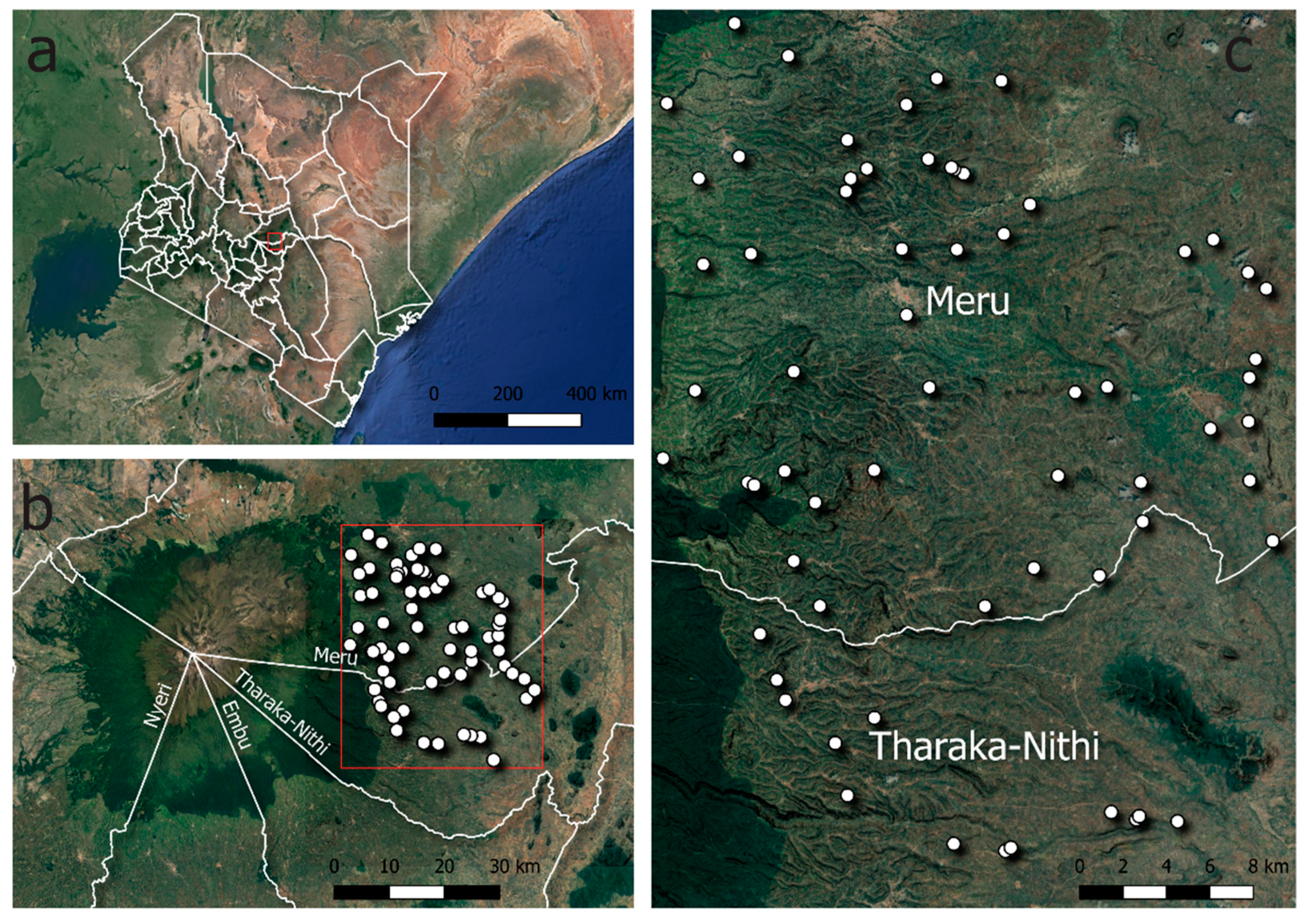
2.1. Study Area Description

The study was conducted in two counties in the upper Eastern Kenya region, namely Meru and Tharaka Nithi (Figure 1). Tharaka Nithi County is found in the semi-arid area of Eastern Kenya, approximately 175 km northeast of Nairobi. It lies on the foothills of Mount Kenya, covering approximately 2638.8 km2. The county borders Meru County to the North, Kitui County to the east and southeast and Embu County to the south. According to data from the Kenya National Bureau of Statistics, the county has a total population of 393,177 inhabitants [14] and a density of 153 persons/km2. Tharaka Nithi County is located in the upper midland zone two (UM2) and upper midland zone three (UM3) agro-ecological zones (AEZ) on the eastern slopes of Mt. Kenya. Upper midland zone 2 is the main coffee zone while the UM3 is the marginal coffee zone. The area lies at an altitude of 1500 m and has an annual mean temperature of 20 °C and a bimodal rainfall pattern totaling 1200 to 1400 mm [15]. The area is a predominantly maize (Zea mays L.) growing zone, as an annual crop, with small land holdings averaging two acres.
Meru County shares borders with Laikipia County to the west, Nyeri County to the southwest, Tharaka Nithi County to the east and Isiolo County to the north. It lies within latitudes 003′45′′ N and 002′30′′, and longitudes 370 and 380 E on the eastern slopes of Mount Kenya. Meru County covers a range of altitudes between 500 m and 5199 m above sea level. The county has a total area of 6936.2 km2 while forest cover is 1776.1 km2 and comprises about twenty different sub-agro-ecozones. The population is approximately 1545,714 [14], while its population density is 221 persons/km2. The predominant soil types in both counties are Nitisols, Ferralsols, Leptosols, Vertisols, Acrisols and Phaeozems [15,16].
The justification for the selection of the study sites was due to the wide range of socio-economic and biophysical conditions, which are typical of highlands, midlands, and lowlands where both mixed farming and agro-pastoralism are practiced by farmers. About 60% of this area has high-to-medium agricultural potential with cash crop and livestock farming as the main sources of livelihood.

2.2. Data Collection Procedures

2.2.1. Soil Sampling

Sampling sites were determined based on conditioned Latin Hypercube Sampling (cLHS). This sampling procedure makes use of the available information on topography, land cover, vegetation, soil types, and land cover/land use to produce optimized sampling stratification, and thus is the most preferred soil sampling design [17]. In addition, cLHS ensures that sampling is implemented in a cost-effective manner by incorporating operational constraints in the model (e.g., by avoiding the selection of hardly accessible, protected, even dangerous areas) [18]. Samples were obtained from 69 fields at surface depth (0–20 cm). The samples were taken within a 3-week sampling campaign period in January 2019. One field per farm household was sampled. The sampling sites represent rainfed agricultural areas with farming that is dominated by smallholder farmers and very diverse agricultural production. The collected samples were delivered to the Hungarian University of Agriculture and Life Sciences (MATE) laboratory for further processing and analysis.

2.2.2. Laboratory Soil Analysis

In the laboratory, the soil samples were air-dried by spreading each sample on a paper at room temperature [19]. The samples were then carefully pounded using a pestle and mortar and passed through a 2 mm mesh sieve.
Soil organic carbon (SOC) was determined following the Walkley–Black method [20]. Cation exchange capacity (CEC) and base saturation were determined following the BaCl2 Compulsive Exchange Method [21,22]. Exchangeable K, Ca, Mg, and Na were determined following the Mehlich-3 extraction method [23]. Soil pH in distilled water was potentiometrically measured in the supernatant suspension of a 1:2.5 soil:extractant mixture [24]. Soil N was determined using the Parnas–Wagner apparatus, with NaOH as the extraction reagent and Boric acid as indicator solution using the micro Kjeldhal method [25]. Available K and P were determined using ammonium lactate acetate solution method [26]. Clay, silt, and sand content were determined by the pipette method [27].

2.2.3. Sampling for Social Data

A sample of 69 households (of the same farms identified for soil sampling using the cHLS design) drawn from Meru (51) and Tharaka Nithi (18) Counties was surveyed.
From each sampled household, socio-economic data relating to farmer’s demographic characteristics, resource endowment (such as land size, income, quantity of livestock), soil fertility management (including strategies, data concerning fertilizer, and manure use) were collected through household survey. The survey was administered by way of face-to-face questionnaire survey conducted between 9 January and 1 March 2019.
All data collection was approved by the Ethical Committee of the Doctoral School of Environmental Sciences, MATE, in accordance with the Code on Research Ethics of the Hungarian Academy of Sciences and the European Code of Conduct for Scientific integrity. Consent was first sought from the participant before questionnaire administration.

2.3. Methods of Data Analysis

Multivariate analysis procedures including categorical principal analysis (CATPCA) for categorical variables and standard principal component analysis (PCA) for continuous variables were used to determine discriminant variables for cluster analysis (CA) [28]. These kinds of methods are also referred to as “dimension reduction” or “data-reduction” techniques [29] because they have the advantage of capturing the complexity of farming systems through taking into account numerous farm dimensions and highlighting a few dimensions that are more explanatory of farm diversity [30].
An analysis for the principal components was performed separately for the three groups of variables: socio-economic (CATPCA), farm characteristics (CATPCA), and soil properties (PCA). PCA procedures were followed by cluster analysis based on soil properties. PCA and CA have widely been used to classify farms [31]. PCA techniques are useful in predicting a priori the number of homogenous groups in the datasets [31,32].

2.3.1. Principal Component Analysis (PCA)

Factors for soil characteristics (Table 1) were extracted using PCA and Varimax rotation with Kaiser Normalization. The eigenvalue threshold (>1), the Kaiser–Meyer–Olkin (KMO) measure of sampling adequacy (>0.5), and Bartlett’s test of sphericity significance (<0.00001) were applied [33]. The data were automatically standardized prior to analysis, while outliers were examined and revised accordingly. Loadings that were greater or equal to 0.4 were considered for interpretation purposes [34].

2.3.2. Categorical Principal Analysis (CATPCA)

CATPCA was used in the analysis of socio-economic variables and soil fertility management characteristics (Table 2), which were largely categorical. The use of CATPCA technique was preferred over the standard PCA, since it can handle variables of multiple measurement levels (nominal, ordinal, and numerical) and can handle nonlinear relationships between variables [35,36].
Both the eigenvalue rule (>1) and Cronbach’s alpha threshold were applied in determining the optimal number of components.

2.3.3. Clustering, Farm Classification, and Characterization

Several variables hypothesized to influence soil quality (represented by soil properties in Table 1) were selected. The objective of cluster analysis was to classify farms based on soil quality, followed by characterization of the farms based on socio-economic and soil fertility management practices. We hypothesize that soil fertility is influenced by household socio-economic variables and farm practices.
Soil variables with the highest discriminating power, and which did not show a significant correlation with each other within each component of PCA solution, were selected as minimum dataset (MDS) indicators and submitted to two-step CA. This technique is for datasets consisting of either continuous or categorical variables or both [31]. Numeric variables are standardized by default. The log-likelihood distance method of distance measure was applied [31]. Generally, the number of clusters is automatically determined based on Bayesian Information Criterion (BIC). However, where the resulting clusters fail to present a true picture of the field observations, the analysis is repeated with pre-determined number of clusters until a meaningful classification is achieved [37]. Often 3–5 clusters (typologies) are considered adequate to represent farm household heterogeneity across smallholder farming systems [10]. The silhouette measure of cluster cohesion and separation value was used to validate the cluster solution. A silhouette is a graphical aid to the interpretation and validation of CA that indicates a measure of how well a subject is classified in relation to membership allocation [38].
After the clustering procedure, the non-hierarchical algorithm re-assigned farms to the generated clusters. The differences in characteristics between the clusters were explored using Fisher’s Exact Test (FET) and one-way ANOVA for categorical and continuous variables, respectively. FET is highly recommended as it gives an exact accurate and unbiased p-value for small sample sizes or when the expected numbers are small [39]. More detailed information on the soil sampling, questionnaire survey, laboratory, and data analysis can be found in [40].

3. Results

3.1. Farm Socio-Economic Characteristics

Most of the surveyed household representatives were male, with the majority of them having been schooled only until secondary level and only 9% had attained higher education (beyond high school) (Table 3). The average age of the household head was 47 years, with the majority aged between 31 and 40 and the older farmers (above 60 years) also making up a substantive proportion (23%). Family size averaged 5 members, with a high of 11 persons, of which an approximately 3 household members provided farm labor. Farm size ranged between 0.25 and 10 acres, with a mean of 3.5. Total family earnings (from all enterprises including the sale of crops and livestock as well off-farm activities) ranged between Ksh 7000 and 360,000. Almost all the households (93%) practiced both crop and livestock farming. The results indicate minimal contact with agricultural extension providers and access to related messages including soil fertility management, agricultural credit opportunities, crop and animal husbandry, and training in agribusiness.

3.2. Farm Classification

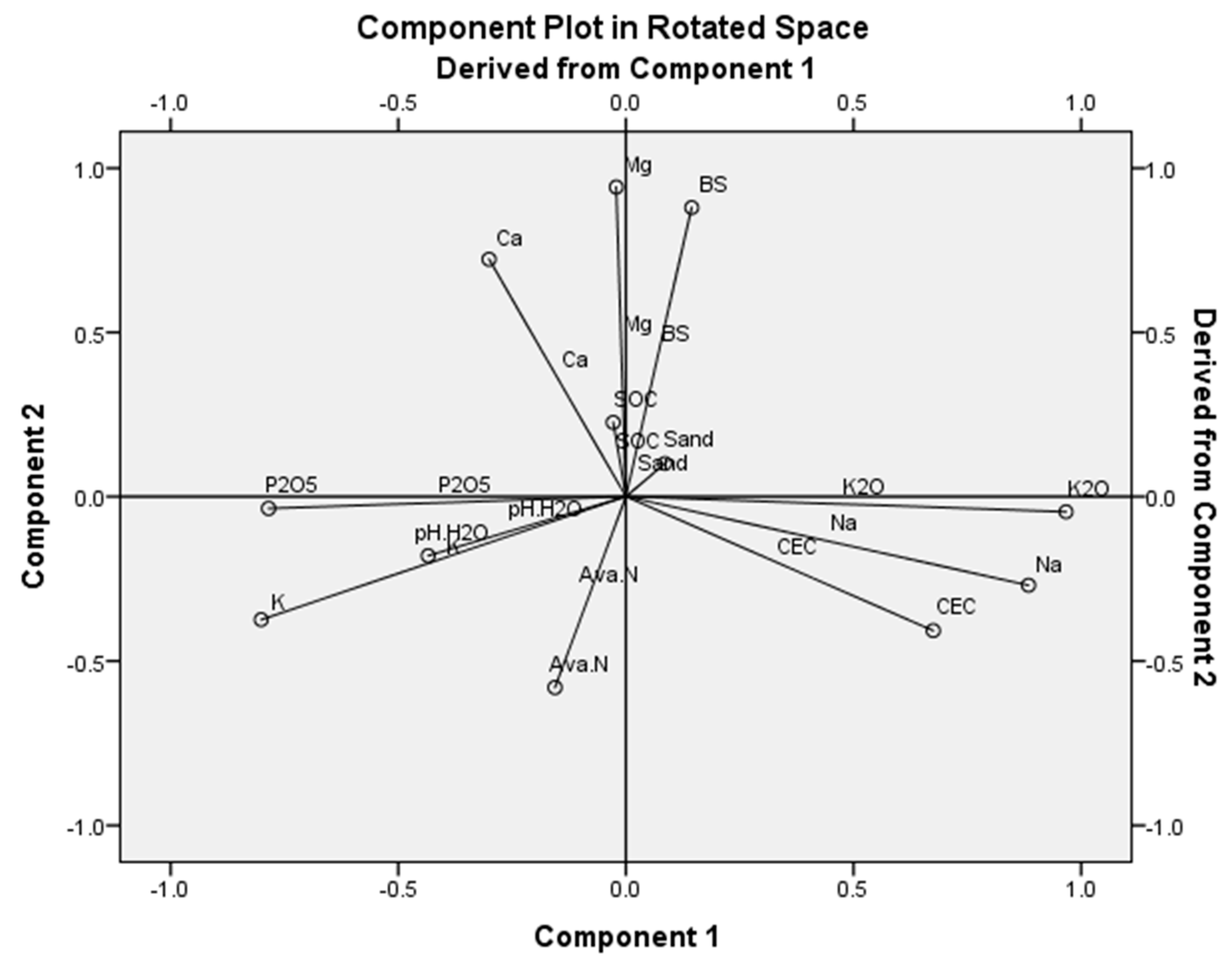
3.2.1. Correlation among Soil Properties

Variables of soil characteristics were distributed into three components through PCA (Table 4). Factors were extracted using PCA and Varimax rotation with Kaiser Normalization. Based on the eigenvalue’s threshold of >1, five components met the criteria. However, some components had either low loadings (<0.4) for all the variables or had significantly high loadings for the same variable across multiple components (multicollinearity). A three-component solution accounting for 70% variance was the best compromise. Similarly, the resulting Kaiser–Meyer–Olkin (KMO) value of 0.5 justifies the sampling adequacy of the sample. Bartlett’s test of sphericity was significant (<0.00001) suggesting correlation between the variables albeit with multicollinearity possibility [42].
F1 was associated with exchangeable K (negative), Na (positive), CEC (positive), plant available P (negative), plant available K (positive), and pH (negative). F2 was described by exchangeable cations (Mg and Ca) and base saturation. F3 dimension was defined by sand and available N (positive) and SOC (negative). Two-dimensional component loading plots, visualizing the relationships among the soil attributes, are presented in Figure 2.
As shown by the length of the vectors, plant available P, base saturation, exchangeable Mg and Na were highly influential in the variation of soil properties. Available P correlated negatively with plant available K. Mg, Ca, and BS were strongly positively correlated.
Small angles between the vectors represent a strong positive correlation. An angle of about 90 degrees indicates absence of correlation, while large angles of close to 180 degrees suggest a negative correlation. The length of the vectors is directly proportional to the influence of the variable (communality).
Consequently, five variables were selected for cluster analysis based on discriminating effect and correlation. From factor 1, plant available K (highly discriminating) and available P (negative correlation with K) were selected. BS (highly discriminating) was selected from factor 2, while sand (highly discriminating) and OC (negative correlation with SOC) were selected from factor 3.

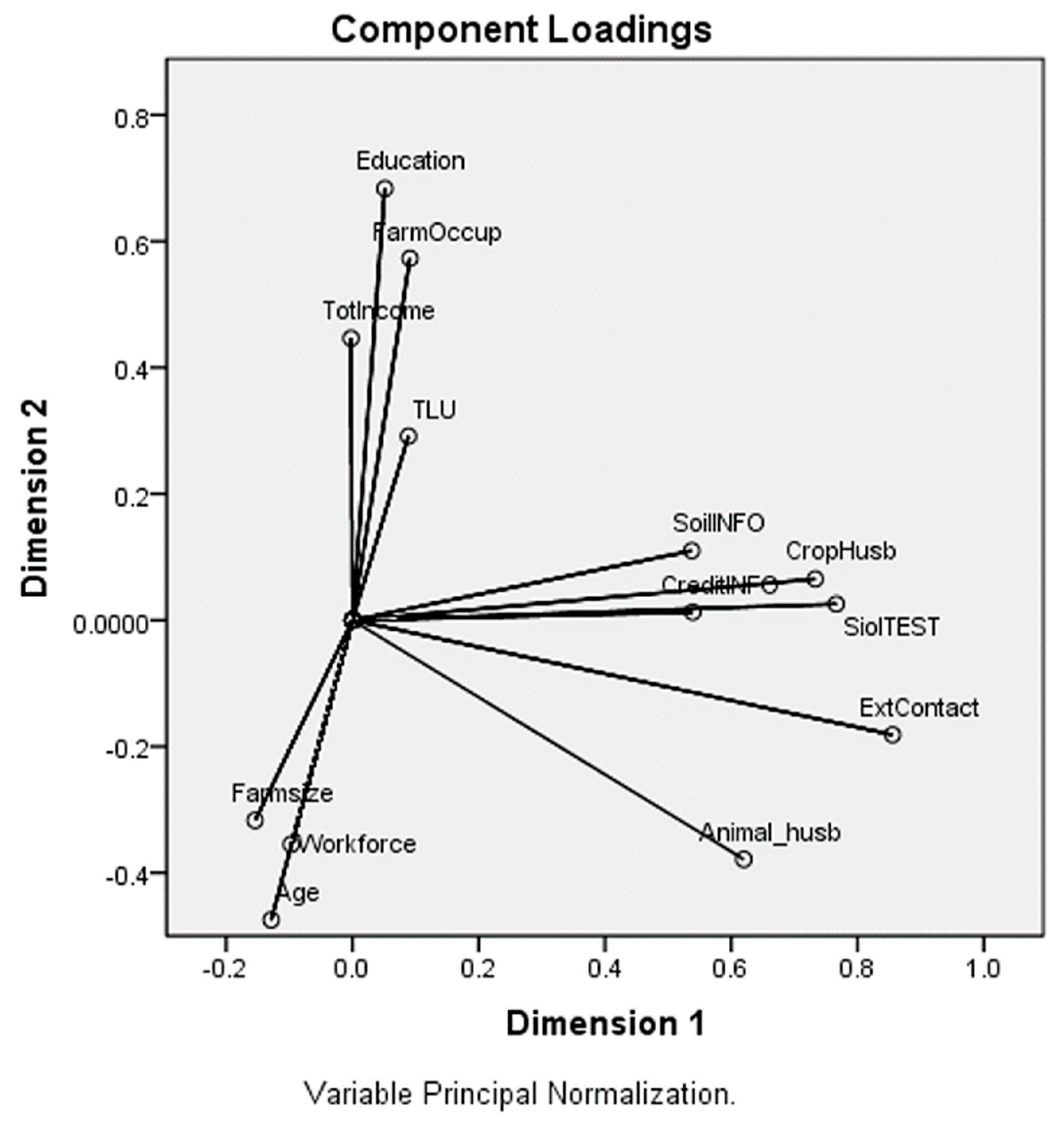
3.2.2. Principal Component Analysis of Socio-Economic Variables

All the 17 socio-economic variables (see Table 2) were submitted to the model with the number of dimensions retained at default (2). However, the two-dimensional solution accounted for only 39.3% of the variance (not plausible), implying that more information could be provided with additional dimensions. While six components were desirable (eigenvalues greater than one and accounting for more than 60% variance), the fourth and fifth components had low Cronbach’s alpha scores (low reliability). Dimension was then set at four and CATPCA performed again. This time, the fourth component had only one variable with a loading score of >0.4. The general rule is to retain components with at least four variables with a loading score >0.6 [43]. We therefore explored the data with a three-component solution while setting the threshold score loading at 0.4, which is considered a fair cut-off [44,45]. The results for the final analysis, which was run based on 13 variables and with 3 dimensions, are displayed (Table 5). Some variables that were initially included in the model were omitted from the repeat analyses due to high loading scores in more than one principal components [32]. These variables include gender, farming experience, family size, and access to agribusiness training.
Roughly 50% of the household variability was explained by the first 3 PCs. The first PC was associated with variables related to access to agricultural information. Education level of household head and total family income registered high positive loadings with PC2. Question on whether farming was the primary occupation for the household head, had high positive loading too, for this component. On the other hand, the age variable loaded negatively high. The third component was associated with farm size, number of livestock, and family workforce, all of which loaded positively high. Considering their independence, these dimensions constitute a good starting point for a consistent categorization of households. Two-dimensional component loading plots (Figure 3) were generated to provide a visualization of the relationships among the socio-economic factors.
There was a strong correlation among the information-related variables, namely contact with agricultural extension, access to information on soil, crops, livestock, and credit. Figure 3 suggests that a priori three classes of household characteristics can be identified in the study area following the associations between the determinant variables.

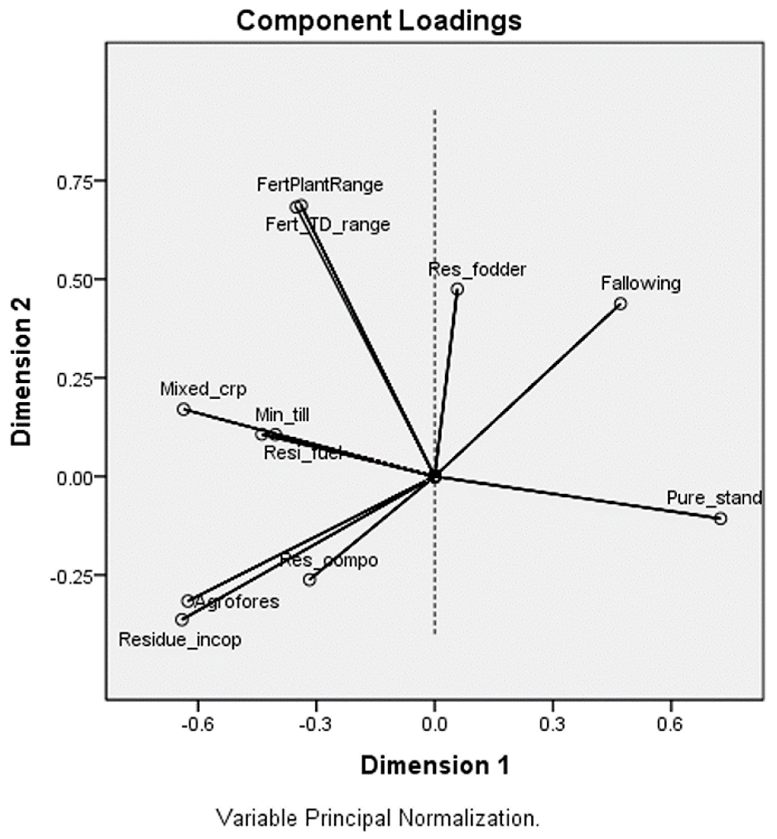
3.2.3. Principal Component Analysis of Soil Fertility Management Practices

Soil fertility management practices were distributed into three principal components through CATPCA using principal normalization. CATPCA was first performed with all the 15 soil fertility management-related variables, with 2 default dimensions. The resulting solution accounted for only 40% of the variance, which is considered too low, and thus a need for more dimensions. The analysis was repeated with dimensions number set at 10. The first four components had eigenvalue greater than one and accounted for 63% of the variance. However, the fourth PC had a low Cronbach’s alpha of 0.214 (low reliability). The results of the final analysis were performed with 11 variables. Attributes with loadings below 0.4 were omitted, including residue application, burning of crop residue, manure application, and intercropping. A3-dimension solution is displayed (Table 6).
About 53% of variability in soil fertility management was explained by the first three PCs. PC1 was correlated positively with pure stand cropping and fallowing, and negatively with mixed cropping, agroforestry, and minimum tillage. PC2 was associated with fertilizer usage rates both at planting and top dressing. The third component was related to residue compositing (positive) and residue use for fodder and fuel (both negative).
Visualization of the relationships among the soil fertility management practices is presented (Figure 4).
The relationships between soil fertility management practices, which are represented by their correlations with their PCs, are shown by vectors pointing toward the category with the highest score. The length of the vectors reflects the influence of the variables in relation to variation in soil fertility management practices. Fertilizer application rate and pure stand cropping were highly influential in PC1 and PC2, respectively. The small angle between fertilizer application rate during planting and growth reflects a strong positive correlation between the two variables. On the other hand, a large angle (approximately 180 degrees) between pure stand and mixed cropping shows a strong negative correlation. Figure 4 suggests that a priori four classes of field characteristics can be identified across the studied farming households.

3.3. Clustering and Characterization of Farm Types Based on Soil Characteristics

Soil variables with the highest loading as revealed by PCA were selected for inclusion in the cluster analysis. A non-hierarchical two-step clustering approach was used. Two clusters were automatically determined based on Bayesian Information Criterion (BIC). However, upon close examination of the retained clusters with respect to the field observations [37], the classification was not very meaningful. The solution was repeated with three clusters that seemed representative of the farm households in the study sites. Cluster membership was 14 (20.6%), 24 (35.3%) and 30 (44.1%) households for clusters 1, 2, and 3, respectively. The size ratio between the smallest and largest cluster was 2.14 (a fairly commendable ratio). The overall silhouette measure of cluster cohesion and separation value was 0.5, indicating a fair assignment of data points to cluster centers [38]. The final clusters obtained were profiled and assigned names: Farm type (FT) 1, 2, and 3.

3.3.1. Tendencies of Soil Properties across Farm Types

Differences in soil properties between clusters were examined based on cluster membership variable, using one-way ANOVA, and results presented in Table 7.
The distribution of clusters was strongly significant (p < 0.05) across all the selected soil parameters except for base saturation and sand particle composition, which were weakly significant (p < 0.1).
Cluster 1 farms have low exchangeable bases (K and Mg), available P, pH, and SOC. These farms have higher values for CEC, plant available K, and Na+ concentration. Cluster 2 farms are characterized by higher exch. Mg, available P, and SOC. Farms in cluster 3 have higher concentration of exch. K and pH values. Overall, fields within farm type 2 and 3 were more fertile than those in farm type 1, as indicated by the SQI. Farms in FT2 exhibited higher base saturation and exchangeable Ca concentration and SOC compared to FT3.

3.3.2. Socio-Economic Characteristics across the Farm Types

Households’ socio-economic variables were correlated with the identified farm types and results presented in Table 8 and Table 9. The distribution of farm types in relation to household socio-economic characteristics differed significantly across PC2 (personal attributes) and PC3 (farm size and other wealth indicators). Specifically, farm size, household income, family size, and livestock volume were important in delineating farm types. Cluster 3 has averagely larger farms compared to clusters 1 and 2. There is a slight farm type differentiation across household income (p < 0.1). Farms in cluster 1 had lower average income, while cluster 3 had highest income.
Proportionally, the majority of households within farm type 1 were male-headed, younger, educated beyond secondary school level, and with smaller family size. Farm type 3 farms were characterized by larger family size, higher workforce, and larger livestock units. Farm type 2 farms consisted of mainly older female household heads with medium family size, farm size, and income.
Farming was the primary occupation for household heads in farm type 1, who had a higher education level and income compared to their counterparts in farm type 2. Comparatively, farms in cluster 1 had higher access to soil testing services and financial (credit) information. Members of farm type 2 had a higher access to animal husbandry information, larger farm size, livestock, and more family members working on the farm.

3.3.3. Patterns of Soil Fertility Management Practices across Farm Types

Farm characterization based on soil fertility management characteristics differed significantly across the three principal components (Table 10): PC1 (mode of cropping), PC2 (intensity of fertilizer application), and PC3 (utilization of organic resources). Specifically, farm types were significantly different across fallowing practices (p < 0.05), the intensity of fertilizer application (p < 0.05), and utilization of crop residue for fuel (p < 0.1). Proportionally, more farmers in the farm type 2 category practiced fallowing. Farm type 3 farms exhibited higher fertilizer application rates for both planting and top dressing, while farm type 2 consists of farms with modest fertilizer consumption. A higher proportion of farmers in farm type 3 used crop residues as fuel.
Noticeably, cluster 1 farms are associated with mixed cropping, intercropping, and residue incorporation. Fertilizer application intensity is low, and farmers were very unlikely to compost crop residues. Farms in cluster 2 have proportionally high cases of fallowing and pure stand cropping, with modest fertilizer application rates, and composting of crop residues. Cluster 3 farms are characterized with high fertilizer application, high propensity to agroforestry and compositing of crop residues, and higher use of residue for fodder and fuel.

4. Discussion

The classification of farms segmented farm households into three clusters based on the influential soil properties determined by PCA. The conducted field quality classification yielded reasonable discrimination of soil fertility conditions across household farms. There was significant variation in soil fertility status between the three identified farm types as indicated by differences in the averages of key soil attributes, including pH, SOC, CEC, plant available plant K2O, available P, Base saturation, sand proportions, and exchangeable bases. The significant differences in SQI averages suggest a consistent variation in soil fertility across the three farm types, delineating the farms as low fertility (cluster 1), moderate fertility (2), and high fertility (3). It is, however, important to note that values of soil fertility indicators for most samples were above average levels based on published SQI thresholds [46]. This could be due to the generally fertile soils in the region, which is in fact considered a high agricultural potential area [47]. The variability in soil properties could be attributed to differential soil fertility management practices dictated by households’ socio-economic characteristics.
Farm type 1 farms were characterized by low values for available P, pH, SOC, and exchangeable bases (K and Mg). The values for P and SOC were very low, and the soils were moderately acidic [46]. Nevertheless, the average sand levels are generally within the acceptable range (<50%) [46]. Higher distribution of sand (course particles) could be ascribed to the loss of finer particles due to erosion [48].
Studies on African farming systems (e.g., [49,50]) have shown that the magnitude of SOC tended to vary between farm types. Increase in SOC and total N has been positively correlated with soil structure improvement [9]. The low fertility of farms in this cluster could be attributed to low use of organic and inorganic fertilizer and composted crop residues. The availability of high organic matter influences soil microbial functional diversity [51], but the use of inorganic fertilizer can have a negative impact on soil biota [52]. Socio-economically, households in cluster 1 had smaller family sizes and smaller farm sizes with low income. These variables constitute the key household characteristics that have been used to explore farming system diversity [53]. The low consumption of fertilizer in this farm type could be attributed to low on-farm income, limiting farmer’s access to soil fertility resources [32]. There is strong evidence worldwide supporting the link between poverty and land degradation [51]. Ref. [54] argues that “Poor soils make people poorer” and “poor people make soils worse.” Alternatively, this cluster consists of households with young families with the household head most likely to be in formal employment considering a high proportion have attained above high school education. This would imply that their participation in farming is largely on a part-time basis. Smaller land sizes are expected in this cluster, since land is inherited by the household head, thus fragmentation into smaller parcels [53].
Cluster 2 farms have moderate average values for plant available K, clay, pH, CEC, and exchangeable Ca. The fields have high SOC content, BS, and sand content. Moderate fertility status in these fields could be explained by the modest fertilizer application rates, less agroforestry, less residue incorporation (Table 8). The proportionally higher cases of fallowing contribute to the restoration of soil nutrients. Land use studies have shown that converting non-agricultural land into cultivated fields leads to decline in nutrients [55,56]. The households within this cluster are largely headed by older females with high farming experience and access to extension. Family sizes are moderate (larger than cluster 1) with above-average resource endowments in regard to farm size, income, and livestock units. These results are consistent with the findings of [53] in Ghana, which reported a positive correlation between family size, livestock size, and the age of the household head. In their typology of rural farm households, Refs. [32,57] found that age was a significant discriminant of cluster membership in Kenya. However, in other findings, none of the family’s head attributes nor socio-economic variables predicted cluster membership (cf. [31]). In our study, age was less discriminant, perhaps due to the diverse characteristics of the farming households in the study area.
Farms in cluster 3 were the most fertile as shown by high values for clay content, pH and exchangeable K, and moderate SOC. The difference in SOC between farm type 2 and 3 could be due to the effect of fallowing in the former, which allows for the build-up of organic matter from the accumulation of litter [56]. Fertilizer application, agroforestry. and composting of crop residues observed among the farms in this category are important contributors to soil fertility. Agroforestry practices have been shown to increase agricultural land’s capacity to sequester C and N [58]. The soil aggregate stability can also be enhanced by agroforestry through abundant fine roots (root exudates), thick litter layer, and rich soil binding agents [9]. Soil fertility management practices such as incorporation of crop residues increases soil carbon stocks [59]. It needs to be mentioned again that besides of its positive impacts on soil fertility, the use of inorganic fertilizers can also have a negative effect on soil biota as well as on the quality of surface and ground water, especially in the long term [52,60]. Similarly, the households in farm type 3 are characterized by high income, larger farms, high livestock volume, and larger families and workforce, which constitute key indicators of wealth [32,61]. This clustering is consistent with [32], which conducted a study in East Africa in which farms that belong to a wealthier farm type were characterized by larger livestock volume, large farms with cash crops, and high income mostly generated from farming activities. The influence of income (especially off-farm) in technology adoption is widely acknowledged [37]. Resource-endowed households have ready access to large volumes of inorganic fertilizers and manure [10]. In addition to contributing to household income, livestock provides manure, which is used to enhance soil fertility. Manure and other organic resources are critical in enhancing soil organic matter, nitrogen, phosphorus and other plant nutrients. Soil organic matter is critical for soil’s overall health, namely the soil’s capacity and sustainability to function as a living ecosystem. However, like many parts in SSA, the use of manure in Kenya is constrained by limited availability and poor quality [62,63]. In this study, the intensity of household’s consumption of animal manure is implicitly implied from the livestock volume (TLU). However, we note that the actual determination of the amount of manure used per unit area would have been more interesting. Farm labor, which is often dictated by the household size (positively correlated), is a key driver of technology adoption and a major indicator of household diversity [32,64]. Farming is the main occupation of the household heads, with the majority of them having attained lower than high school level education. A high degree of dedication to farming is thus expected and commitment to improve agricultural productivity (evident from higher fertilizer application rate) [32]. Operational management and labor allocation have been shown to influence farm productivity and the efficiency of resource utilization [3]. Households in this farm type have a high propensity of access to agricultural advice, including information on soil, crop, and livestock husbandry, which may also have contributed to sound soil fertility management [65].

5. Conclusions

The smallholder farming systems in most parts of SSA are highly heterogenous in terms of both biophysical and socio-economic characteristics. The extensive variability in soil fertility is a function of both short and long-term conditions associated with soil fertility management activities implemented over soils with inherently diverse properties. A host of socio-economic factors, including farm preferences, prices, and production objectives, further magnify farm household’s heterogeneity.
Farming systems in the upper Eastern Kenya were typified into three farm types, representing infertile farms (FT1), moderately fertile farms (FT2) and fertile farms (FT3).
FT1 are characterized by low values for important soil fertility indicators, including SOC, pH, CEC, available P, and exchangeable bases (K and Mg). On the account of soil fertility management practices, the low fertility could be explained by low application of fertilizer and organic resources. In turn, the observed management practices are influenced by smaller household size, lower income, and smaller farm size.
FT2 have higher levels of SOC, available P, exchangeable Mg, and moderate measurements for CEC, plant available K, and pH. The possible determinants of the observed fertility status include fallowing, the use of composted residues (manure), and above-average fertilizer application rates. The correlated household characteristics include moderate income, family size, and farm size. FT3 farms exhibit relatively desirable values for key soil fertility indicators, including SOC, pH, CEC, plant available plant available K, available P, and exchangeable bases (K and Mg). In relation to soil fertility management practices, the high fertility could be attributed to the high application rate of fertilizer and organic resources. Similarly, the observed management practices are influenced by favorable household socio-economic conditions, including larger household size, higher income, and larger farm size.
Characterization of farms based on the various parameters including resource endowment reveals imbalanced farm resource flows, suggesting a need to address the inequality in farm resource availability to reduce high soil quality variability and enhance the productivity and sustainability among smallholder farming systems. Results suggest that resource-inadequacy poses a threat to soil health and the environment at large. The knowledge of both biophysical and socio-economic variability is critical in appreciating the potential of individual farm households and to spearhead location-specific interventions to facilitate improved targeting of soil fertility-enhancing technologies, sustainable crop agricultural practices, and informed policy support. The findings of this study are a good starting point for efficient soil fertility management through a tailored innovative and integrated approach.

Author Contributions

Conceptualization, A.W., E.T.K. and Á.C.; methodology, A.W., E.T.K. and Á.C.; software, A.W.; validation, E.T.K., Á.C. and M.Z.; formal analysis, A.W., Á.C., B.R., J.P. and M.Z.; investigation, A.W., E.T.K. and Á.C.; resources, E.M. and Á.C; data curation, A.W. and Á.C.; writing—original draft preparation, A.W.; writing—review and editing, E.T.K., Á.C., T.S., B.R., J.P., M.Z. and E.M.; visualization, A.W., B.R., J.P. and M.Z.; supervision, E.T.K., Á.C., E.M. and T.S.; project administration, A.W., Á.C. and E.M.; funding acquisition, E.M. All authors have read and agreed to the published version of the manuscript.

Funding

This work was supported by the Tempus Foundation through Hungarian University of Agriculture and Life Sciences in Gödöllő, Hungary on the Stipendium Hungaricum Scholarship (Grant Number 99674). The research was supported by the project “Preparation for the transition to circular economy in the case of agricultural and green waste” of Environment and Energy Efficiency Operational Programme grant scheme of Ministry of Technology and Industry Hungary under grant no.: KEHOP-3.2.1-15-2021-00037. This research was supported by the Agrotechnology National Laboratory Development project (ID: 2022-2.1.1-NL-2022-00006) which was implemented with the support of the Ministry of Culture and Innovation from the National Research, Development and Innovation Fund (2022-2.1.1-NL) based on a Grant Agreement (NKFIH-3524-1/2022) with the National Research, Development and Innovation Office.

Data Availability Statement

The data related to this study are available for scientific purposes upon request from the corresponding author.

Acknowledgments

We acknowledge the logistical support received from the Kenya Agricultural and Livestock Research Organization (KALRO). Special thanks to Evans Mutuma (KALRO) and József A. Tóth (MATE) for their tremendous support during soil sampling and data collection. We thank Doreen Kanario for assisting with the questionnaire administration. Authors are also grateful to all the farmers and agricultural extension officers who assisted and participated in the survey.

Conflicts of Interest

The authors declare no conflict of interest.

References

  1. Tittonell, P.; Vanlauwe, B.; Leffelaar, P.A.; Shepherd, K.D.; Giller, K.E. Exploring diversity in soil fertility management of smallholder farms in western Kenya: II. Within-farm variability in resource allocation, nutrient flows and soil fertility status. Agric. Ecosyst. Environ. 2005, 110, 166–184. [Google Scholar] [CrossRef]
  2. Zingore, S.; Murwira, H.K.; Delve, R.J.; Giller, K.E. Influence of nutrient management strategies on variability of soil fertility, crop yields and nutrient balances on smallholder farms in Zimbabwe. Agric. Ecosyst. Environ. 2007, 119, 112–126. [Google Scholar] [CrossRef]
  3. Tittonell, P.; Leffelaar, P.A.; Vanlauwe, B.; van Wijk, M.T.; Giller, K.E. Exploring diversity of crop and soil management within smallholder African farms: A dynamic model for simulation of N balances and use efficiencies at field scale. Agric. Syst. 2006, 91, 71–101. [Google Scholar] [CrossRef]
  4. Turmel, M.S.; Speratti, A.; Baudron, F.; Verhulst, N.; Govaerts, B. Crop residue management and soil health: A systems analysis. Agric. Syst. 2015, 134, 6–16. [Google Scholar] [CrossRef]
  5. Ojiem, J.O.; de Ridder, N.; Vanlauwe, B.; Giller, K.E. Socio-ecological niche: A conceptual framework for integration of legumes in smallholder farming systems. Int. J. Agric. Sustain. 2006, 4, 79–93. [Google Scholar] [CrossRef]
  6. Gómez-Limón, J.; Berbel, J.; Arriaza, M. MCDM Farm System Analysis For Public Management Of Irrigated Agriculture. In Handbook On Operations Research In Natural Resources In International Series In Operations Research And Management Science; Weintraub, A., Bjorndal, T., Epstein, R., Romero, Y., Eds.; Páginas, Kluwer: New York, NY, USA, 2007; pp. 93–114. [Google Scholar]
  7. Sheahan, M.; Olwande, J.; Kirimi, L.; Jayne, T.S. Targeting of Subsidized Fertilizer Under Kenya’s National Accelerated Agricultural Input Access Program (NAAIAP): Food Security Collaborative Working Papers 188572; Michigan State University, Department of Agricultural, Food and Resource Economics: East Lansing, MI, USA, 2014. [Google Scholar]
  8. Bouma, J.; Reyes-Garcia, V.; Huanca, T.; Arrazola, S. Understanding conditions for co-management: A framed field experiment amongst the Tsimane’, Bolivia. Ecol. Econ. 2017, 141, 32–42. [Google Scholar] [CrossRef]
  9. Zou, X.; Zhu, X.; Zhu, P.; Singh, A.K.; Zakari, S.; Yang, B.; Chen, C.; Liu, W. Soil quality assessment of different Hevea brasiliensis plantations in tropical China. J. Environ. Manag. 2021, 285, 112147. [Google Scholar] [CrossRef]
  10. Chikowo, R.; Zingore, S.; Snapp, S.; Johnson, A. Farm typologies, soil fertility variability and nutrient management in smallholder farming in Sub-Saharan Africa Farm typologies, soil fertility variability and nutrient management in smallholder farming in Sub-Saharan Africa. Nutr. Cycl. Agroecosystems 2014, 100, 1–18. [Google Scholar] [CrossRef]
  11. Braun, A.R.; Smaling, E.M.A.; Muchugu, E.I.; Shepherd, K.D.; Corbett, J.D. Maintenance and improvement of soil productivity in the highlands of Ethiopia, Kenya, Madagascar and Uganda An inventory of spatial and non-spatial survey. Africa Highlands Initiative Techical Report Series; International Centre for Research in Agroforestry: Nairobi, Kenya, 1997; 129p. [Google Scholar]
  12. Shepherd, K.; Ohisson, E.; Okalebo, J.; Ndufa, J. Potential impact of agroforestry on soil nutrient balances at the farm scale in the East African highlands. Fertil. Res. 1996, 44, 87–99. [Google Scholar] [CrossRef]
  13. Barrett, C.B.; Marenya, P.P.; Mcpeak, J.; Minten, B.; Murithi, F.; Oluoch-Kosura, W.; Place, F.; Randrianarisoa, J.C.; Rasambainarivo, J.; Wangila, J. Welfare dynamics in rural Kenya and Madagascar. J. Dev. Stud. 2006, 42, 248–277. [Google Scholar] [CrossRef]
  14. KNBS. 2019 Kenya population and Housing Census. Volume 1: Population by County and Sub-County; KNBS: Nairobi, Kenya, 2019. [Google Scholar]
  15. Jaetzold, R.; Schmidt, H.; Hornetz, B.; Shisanya, C. Natural conditions and farm management information, part C East Kenya. In Farm Management Handbook of Kenya, 2nd ed.; Ministry of Agriculture: Nairobi, Kenya, 2007; Volume II. [Google Scholar]
  16. IUSS Working Group WRB. World Reference Base for Soil Resources 2014, Update 2015. In International Soil Classification System for Naming Soils and Creating Legends for Soil Maps; World Soil Resources Reports No. 106; FAO: Rome, Italy, 2015. [Google Scholar]
  17. Roudier, P.; Hewitt, A.E.; Beaudette, D.E. A conditioned Latin hypercube sampling algorithm incorporating operational constraints. Digit. Soil Assessments Beyond-Proc. Fifth Glob. Work. Digit. Soil Mapp. 2012, 227–231. [Google Scholar] [CrossRef]
  18. Mulder, V.L.; de Bruin, S.; Schaepman, M.E. Representing major soil variability at regional scale by constrained Latin Hypercube Sampling of remote sensing data. Int. J. Appl. Earth Obs. Geoinf. 2012, 21, 301–310. [Google Scholar] [CrossRef]
  19. USDA. Sampling Soils for Nutrient Management; USDA: Washington, DC, USA, 2018. [Google Scholar]
  20. van Reeuwijk, L. Procedures for Soil Analysis, 6th ed.; International Soil Reference and Information Centre (ISRIC): Wageningen, The Netherlands, 2022. [Google Scholar]
  21. Gillman, G.P.; Sumpter, E.A. Modification to the compulsive echange method for measuring exchange characteristics of soils. Aust. J. Soil Res. 1986, 24, 61–66. [Google Scholar] [CrossRef]
  22. Ross, D.S.; Ketterings, Q. Recommended Methods for Determining Soil Cation Exchange Capacity. In Recommended Soil Testing Procedures for the Northeastern United States, 3rd ed.; Wolf, A., McGrath, J., Eds.; Agricultural Experiment Stations of Connecticut: New Haven, CT, USA, 2011. [Google Scholar]
  23. Mehlich, A. Mehlich-3 soil test extractant: A modification of Mehlich-2 extractant. Commun. Soil Sci. Plant Anal. 1984, 15, 1409–1416. [Google Scholar] [CrossRef]
  24. Carte, M.R.; Gregorich, E.G. Soil Sampling and Methods of Analysis, 2nd ed.; Carter, M.R., Gregorich, M.R., Eds.; CRC Press: Boca Raton, FL, USA, 2008. [Google Scholar]
  25. Bremmer, J.M.; Mulvaney, C.S. Nitrogen-Total. Methods of soil anaylsis. Part 2. In Chemical and Biological Properties; Page, A.L., Miller, R.H., Keeney, D.R., Eds.; American Society of Agronomy, Soil Science Society of America: Madison, WI, USA, 1982; pp. 526–595. [Google Scholar]
  26. Egnér, H.; Riehm, H.; Domingo, W.R. Untersuchungen über die chemische Bodenanalyse als Grundlage für die Beurteilung des Nahrstoffzustandes der Böden. II. Chemische Extraktionsmethoden zur Phosphor- und Kaliumbestimmung. K. Lantbr. Ann. 1960, 26, 199–215. [Google Scholar]
  27. Haluschak, P.; Laboratory Methods of Soil Analysis. Canada–Manitoba Soil Survey. 2006; 133p. Available online: https://www.gov.mb.ca/agriculture/soil/soil-survey/pubs/laboratory_methods_of_soil_analysis.pdf (accessed on 5 April 2023).
  28. Giller, K.E.; Tittonell, P.; Rufino, M.C.; van Wijk, M.T.; Zingore, S.; Mapfumo, P.; Adjei-Nsiah, S.; Herrero, M.; Chikowo, R.; Corbeels, M.; et al. Communicating complexity: Integrated assessment of trade-offs concerning soil fertility management within African farming systems to support innovation and development. Agric. Syst. 2011, 104, 191–203. [Google Scholar] [CrossRef]
  29. Pacini, G.C.; Colucci, D.; Baudron, F.; Righi, E.; Corbeels, M.; Tittonell, P.; Stefanini, F.M. Combining multi-dimensional scaling and cluster analysis to describe the diversity of rural households. Exp. Agric. 2013, 50, 376–397. [Google Scholar] [CrossRef] [Green Version]
  30. Alary, V.; Messad, S.; Taché, C.; Tillard, E. Approach to the diversity of dairy farm systems in Reunion. Rev. Elev. Méd. Vét. Pays Trop. 2002, 55, 285–297. [Google Scholar] [CrossRef] [Green Version]
  31. Dossa, L.H.; Abdulkadir, A.; Amadou, H.; Sangare, S.; Schlecht, E. Exploring the diversity of urban and peri-urban agricultural systems in Sudano-Sahelian West Africa: An attempt towards a regional typology. Landsc. Urban Plan. 2011, 102, 197–206. [Google Scholar] [CrossRef]
  32. Tittonell, P.; Muriuki, A.; Shepherd, K.D.; Mugendi, D.; Kaizzi, K.C.; Okeyo, J.; Verchot, L.; Coe, R.; Vanlauwe, B. The diversity of rural livelihoods and their influence on soil fertility in agricultural systems of East Africa—A typology of smallholder farms. Agric. Syst. 2010, 103, 83–97. [Google Scholar] [CrossRef]
  33. Hair, J.F.; Black, W.C.; Babin, B.; Anderson, R. Pharmaceutical Quality by Design: A Practical Approach. In Multivariate Data Analysis, 7th ed.; Pearson Education Limited: Essex, UK, 2010. [Google Scholar] [CrossRef]
  34. Samuels, P. Advice on Exploratory Factor Analysis; Birminghan City University Technical Report; Birminghan City University: Birmingham, UK, 2017. [Google Scholar]
  35. Linting, M.; Meulman, J.J.; Groenen, P.J.F.; van der Kooij, A.J. Non-linear principal components analysis: Introduction and application. Psychol. Methods 2007, 12, 336–358. [Google Scholar] [CrossRef] [PubMed] [Green Version]
  36. Meulman, J.J.; Heiser, W. IBM SPSS Categories 19; SPSS Inc.: Armonk, NY, USA, 2010. [Google Scholar]
  37. Goswami, R.; Chatterjee, S.; Prasad, B. Farm types and their economic characterization in complex agro-ecosystems for informed extension intervention: Study from coastal West Bengal, India. Agric. Food Econ. 2014, 2, 5. [Google Scholar] [CrossRef] [Green Version]
  38. Jain, R.; Koronios, R. Innovation in the cluster validating techniques. Fuzzy Optim. Decis. Mak. 2008, 7, 233–241. [Google Scholar] [CrossRef]
  39. Kuria, A.W.; Barrios, E.; Pagella, T.; Muthuri, C.W.; Mukuralinda, A.; Sinclair, F.L. Farmers’ knowledge of soil quality indicators along a land degradation gradient in Rwanda. Geoderma Reg. 2018, 16, 14. [Google Scholar] [CrossRef]
  40. Wawire, A.W. Analysis of Soil Quality, Farmers’ Knowledge and Management Practices in Mount Kenya East Region. Ph.D. Dissertation, Doctoral School of Environmental Sciences, Hungarian University of Agriculture and Life Sciences, Gödöllő, Hungary, 2021; 208p. [Google Scholar]
  41. Storck, H.; Emana, B.; Adnew, B.; Borowiccki, A.; Woldehawariat, S. Farming Systems and Resource economics in the Tropics: Farming System and Farm Management Practices of Smallholders in the Hararghe Highland; Wissenschaftsverlag Vauk: Kiel, Germany, 1991; Volume II. [Google Scholar]
  42. Finch, W.H. Exploratory Factor Analysis. In Handbook of Quantitative Methods for Educational Research; Teo, T., Ed.; Sense Publishers: Rotterdam, The Netherlands, 2013; pp. 1–15. [Google Scholar]
  43. Stevens, J. Applied Multivariate Statistics for the Social Sciences; Routledge: New York, NY, USA, 1992. [Google Scholar]
  44. Comrey, L.A.; Lee, H.B. A First Course in Factor Analysis, 2nd ed.; Lawrence Eribaum Associate: Hillside, NJ, USA, 1992. [Google Scholar]
  45. Field, A. Discovering Statistics Using SPSS; Sage Publications, Inc.: London, UK, 2005. [Google Scholar]
  46. Amacher, M.C.; O’Neill, K.P.; Perry, C.H. Soil Vital Signs: A New Soil Quality Index (SQI) for Assessing Forest Soil Health; U.S. Department of Agriculture, Forest Service, Rocky Mountain Research Station: Fort Collins, CO, USA, 2007. [Google Scholar] [CrossRef]
  47. Ariga, J.; Jayne, T.S. Fertilizer in Kenya: Factors Driving the Increase in Usage by Smallholder Farmers, 1990–2007. Yes Afr. Can Success Stories A Dyn. Cont. 2011, 269–288. [Google Scholar]
  48. Tuo, D.; Xu, M.; Gao, G. Relative contributions of wind and water erosion to total soil loss and its effect on soil properties in sloping croplands of the Chinese Loess Plateau. Sci. Total Environ. 2018, 633, 1032–1040. [Google Scholar] [CrossRef]
  49. Dembe’le’, I.; Kone’, D.; Soumare’, A.; Coulibaly, D.; Kone’, Y.; Ly, B.; Kater, L. Fallows and field systems in Mali. In Nutrients on the Move: Soil Fertility Dynamics in African Farming Systems; Hilhorst, T., Muchena, F., Eds.; IIED: London, UK, 2000; pp. 83–102. [Google Scholar]
  50. Rotich, D.K.; Ogaro, V.N.; Wabuile, E.; Mulamula, H.H.A.; Wanjala, C.M.M.; Defoer, T. Participatory characterisation and on-farm testing in Mutsulio village, Kakamega District. In Pilot Project on Soil Fertility Replenishment and Recapitalisation in Western Kenya; Report No. 11; Kenya Agricultural Research Institute: Kakamega, Kenya, 1999. [Google Scholar]
  51. Tully, K.; Sullivan, C.; Weil, R.; Sanchez, P. The State of soil degradation in sub-Saharan Africa: Baselines, trajectories, and solutions. Sustainability 2015, 7, 6523–6552. [Google Scholar] [CrossRef] [Green Version]
  52. Kibblewhite, M.G.; Ritz, K.; Swift, M.J. Soil health in agricultural systems. Philos. Trans. R. Soc. B Biol. Sci. 2008, 363, 685–701. [Google Scholar] [CrossRef] [Green Version]
  53. Kuivanen, K.S.; Alvarez, S.; Michalscheck, M.; Adjei-Nsiah, S.; Descheemaeker, K.; Mellon-Bedi, S.; Groot, J.C.J. Characterising the diversity of smallholder farming systems and their constraints and opportunities for innovation: A case study from the Northern Region, Ghana. NJAS Wageningen J. Life Sci. 2016, 78, 153–166. [Google Scholar] [CrossRef]
  54. Hartemink, A.E. Poor soils make poor people and poor people make the soil worse. Manag. Trop. Sandy Soils Sustain. Agric. 2005, 107, 16–20. [Google Scholar] [CrossRef]
  55. Trumbore, S.; Brando, P.; Hartmann, H. Forest health and global change. Science 2015, 349, 819–822. [Google Scholar] [CrossRef] [PubMed] [Green Version]
  56. Willy, D.K.; Muyanga, M.; Mbuvi, J.; Jayne, T. The effect of land use change on soil fertility parameters in densely populated areas of Kenya. Geoderma 2019, 343, 254–262. [Google Scholar] [CrossRef]
  57. Bidogeza, J.C.; Berentsen, P.B.M.; De Graaff, J.; Oude Lansink, A.G.J.M. A typology of farm households for the Umutara Province in Rwanda. Food Secur. 2009, 1, 321–335. [Google Scholar] [CrossRef]
  58. Cong, W.F.; Hoffland, E.; Li, L.; Six, J.; Sun, J.H.; Bao, X.G.; Zhang, F.S.; Van Der Werf, W. Intercropping enhances soil carbon and nitrogen. Glob. Chang. Biol. 2015, 21, 1715–1726. [Google Scholar] [CrossRef]
  59. Segnini, A.; Posadas, A.; da Silva, W.T.L.; Milori, D.M.B.P.; Gavilan, C.; Claessens, L.; Quiroz, R. Quantifying soil carbon stocks and humification through spectroscopic methods: A scoping assessment in EMBU-Kenya. J. Environ. Manag. 2019, 234, 476–483. [Google Scholar] [CrossRef] [PubMed]
  60. Khan, M.N.; Mobin, M.; Abbas, Z.K.; Alamri, S.A. Fertilizers and their contaminants in soils, surface and groundwater, Encyclopedia of the Anthropocene. Encycl. Anthr. 2017, 5, 225–240. [Google Scholar] [CrossRef]
  61. Köbrich, C.; Rehman, T.; Khan, M. Typification of farming systems for constructing representative farm models: Two illustrations of the application of multi-variate analyses in Chile and Pakistan. Agric. Syst. 2003, 76, 141–157. [Google Scholar] [CrossRef]
  62. Ndambi, O.A.; Pelster, D.E.; Owino, J.O. Manure Management Practices and Policies in Sub-Saharan Africa: Implications on Manure Quality as a Fertilizer. Front. Sustain. Food Syst. 2019, 3, 29. [Google Scholar] [CrossRef] [Green Version]
  63. Waithaka, M.M.; Thornton, P.K.; Shepherd, K.D.; Ndiwa, N.N. Factors affecting the use of fertilizers and manure by smallholders: The case of Vihiga, western Kenya. Nutr. Cycl. Agroecosystems 2007, 78, 211–224. [Google Scholar] [CrossRef]
  64. Mugwe, J.; Mugendi, D.; Mucheru-Muna, M.; Merckx, R.; Chianu, J.; Vanlauwe, B. Determinants of the decision to adopt integrated soil fertility management practices by smallholder farmers in the central highlands of Kenya. Exp. Agric. 2009, 45, 61–75. [Google Scholar] [CrossRef] [Green Version]
  65. Gondwe, T.M.; Alamu, E.O.; Musonda, M.; Geresomo, N.; Maziya-Dixon, B. The relationship between training farmers in agronomic practices and diet diversification: A case study from an intervention under the Scaling Up Nutrition programme in Zambia. Agric. Food Secur. 2017, 6, 72. [Google Scholar] [CrossRef] [Green Version]
Figure 1. Map of Kenya showing the location of the study area (a), distribution of sampling sites within the study area (b), the spatial distribution of sampling points (c).
Agronomy 13 01101 g001
Figure 2. Plots of component loadings obtained from factor analysis describing the relationships among soil properties.
Agronomy 13 01101 g002
Figure 3. Correlation biplot showing the relationship between socio-economic variables.
Agronomy 13 01101 g003
Figure 4. Correlation biplot showing the relationship between soil fertility management practices.
Agronomy 13 01101 g004
Table 1. The selected soil properties variables for Factor analysis and clustering.
VariablesDefinitionMeasurement/Unit
CaExchangeable Calciumcmol/kg
MgExchangeable Magnesiumcmol/kg
NaExchangeable Sodiumcmol/kg
KExchangeable Potassiumcmol/kg
pHpH water
SOCTotal organic carbon%
CECSoil CEC%
P2O5Plant available Pmg/kg
NPlant available Nmg/kg
ClayClay content%
SandSand content%
SiltSilt content%
BSBase saturation%
K2OPlant available Kmg/kg
Table 2. The selected socio-economic characteristics and soil fertility management practices used for farm characterization.
VariablesDefinitionMeasurement/Unit
Household Socio-Economic Characteristics
GenderGender of the household head0 = female, 1 = male
AgeAge of household headYears
EducationHousehold head education level1 = below high school, 2 = above high school
Farming occupationFarming as primary occupation0 = no, 1 = yes
ExperienceYears in farming1 = below 20, 2 = above 20
Extension contactContact with extension in the last 5 years0 = no, 1 = yes
Soil infoAccess to training on soil management0 = no, 1 = yes
Soil testingsoil analysis has even been undertaken on farm0 = no, 1 = yes
Credit infoFarmer has ever received training on credit0 = no, 1 = yes
Crop informationFarmer has ever received training on crop
husbandry
0 = no, 1 = yes
Agribusiness infoFarmer has ever received training on agribusiness0 = no, 1 = yes
LivestockLivestock ownership0 = no, 1 = yes
Family sizeNumber of people in the familyCount
Farm sizeTotal size of landholding cultivated by
household
Acres
Household incomeAnnual household income (on-farm and
off-farm)
Ksh
Work forceNumber of household members actively
involved in farming
Count
TLUAggregated livestock assetsstandardized value
Cropping practices and soil fertility management
PCropPure crop stands practiced0 = no, 1 = yes
MixedMixed cropping practiced0 = no, 1 = yes
AgrofAgroforestry practiced0 = no, 1 = yes
IntCropIntercropping practiced0 = no, 1 = yes
ResidueFarm residues applied0 = no, 1 = yes
ManureManure applied0 = no, 1 = yes
MintillMinimum tillage practiced0 = no, 1 = yes
FallowFallowing practiced0 = no, 1 = yes
Residue incorpIncorporation practiced0 = no, 1 = yes
BurnBurning residues practiced0 = no, 1 = yes
CompostCompost manure applied0 = no, 1 = yes
FodderFarm organic materials used as fodder0 = no, 1 = yes
FuelFarm organic materials used as fuel0 = no, 1 = yes
Fert. Plant rateAmount of fertilizer used during plantingkg/ha
Fert.Topdress rateAmount of fertilizer used during for top
dressing
kg/ha
Table 3. Farm household demographic and socio-economic characteristics in upper Eastern Kenya.
ParameterCategoryNumber of Farmers
n = 69%Mean
GenderMale4159.4N/A
Female2840.6
EducationBelow High school3855.1N/A
High school and above3144.9
Farming typeCrop57.2N/A
Crop and livestock6492.8
Farming as primary occupationYes6492.8N/A
No57.2
Farming experience (years)<101826.1N/A
11–201318.8
21–302434.8
>301420.3
Extension ContactNo4362.3N/A
Yes2637.7
Soil infoNo6289.9N/A
Yes710.1
Soil testingNo5782.6N/A
Yes1217.4
Credit infoNo6492.8N/A
Yes57.2
Crop husbandry adviceNo5782.6N/A
Yes1217.4
Animal husbandry adviceNo6087N/A
Yes913
AgribusinessNo6898.6N/A
Yes11.4
AgeN/AN/AN/A46.7
Family sizeN/AN/AN/A5.2
Members active in farmingN/AN/AN/A3.0
Farm size (Ha)N/AN/AN/A3.5
Total income (Ksh *)N/AN/AN/A112,512.2
** TLU (Tropical livestock unit)N/AN/AN/A1.8
* 1 Kenya shilling (KES) = 0.0101 USD based on the average exchange rate at the time of data collection (March 2019). ** TLU is an aggregation of the different types of livestock. Conversion factors used are as follows: ox = 1.10, cow =1.0, heifer = 0.50, bull = 0.6, calves = 0.2, sheep and goats = 0.10, pigs = 0.20, and poultry = 0.01 [41].
Table 4. Principal component loadings of soil variables derived by principal components analysis using variable principal normalization.
VariableFactorCommunalities
123
K−0.812 0.786
Na0.877 0.855
CEC0.673 0.697
P2O5−0.770 0.821
K2O0.965 0.937
pH−0.443 0.239
Mg 0.921 0.890
Ca 0.736 0.623
BS 0.927 0.899
Sand 0.8570.848
SOC −0.4550.222
N 0.6430.624
Eigenvalues3.7992.9621.681
% of Variance31.65724.68514.006
Cumulative%31.65756.34270.348
Table 5. Principal component loadings of household socio-economic variables based on CATPCA analysis using variable principal normalization.
VariableDimensionTotal
123
Extension contact0.856 0.548
Soil info0.537 0.662
Soil testing0.767 0.454
Credit INFO0.539 0.208
Crop husbandry advice0.733 0.628
Animal husbandry advice0.620 0.255
Education 0.690 0.389
Tot income 0.444 0.773
age −0.477 0.302
Farm occupation 0.579 0.598
Farm size 0.7410.309
TLU 0.5930.577
Workforce 0.7100.529
Cronbach’s alpha0.7080.4550.4130.909 a
Total (eigenvalue)2.8891.7241.6176.231
% of variance22. 74714.08913.89150.727
a Total Cronbach’s alpha is based on the total eigenvalue.
Table 6. Principal component loadings of soil fertility management practices based on CATPCA analysis using variable principal normalization.
VariableDimensionTotal
123
Pure stand cropping0.724 0.538
Mixed cropping−0.635 0.435
Agroforestry−0.633 0.529
Minimum tillage−0.435 0.373
Fallowing0.478 0.408
Residue incorporation−0.646 0.538
Quantity of fertilizer (planting) 0.740 0.713
Fertilizer quantity (top dress) 0.732 0.717
Residue composted 0.6230.528
Residue used as fodder −0.6960.657
Residue used as fuel −0.4640.387
% of variance23.95115.76513.21952.936
Cronbach’s alpha0.6820.4660.3440.911 a
a Total Cronbach’s alpha is based on the total eigenvalue.
Table 7. Characterization of identified farm types based on p-value of one-way analysis of variance (equality of mean) of soil properties.
Cluster (Farm Types)TotalFSig.
Variable1 (n = 14)2 (n = 24)3 (n = 30)
Exch. K0.388b1.000a1.000a0.874168.1830.000
Exch. Mg0.512b0.958a0.733ab0.7674.9950.010
Exch. Na0.059a0.000b0.000b0.01326.1880.000
CEC16.448a8.167b8.033b9.81365.4070.000
BS%18.73019.08315.63317.4882.0740.132
Sand27.85727.95823.33325.8972.1590.124
AL-P2O55.286c828.717a740.510b620.272348.8510.000
AL-K2O195.357a13.125b9.233b48.92642.1990.000
pH.H2O4.879b5.083b6.103a5.49138.7430.000
SOC0.543bc1.398a0.835b0.97422.7970.000
SQI4.286b5.291a5.233a5.0593.4680.037
Each letter denotes a subset of cluster number means whose column proportions do not differ significantly (p < 0.05). SQI = soil quality index, calculated by summing up assigned threshold values for key selected soil variables for each field (see [46]).
Table 8. Characterization of identified farm types based on p-value of one-way analysis of variance (equality of mean) of socio-economic characteristics.
VariableClusterNMeanStd. DevMinMaxFSig.
Family size1144.7141.326370.9580.389
2245.1251.67618
3305.4331.695211
Total685.1761.620111
Farm size1142.4822.2020.256.003.6920.030
2242.8132.3290.2510.00
3304.5983.5120.5010.00
Total683.5323.0110.2510.00
TLU1141.5651.0830.62004.85001.4970.232
2241.4551.2590.00005.2000
3302.1331.8450.00007.0700
Total681.7771.5320.00007.0700
Workforce1143.0711.385150.8620.427
2242.6671.49416
3303.1671.39216
Total682.9711.42416
Age11441.07117.02220731.6170.206
22449.12512.0812675
33047.86713.6273074
Total6846.91214.0002075
Table 9. Comparison of households’ socio-economic characteristics across the identified farm types in upper Eastern Kenya.
VariableCategoryFarm Type (Cluster)Total%CoeffSig
1 (n = 14)2 (n = 24)3 (n = 30)
Freq%Freq%Freq%
GenderFemale535.71145.81240.028410.0770.855
Male964.31354.21860.04059
Income (Ksh)<75753.81052.61142.32848.3 0.130
75–15017.7421.1623.11119.0
150–225538.5421.1311.51220.7
>2250015.3623.1712.1
EducationPrimary and below535.71458.31963.338560.2070.218
High school and above964.31041.71136.73044
Farm occupationNo17.128.326.7570.0290.973
Yes1392.92291.72893.36393
Farming experience<20750.0833.31653.331460.1800.318
>20750.01666.71446.73754
Ext contactNo1071.41354.21963.342620.130.557
Yes428.61145.81136.72638
Soil infoNo1392.92291.72686.761900.0900.759
Yes17.128.3413.3710
Siol TESTNo1285.7833.32686.746680.1410.500
Yes214.3625.0413.31218
Credit INFONo14100.02187.52893.363930.1720.356
Yes00.0312.526.757
Crop husbandry adviceNo1285.72083.32480.056820.0590.887
Yes214.3416.7620.01218
Animal husbandry adviceNo14100.02187.52480.059870.2160.188
Yes00.0312.5620.0913
AgribizNo14100.024100.02996.767990.1360.526
Yes00.000.013.311
Table 10. Frequency distribution of soil fertility management characteristics across clusters (farm types) in Upper Eastern Kenya.
VariableCluster (Farm Types)Totalp-Value
1 (n = 14)2 (n = 24)3 (n= 30)
freq%freq%freq%
Pure standNo9a64.314a58.321a70.0440.606
Yes5a35.710a41.79a30.024
Mixed croppingNo3a21.411a45.810a33.3240.308
Yes11a78.613a54.220a66.744
AgroforestryNo10a71.418a75.016a53.3440.255
Yes4a28.66a25.014a46.724
IntercroppingNo12a85.721a87.528a93.3610.667
Yes2a14.33a12.52a6.77
FallowingNo8ab57.113b54.224a80.0450.05
Yes6ab42.911b45.86a20.023
Residue incorporationNo6a42.915a62.517a56.7380.538
Yes8a57.19a37.513a43.330
Fertilizer planting rateLow7a50.06a25.07a23.3200.043
Moderate1ab7.14b16.70a0.05
High6a42.914ab58.323b76.743
Fertilizer top dressing rateLow7a50.06a25.07a23.3200.043
Moderate1ab7.14b16.70a0.05
High6a42.914ab58.323b76.743
Residue compostingNo13a92.919a79.223a76.7550.526
Yes1a7.15a20.87a23.313
Residue for fodderNo2a14.35a20.85a16.7120.921
Yes12a85.719a79.225a83.356
Residue for fuelNo9ab64.318b75.014a46.7410.11
Yes5ab35.76b25.016a53.327
Each letter denotes a subset of two-step cluster number categories whose column proportions do not differ significantly (p < 0.05). Fertilizer application rates: low = less than 25 kg, moderate = 25–50 kg, High ≥ 50 kg/acre.
Disclaimer/Publisher’s Note: The statements, opinions and data contained in all publications are solely those of the individual author(s) and contributor(s) and not of MDPI and/or the editor(s). MDPI and/or the editor(s) disclaim responsibility for any injury to people or property resulting from any ideas, methods, instructions or products referred to in the content.

