Weed Strategy Considering the Weed Control Effect and Weed Control Uniformity with Microsprinkler Irrigation

Abstract

Improper herbicide application without proper personnel protection (PPE) can be harmful. Herbicide application with microsprinkler irrigation reduces direct contact with herbicides with the benefits of being highly efficient, decreasing water and herbicide use, and using precise irrigation and concentration control during agricultural production. Therefore, to propose a reasonable strategy for applying microsprinkler irrigation, a laboratory test was conducted to study the water distribution characteristics, and different herbicide concentrations (1.5 g/L, 2.0 g/L, and 3.0 g/L) were used in a field irrigation experiment with polyethylene microsprinkler hoses. Wheat was selected as the test crop, and the effects of the different herbicide concentrations were compared and analyzed based on the weed control effect and weed control uniformity. The results showed that in comparison to other herbicide concentrations, a higher herbicide application concentration (3.0 g/L) did not have a better application effect. Application concentration and duration influenced each other and synergistically affected the application effect. The weed control effects of the herbicide concentrations at 1.5 g/L and 2.0 g/L were similar and had better application effects than those of the other concentrations. When using this approach, the specific herbicide concentration should be determined according to the crop and soil environmental conditions, and the application concentration and duration should be adjusted reasonably.

1. Introduction

Without control, plant diseases, insect pests, and weeds could reduce the annual grain production by 15% in China [1], and they often result in the loss of agricultural product quality and production. Herbicide application is important for controlling weeds. However, herbicides also produce pollution and harm field workers [2]; in addition, they are toxic to humans and even damage crops [3].

Microsprinkler hoses have been widely accepted by users in China since the 1990s due to their excellent performance and low cost. As a new water-saving irrigation material, a microsprinkler hose is mainly used to spray water by directly machining circular holes arranged on a plastic hose. It may be a more convenient application method than other methods for leaf and stem herbicides.

Due to the high toxicity of pesticides, their short application duration, and their difficult and costly detection [4], current research mainly focuses on the operation parameters and performance of micro-irrigation equipment under the integrated conditions of water and herbicides. Gao et al. [5] used the Simulink module in MATLAB to simulate the control system of a microsprinkler device, compared and analyzed it with the existing device, and designed a variable microsprinkler device that could control the herbicide amount accurately. Liu [6] carried out an operating environmental analysis of a microsprinkler irrigation machine that was solar powered. The results showed that it is feasible to select an off-grid solar photovoltaic power system as the driving and energy source of a translational microsprinkler irrigation machine. Hui et al. [7] designed a microsprinkler irrigation machine with a lifting mechanism, which could enable the operating angle to be adjusted, facilitating the actual adjustment of microsprinkler irrigation.

However, the microsprinkler hose is a discharge pipe, and the pressure and flow along the microsprinkler hose decrease with the increase in pipeline length. Therefore, the uniformity of water distribution along the micro-jet belt will also change with the change in the laying length. This scenario is obviously not conducive to the uniform application of herbicides. Application uniformity is an important index for measuring the application quality of micro irrigation systems. Low application uniformity results in too high or too low a herbicide dose locally, resulting in decreased yield and quality, a low herbicide utilization rate, unsatisfactory weed control, and a high herbicide residue level [8,9,10]. An application uniformity evaluation of micro-irrigation systems is an important component of system management. However, there is a lack of research on the control effect of micro-irrigation systems such as weed control and application uniformity.

To use the existing microsprinkler irrigation technology for herbicide application, it is critical to minimize the impact of uneven water distribution by determining the appropriate herbicide concentrations and application durations. Therefore, the herbicide application effects on crops and weeds were studied through experiments with different herbicide concentrations in this paper. Herbicide efficacy was evaluated based on the weed control effect and weed control uniformity. We provide a reference for the continuous improvement in herbicide application technology.

2. Materials and Methods

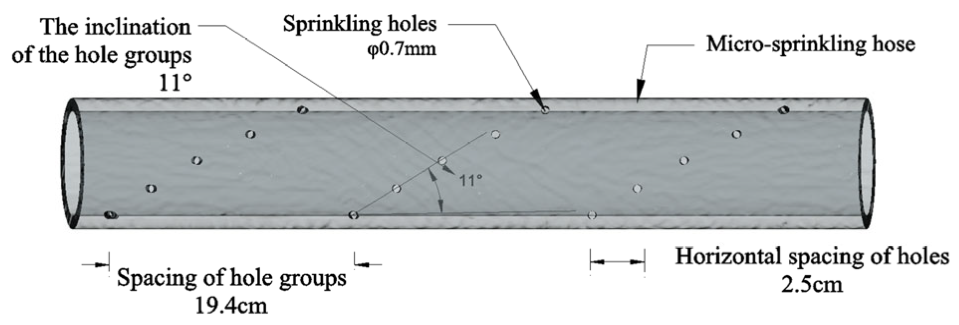
2.1. Materials

The herbicide used in the experiment was quinclorac (C10H5C12N02) (produced by Jiangsu Futian Agrochemical Co. Ltd., Jiangsu Futian, China). Quinclorac is a selective herbicide for controlling barnyard grass in rice fields, and although it is mainly used for controlling barnyard grass, it also has certain control effects on weeds such as Echinochloa oryzoides (Echinochloa phyllopogon (stapf) Koss.), Monochoria (Monochoria korsakowii Regel et Maack), and water fennel (Oenanthe javanica (Blume) DC).

We used microsprinker hoses made of polyethylene (PE). According to the Chinese standards of Agricultural Irrigation Equipment-Microsprinkler Hose (NY/T 1361-2007), the diameter of the microsprinkler hose used was 32 mm with a single row of 5 diagonal holes. Figure 1 shows the physical model of the microsprinkler hose and the main parameter indices used in this study. The horizontal spacing of the holes was 2.5 cm, the spacing of the hole groups was 19.4 cm, the inclination of the hole groups was 11°, the aperture was 0.7 mm, the hose thickness was 0.02 mm, and the work pressure was 55 kPa (produced by Shaanxi Yangling Fengyuan Agricultural Equipment Co. Ltd., Shaanxi Yangling, China).

In addition, according to the Chinese Standards of Agricultural irrigation equipment for water-driven chemical injector pumps (GB/T 19792-2005), an intelligent water, fertilizer, and herbicide integrated application device was produced by our team including a pre-stirring bucket, a stirring bucket, a spraying pump, and a dosing funnel. The pre-stirring bucket was connected to a water source and the stirring bucket through a solenoid valve.

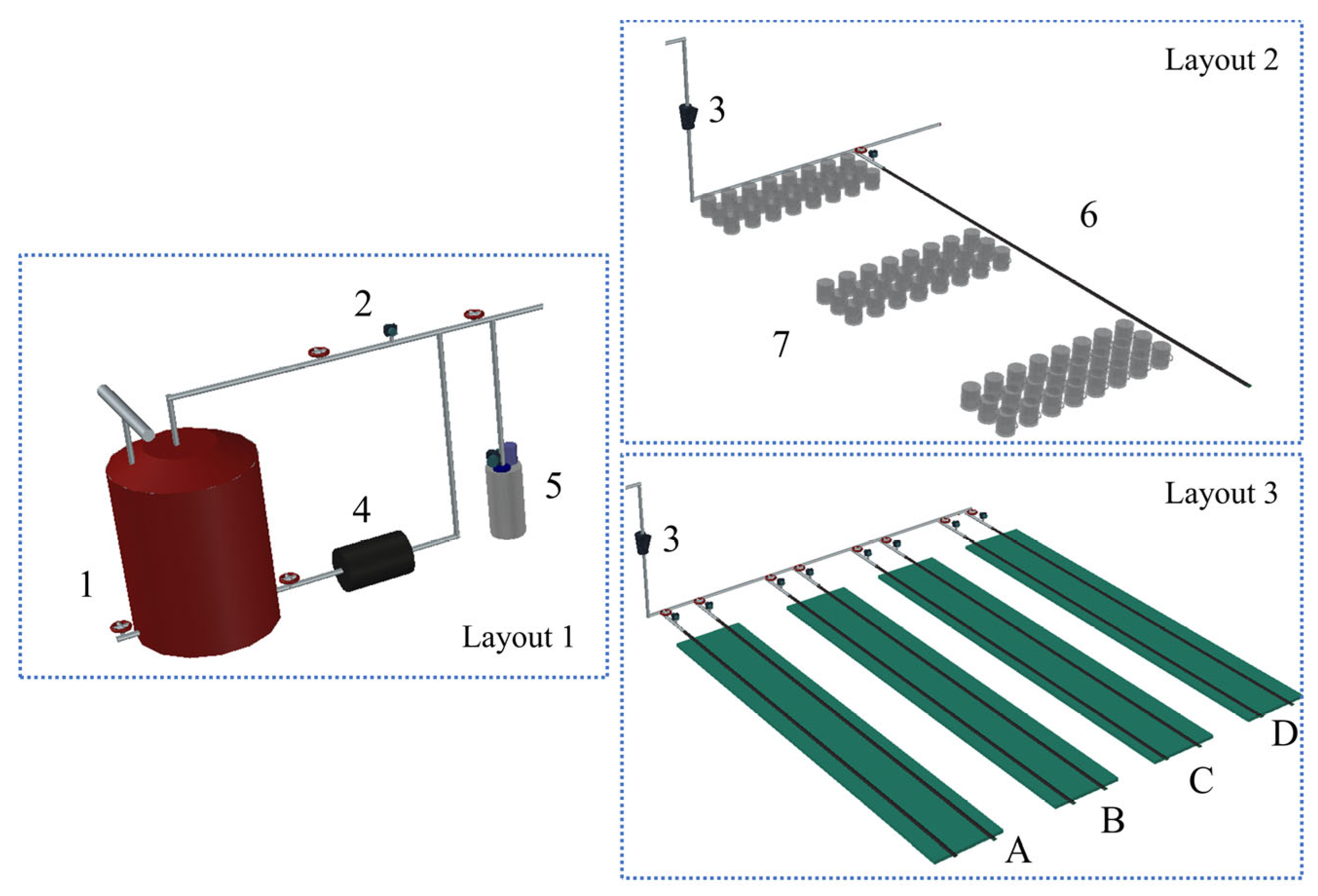
2.2. System Design and Experimental Arrangement

The overall experiment was divided into a water distribution test and an herbicide efficacy experiment. The microsprinkler water flow is the medium for the herbicide to enter the field, so the herbicide distribution is affected by the water distribution. Therefore, the indoor microsprinkler water distribution test was carried out first. After obtaining the water distribution characteristics of the microsprinkler hose, it was necessary to explore and verify the herbicide effect of the microsprinkler application, so an herbicide application field experiment was carried out.

The layout of the experimental system is shown in Figure 2. The laboratory test (Layout 2) and the field experiment (Layout 3) used the same primary pipe system (Layout 1). Both systems were designed according to the Chinese irrigation experimental standard (SL13-2004) and technical code for the micro-irrigation engineering standard (GB/T 50485-2009). The specific test layout and details are described in the next sections.

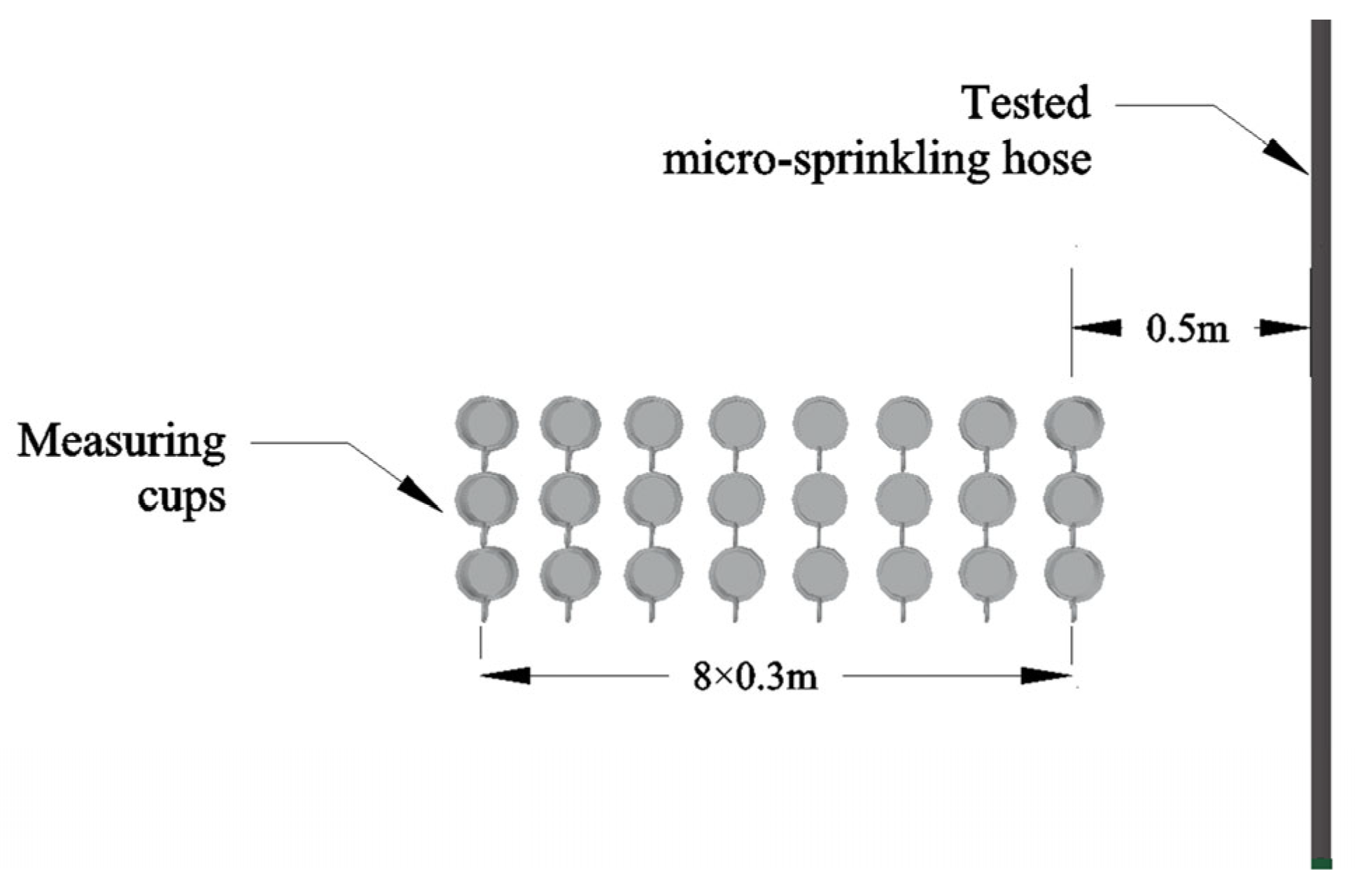
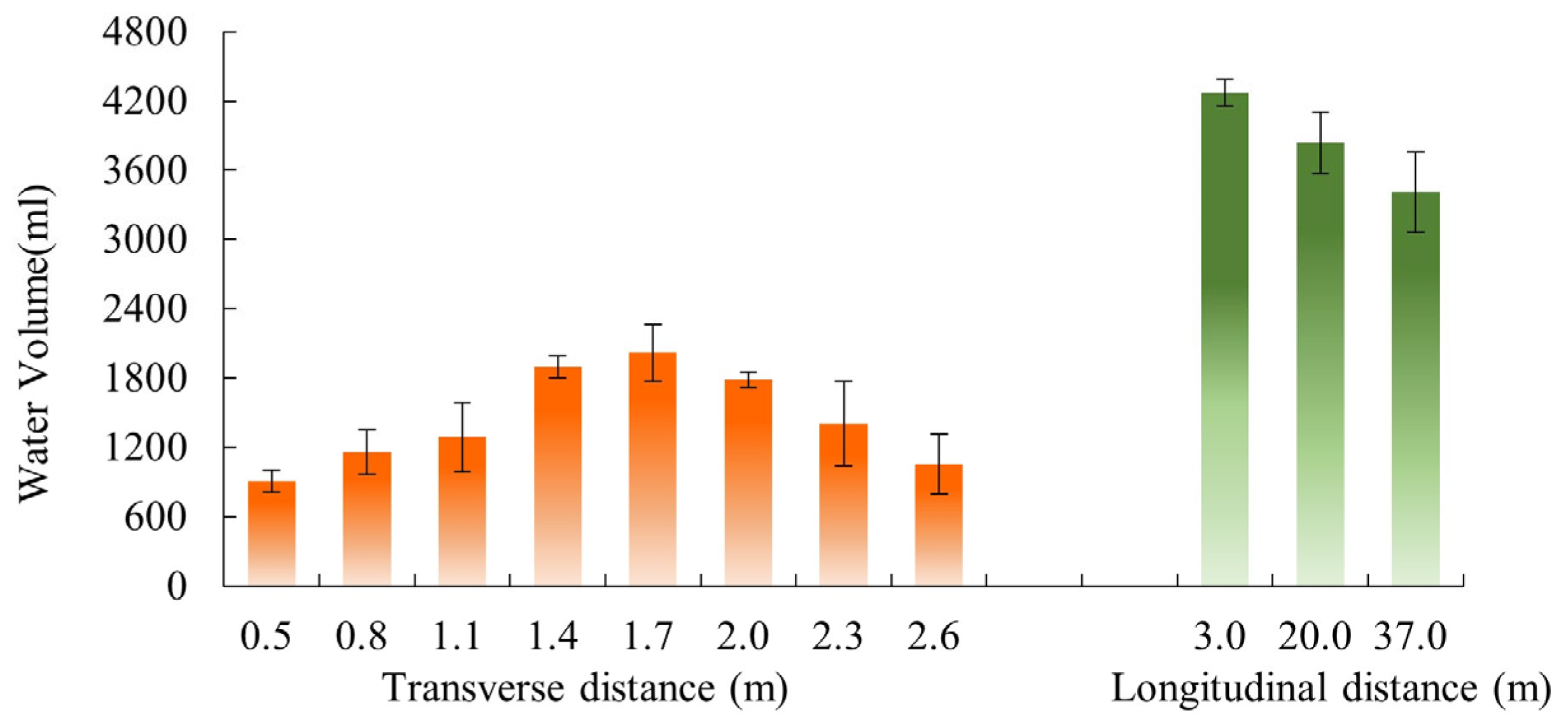
2.2.1. Water Distribution Test

The water distribution test was carried out in the hydraulic laboratory of Northwest Agricultural and Forestry University. The laboratory test consisted of two parts: Layout 1 and Layout 2. The test device consisted of a water storage tank with a mixing function, a water pump, a filter, pressure sensors, pipes, a homemade application device to irrigation, and microsprinkler hoses. The tank was a cylindrical box with a height of 1.55 m and a bottom diameter of 0.745 m. The homemade application device was composed of an application bucket, mixer, and metering pump. The application bucket was a cylindrical plastic bucket with a capacity of 100 L. The flow regulation range of the metering pump was 0–20 L/h, the adjustment gradient was 0.5 L/h, the pressure sensor accuracy was 0.01 kPa, and the measurement range was 0–0.6.

The length of the laid microsprinkler hose was 40 m. The direction along the microsprinkler hose was set as longitudinal, and the direction perpendicular to the microsprinkler hose was set as transverse. The sampling area and measuring cup layout are shown in Figure 3. Sampling points were set at the head (3 m), middle (20 m), and end (37 m) of the transverse direction. The sampling area was started from the microsprinkler hose with a longitudinal distance of 0.5 m. The sampling area of each sampling point was 0.5 m × 2.1 m, and 24 measuring cups were placed in three rows and eight columns to weigh the water volume in the sampling area. The system pressure was set to 55 KPa, and when it was stable, the water amount within 30 min was obtained with measuring cups and repeated three times. The average of the three repeated trials was taken as the final result.

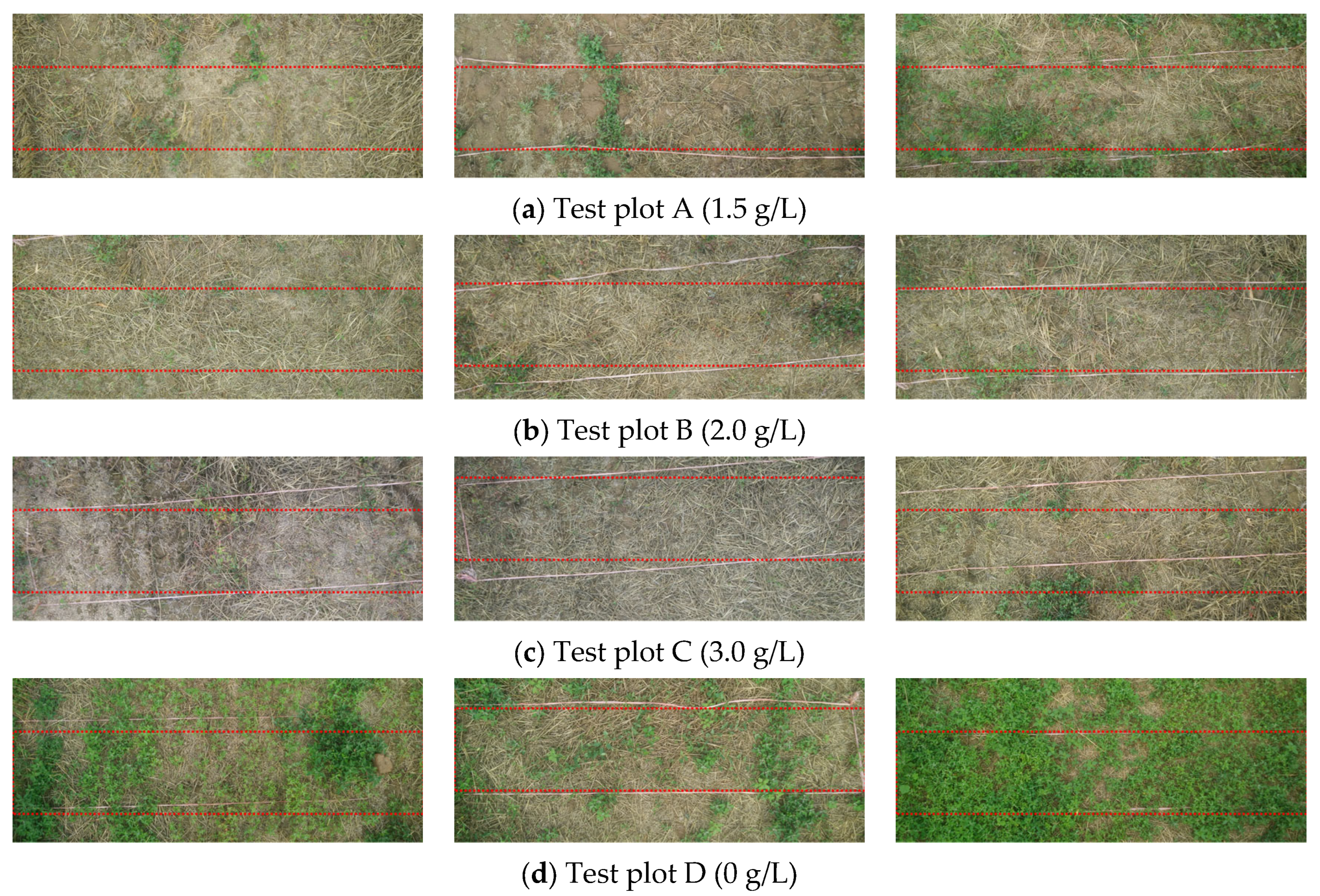
2.2.2. Field Application Experiment

The field experiment was conducted from April 2017 to August 2019 at the Shiyanghe Water-Saving Experimental Station located in Liangzhou, Wuwei, Gansu Province (37°52′ N, 102°50′ E). The field experiment included Layout 1 and Layout 3. In Layout 3, a total of four test plots were set including three test plots (A, B, and C) and one control plot (D). Three field trials were conducted in each plot including two replicates. The test plots were all 40 m in length, 5 m in width, and 200 m² in the control area with buffer zones between the plots. Since the single sprinkle width of the test microsprinkler hose was 2.5 m, each test plot was controlled by two microsprinkler hoses. One hose was used for the herbicide application or water irrigation, and the other hose was used for fertilizer application.

Local weeds in Wuwei include rice barnyard grass (Echinochloa phyllopogon (stapf) Koss. and Echinochloa oryzicola (Vasing.), wild oats (Avena fatua L.), reed (Phragmites australis (Cav.) Trin. ex Steud), goosefoot (Chenopodium album L.), and Sonchus (Sonchus oleraceus L.).

Table 1. Test site and water source.

Parameters	Values
Annual average sunshine hours	3200–3300
Annual average temperature (°C)	8
Frost-free period (day)	150
Annual average rainfall (mm)	164.4
Ions	HCO3−, HSO4−, Cl−, Ca2+, K+, Mg2+
pH	7.3–9.5
Total hardness (mg/L)	200–350
Mineralization (mg/L)	400–600

provides an overview of the experimental site and the water quality of the irrigation water. In this study, the main water source for agricultural irrigation was groundwater, but water resources were relatively scarce and were mainly replenished by precipitation. The test crop was wheat established using machine seeding. The field experiment occurred for three years from 2017 to 2019 including two repeated trials, with sowing in April and harvesting in August. Corn was used as the wheel tillage crop during the field experiments.

During the actual application, quinclorac was weighed and dissolved with water, added to the homemade application device, and then mixed with water in the microsprinkler hose and sprayed onto the field. In the field experiment, herbicide was applied once, and supplemental irrigation (except for natural precipitation) was applied to wheat three times, mainly in three growth stages: the seedling stage, jointing stage, and heading stage. The first irrigation event was carried out after wheat seedling emergence. Before the first irrigation event finished, the herbicide was added to the irrigation water. The herbicide amount was 101.5 g/ha, which is the amount usually used by local farmers. The total herbicide amount applied to each of the four test plots was the same, but different treatment concentrations were applied. The herbicide concentrations in plots A, B, and C were 1.5, 2.0, and 3.0 g/L, respectively, as shown in

Table 2. Treatments and levels.

	Herbicide Content (g)	Water Volume (L)	Concentration (g/L)	Application Duration (s)
Test plot A	30	20	1.5	443
Test plot B	30	15	2.0	332
Test plot C	30	10	3.0	221
Control plot D	0	-	0	-

. It is notable that in test plot D, the irrigation events were the same as in plots A, B, and C, but without herbicide application.

2.3. Evaluation Index and Determination Method

After the experiment, the absolute value survey method (GB/T 17980.47-2000) was used to calculate the weed control effect number in each test plot. Three sampling areas were used at the head, middle, and end of each experimental plot (the distance from the herbicide inlet was 3 m, 20 m, and 37 m, respectively), and five sampling frames were used continuously from each sampling area along the transverse direction. Each sampling frame was 0.5 m long and 0.5 m wide, for a total of 0.25 m². Notably, the defined sampling areas remained fixed during the trial duration. After 8 and 16 days of application, the weeds in the test plots and the control plots were observed to determine whether there were symptoms such as weed drying, yellowing, and wilting or dead spots. After 30 days of application, the wheat was observed for malformations and diseases, and the numbers of dead and living weeds in each sampling frame were counted to calculate the weed control effect.

(1)

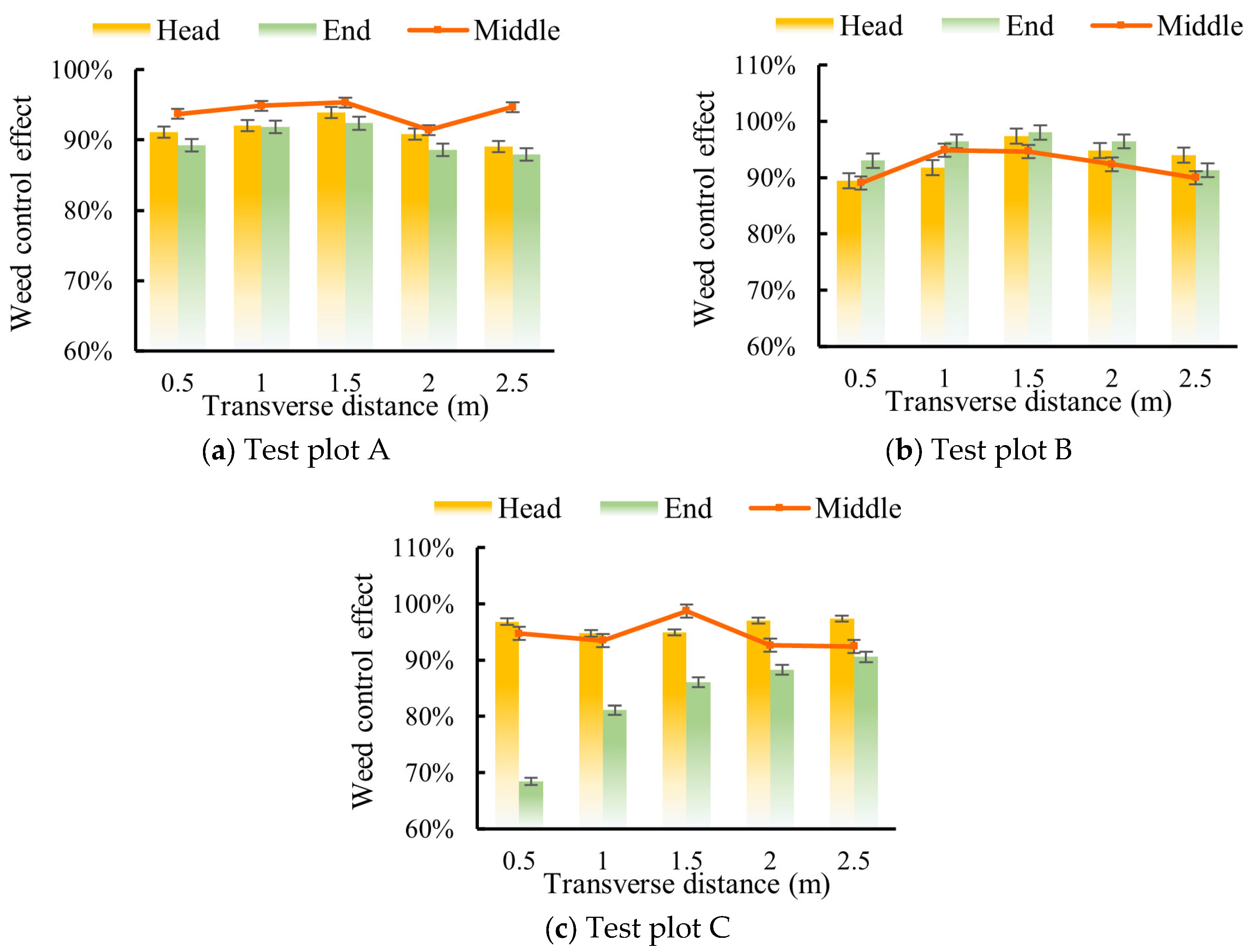
Weed control effect calculation formula [11]:

$$K=\frac{E_{\mathrm{i}}-E_{\mathrm{c}}}{E_{\mathrm{i}}}\times 100\%$$

where K is the weed control effect index; E_i is the number of living weeds in the control plot; E_c is the number of dead weeds in the test plot.

(2)

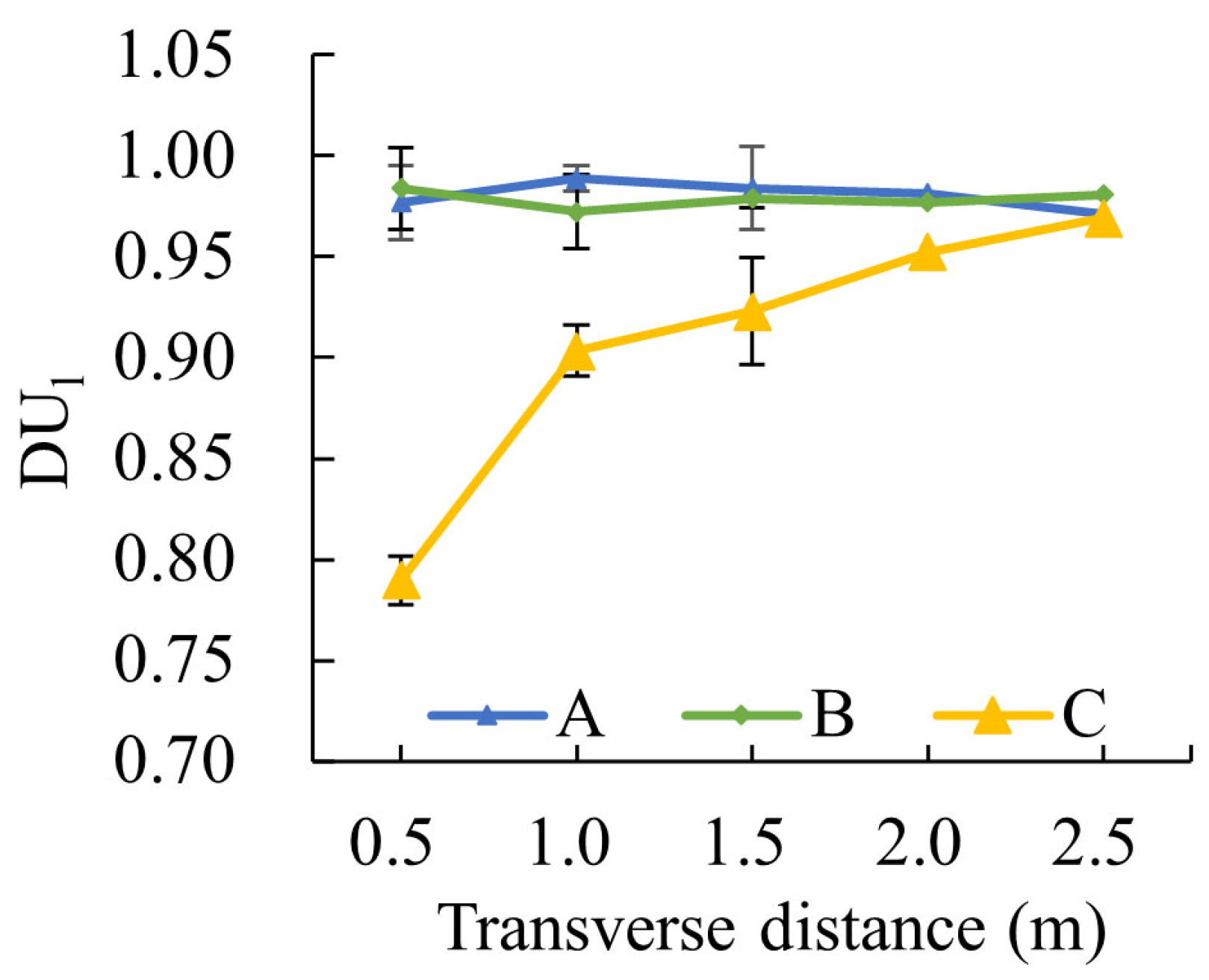
Distribution uniformity coefficient DU: In actual field applications, due to the differences in application devices or artificial uncontrollable factors (the water distribution of microsprinkler hoses is not uniform), the actual amount of herbicide applied in some areas did not reach the amount calculated to achieve optimal application. This index focuses on areas with a low control effect, which is conducive to ensuring the necessary minimum application amount.

$$DU=100\times \frac{\overline{x_i}}{\overline{x}}$$

where DU is the distribution uniformity coefficient; %; $\overline{x_i}$ is the mean K of the observed values in the 1/4 interval with smaller values; and $\overline{x}$ is the mean value of the sample observed values.

The average of the three repetition results was used as the final result. SPSS (version 22.0, IBM Analytics) software was used for statistical analysis. (p = 0.05) was used to determine the significance of the independent variables.

3. Results

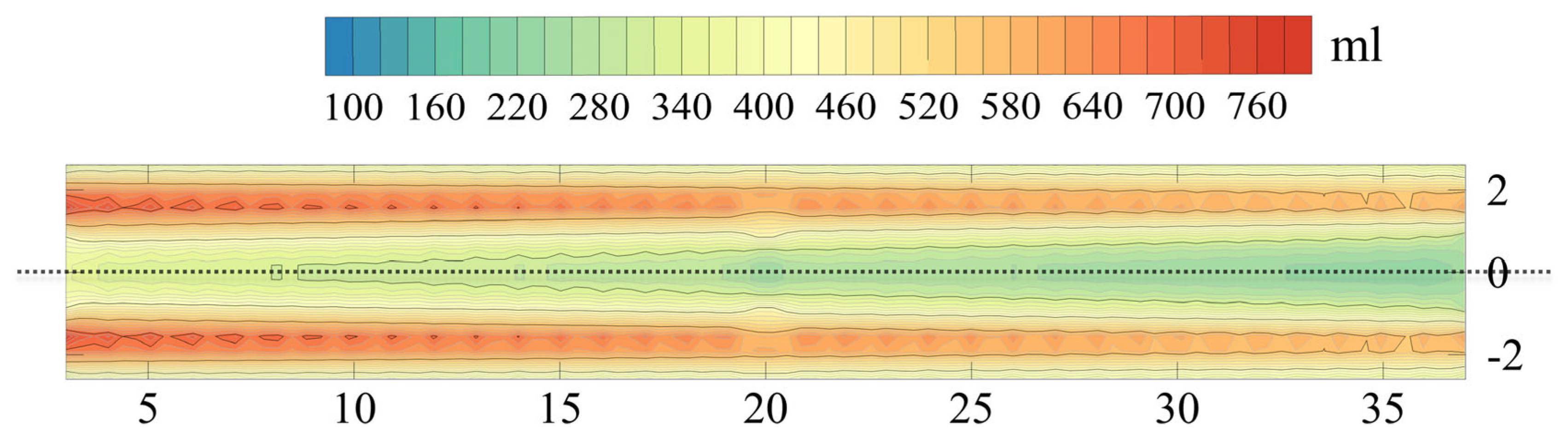
3.1. Water Distribution Characteristics

We tested the cumulative water volume sprayed at different points of the microsprinkler hose to understand the water distribution characteristics and construct (Figure 4). The distribution of the sprayed water in the longitudinal direction was relatively uniform, and the overall water amount was symmetrical along the longitudinal water distribution. There was a point where the sprayed water amount was the maximum, and the diffusion on both sides of the point decreased gradually. The spraying intensity increased first and then decreased gradually in the transverse direction. In the longitudinal direction, the maximum amount of sprayed water volume was 789 mL at 1.7 m away from the microsprinkler hose in the head. At the end of the microsprinkler hose, the maximum water volume was 650 mL at 1.4 m away from the hose. In the middle of the microsprinkler hose, the maximum value was 633 mL at 1.7 m away from the hose.

Figure 5 show the accumulative water amount at each sampling point along the transverse water distribution and the longitudinal water distribution. The accumulative water amount showed a normal distribution. The number of sampling points at the front and back was lower, and the number of sampling points in the middle was higher. The highest water volume was 2018 mL at the sampling point of 1.7 m, and the lowest water volume was 907 mL at the sampling point of 0.5 m. Based on the data comparison, the accumulative water amount at the locations that were 0.5 m, 0.8 m, 1.1 m, 1.4 m, 1.7 m, 2.0 m, 2.3 m, and 2.6 m away from the microsprinkler hose accounted for 7.7%, 7.8%, 9.1%, 19.1%, 17.5%, 16.5%, 12.7%, and 9.6% of the total amount, respectively. This result means that the distribution was not uniform. However, the cumulative water volume of the longitudinal distribution was relatively uniform. The accumulative water amount of the sampling points at 3 m, 20 m, and 37 m was 4270 mL, 3838 mL, and 3409 mL, respectively, which decreased along the hose length gradually, and the amount was the lowest at the last sampling point due to the head loss and pressure drop; this is also an important factor when applying pesticides with microsprinkler irrigation. Due to the long hose and low uniformity, the application effect should be based on the position with the lowest spraying amount, and the spraying duration should be extended to increase the uniformity and meet the requirements of the general pesticide application amount. It is notable that due to the low application amount and short application duration compared with the irrigation water amount, the uneven water distribution had little influence on weed control.

Three repeated trials were conducted during the laboratory experiment to ensure accuracy. The data in Figure 5 are the average values of the three trials. The error bar is the standard error of the three trials.

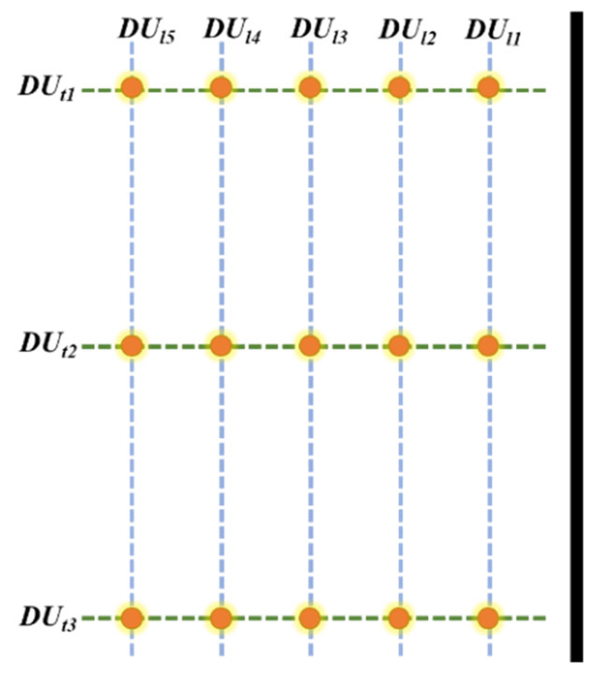
3.2. DU in the Longitudinal and Transverse Directions

On the eighth and sixteenth days following microsprinkler irrigation, the growth of the wheat and weeds in the field was observed, and on the thirtieth day, the dead and live weeds were counted. To facilitate the comparison, we photographed and recorded weed growth at different areas in the three test plots (Figure 6). No malformation, chlorosis, disease spots, or growth retardation were found in the wheat, indicating that the herbicide only had an inhibitory effect on the target weeds and was safe on the wheat crop. Thus, the herbicide application had a significant inhibiting effect on weed growth, ensuring a good growing environment and an adequate nutrient supply for crops. The tested herbicide was not only a feasible option but was also an important factor in ensuring crop growth.

Figure 7 shows the calculated weed control effect after the field experiment and statistical analysis. The value increased first and then decreased in the transverse direction, showing a normal distribution. The highest weed control effect occurred in the middle of the transverse distance, which was related to the water distribution characteristics. In comparison to the other test plots, test plots A and C had the lowest weed control effects. Test plot A had the lowest and highest weed control effects of 87.93% and 95.36%, respectively, with an average of 91.80%. However, the effect in test plot C was lower than that in plot A, at 68.42% and 98.73%, respectively. In fact, due to the higher herbicide concentration, the highest weed control effect in plot C was still higher than that in plot A. However, the overall weed control effect was not high because the effect at the end of the hose was too low. In addition, due to the high concentration, the spraying duration was reduced to maintain the total application amount. A short application duration resulted in the increased influence of the head loss and pressure drop at the end of the hose. According to the water distribution obtained, the cumulative application amount at the end was the lowest, and shortening the application time would have worsened this effect. The overall weed control effect in plot B was higher than that in the other plots. The lowest value was 89.05%, the highest was 98.04%, and the mean was 93.56%. These values were determined by the appropriate herbicide concentration and application duration. Notably, the weed control effect of the sampling point at 37 m was generally lower than that of the other two sampling points, which was obviously related to the water distribution.

Both the 1.5 g/L and 2.0 g/L treatments had better weed control efficiency and generally met the requirements of weed control. Due to the high concentration, the spraying duration was reduced to maintain the total application amount. The short application duration resulted in an increased influence of the head loss and pressure decrease at the end of the hose. At the concentration of 3.0 g/L, the cumulative application amount at the end was too low and did not meet the requirement of stopping weed growth, resulting in poor weed control.

The DUs in the longitudinal (Figure 8) and transverse (Figure 9) directions were calculated according to the weed control effect at different locations.

The data in Figure 9 and Figure 10 are the calculated values of the three trials (2017–2019). The error bar is the standard error of the three trials.

When the concentration was lower than 2.0 g/L, there was little difference in the DUs of the longitudinal distribution at each sampling point maintained above 95%. The longitudinal DU was not significantly different (p > 0.05) along the transverse distance between the sampling points, showing high stability and robustness. However, at a higher concentration (3.0 g/L), the longitudinal DU of each sampling point was significantly different in which the lowest DU (78.9%) and the highest DU (96.9%) even differed by 18%.

The shorter the transverse distance, the lower the longitudinal DU. The longer the transverse distance of the sampling points, the higher the longitudinal DU, and the more uniform the herbicide distribution. Thus, the closer to the microsprinkler hose, the more uneven the herbicide distribution along the hose, which was also reflected in the distribution of the weed control effect and was well explained by the water distribution characteristics. The sampling points with shorter transverse distances received higher amounts of irrigation water, and the difference between the accumulated water and herbicide amount at the front and the end was larger, which aggravated their unevenness. With the increase in the transverse distance, the irrigation water amount decreased, and the difference caused by the irrigation water amount between the head and the end gradually decreased, reducing the influence on the longitudinal DU. In addition, this difference was also due to the shorter application duration. Due to the high herbicide concentration, the application duration needed to be shortened to ensure that the total amount was constant, and the resulting difference also promoted the low longitudinal DU.

Compared with the longitudinal DU, the transverse DU showed minimal differences. The overall trend was slightly different. The longitudinal DU of test plot A was 98.0–98.5%, and the difference was small. The minimum value of test plot B was 96.9–97.1%, which was less than the longitudinal DU of plot A, but the robustness was better. The difference in the DUs of plot C was the largest, the lowest value was 90.2%, and the maximum value was 98.6%. When the treatment concentration was low (1.5 g/L and 2.0 g/L), the transverse DU was consistent with the longitudinal DU, which remained above 95%. The fluctuation was smaller with the increase in longitudinal distance. However, when the treatment concentration was higher (3.0 g/L), the transverse DU gradually decreased with increasing longitudinal distance. Similar to the longitudinal DU, the phenomenon can also be explained by the water consumption distribution. A short application duration, substantial head loss, and decreased irrigation water caused a sudden drop in the transverse DU at the end of the microsprinkler hose.

3.3. Newly Developed Comprehensive DU

The application effect of the microsprinkler hose was tested and compared based on two indices: the weed control effect and weed control uniformity (DU). However, in practical applications, it is tedious and complicated to compare the water distribution and the uniformity of the application effect horizontally and longitudinally. To simplify the description and evaluation of the application uniformity and analyze the influence between the transverse DU and the longitudinal DU, the concept of comprehensive uniformity was introduced according to the comprehensive water distribution uniformity [12]. The relative error of the transverse DU and the longitudinal DU was taken as the evaluation index of the comprehensive uniformity. The smaller the relative deviation, the higher the comprehensive uniformity.

$$\mathit{DU}=1 - \frac{/{\mathit{DU}}_l{-\mathit{DU}}_t/}{{\mathit{DU}}_l}\times 100\%$$

where DU is the comprehensive uniformity; DU_l is the longitudinal uniformity; DU_t is the transverse uniformity.

By combining different measuring points, three transverse DUs and five longitudinal DUs were obtained for each test plot, and 15 comprehensive DUs were obtained by complete combination (Figure 10). The above results were averaged and used to measure the weeding uniformity, as shown in

Table 3. Comprehensive distribution uniformity.

Treatments	Longitudinal Sampling Points (m)	Transverse Sampling Points (m)			Comprehensive DU
		3	20	37
A	0.5	0.992609	0.992288	0.996254	0.994397
	1	0.995442	0.995759	0.99184
	1.5	0.999826	0.999507	0.996555
	2	0.997147	0.996827	0.999225
	2.5	0.986443	0.98612	0.990111
B	0.5	0.985245	0.986992	0.985432	0.991168
	1	0.996892	0.99866	0.997081
	1.5	0.990278	0.992035	0.990467
	2	0.992019	0.993779	0.992208
	2.5	0.988164	0.989917	0.988352
C	0.5	0.750906	0.758269	0.857296	0.921321
	1	0.908547	0.914981	0.998489
	1.5	0.931751	0.938048	0.977263
	2	0.964605	0.970709	0.947207
	2.5	0.982422	0.988421	0.930907

.

The comprehensive DU was consistent with the longitudinal DU and transverse DU. The distribution uniformity of the plots with high concentrations and short application durations was usually lower. The distribution uniformity of the plots with low concentration and long application duration was usually higher. There was no significant difference in the comprehensive distribution uniformity between test plots A and B; that is, the application concentrations of 1.5 g/L and 2.0 g/L both had high weed control uniformity, thus, these concentrations were within the appropriate application concentration range.

4. Discussion

4.1. Application Concentration

The greatest advantage of microsprinkler hoses in the field is that their manufacturing and implementation costs are much lower than those of furrow irrigation; in addition, microsprinkler hoses can be rapidly arranged and recovered, and they not only replenish soil water, but also promote high levels of efficiency and energy savings through the application of fertilizer and water through the application of integrated technology.

According to this paper, microsprinkler use can improve the environment for nutrient competition and enhance growth, which are of great significance to crop growth. In this study, we concluded that the application concentrations of 1.5 g/L and 2.0 g/L both had high weed control uniformity.

However, quinclorac is suitable for paddy transplant fields or seeding fields. Solanaceae (tobacco, potatoes, peppers, etc.), Umbelliferae (carrots and celery), Amarantaceae (spinach and beets), Malvaceae, Cucurbitaceae, Fabaceae crops, and other crops were sensitive to this herbicide [13,14]. Specifically, when spraying in the field, attention should be given to the negative effects on nearby crops [14].

Paddy leaf darkening and curling were mainly caused by excessive quinclorac [15]. Once paddy roots are hypoxic for a long time, a large number of yellow and black roots will appear, leading to a decline in root vitality. After its application, the quinclorac in the paddy did degrade over time, so poisoning symptoms appeared. When applied, it is recommended to use lower herbicide concentrations for a long time or use herbicides several times to prevent damage from the herbicide. Therefore, we believe that 1.5 g/L may be a reasonable concentration for herbicide application with microsprinkler hoses.

4.2. The Cumulative Herbicide Residual

Quinclorac has great mobility in soil and a long residual effect period [2], so it is easy to produce residual pesticide damage to a variety of sensitive crops. If the application of this herbicide exceeds the limit, many aftercrops will incur damage [16]. Watermelon planted after the stubble will appear to be inhibited in growth, dark green leaves, fewer roots, and leaf shrinkage symptoms. Therefore, when paddy fields are changed to plant watermelon and other melon crops [13], attention should be paid to the dose of quinclorac applied in paddy fields and the fine water spray should be increased to reduce the residual amount in the soil to prevent the pesticide damage to the following crops [17]. The content of organic matter in sandy soil is small, and the ability to adsorb herbicides is poor [18]. Therefore, the amount of herbicide should also be appropriately reduced to avoid damaging the root system. Soil with high viscosity and high organic matter content has a strong ability to adsorb herbicides, and the chemical solution cannot easily spread and move in the soil, which can easily cause a massive herbicide layer. When applying the herbicide, the amount can be increased appropriately.

5. Conclusions

Herbicide application with a microsprinkler hose can not only replenish soil moisture, but also achieve high efficiency and energy saving. Through laboratory tests and field irrigation experiments, the water distribution characteristics and the herbicide application effect were explored. The results show that the application effect was correlated with the water distribution characteristics. In general, the lower application concentration (1.5 g/L and 2.0 g/L) had a significantly higher weed control effect and application uniformity than the high concentration treatment (3.0 g/L), which could achieve a better application effect. In practical application, the specific dosage should be determined according to the crop and soil environmental conditions, and the application concentration and duration should be adjusted accordingly.

References

1. Ceng, X.; Li, Y.; Niu, X.; Wang, S. Existing problems and countermeasures in the production, operation, use and management of pesticide in China. Xi’an, Shaanxi, China 2002, 3. Available online: https://kns.cnki.net/kcms/detail/detail.aspx?FileName=IGNE200210001065&DbName=CPFD2002 (accessed on 28 March 2023).
2. Bu, Y.; Kong, Y.; Zhi, Y.; Wang, J.; Dan, Z. Pollution of Chemical Pesticides on Environment and Suggestion for Prevention and Control Countermeasures. J. Agric. Sci. Technol. 2014, 16, 19–25. [Google Scholar]
3. Kavlock, R.J.; Ankley, G.T. A perspective on the risk assessment process for endocrine-disruptive effects on wildlife and human health. Risk Anal. 1996, 16, 731–739. [Google Scholar] [CrossRef] [PubMed]
4. Zhao, H.; Wu, P.; Zhu, D.; Zhang, K.; Feng, Y.; Tan, Z. Spraying Hydraulic Performance of Double Travelling Rain Guns for Hose Reel Irrigator under Low Pressure. Water Sav. Irrig. 2019, 6, 6–9. [Google Scholar]
5. Gao, S.; Li, Q.; Cai, Y.; Bao, L.; Ren, P. Design of Flow Variable Spraying Device. M. Agric. Equip. 2019, 40, 8–42. [Google Scholar]
6. Liu, Y. Solar Power Large Span Translational Administer Sprinkler Design and Test; Anhui Agricultural University: Anhui, China, 2017. [Google Scholar]
7. Hui, X.; Mei, P.; Wang, X. Research of the Detection Method of Indirect ELISA for Acetochlor Residue in Soil. Chem. Bioeng. 2008, 25, 72–74. [Google Scholar]
8. Talaviya, T.; Shah, D.; Patel, N.; Yagnik, H.; Shah, M. Implementation of artificial intelligence in agriculture for optimisation of irrigation and application of pesticides and herbicides. Artif. Intell. Agric. 2020, 4, 58–73. [Google Scholar] [CrossRef]
9. Hura, C.; Leanca, M.; Rusu, L.; Hura, B.A. Risk assessment of pollution with pesticides in food in the Eastern Romania area (1996–1997). Toxicol. Lett. 1999, 107, 103–107. [Google Scholar] [CrossRef] [PubMed]
10. Guo, X.; Feng, Y.; Li, G.; Li, Y.; Zhang, R. Control Efficiency and Safety Evaluation of 3% Foramsulfuron OD on Weeds in Summer Corn Field. J. Shanxi Agric. Sci. 2019, 47, 259–261. [Google Scholar]
11. Gou, W. Experimental Study on Hydraulic Performance of Thin Wall Micro Spray Belt; Tianjin Agricultural University: Tianjing, China, 2019. [Google Scholar]
12. Zhang, G. Dichloroquinolinic acid should not be used in the middle and late period of rice growth. Plant Prot. Technol. Ext. 2002, 1, 29. [Google Scholar]
13. Zhong, Q.; Shen, C.; Chen, R.; Lian, H.; Zhang, Z.; Zhang, J. Effects of three herbicides in rice field on the safety of peanut after stubble. Agric. Technol. 2018, 38, 5–7. [Google Scholar]
14. Liu, Y.; Liu, H.; Zhang, X.; Zhang, W.; Yang, X. Herbicide hazards and their prevention and remediation. Sci. Technol. Tianjin Agric. Forest. 2005, 6, 18–20. [Google Scholar]
15. Ma, H.; Li, G.; Wu, W.; Liu, L. Effects of meteorological factors on herbicide application and application techniques. M. Agric. Sci. Technol. 2006, 5, 77–78. [Google Scholar]
16. Chen, L.; Huang, Y. Cause analysis and prevention and control of herbicide application in maize field. J. Agric. Res. Env. 2012, 29, 23–25. [Google Scholar]
17. He, Y.; Jiang, S.; Shu, X.; Tong, G.; Zhong, M. Research progress on environmental residual status and remediation strategies of quinclorac herbicide. Chin. J. Pestic. Sci. 2021, 23, 31–41. [Google Scholar]
18. Chang, F. Some suggestions for the safe use of herbicides. M. Agric. 2018, 5, 29. [Google Scholar]
Figure 1. Schematic diagram of the microsprinkler hose. The physical model was established, and the main various parameter indices were obtained according to the microsprinkler hose used in the paper.
Agronomy 13 01034 g001
Figure 2. Test system layout. For the purpose of description, the test apparatus and system were divided into three parts. The laboratory test consisted of Layout 1 and Layout 2. The system of field experiment consisted of Layout 1 and Layout 3. 1. water supply tank; 2. pressure sensor; 3. filter; 4. water pump; 5. self-made herbicide application device; 6. untested microsprinkler hose; 7. measuring cups.
Agronomy 13 01034 g002
Figure 3. Sampling area and measuring cup layout. Sampling areas were set at the head (3 m), middle (20 m), and end (37 m) of the transverse direction. Measuring cups in the three sampling areas were arranged in the same way. The figure shows the arrangement of measuring cups in a sampling area.
Agronomy 13 01034 g003
Figure 4. Water distribution of the microsprinkler hose. The figure shows the water distribution. The straight line in the figure is the location of the microsprinkler hose. The abscissa is the longitudinal water distribution (parallel to the direction of the microsprinkler hose), and the ordinate is the transverse water distribution (perpendicular to the direction of the microsprinkler hose).
Agronomy 13 01034 g004
Figure 5. Water accumulation at the transverse sampling points and the longitudinal sampling points.
Agronomy 13 01034 g005
Figure 6. Weeds at the head, middle, and end of the microsprinkler hose in the test plots after 30 days of application. In each test plot, the figures from left to right represent the head, middle, and end of the microsprinkler hose. The picture shows the results of one of the three trials.
Agronomy 13 01034 g006
Figure 7. Weed control effect at the sampling points in the test plots. The data are the average of the three observations. The error bar is the standard error of the observations. After the significance analysis, the intergroup data had significant differences (p ˂ 0.05), while the intragroup data had no significant differences (p ˃ 0.05).
Agronomy 13 01034 g007
Figure 8. Longitudinal distribution uniformity in the test plots.
Agronomy 13 01034 g008
Figure 9. Transverse distribution uniformity in the test plots.
Agronomy 13 01034 g009
Figure 10. Schematic of the comprehensive DU calculation. According to the sampling area, there were three sampling zones in each longitudinal column, five sampling areas in each transverse row, and 15 calculated values were obtained by combining them; these values represent the transverse and longitudinal uniformity of the sample areas, respectively.
Agronomy 13 01034 g010