Climate Projections for Pinot Noir Ripening Potential in the Fort Ross-Seaview, Los Carneros, Petaluma Gap, and Russian River Valley American Viticultural Areas

Abstract

An unbiased MACA CMIP5 ensemble that optimized calculation of the growing season average temperature (GST) viticulture climate classification index throughout Northern California’s Fort Ross-Seaview (FRS), Los Carneros (LC), Petaluma Gap (PG), and Russian River Valley (RRV) American Viticultural Areas (AVAs) was applied to compute the GST index and Pinot noir specific applications of the grapevine sugar ripeness (GSR) model on a mean decadal basis from the 1950s to the 2090s using RCP4.5 and RCP8.5 projections of minimum and maximum daily temperature. From the 1950s to the 2090s, a 2.1/3.6, 2.4/4.2, 2.3/4.0, 2.3/4.0, and 2.3/4.0 °C increase in the GST index and a rate advance of 1.3/1.9, 1.1/1.8, 1.3/2.0, 1.2/1.9, and 1.2/1.9 days a decade was computed for FRS, LC, PG, RRV, and across all four AVAs while using the RCP4.5/RCP8.5 climate projections, respectively. The GST index and GSR model calculations were highly correlated across both climate projections and their fitted models were used to update the Pinot noir specific upper bound for the GST index throughout each AVA using a published optimal harvest window for the northern hemisphere. At a 220 g/L target sugar concentration, the updated upper bound was 17.6, 17.5, 17.6, 17.5, and 17.6 °C for FRS, LC, PG, RRV, and across all four AVAs. For a 240 g/L sugar concentration, it was 17.9, 17.8, 17.9, 17.8, and 17.9 °C. The results from this study together with comparable results recently reported for the Willamette Valley AVA of Oregon using a different downscaled CMIP5 model archive suggest spatial invariance, albeit sugar concentration dependent, for the updated Pinot noir specific upper bound for the GST climate index.

1. Introduction

Grapevine phenology is largely driven by air temperature [1]. Its principal stages, including budburst, flowering, veraison, and maturity have been correlated with various temperature indices [1,2,3,4,5,6,7]. Vitis vinifera L. primarily grows at locations on the globe where growing season average temperatures (GST) range between 12 and 13 °C and 22 and 24 °C [8]. The GST viticulture climate classification index [9], defined as the mean of the observed maximum and minimum daily surface air temperature values from the first of April through the end of October (for the Northern Hemisphere), was correlated with cultivar ripening potential across many wine regions. Various cultivars have their uniquely defined optimal GST value ranges [9]. For example, for optimum suitability of Pinot noir, GST values were originally proposed to range from 14.0 to 16.0 °C, with a high likelihood that changes to the bounds would not exceed 0.6 °C [10,11].

Air temperature also impacts quality for a wine grape growing region [9,12,13]. The rate of decline for total titratable acids (TA), particularly malic acid, during maturation is related to temperature [12]. Better acid retention was observed during ripening for climates with cool nights that accompanied warm days, than climates with warm day and nighttime temperatures [14]. While the primary consequence of a warmer average temperature during ripening was to limit the herbaceous vegetal notes of wines, vintages with high average temperatures were associated with aromas of overripe and cooked fruit [15]. The concentration of anthocyanins in the skins of Pinot noir berries were significantly greater for low (20 °C) relative to high (30 °C) daytime temperatures during ripening, for both low and high light intensities [16]. While Pinot noir coloration was not visually affected by high daytime temperatures (35 °C) for the same nighttime temperature, anthocyanin levels were reduced by 12 to 75 percent relative to Pinot noir fruit ripened at a low daytime temperature (15 °C) [17]. Optimal climate suitability occurs where cultivars ripen at the end of the growing season [12,18]. Several studies have suggested that optimal terroir expression is coincident with a harvest window between 10 September and 10 October (for the Northern Hemisphere) [13,19,20,21].

The impacts of climate change to viticulture have been evaluated using bioclimatic indices and downscaled future climate projections, more recently, for regions in Argentina [22], Bosnia and Herzegovina [23], Europe [24], Greece [3], Italy [25,26], Portugal [27,28], Romania [29], Slovenia [30], and Spain [30,31]. Skahill et al. [32] used localized constructed analogs (LOCA) downscaled Coupled Model Intercomparison Project Phase 5 (CMIP5) daily historic, RCP4.5, and RCP8.5 future datasets [33,34] of minimum and maximum daily surface temperature to spatially compute on a mean decadal basis from the 1950s to the 2090s for Oregon’s Willamette Valley (WV) American Viticultural Area (AVA) the GST index and Pinot noir specific applications of the grapevine sugar ripeness (GSR) model at a 220 g/L target sugar concentration. The grapevine sugar ripeness (GSR) model predicts the day of year to reach fixed target sugar concentrations across sixty-five cultivars [35]. Its development was based on a sequential calibration, sensitivity, and validation exercise using a comprehensive database of target sugar concentrations. It is the linear sum of daily mean temperatures above zero, from the 91st day of the year in the Northern Hemisphere, to an optimized cultivar specific thermal time that is associated with a predetermined sugar concentration level [35].

Using continuous data decomposed into two distinct historical periods (1971–1999; 2000–2012), Van Leeuwen et al. [36] showed that the upper limits of the GST index were underestimated, at least for the Rheingau (Germany, Pinot gris), Burgundy (France, Pinot noir), and Rhone Valley (France, Syrah). Skahill et al. [32] observed a highly correlated one-to-one relationship between the GST index and GSR model calculations throughout the WV AVA using the LOCA CMIP5 datasets and an independent gridded historical meteorological dataset developed for northwestern North America [37]. They used the identified invertible relationship to update the GST bounds for Pinot noir for the WV AVA. The updated bounds corresponded with 10 September and 10 October and were approximately 17.6 and 14.8 °C, respectively. The updated GST bounds indicated that optimal ripening potential for Pinot noir is not only for cool climate, but also intermediate, and slightly warm, climate sub-areas within the WV AVA [38,39]. In cool to intermediate climate regions, high quality vintages were linked to warmer than normal growing seasons for the cultivar Pinot noir [40].

The aim of this study was to apply the methods that were originally used by Skahill et al. [32] for Oregon’s WV AVA to Northern California’s Fort Ross-Seaview, Los Carneros, Petaluma Gap, and Russian River Valley AVAs. This study used the entire twenty-member Multivariate Adaptive Constructed Analogs (MACA) CMIP5 downscaled model archive [41,42] rather than the thirty-two member LOCA CMIP5 model archive that Skahill et al. [32] applied for the WV AVA. The LOCA CMIP5 archive used by Skahill et al. [32] was trained using the Livneh observational dataset [43]. While generally appropriate for most inland areas, the Livneh dataset poorly simulates temperature values in areas of complex terrain such as coastal Northern California due to its application of a fixed lapse rate [43,44]. The MACA CMIP5 model archive used in this study was trained using the Metdata gridded meteorological dataset [45]. The Metdata dataset applies a variable lapse rate and its development closely relied on the Parameter–Elevation Relationships on Independent Slopes Model (PRISM) gridded historical dataset [46] which accounts for the onshore penetration of the marine layer in the coastal zone and cold-air pooling in complex terrain [44]. MACA CMIP5 ensemble selection considered the complete twenty-member MACA CMIP5 archive and was directed to a parsimonious regularized solution [47] that does not overfit the data, which is optimal for computing predictions using future climate projections [48,49,50].

Another aim of this study was to further explore the relationship between calculations of the GST climate index and GSR phenology model, for four Pinot noir producing Northern CA coastal AVAs. To our knowledge, this is the first study to compute projections of the spatiotemporal distribution of the GST index and GSR model for the Fort Ross-Seaview, Los Carneros, Petaluma Gap, and Russian River Valley AVAs. The GST climate index is simple to compute and more accessible for the generalist to apply than the GSR phenology model. The results from this study provide growers and producers with a better understanding of projections for Pinot noir ripening potential in their AVAs. Related, it provides them with the opportunity to pre-emptively begin to evaluate alternate cultivars or plan for shifts regarding winemaking, wine profile, and branding within their AVAs. In addition, by focusing on Pinot noir, results from this study can be compared with those from Skahill et al. [32] regarding projected GST increases, rate advances for ripening, climate suitability for optimal ripening, and updated Pinot noir upper bounds for the GST index. A fundamental question explored in this study was to examine if the one-to-one GSR–GST relationship that was revealed by Skahill et al. [32] for Pinot noir in the WV AVA also exists for the Fort Ross-Seaview, Los Carneros, Petaluma Gap, and Russian River Valley AVAs, and if so, whether the associated updated Pinot noir upper bounds for the GST index are the same or differ by location.

2. Materials and Methods

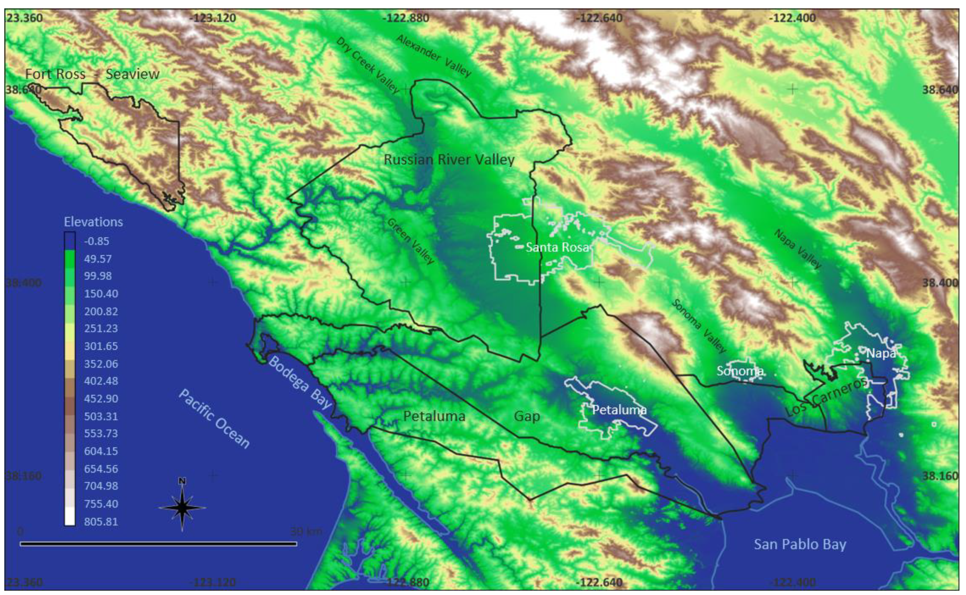
2.1. Study Area

The study area consisted of the Fort Ross-Seaview, Los Carneros, Petaluma Gap, and Russian River Valley AVAs (Figure 1). The boundaries for each of the AVAs and the cities of Napa, Petaluma, Santa Rosa, and Sonoma are shown in Figure 1, including their locations relative to the coastline, Bodega Bay, and San Pablo Bay. The AVA and city boundaries in Figure 1 are overlaid on a digital elevation model for a box region whose extent contains the four AVAs and cities. The four AVAs are nested within California’s North Coast AVA (Figure S1). The Russian River Valley AVA is also nested within the Northern Sonoma AVA (Figure S2). The Fort Ross-Seaview, most of the Russian River Valley, and the sections of the Los Carneros and Petaluma Gap within Sonoma County are all nested within California’s Sonoma Coast AVA (Figure 1 and Figure S3). The land area of the Los Carneros AVA in Napa/Sonoma County is nested within the Napa/Sonoma Valley AVA (Figure 1 and Figure S4).

The final rule by the U.S. Treasury for the establishment of the Fort Ross-Seaview AVA was effective on 13 January 2012 [51]. The AVA has several distinguishing features, including elevation, distance to the coast, and well-drained low fertility soils. Most vineyards within the AVA are planted above the marine fog layer (at elevations between 920 and 1800 feet (≈280–549 m)) and receive longer periods of sunlight and are warmer than the surrounding land area below [51]. Both the fog layer and the nearby ocean moderate temperatures. Approximately 555 acres of grapevine, mostly Pinot noir and Chardonnay, are currently grown in the Fort Ross-Seaview AVA. Plantable acreage within the AVA is limited due to its remote steep mountainous terrain [51]. A median Pinot noir harvest date and wine alcohol content of 23 September and 14.1% was computed from a limited record of Fort Ross-Seaview AVA producer technical data. Pinot noir wine alcohol contents ranged from 13.5% to 14.7% with a mean and standard deviation of 14.05% and 0.4%. The mean harvest date for Pinot noir was 20 September. Its standard deviation was approximately 12 days.

The Los Carneros, or Carneros, AVA was established on September 19, 1983. Soil and climate distinguish the AVA from its surrounding areas [52]. The soils of the AVA are unique relative to the remaining area of the Napa and Sonoma Valley AVAs (Figure 1 and Figure S4). They are cooler, shallower, higher in clay content with lower usable field capacity, less well-drained, and require summertime irrigation [52]. Its proximity to the San Pablo Bay results in cooler temperatures throughout the AVA relative to the rest of the Napa and Sonoma Valley AVAs [52]. Currently, the AVA has approximately 10,040 planted acres. The predominant red and white wine grape cultivars grown in the Carneros AVA are currently Pinot noir and Chardonnay, respectively. A median Pinot noir harvest date and wine alcohol content of 10 September and 14.5% was computed from a limited record of Los Carneros AVA producer technical data. Pinot noir wine alcohol contents ranged from 13.8% to 15.4% with a mean and standard deviation of 14.5% and 0.4%. The mean harvest date for Pinot noir was 6 September. Its standard deviation was approximately 16 days.

The Petaluma Gap AVA was established on 8 January 2018 [53]. While it shares the marine-influenced climate and coastal fog of the Sonoma Coast AVA, its distinct features are its topography and wind speeds [53]. Its topography supports a transport corridor for cool marine air from the Pacific Ocean to the San Pablo Bay that moderates temperatures throughout the AVA, particularly during the mid-to-late afternoon [53]. This corridor is the largest and most unrestricted access point for marine air along the Sonoma and Marin coast [53]. The frequency of afternoon wind speeds greater than or equal to eight miles per hour and their effect in reducing grapevine photosynthesis is the primary distinguishing feature of the Petaluma Gap AVA [53]. Currently, approximately 75% of the more than 4000 acres of grapevines planted in the AVA are Pinot noir. A mean and standard deviation of 14.0% and 0.52%, and a range from 13.3% to 14.9%, were computed from a limited set of alcohol data compiled for Pinot noir wines produced from the AVA. For the Petaluma Gap AVA, harvest dates are reported to be 10 to 14 days later than for its surrounding warmer AVAs [54]. Pinot noir harvest dates collected from a limited set of producers within the AVA yielded a mean harvest date of 20 September with a standard deviation of 8 days.

The Russian River Valley AVA was first established on 21 November 1983 [55]. Since its initial ruling there have been three amendments to expand the AVA [56,57,58]. The initial petition for the AVA emphasized the distinctive “coastal cool” growing climate of the proposed area relative to its warmer neighbors in Alexander Valley, Dry Creek Valley, and Sonoma Valley [55] (Figure 1). The cool climate was attributed to early morning coastal fog intrusions up the Russian River and its tributaries. The most recent petition to expand the AVA, ruled effective December 16, 2011, further mentioned the fog intrusions up the Russian River, but also emphasized the Petaluma Gap as another corridor for the transport of a cooling marine fog layer into the Russian River Valley [58]. Chardonnay and Pinot noir are currently the two most planted cultivars in the AVA. A mean and standard deviation of 14.3% and 0.3%, and a range from 13.8% to 14.8%, were computed from a limited set of technical data compiled for Pinot noir wines produced from the AVA. The mean harvest date for Pinot noir was 12 September. Its standard deviation was approximately 8 days.

2.2. Data

2.2.1. MACA CMIP5

The entire archive of daily Multivariate Adaptive Constructed Analogs (MACA) Coupled Model Intercomparison Project phase 5 (CMIP5) multi-model historic (1950–2005), RCP4.5, and RCP8.5 future (2006–2100) scenario datasets of minimum and maximum surface air temperature was collected from the MACA data portal for the region defined by (37.75° N, 38.75° N) $\times$ (−123.5° E, −122° E) (https://climate.northwestknowledge.net/MACA/data_portal.php (accessed on 3 November 2022)). The 20 models and modelling groups that provided the global climate model data for MACA downscaling are listed in Table S1. This study used the second version of the MACA downscaled CMIP5 model archive that was trained with the observation-based 1/24° (or approximately 4 km) gridded surface meteorological dataset Metdata [45]. The CMIP5 RCP4.5 future scenario dataset is a radiative forcing stabilization scenario that contains most of the scenarios that were assessed in the Intergovernmental Panel on Climate Change’s Fourth Assessment Report [59]. RCP8.5 is CMIP5′s very high baseline scenario that does not include any specific climate mitigation target (RCP8.5) [60]. These two scenarios were used in this study rather than CMIP5′s low forcing level peak and decline mitigation scenario that assumes full participation of all countries to achieve an emission pathway that limits radiative forcing at 2.6 W/m² by 2100 (RCP2.6) [61]. These data were used to compute on a gridded basis the GST index and Pinot noir specific applications of the GSR phenology model for the Fort Ross-Seaview, Los Carneros, Petaluma Gap, and Russian River Valley AVAs from 1950 through the end of the twenty-first century.

2.2.2. MACA CMIP5 Training Dataset: Metdata

Daily maximum and minimum surface air temperature data were collected from the 1/24° (or approximately 4 km) resolution training dataset, Metdata [45], for version two of the MACA CMIP5 archive from the Center for Integrated Data Analytics for the box region (37.75° N, 38.75° N) $\times$ (−123.5° E, −122° E) (https://cida.usgs.gov/thredds/catalog.html?dataset=cida.usgs.gov/thredds/UofIMETDATA (accessed on 3 November 2022)). The Metdata dataset period of record was 1979–2012. The observation-based Metdata gridded surface meteorological dataset combines the subdaily temporal resolution of the second version of the North American Land Data Assimilation System dataset with the spatial climatologies and monthly variability of the Parameter–Elevation Relationships on Independent Slopes Model (PRISM) gridded dataset [45,46,62]. The Metdata dataset supported development of the MACA CMIP5 multi-model ensemble subset that was used to calculate the GST index and Pinot noir specific applications of the GSR model throughout the four AVAs.

2.2.3. Topography Weather Dataset

Daily maximum and minimum surface air temperature data were collected from the 30-arc resolution (or approximately 800 m) observation-based gridded topography weather (TopoWx) dataset for 1950–2005 [63]. As with the Metdata dataset, TopoWx applies a variable lapse rate. It applies a variable lapse rate by leveraging remotely sensed land skin temperature data [63]. The TopoWx data were used as an independent source for comparison with the MACA CMIP5 ensemble subset predictions of the GST index and Pinot noir specific applications of the GSR model throughout the four AVAs for the CMIP5 defined historical period (1950–2005).

2.3. GST Climate Index

The growing season average temperature climate index, GST [9], is defined in Equation (1).

$$\mathrm{GST}=\frac{1}{n}{{\displaystyle \sum }}_{Apr 1}^{Oct 31}\left(T_{max}+T_{min}\right)/2,$$

(1)

where $n=214$, is the number of days for the northern hemisphere growing season, and $T_{max}$ and $T_{min}$ are the maximum and minimum daily surface air temperature data values in °C, respectively. Its associated viticulture climate classifications are listed in

Table 1. Viticulture climate classifications with corresponding values of the growing season average temperature (GST) index [39].

GST
Class Interval (°C)	Class of Viticulture Climate
<13	Too cool
13–15	Cool
15–17	Intermediate
17–19	Warm
19–21	Hot
21–24	Very hot
>24	Too hot

[39].

2.4. GSR Phenology Model

Application of the temperature-based GSR phenology model [35] involves solving the following equation for $t_s$ (Equation (2)):

$${{\displaystyle \sum }}_{t_o=91}^{t_s}{x}_t\ge F^{*},$$

(2)

wherein the daily summation starts on April 1 ($t_o=91$), $x_t$ denote daily mean temperature values greater than zero, and $t_s$ is the day of the year from 1 January which satisfies the inequality for a predetermined thermal summation value, $F^{*}$, that is associated with a cultivar specific fixed sugar concentration level. The Pinot noir specific GSR model sugar concentration and thermal summation values reported by Parker et al. [35] are listed in

Table 2. Grapevine sugar ripeness model thermal summation, $F^{*}$, and sugar concentration values reported by Parker et al. [35] for Pinot noir. Estimates for potential alcohol are listed for each sugar concentration value for three conversion factors, a lower bound (18), upper bound (16.5), and the official European conversion ratio (16.83) [64].

Target Sugar Concentration g/L	$\mathbf{GSR} {\mathit{F}}^{*}$ Value for Pinot Noir	Potential Alcohol (%)
		Lower Bound (18)	European Conversion Ratio (16.83)	Upper Bound (16.5)
170	2695	9.4	10.1	10.3
180	2734	10.0	10.7	10.9
190	2788	10.6	11.3	11.5
200	2838	11.1	11.9	12.1
210	2899	11.7	12.5	12.7
220	2933	12.2	13.1	13.3

, including associated estimates for % potential alcohol [64].

Fit and Extrapolation of Pinot Noir Specific GSR Sugar Concentration and Thermal Summation Values

A global optimization method was applied to fit the Pinot noir specific sugar concentration and thermal summation values listed in Table 2 to an exponential sigmoid function [35,65]. The fitted model was subsequently used to extrapolate thermal summation values for sugar concentrations greater than 220 g/L, the highest sugar concentration value considered by Parker et al. [35].

2.5. MACA CMIP5 Ensemble Subset Selection

In this study we computed a MACA CMIP5 ensemble subset that optimized evaluations of the GST index for 1979–2005 throughout the box region defined by (38.04° N, 38.71° N) $\times$ (−123.42° E, −122.21° E) that contained the Fort Ross-Seaview, Los Carneros, Petaluma Gap, and Russian River Valley AVAs. The specified model was a general linear model without intercept,

$$M={{\displaystyle \sum }}_{i=1}^{20}{w}_i{M}_i,$$

(3)

where $M_i$ and $w_i$ represent the $i$-th MACA CMIP5 model and its assigned non-negative weight, respectively (Equation (3)). The modelling objective was to minimize model-to-measurement misfit using the elastic net penalty [47] configured in the same manner as it was applied in Skahill et al. [48] and Skahill et al. [32].

3. Results and Discussion

3.1. MACA CMIP5 Ensemble Subset Selection

There were 10,476 computed GST climate index values during 1979–2005 for the box region defined by (38.04° N, 38.71° N) $\times$ (−123.42° E, −122.21° E) for the Metdata dataset, the observations, and each of the twenty models from the MACA CMIP5 archive. Table S2 includes three measures that summarized the performance for each individual model from the MACA CMIP5 archive, the MACA CMIP5 ensemble subset obtained from application of the elastic net penalty, and the MACA CMIP5 twenty model ensemble mean. The three measures in Table S2 included the percent bias (PBIAS), the Nash–Sutcliffe efficiency (NSE) [66], and the Kling–Gupta efficiency (KGE) [67] between simulated and observed values. Percent bias measures the average tendency of simulated values to be larger or smaller than their observed counterparts. Its optimal value is zero. Nash–Sutcliffe efficiency values range from minus infinity to one. An NSE value of one indicates a perfect match between the model and its observations. An NSE value of zero indicates that model predictions are as accurate as the mean of the observed data. NSE values less than zero indicate that the mean of the observed data is a better predictor than the model. Kling–Gupta efficiency values range from minus infinity to one. A model is more accurate when its KGE value is closer to one.

The MACA CMIP5 ensemble subset selected from application of the elastic net penalty did not show any bias, whereas each individual model and the ensemble mean all possessed a non-zero bias for prediction of the GST climate index. In addition, the ensemble subset demonstrated greater predictive power relative to each individual model and the ensemble mean as measured by the NSE and KGE values reported in Table S2. The MACA CMIP5 ensemble subset that optimized evaluations of the GST index for 1979–2005 throughout the box region defined by (38.04° N, 38.71° N) $\times$ (−123.42° E, −122.21° E) included nine models: bcc-csm1-1, bcc-csm1-1-m, CCSM4, inmcm4, IPSL-CM5A-MR, MIROC-ESM-CHEM, MIROC-ESM, MRI-CGCM3, and NorESM1-M, with weights of 0.072552423, 0.095689513, 0.076944294, 0.167587718, 0.038177063, 0.001184944, 0.009209387, 0.424841440, and 0.103271605, respectively. These nine models were not the models with the nine greatest NSE or KGE values reported in Table S2. One of the nine models in the ensemble subset, MIROC-ESM, was ranked 19th as measured by either the NSE or KGE values reported in Table S2.

3.2. GST Climate Index

The results reported in this section were all obtained from GST climate index values that were computed using the nine member MACA CMIP5 ensemble subset identified from application of the elastic net penalty. Climate classifications were assigned according to the GST value ranges and associated labels specified in Table 1.

Spatiotemporal Distribution

The spatiotemporal distribution of the GST climate index values, classified according to Table 1, across the four AVAs on a mean decadal basis from the 1950s through the 2090s for the RCP4.5 and RCP8.5 future projections are shown in Figure 2 and Figure 3, respectively. A southward moving front of warmer temperatures from the Dry Creek and Alexander valleys into the Russian River Valley AVA and the Sonoma and Napa valleys into the Los Carneros AVA combined with a westward moving front of warmer GST values from inland towards the coast is observed in both Figure 2 and Figure 3. The noted pattern is more rapid and intense for the RCP8.5 future projection results shown in Figure 3.

The percent distribution of the GST climate index values, classified according to Table 1, within the Fort Ross-Seaview AVA, Los Carneros AVA, Petaluma Gap AVA, Russian River Valley AVA, and across all four AVAs, computed by decade from the 1950s through the 2090s for the RCP4.5/RCP8.5 future scenarios are shown in Figures S5/S6, S7/S8, S9/S10, S11/S12, and S13/S14, respectively. These figures portray a progressive warming trend for each AVA and across all four AVAs for each emission scenario. It is more pronounced for the RCP8.5 scenario projections. For Fort Ross-Seaview, greater than 95% of the AVA would be classified as warm climate by the 2050s/2030s with the RCP4.5/RCP8.5 scenario. For Los Carneros, greater than 95% of the AVA would be classified as hot climate by the 2050s/2040s with the RCP4.5/RCP8.5 scenario. The Petaluma Gap was the only AVA among the four with land area classified as cool climate. However, any land area classified as cool climate was projected to account for less than one percent of the AVA by the 2020s/2010s with the RCP4.5/RCP8.5 scenario. Greater than 85% of the Petaluma Gap AVA would be classified as a warm or hot climate by the 2040s/2030s with the RCP4.5/RCP8.5 scenario. Greater than 99% of the Russian River Valley AVA was classified as a warm or hot climate by the 2000s with the RCP4.5 or RCP8.5 scenario. Greater than 50% of the AVA would be classified as hot climate by the 2070s/2050s with the RCP4.5/RCP8.5 scenario. Across all four AVAs combined, greater than 95% of the total AVA land area would be classified as a warm or hot climate by the 2050s/2040s with the RCP4.5/RCP8.5 scenario.

Table 3. Summary statistics for Northern California’s Fort Ross-Seaview, Los Carneros, Petaluma Gap, and Russian River Valley American Viticultural Areas of computed decadal means from the 1950s through the 2090s of the growing season average temperature (GST) climate index. Historic and RCP4.5 future MACA CMIP5 model datasets and the selected MACA CMIP5 ensemble subset were used to compute the values of the GST index.

	GST Index (°C) (RCP4.5)
	1950s	1960s	1970s	1980s	1990s	2000s	2010s	2020s	2030s	2040s	2050s	2060s	2070s	2080s	2090s
	Fort Ross-Seaview AVA
Min.	14.8	14.8	15.0	15.1	15.2	15.4	15.6	15.8	16.0	16.2	16.4	16.4	16.6	16.8	16.9
1st Qu.	16.0	16.1	16.3	16.3	16.4	16.6	16.8	17.1	17.3	17.4	17.7	17.6	17.9	18.0	18.1
2nd Qu.	16.4	16.4	16.6	16.7	16.8	17.0	17.1	17.4	17.6	17.7	18.0	18.0	18.2	18.4	18.5
3rd Qu.	16.7	16.7	16.9	17.0	17.1	17.3	17.4	17.7	17.9	18.1	18.4	18.3	18.5	18.7	18.8
Max.	17.3	17.3	17.5	17.6	17.7	17.9	18.1	18.4	18.6	18.7	19.0	18.9	19.1	19.3	19.4
	Los Carneros AVA
Min.	17.2	17.2	17.4	17.5	17.7	17.9	17.9	18.2	18.5	18.7	19.1	18.9	19.2	19.4	19.6
1st Qu.	17.6	17.6	17.8	18.0	18.1	18.3	18.3	18.6	18.9	19.1	19.5	19.3	19.6	19.8	20.0
2nd Qu.	17.9	17.9	18.1	18.2	18.4	18.5	18.6	18.9	19.2	19.4	19.7	19.6	19.9	20.1	20.3
3rd Qu.	18.0	18.0	18.3	18.4	18.5	18.7	18.7	19.0	19.3	19.5	19.9	19.7	20.0	20.3	20.4
Max.	18.8	18.8	19.0	19.1	19.2	19.4	19.5	19.8	20.0	20.2	20.6	20.5	20.7	21.0	21.1
	Petaluma Gap AVA
Min.	13.4	13.4	13.6	13.7	13.8	13.9	14.1	14.4	14.6	14.7	15.0	15.0	15.2	15.4	15.5
1st Qu.	16.2	16.2	16.4	16.5	16.7	16.8	16.9	17.2	17.4	17.6	18.0	17.9	18.1	18.3	18.5
2nd Qu.	16.9	16.9	17.1	17.2	17.3	17.5	17.5	17.8	18.1	18.3	18.6	18.5	18.8	19.0	19.2
3rd Qu.	17.3	17.3	17.5	17.6	17.8	17.9	18.0	18.3	18.6	18.7	19.1	19.0	19.2	19.5	19.6
Max.	18.1	18.1	18.3	18.4	18.5	18.7	18.8	19.1	19.3	19.5	19.9	19.8	20.0	20.3	20.4
	Russian River Valley AVA
Min.	16.3	16.3	16.5	16.6	16.7	16.9	17.0	17.3	17.5	17.7	18.0	17.9	18.1	18.3	18.4
1st Qu.	16.9	16.9	17.1	17.2	17.3	17.5	17.6	17.9	18.2	18.3	18.7	18.6	18.8	19.0	19.2
2nd Qu.	17.1	17.1	17.3	17.5	17.6	17.8	17.8	18.1	18.4	18.5	18.9	18.8	19.0	19.3	19.4
3rd Qu.	17.5	17.5	17.8	17.9	18.0	18.2	18.2	18.5	18.8	18.9	19.4	19.2	19.5	19.7	19.9
Max.	18.5	18.6	18.8	18.9	19.0	19.3	19.2	19.6	19.8	20.0	20.5	20.3	20.6	20.9	21.0
	All four AVAs Combined
Min.	13.4	13.4	13.6	13.7	13.8	13.9	14.1	14.4	14.6	14.7	15.0	15.0	15.2	15.4	15.5
1st Qu.	16.6	16.7	16.8	16.9	17.1	17.2	17.3	17.6	17.9	18.0	18.4	18.3	18.5	18.7	18.8
2nd Qu.	17.0	17.1	17.3	17.4	17.5	17.7	17.7	18.0	18.3	18.5	18.8	18.7	19.0	19.2	19.3
3rd Qu.	17.4	17.5	17.7	17.8	17.9	18.1	18.1	18.4	18.7	18.9	19.3	19.1	19.4	19.6	19.8
Max.	18.8	18.8	19.0	19.1	19.2	19.4	19.5	19.8	20.0	20.2	20.6	20.5	20.7	21.0	21.1

and

Table 4. Summary statistics for Northern California’s Fort Ross-Seaview, Los Carneros, Petaluma Gap, and Russian River Valley American Viticultural Areas of computed decadal means from the 1950s through the 2090s of the growing season average temperature (GST) climate index. Historic and RCP8.5 future MACA CMIP5 model datasets and the selected MACA CMIP5 ensemble subset were used to compute the values of the GST index.

	GST Index (°C) (RCP8.5)
	1950s	1960s	1970s	1980s	1990s	2000s	2010s	2020s	2030s	2040s	2050s	2060s	2070s	2080s	2090s
	Fort Ross-Seaview AVA
Min.	14.8	14.8	15.0	15.1	15.2	15.4	15.8	16.0	16.3	16.5	16.9	17.2	17.6	18.0	18.3
1st Qu.	16.0	16.1	16.3	16.3	16.4	16.7	17.0	17.2	17.5	17.8	18.1	18.5	18.9	19.3	19.6
2nd Qu.	16.4	16.4	16.6	16.7	16.8	17.0	17.4	17.6	17.9	18.1	18.5	18.8	19.3	19.7	20.0
3rd Qu.	16.7	16.7	16.9	17.0	17.1	17.3	17.7	17.9	18.2	18.4	18.8	19.1	19.6	20.0	20.3
Max.	17.3	17.3	17.5	17.6	17.7	18.0	18.3	18.5	18.8	19.1	19.4	19.8	20.2	20.6	20.9
	Los Carneros AVA
Min.	17.2	17.2	17.4	17.5	17.7	17.8	18.1	18.3	18.7	19.0	19.4	19.8	20.4	20.9	21.4
1st Qu.	17.6	17.6	17.8	18.0	18.1	18.3	18.5	18.7	19.1	19.4	19.9	20.2	20.9	21.3	21.8
2nd Qu.	17.9	17.9	18.1	18.2	18.4	18.5	18.7	19.0	19.4	19.7	20.1	20.5	21.1	21.5	22.1
3rd Qu.	18.0	18.0	18.3	18.4	18.5	18.7	18.9	19.1	19.5	19.8	20.3	20.6	21.3	21.7	22.2
Max.	18.8	18.8	19.0	19.1	19.2	19.4	19.6	19.9	20.3	20.5	21.0	21.4	22.0	22.4	23.0
	Petaluma Gap AVA
Min.	13.4	13.4	13.6	13.7	13.8	14.0	14.3	14.5	14.8	15.1	15.4	15.8	16.3	16.7	17.0
1st Qu.	16.2	16.2	16.4	16.5	16.7	16.8	17.1	17.3	17.6	17.9	18.3	18.7	19.3	19.7	20.1
2nd Qu.	16.9	16.9	17.1	17.2	17.3	17.5	17.7	18.0	18.3	18.6	19.0	19.4	20.0	20.4	20.9
3rd Qu.	17.3	17.3	17.5	17.6	17.8	17.9	18.2	18.4	18.8	19.0	19.5	19.9	20.5	20.9	21.4
Max.	18.1	18.1	18.3	18.4	18.5	18.7	18.9	19.2	19.5	19.8	20.3	20.6	21.2	21.7	22.2
	Russian River Valley AVA
Min.	16.3	16.3	16.5	16.6	16.7	16.9	17.3	17.5	17.8	18.0	18.4	18.8	19.2	19.6	19.9
1st Qu.	16.9	16.9	17.1	17.2	17.3	17.5	17.8	18.0	18.4	18.7	19.1	19.4	20.0	20.4	20.8
2nd Qu.	17.1	17.1	17.3	17.5	17.6	17.8	18.0	18.2	18.6	18.9	19.3	19.7	20.3	20.7	21.1
3rd Qu.	17.5	17.5	17.8	17.9	18.0	18.1	18.3	18.6	19.0	19.2	19.7	20.1	20.8	21.1	21.7
Max.	18.5	18.6	18.8	18.9	19.0	19.2	19.4	19.6	20.0	20.3	20.8	21.2	22.0	22.3	23.0
	All four AVAs Combined
Min.	13.4	13.4	13.6	13.7	13.8	14.0	14.3	14.5	14.8	15.1	15.4	15.8	16.3	16.7	17.0
1st Qu.	16.6	16.7	16.8	16.9	17.1	17.3	17.5	17.8	18.1	18.4	18.7	19.1	19.6	20.0	20.4
2nd Qu.	17.0	17.1	17.3	17.4	17.5	17.7	17.9	18.2	18.5	18.8	19.2	19.6	20.2	20.6	21.0
3rd Qu.	17.4	17.5	17.7	17.8	17.9	18.1	18.3	18.5	18.9	19.2	19.6	20.0	20.6	21.1	21.6
Max.	18.8	18.8	19.0	19.1	19.2	19.4	19.6	19.9	20.3	20.5	21.0	21.4	22.0	22.4	23.0

list summary statistics, including minima, maxima, and first, second, and third quartiles of the decadal means from the 1950s through the 2090s for the GST climate index [9] values computed for each AVA using the RCP4.5 and RCP8.5 climate projections, respectively. As measured by their reported median values for both emission scenarios, Fort Ross-Seaview was clearly and consistently the coolest AVA while Los Carneros was, in the same manner, the warmest AVA. For both the RCP4.5 and RCP8.5 scenarios, the reported median values for the Petaluma Gap and Russian River Valley each fell approximately in the middle between Fort Ross-Seaview and Los Carneros. Petaluma Gap’s median GST values were consistently slightly lower valued than those calculated for the Russian River Valley. For both emission scenarios, the reported median GST values computed across all four AVAs consistently fell between the median values reported for the Petaluma Gap and the Russian River Valley.

Across all fifteen decades, for both RCP4.5 and RCP8.5, the average difference between the median GST values for the Los Carneros AVA and the Fort Ross-Seaview AVA was 1.6 °C. For the Los Carneros AVA and the Russian River Valley AVA it was 0.8 °C. For the Los Carneros AVA and the Petaluma Gap AVA, the difference was 1.0 °C for RCP4.5 and 1.1 °C for RCP8.5. The average range of the GST values calculated for the Fort Ross-Seaview AVA, Los Carneros AVA, Petaluma Gap AVA, and the Russian River Valley AVA across all fifteen decades, for both RCP4.5 and RCP8.5, was 2.5, 1.6, 4.8, and 2.4 °C, respectively.

A 2.1/3.6, 2.4/4.2, 2.3/4.0, 2.3/4.0, and 2.3/4.0-degree Celsius increase in the GST index median value was computed from the 1950s to the 2090s for the Fort Ross-Seaview AVA, Los Carneros AVA, Petaluma Gap AVA, Russian River Valley AVA, and across all four AVAs while using the RCP4.5/RCP8.5 climate projections. This equates to an approximate 0.14/0.24, 0.16/0.28, 0.15/0.27, 0.15/0.27, and 0.15/0.27 °C increase for the GST index median value by decade for each AVA and their aggregate area for the RCP4.5 and RCP8.5 scenarios, respectively. For RCP4.5, Skahill et al. [32] computed a 3.1-degree Celsius increase in the GST index median value from the 1950s to the 2090s for the WV AVA in Oregon, which equated to an approximate 0.21 °C increase for the GST index median value by decade.

3.3. GSR Phenology Model

The results reported in this section were all obtained from Pinot noir specific applications of the GSR phenology model that were computed using the nine member MACA CMIP5 ensemble subset identified from application of the elastic net penalty.

3.3.1. Fit and Extrapolation of Pinot Noir Specific GSR Sugar Concentration and Thermal Summation Values

The exponential sigmoid fit to the Pinot noir specific sugar concentration and thermal summation values that were reported by Parker et al. [35] (Table 2), including its extrapolation to a sugar concentration of 260 g/L, is shown in Figure 4. The model fit and subsequent extrapolation was performed to support application of the GSR phenology model with a thermal summation value consistent with the reported Pinot noir technical data from the four AVAs (study area). A sugar concentration value of 240 g/L was selected (13.3–14.5% potential alcohol, and 14.3% using the European conversion ratio [64]). The fitted model yielded a thermal summation value of 2987 for a 240 g/L sugar concentration.

3.3.2. Spatiotemporal Distribution

Although the MACA CMIP5 ensemble was developed to optimize calculation of the GST index for a box region that contained the study area’s AVAs, it was deemed reasonable for GSR application given the similarity of the definitions for the GSR phenology model and the GST climate index (Equations (1) and (2)). The GSR model applications performed on a mean decadal basis from the 1950s through the 2090s across all four AVAs at a 240 g/L sugar concentration level resulted in calculated day of year values that covered most of the GST index calculation period from 1 April to 31 October (Equation (1);

Table 5. Summary statistics for Northern California’s Fort Ross-Seaview, Los Carneros, Petaluma Gap, and Russian River Valley American Viticultural Areas of computed decadal means from the 1950s through the 2090s of Pinot noir specific applications of the grapevine sugar ripeness (GSR) model, which predict the day of the year from 1 January to achieve a 240 g/L sugar concentration level. Historic and RCP4.5 future MACA CMIP5 model datasets and the selected MACA CMIP5 ensemble subset were used to compute the values of the GSR phenology model.

	GSR (240 g/L): Pinot noir (Day of year from 1 January) (RCP4.5)
	1950s	1960s	1970s	1980s	1990s	2000s	2010s	2020s	2030s	2040s	2050s	2060s	2070s	2080s	2090s
	Fort Ross-Seaview AVA
Min.	258	257	256	255	255	253	251	250	248	247	245	245	243	242	241
1st Qu.	264	263	262	261	260	259	257	255	253	252	250	250	248	247	246
2nd Qu.	267	266	265	264	263	262	260	258	256	254	252	253	251	250	248
3rd Qu.	271	270	269	268	267	265	263	261	259	258	255	256	254	253	251
Max.	288	287	285	284	283	280	277	275	273	271	269	269	266	265	264
	Los Carneros AVA
Min.	245	245	244	243	242	241	240	239	237	235	233	234	232	231	230
1st Qu.	251	251	250	248	247	246	245	244	242	240	238	239	237	236	234
2nd Qu.	252	252	251	250	249	248	247	245	243	241	239	240	238	237	235
3rd Qu.	255	254	253	252	251	250	249	247	245	243	241	242	240	238	237
Max.	258	258	257	255	254	253	252	250	248	246	244	245	243	241	240
	Petaluma Gap AVA
Min.	251	250	250	248	247	246	245	244	242	240	238	239	237	236	235
1st Qu.	258	257	257	255	254	253	252	250	248	246	244	245	243	242	240
2nd Qu.	262	261	261	259	258	257	256	254	252	250	248	248	246	245	243
3rd Qu.	269	268	267	266	264	263	262	260	258	256	253	254	251	250	249
Max.	310	308	306	304	302	300	297	293	290	288	284	285	282	280	278
	Russian River Valley AVA
Min.	245	245	244	243	242	241	240	239	237	235	233	234	232	231	230
1st Qu.	256	255	254	253	252	250	250	248	246	244	242	243	240	239	238
2nd Qu.	259	259	258	256	255	254	253	251	249	247	245	246	243	242	241
3rd Qu.	261	260	260	258	257	256	254	253	251	249	247	247	245	244	243
Max.	268	267	266	265	264	262	260	259	257	255	253	253	251	250	249
	All four AVAs Combined
Min.	245	245	244	243	242	241	240	239	237	235	233	234	232	231	230
1st Qu.	256	256	255	254	253	251	250	249	247	245	243	243	241	240	239
2nd Qu.	260	259	259	257	256	255	254	252	250	248	246	246	244	243	242
3rd Qu.	264	264	263	261	260	259	257	256	254	252	249	250	248	247	245
Max.	310	308	306	304	302	300	297	293	290	288	284	285	282	280	278

and

Table 6. Summary statistics for Northern California’s Fort Ross-Seaview, Los Carneros, Petaluma Gap, and Russian River Valley American Viticultural Areas of computed decadal means from the 1950s through the 2090s of Pinot noir specific applications of the grapevine sugar ripeness (GSR) model, which predict the day of the year from 1 January to achieve a 240 g/L sugar concentration level. Historic and RCP8.5 future MACA CMIP5 model datasets and the selected MACA CMIP5 ensemble subset were used to compute the values of the GSR phenology model.

	GSR (240 g/L): Pinot noir (Day of year from 1 January) (RCP8.5)
	1950s	1960s	1970s	1980s	1990s	2000s	2010s	2020s	2030s	2040s	2050s	2060s	2070s	2080s	2090s
	Fort Ross-Seaview AVA
Min.	258	257	256	255	255	253	249	248	246	244	242	240	237	234	232
1st Qu.	264	263	262	261	260	258	255	253	251	249	246	244	241	238	236
2nd Qu.	267	266	265	264	263	261	258	256	253	252	249	246	243	240	238
3rd Qu.	271	270	269	268	267	265	261	259	256	255	252	249	246	243	241
Max.	288	287	285	284	283	280	275	272	270	267	264	261	257	253	252
	Los Carneros AVA
Min.	245	245	244	243	242	241	239	238	235	234	231	228	225	223	220
1st Qu.	251	251	250	248	247	247	245	243	240	239	236	233	230	227	225
2nd Qu.	252	252	251	250	249	248	246	244	241	240	236	234	231	228	225
3rd Qu.	255	254	253	252	251	250	248	246	243	241	238	236	232	229	227
Max.	258	258	257	255	254	253	251	249	246	244	241	239	235	232	229
	Petaluma Gap AVA
Min.	251	250	250	248	247	246	245	243	240	239	236	233	230	227	225
1st Qu.	258	257	257	255	254	253	251	249	246	245	241	239	235	232	230
2nd Qu.	262	261	261	259	258	257	255	252	250	248	245	242	239	235	233
3rd Qu.	269	268	267	266	264	263	260	258	255	254	250	247	243	240	237
Max.	310	308	306	304	302	299	294	291	287	284	279	275	270	266	263
	Russian River Valley AVA
Min.	245	245	244	243	242	241	239	238	235	234	231	229	226	223	220
1st Qu.	256	255	254	253	252	251	249	247	244	242	239	236	233	230	227
2nd Qu.	259	259	258	256	255	254	252	250	247	245	242	239	236	233	231
3rd Qu.	261	260	260	258	257	256	253	251	248	247	244	241	238	235	232
Max.	268	267	266	265	264	262	259	257	254	252	249	246	243	240	239
	All four AVAs Combined
Min.	245	245	244	243	242	241	239	238	235	234	231	228	225	223	220
1st Qu.	256	256	255	254	253	251	250	247	245	243	240	237	234	231	228
2nd Qu.	260	259	259	257	256	255	252	250	248	246	243	240	237	234	231
3rd Qu.	264	264	263	261	260	259	256	254	251	250	246	244	240	237	235
Max.	310	308	306	304	302	299	294	291	287	284	279	275	270	266	263

). For RCP4.5/RCP8.5, across all four AVAs and fifteen decades, the minimum and maximum calculated day of year values to achieve a 240 g/L sugar concentration were 230/220 and 310/310 (Table 5 and Table 6), which equated to covering approximately 76-102/72-102 percent of the GST index calculation period.

The GSR-model-computed day of year values to achieve a 240 g/L sugar concentration on a mean decadal basis from the 1950s through the 2090s are shown in Figure 5 and Figure 6 for the RCP4.5 and RCP8.5 climate projections, respectively. In each figure, the area highlighted green is coincident with an optimal harvest window between 10 September and 10 October (for the Northern Hemisphere) [13,19,20,21]. The areas highlighted dark red, deep pink, hot pink, and pink are associated with harvest windows before 1 September, 1–4 September, 4–7 September, and 7–10 September. These four subdivisions were created to account for the mean and standard deviation values that were reported for harvest dates for each of the four AVAs (study area). In each figure, any AVA area highlighted blue coincided with GSR-model-computed day of year values after 10 October.

A southward moving front of decreasing harvest dates into the Russian River Valley AVA and the Los Carneros AVA combined with a westward moving front of decreasing GSR-model-computed day of year values from inland towards the coast is observed in both Figure 5 and Figure 6. The noted pattern is more rapid and intense for the RCP8.5 future projection results shown in Figure 6.

The percent breakdown of the GSR-model-computed day of year values to achieve a 240 g/L sugar concentration within the Fort Ross-Seaview AVA, Los Carneros AVA, Petaluma Gap AVA, Russian River Valley AVA, and across all four AVAs, computed on a decadal basis from the 1950s through the 2090s for the RCP4.5/RCP8.5 future scenarios are shown in Figures S15/S16, S17/S18, S19/S20, S21/S22, and S23/S24, respectively. These figures portray a progressive trend of decreasing area to support an optimal harvest window for each AVA and across all four AVAs for each RCP-emission scenario. It is more pronounced for the RCP8.5 scenario projections. For Fort Ross-Seaview, less than 50% of the AVA would be classified as suitable to support an optimal harvest window by the 2050s/2040s with the RCP4.5/RCP8.5 scenario. For Los Carneros, greater than 50% of the AVA would achieve a 240 g/L sugar concentration before 1 September by the 2030s/2020s with the RCP4.5/RCP8.5 scenario. Less than 50% of the Petaluma Gap AVA would support an optimal harvest window by the 2030s/2020s with the RCP4.5/RCP8.5 scenario. Greater than 90% of the Russian River Valley AVA would achieve a 240 g/L sugar concentration before 10 September by the 2030s/2020s with the RCP4.5/RCP8.5 scenario. Across all four AVAs combined, less than 25% of the total AVA area would be classified as suitable to support an optimal harvest window by the 2050s/2040s with the RCP4.5/RCP8.5 scenario.

Table 5 and Table 6 list summary statistics for each AVA, including minima, maxima, and first, second, and third quartiles, of the decadal means from the 1950s through the 2090s for the GSR-model-computed day of year to achieve a 240 g/L sugar concentration while using the RCP4.5 and RCP8.5 climate projections, respectively. As measured by their reported median values for both emission scenarios, Fort Ross-Seaview was clearly and consistently the AVA with the latest harvest date while Los Carneros was, in the same manner, the AVA with the earliest. For both the RCP4.5 and RCP8.5 scenarios, the reported median values for the Petaluma Gap and Russian River Valley each fell approximately in the middle between Fort Ross-Seaview and Los Carneros. Petaluma Gap’s median GSR-model-computed day of year values were consistently slightly higher valued than those calculated for the Russian River Valley. For both emission scenarios, the reported median GSR-model day of year values computed across all four AVAs consistently fell between the median values reported for the Petaluma Gap and the Russian River Valley.

Across all fifteen decades, for RCP4.5 and RCP8.5, the average difference between the median GSR model computed day of year values for the Fort Ross-Seaview AVA and the Los Carneros AVA was 13.6 and 13.1 days, respectively. For the Petaluma Gap AVA and the Los Carneros AVA, the average difference was 9 days for RCP4.5 and 8.7 days for RCP8.5. For the Russian River Valley AVA and the Los Carneros AVA it was 6.2 and 6 days, respectively.

The difference in the median values of the GSR-model-computed day of year to achieve a 240 g/L sugar concentration from the 1950s to the 2090s was 18.9/28.9, 17.1/27.0, 19.0/29.6, 18.6/28.9, and 18.4/28.7 days for the Fort Ross-Seaview AVA, Los Carneros AVA, Petaluma Gap AVA, Russian River Valley AVA, and across all four AVAs while using the RCP4.5/RCP8.5 climate projections. This equated to an approximate rate advance of 1.3/1.9, 1.1/1.8, 1.3/2.0, 1.2/1.9, and 1.2/1.9 days a decade for each AVA and their aggregate area for the RCP4.5 and RCP8.5 scenarios, respectively. These estimates assume no alteration of training or management system, scion rootstock combination, or seasonal adaptation practices such as manipulating the leaf area to fruit weight ratio would be implemented. For RCP4.5, Skahill et al. [32] computed a rate advance of 2.7 days a decade for the WV AVA in Oregon.

3.3.3. Comparison of Reported Harvest Dates with GSR Model Calculations

For each AVA,

Table 7. For 2010–2019, a summary of limited observed technical data (harvest date and % alcohol) and their associated GSR-model harvest date calculations for a 240 g/L sugar concentration for Northern California’s Fort Ross-Seaview, Los Carneros, Petaluma Gap, and Russian River Valley American Viticultural Areas for the RCP4.5 and RCP8.5 climate projections. The selected MACA CMIP5 ensemble subset was used to compute the values of the GSR phenology model.

AVA	Observations		GSR (240 g/L): RCP4.5/RCP8.5
	Harvest Date	% Alcohol	Mean	Median	Minimum	Maximum
Fort Ross-Seaview	262.5	13.7	260/258	260/258	251/249	277/275
Los Carneros	250	14.5	247/246	247/246	240/239	252/251
Petaluma Gap	259	14.0	258/257	256/255	245/245	297/294
Russian River Valley	255	14.3	252/251	253/252	240/239	260/259

compares summaries of observed Pinot noir harvest dates from 2010 to 2019 with their GSR model simulated counterparts. Across each AVA, the observations were within the simulated bounds obtained for both GSR-modelled climate projections. The observed and GSR-model-simulated harvest date summaries demonstrated a similar pattern in that their values, when ranked, resulted in the same list of AVAs. The harvest date summary rankings from earliest to latest were Los Carneros, Russian River Valley, Petaluma Gap, and Fort Ross-Seaview. In addition, the reported harvest date summaries agreed reasonably well with their simulated counterparts, with the computed measures of central tendency for the GSR-modelled values differing with their corresponding observations by 1–4.5 days. Moreover, a bias was also identified wherein the GSR-model-simulated harvest date summaries consistently predicted a slightly earlier harvest date than their corresponding observations. The results from the limited set of comparisons across the four AVAs potentially suggests that the RCP4.5 climate projection could be an upper bound for the study area. However, that conclusion is uncertain given that it was based on a single decade comparison (i.e., the 2010s) and that the measures of central tendency for the GSR-modelled RCP4.5 and RCP8.5 harvest date summaries for that decade differed at most by two days.

3.4. GSR–GST Relationships

Based on the similarity of the definitions for the GST climate index (Equation (1)) and the GSR phenology model (Equation (2)) and the updated Pinot noir specific bounds for the GST climate index obtained by Skahill et al. [32] from modelling GSR and GST values computed for Oregon’s WV AVA, this study explored whether a Pinot noir specific GSR–GST relationship such as the one identified for the WV AVA also exists for the Fort Ross-Seaview, Los Carneros, Petaluma Gap, and Russian River Valley AVAs. Assuming a highly correlated one-to-one GSR–GST functional relation does exist for each of the four Northern California Pinot noir producing AVAs as it did for the WV AVA, it was also of interest to further learn whether the updated Pinot noir specific upper bound for the GST climate index varied by location. As in Skahill et al. [32], an updated upper bound for the GST climate index was determined using the identified GSR–GST relationships and a published optimal harvest window for the northern hemisphere (10 September–10 October) [13,19,20,21].

For both climate projections, the computed GST climate index values and the day of year values obtained from the Pinot noir specific applications of the GSR phenology model, for either the 220 g/L or 240 g/L target sugar concentration, were highly correlated across each AVA (Table S3). By decade, for each AVA and for either climate projection (RCP4.5 or RCP8.5) or sugar concentration level (220 g/L or 240 g/L), the computed correlation coefficient was consistently less than −0.99 across all 15 decades (Table S3). In addition, the fitted quadratic curves that modelled the observed nonlinear GSR–GST relationship across all fifteen decades for each AVA, all four AVAs combined, and for either projection, were clearly invertible (Figure 7, Figure 8, Figure 9, Figure 10 and Figure 11) in a neighborhood of the day of year that corresponds with 10 September.

Figure 7, Figure 8, Figure 9, Figure 10 and Figure 11 present plots of computed values for both climate projections of the GST index and the GSR model, at a 220 g/L and 240 g/L target sugar concentration, for each AVA and across all four AVAs. The plots also included the quadratic curves, for each climate projection, that were fitted using the computed GST index and GSR model data from all fifteen decades (1950s–2090s). The 220 g/L sugar concentration was also considered in addition to the 240 g/L target level to allow for a comparison of the updated Pinot noir specific upper bounds for the GST climate index for each of the four northern CA AVAs, at that sugar level, with comparable results obtained from Skahill et al. [32] for the WV AVA.

The highly correlated one-to-one GSR–GST relationships that exist for each AVA and across all four AVAs (Table S3; Figure 7, Figure 8, Figure 9, Figure 10 and Figure 11) were combined with a known optimal harvest window (10 September–10 October) to map the phenology data encapsulated in the GSR model (Parker et al., 2020) on to the GST index and update the Pinot noir specific upper bound which is known to be greater than 16 °C but uncertain [36]. The fitted quadratic curves for both climate projections agreed well for each modelled sugar level in a neighborhood of the day of year corresponding to 10 September (Figure 7, Figure 8, Figure 9, Figure 10 and Figure 11). This was the area of interest in each plot given the focus was to determine an updated Pinot noir specific upper bound for the GST climate index for each AVA and across all four AVAs combined. At a 220 g/L target sugar concentration, the updated upper bound was 17.6, 17.5, 17.6, 17.5, and 17.6 °C for the Fort Ross-Seaview AVA, Los Carneros AVA, Petaluma Gap AVA, Russian River Valley AVA, and across all four AVAs. For a 240 g/L sugar concentration, it was 17.9, 17.8, 17.9, 17.8, and 17.9 °C.

The study results indicated that an updated Pinot noir specific upper bound for the GST climate index is sugar-concentration dependent. The updated Pinot noir specific upper bounds for the GST climate index at the 220 g/L target sugar level agreed well with comparable results recently reported upon for Pinot noir in the WV AVA [32]. Their close agreement suggests that the originally reported upon updated upper bound of 17.6 °C for Pinot noir for the GST climate index is spatially invariant. It is notable to mention that the results from this study and the study by Skahill et al. [32] were each performed using two distinct downscaled CMIP5 model archives, the MACA CMIP5 and LOCA CMIP5 archives, respectively. Moreover, spatial invariance for an updated Pinot noir specific upper bound for the GST climate index was also suggested by the results obtained from across the four northern CA AVAs at either sugar level. Additional related studies for other Pinot noir wine grape growing regions are encouraged to further examine results from application of the methodology presented herein to compute a Pinot noir specific updated upper bound for the GST climate index. The approach could be applied for other cultivars. Its application has the potential to expand the originally reported upon set of twenty-one cultivar-specific GST index bounds to the sixty-five cultivars associated with the GSR phenology model [35].

Pinot noir specific applications of the GSR phenology model and the GST climate index were computed on a gridded basis by decade from the 1950s to the 1990s for the four northern CA AVAs using the gridded topography weather (TopoWx) dataset. The GST climate index value corresponding with 10 September was computed from the quadratic model that was fitted to the five decades of GSR model and GST index values that were computed throughout each AVA. The same procedure was performed using the MACA CMIP5 ensemble subset that optimized evaluations of the GST index for 1979–2005 throughout the box region defined by (38.04° N, 38.71° N) $\times$ (−123.42° E, −122.21° E) that contained the Fort Ross-Seaview, Los Carneros, Petaluma Gap, and Russian River Valley AVAs. For the TopoWx dataset, at a 220 g/L target sugar concentration, the updated Pinot noir specific GST index upper bound was 18.0, 18.0, 18.0, and 17.9 °C for the Fort Ross-Seaview AVA, Los Carneros AVA, Petaluma Gap AVA, and the Russian River Valley AVA. For a 240 g/L sugar concentration, it was 18.2, 18.3, 18.3, and 18.2 °C. For the MACA CMIP5 optimal ensemble subset, at a 220 g/L target sugar concentration, the updated Pinot noir specific GST index upper bound was 17.5, 17.5, 17.6, and 17.5 °C for the Fort Ross-Seaview AVA, Los Carneros AVA, Petaluma Gap AVA, and the Russian River Valley AVA. For a 240 g/L sugar concentration, it was 17.8, 17.8, 17.9, and 17.8 °C. For either sugar level, the results obtained using the TopoWx dataset for the 1950s–1990s were biased consistently higher, by 0.4–0.5 °C for each of the AVAs, relative to the comparable results obtained using the MACA CMIP5 ensemble subset. However, they also further confirmed spatial invariance, albeit sugar concentration dependent, for the updated Pinot noir specific upper bound for the GST climate index.

4. Conclusions

This study examined historic and future projections of climate suitability for the cultivar Pinot noir in the Fort Ross-Seaview, Los Carneros, Petaluma Gap, and Russian River Valley AVAs of northern CA. Regardless of the modelled climate projection (RCP4.5 or RCP8.5), Los Carneros, Russian River Valley, Petaluma Gap, and Fort Ross-Seaview consistently ranked as the warmest to coolest based on each AVA’s median GST index values. The medians of the calculated GSR values throughout each AVA demonstrated a similar pattern, with Los Carneros, Russian River Valley, Petaluma Gap, and Fort Ross-Seaview consistently ranked as the earliest to latest AVAs to achieve a 240 g/L sugar concentration. From the 1950s to the 2090s, a 2.1/3.6, 2.4/4.2, 2.3/4.0, 2.3/4.0, and 2.3/4.0 °C increase in the GST index and a rate advance of 1.3/1.9, 1.1/1.8, 1.3/2.0, 1.2/1.9, and 1.2/1.9 days a decade was computed for the Fort Ross-Seaview AVA, Los Carneros AVA, Petaluma Gap AVA, Russian River Valley AVA, and across all four AVAs while using the RCP4.5/RCP8.5 climate projections, respectively. Comparable results were recently obtained and reported upon for Oregon’s Willamette Valley AVA using similar methods [32]. Comparing the computed temperature increases and rate advances from that study with this one suggests the impacts of climate change to be more pronounced for Pinot noir in the WV AVA relative to the four northern CA AVAs.

For each AVA and RCP-emission scenario, there was a progressive trend of decreasing area to support an optimal harvest window (10 September–10 October) for Pinot noir at a 240 g/L target sugar concentration. By the 2050s/2040s, less than 50% of the Fort Ross-Seaview AVA would be suitable to support an optimal harvest window with the RCP4.5/RCP8.5 scenario. Greater than 50% of the Los Carneros AVA would achieve a 240 g/L sugar concentration before 01 September by the 2030s/2020s with the RCP4.5/RCP8.5 scenario. Less than 50% of the Petaluma Gap AVA would support an optimal harvest window by the 2030s/2020s with the RCP4.5/RCP8.5 scenario. Greater than 90% of the Russian River Valley AVA would achieve a 240 g/L sugar concentration before 10 September by the 2030s/2020s with the RCP4.5/RCP8.5 scenario.

Updated Pinot noir specific upper bounds for the GST climate index were consistent across the four AVAs, approximately 17.6 °C for a 220 g/L sugar concentration and 17.9 °C for a 240 g/L sugar concentration. At the 220 g/L sugar concentration, the updated upper bounds were not only consistent across the four AVAs but also with results reported from a previous study for Pinot noir in the Willamette Valley AVA. The updated GST index upper bounds suggest premium Pinot noir can be produced not only for cool climates, but also for intermediate and mildly warm GST viticulture climate classifications.

The methods that were applied in this study for updating the GST climate index upper bound for Pinot noir are applicable for other cultivars. Updated or altogether new GST climate index bounds are possible for up to sixty-five cultivars using methods from this study.

References

1. Malheiro, A.C.; Campos, R.; Fraga, H.; Eiras-Dias, J.; Silvestre, J.; Santos, J.A. Winegrape phenology and temperature relationships in the Lisbon wine region, Portugal. J. Int. Des. Sci. Vigne Vin 2013, 47, 287–299. [Google Scholar] [CrossRef] [Green Version]
2. Cameron, W.; Petrie, P.R.; Barlow, E.; Howell, K.; Jarvis, C.; Fuentes, S. A comparison of the effect of temperature on grapevine phenology between vineyards. OENO One 2021, 55, 301–320. [Google Scholar] [CrossRef]
3. Koufos, G.C.; Mavromatis, T.; Koundouras, S.; Jones, G.V. Adaptive capacity of winegrape varieties cultivated in Greece to climate change: Current trends and future projections. OENO One 2020, 4, 1201–1219. [Google Scholar] [CrossRef]
4. Jarvis, C.; Barlow, E.; Darbyshire, R.; Eckard, R.; Goodwin, I. Relationship between viticultural climatic indices and grape maturity in Australia. Int. J. Biometeorol. 2017, 61, 1849–1862. [Google Scholar] [CrossRef] [PubMed]
5. Bock, A.; Sparks, T.; Estrella, N.; Menzel, A. Changes in the phenology and composition of wine from Franconia, Germany. Clim. Res. 2011, 50, 69–81. [Google Scholar] [CrossRef] [Green Version]
6. Parker, A.; de Cortázar-Atauri, I.; van Leeuwen, C.; Chuine, I. General phenological model to characterise the timing of flowering and veraison of Vitis vinifera L. Aust. J. Grape Wine Res. 2011, 17, 206–216. [Google Scholar] [CrossRef]
7. Tomasi, D.; Jones, G.V.; Giust, M.; Lovat, L.; Gaiotti, F. Grapevine Phenology and Climate Change: Relationships and Trends in the Veneto Region of Italy for 1964–2009. Am. J. Enol. Vitic. 2011, 62, 329–339. [Google Scholar] [CrossRef]
8. Schultz, H.R.; Jones, G.V. Climate Induced Historic and Future Changes in Viticulture. J. Wine Res. 2010, 21, 137–145. [Google Scholar] [CrossRef]
9. Jones, G.V. Climate and terroir: Impacts of climate variability and change on wine. In Fine Wine and Terroir-The Geoscience Perspective, Proceedings of the Geological Society of American Annual Meeting, Seattle, WA, USA, 2 November 2003; Macqueen, R.W., Meinert, L.D., Eds.; Geoscience Canada Reprint Series Number 9; Geological Association of Canada: St. John’s, NL, Canada, 2006; pp. 1–14. [Google Scholar]
10. Jones, G.V.; White, M.A.; Cooper, O.R.; Storchmann, K. Climate change and global wine quality. Clim. Change 2005, 73, 319–343. [Google Scholar] [CrossRef]
11. Jones, G.V. Climate change and the global wine industry. In Proceedings of the Thirteenth Australian Wine Industry Technical Conference, Adelaide, Australia, 28 July–2 August 2007. [Google Scholar]
12. Jackson, D.I.; Lombard, P.B. Environmental and Management Practices Affecting Grape Composition and Wine Quality—A Review. Am. J. Enol. Vitic. 1993, 44, 409–430. Available online: https://www.ajevonline.org/content/44/4/409 (accessed on 3 October 2022). [CrossRef]
13. van Leeuwen, C.; Destrac-Irvine, A.; Dubernet, M.; Duchêne, E.; Gowdy, M.; Marguerit, E.; Pieri, P.; Parker, A.; de Rességuier, L.; Ollat, N. An Update on the Impact of Climate Change in Viticulture and Potential Adaptations. Agronomy 2019, 9, 514. [Google Scholar] [CrossRef] [Green Version]
14. Kliewer, W.M. Berry Composition of Vitis vinifera Cultivars as Influenced by Photo- and Nycto-Temperatures during Maturation. J. Amer. Soc. Hort Sci. 1973, 98, 153–159. [Google Scholar] [CrossRef]
15. Pons, A.; Allamy, L.; Schüttler, A.; Rauhut, D.; Thibon, C.; Darriet, P. What is the expected impact of climate change on wine aroma compounds and their precursors in grape? OENO One 2017, 51, 141–146. [Google Scholar] [CrossRef] [Green Version]
16. Kliewer, W.M. Effect of Day Temperature and Light Intensity on Coloration of Vitis vinifera L. Grapes. J. Amer. Soc. Hort. Sci. 1970, 95, 693–697. [Google Scholar] [CrossRef]
17. Kliewer, W.M.; Torres, R.E. Effect of controlled day and night temperatures on grape coloration. J. Enol. Viticult. 1972, 23, 71–77. [Google Scholar]
18. Deloire, A.; Vaudour, E.; Carey, V.A.; Bonnardot, V.; van Leeuwen, C. Grapevine responses to terroir: A global approach. OENO One 2005, 39, 149–162. [Google Scholar] [CrossRef] [Green Version]
19. van Leeuwen, C.; Seguin, G. The concept of terroir in viticulture. J. Wine Res. 2006, 17, 1–10. [Google Scholar] [CrossRef]
20. van Leeuwen, C. Terroir: The effect of the physical environment on vine growth, grape ripening and wine sensory attributes. In Managing Wine Quality; Reynolds, A.G., Ed.; Woodhead Publishing Series in Food Science, Technology and Nutrition; Woodhead Publishing Limited: Cambridge, UK, 2010; pp. 273–315. [Google Scholar] [CrossRef]
21. Rienth, M.; Lamy, F.; Schoenenberger, P.; Noll, D.; Lorenzini, F.; Viret, O.; Zufferey, V. A vine physiology-based terroir study in the AOC-Lavaux region in Switzerland: This article is published in cooperation with the XIIIth International Terroir Congress November 17-18 2020, Adelaide, Australia. Guest editors: Cassandra Collins and Roberta De Bei. OENO One 2020, 54, 863–880. [Google Scholar] [CrossRef]
22. Cabré, F.; Nuñez, M. Impacts of climate change on viticulture in Argentina. Reg Env. Change 2020, 20, 12. [Google Scholar] [CrossRef]
23. Trbic, G.; Djurdjevic, V.i.; Mandic, M.V.; Ivanisevic, M.; Cupac, R.; Bajic, D.; Zahirovic, E.; Filipovic, D.; Dekic, R.; Popov, T.; et al. The impact of climate change on grapevines in Bosnia and Herzegovina. Euro-Mediterr. J. Environ. Integr. 2021, 6, 4. [Google Scholar] [CrossRef]
24. Cardell, M.F.; Amengual, A.; Romero, R. Future effects of climate change on the suitability of wine grape production across Europe. Reg. Environ. Change 2020, 19, 2299–2310. [Google Scholar] [CrossRef]
25. Teslic, N.; Vujadinovic, M.; Ruml, M.; Ricci, A.; Vukovic, A.; Parpinello, G.P.; Versari, A. Future climatic suitability of the Emilia-Romagna (Italy) region for grape production. Reg. Environ. Change 2019, 19, 599–614. [Google Scholar] [CrossRef]
26. Dal Monte, G.; Labagnara, T.; Cirigliano, P. Agroclimatic evaluation of Val d’Agri (Basilicata, Italy) suitability for grapevine quality: The example of PDO “Terre dell’Alta Val d’Agri” area in a climate change scenario. Ital. J. Agrometeorol. 2019, 3, 3–12. [Google Scholar] [CrossRef]
27. Santos, M.; Fonseca, A.; Fraga, H.; Jones, G.V.; Santos, J.A. Bioclimatic conditions of the Portuguese wine denominations of origin under changing climates. Int. J. Climatol. 2019, 40, 927–941. [Google Scholar] [CrossRef]
28. Blanco-Ward, D.; Ribeiro, A.; Barreales, D.; Castro, J.; Verdial, J.; Feliciano, M.; Viceto, C.; Rocha, A.; Carlos, C.; Silveira, C.; et al. Climate change potential effects on grapevine bioclimatic indices: A case study for the Portuguese demarcated Douro Region (Portugal). BIO Web Conf. 2019, 12, 01013. [Google Scholar] [CrossRef] [Green Version]
29. Irimia, L.M.; Patriche, C.V.; LeRoux, R.; Quénol, H.; Tissot, C.; Sfîcă, L. Projections of Climate Suitability for Wine Production for the Cotnari Wine Region (Romania). Present Environ. Sustain. Dev. 2019, 13, 5–18. [Google Scholar] [CrossRef]
30. Sirnik, I. Spatial-Temporal Analysis of Climate Change Impact on Viticultural Regions Valencia DO and Goriška Brda. Ph.D. Thesis, Universitat Politécnica de Valencia and Université Rennes 2, Universitat Politécnica de Valencia Repository, Valencia, Spain, 2019. Available online: https://riunet.upv.es/bitstream/handle/10251/131695/Sirnik%20-%20Spatial-temporal%20analysis%20of%20climate%20change%20impact%20on%20viticultural%20regions%20Valencia%20DO%20a…pdf?sequence=1 (accessed on 16 February 2020).
31. Sánchez, Y.; Martínez-Graña, A.M.; Santos-Francés, F.; Yenes, M. Index for the calculation of future wine areas according to climate change application to the protected designation of origin “Sierra de Salamanca” (Spain). Ecol. Indic. 2019, 107, 105646. [Google Scholar] [CrossRef]
32. Skahill, B.; Berenguer, B.; Stoll, M. Temperature-based Climate Projections of Pinot noir Suitability in the Willamette Valley American Viticultural Area. OENO One 2022, 56, 209–225. [Google Scholar] [CrossRef]
33. Pierce, D.W.; Cayan, D.R.; Thrasher, B.L. Statistical Downscaling Using Localized Constructed Analogs (LOCA). J. Hydrometeorol. 2015, 15, 2558–2585. [Google Scholar] [CrossRef]
34. Pierce, D.W.; Cayan, D.R.; Maurer, E.P.; Abatzoglou, J.T.; Hegewisch, K.C. Improved bias correction techniques for hydrological simulations of climate change. J. Hydrometeorol. 2015, 16, 2421–2442. [Google Scholar] [CrossRef]
35. Parker, A.K.; García de Cortázar-Atauri, I.; Gény, L.; Spring, J.-L.; Destrac, A.; Schultz, H.; Molitor, D.; Lacombe, T.; Graça, A.; Monamy, C.; et al. Temperature-based grapevine sugar ripeness modelling for a wide range of Vitis vinifera L. cultivars. Agric. For. Meteorol. 2020, 285–286, 107902. [Google Scholar] [CrossRef]
36. van Leeuwen, C.; Schultz, H.R.; Garcia de Cortazar-Atauri, I.; Duchêne, E.; Ollat, N.; Pieri, P.; Bois, B.; Goutouly, J.P.; Quénol, H.; Touzard, J.M.; et al. Why climate change will not dramatically decrease viticultural suitability in main wine-producing areas by 2050. Proc. Natl. Acad. Sci. USA 2013, 110, E3051–E3052. [Google Scholar] [CrossRef] [PubMed] [Green Version]
37. Werner, A.T.; Schnorbus, M.A.; Shrestha, R.R.; Cannon, A.J.; Zwiers, F.W.; Dayon, G.; Anslow, F. A long-term, temporally consistent, gridded daily meteorological dataset for northwestern North America. Sci. Data 2019, 6, 180299. [Google Scholar] [CrossRef] [PubMed] [Green Version]
38. Jones, G.V.; Webb, L.B. Climate Change, Viticulture, and Wine: Challenges and Opportunities. J. Wine Res. 2010, 21, 103–106. [Google Scholar] [CrossRef]
39. Hall, A.; Jones, G.V. Effect of potential atmospheric warming on temperature based indices describing Australian winegrape growing conditions. Aust. J. Grape Wine Res. 2009, 15, 97–119. [Google Scholar] [CrossRef]
40. Blank, M.; Hofmann, M.; Stoll, M. Seasonal differences in Vitis vinifera L. cv. Pinot noir fruit and wine quality in relation to climate. OENO One 2019, 53, 189–203. [Google Scholar] [CrossRef]
41. Abatzoglou, J.T.; Brown, T.J. A comparison of statistical downscaling methods suited for wildfire applications. Int. J. Climatol. 2012, 32, 772–780. [Google Scholar] [CrossRef]
42. MACA Data Portal. Available online: https://climate.northwestknowledge.net/MACA/data_portal.php (accessed on 6 January 2023).
43. Livneh, B.; Rosenberg, E.A.; Lin, C.; Nijissen, B.; Mishra, V.; Andreadis, K.M.; Maurer, E.P.; Lettenmaier, D.P. A long-term hydrologically based dataset of land surface fluxes and states for the conterminous United States: Updates and extensions. J. Clim. 2013, 26, 9384–9392. [Google Scholar] [CrossRef]
44. Walton, D.; Hall, A. An Assessment of High-Resolution Gridded Temperature Datasets over California. J. Clim. 2018, 31, 3789–3810. [Google Scholar] [CrossRef]
45. Abatzoglou, J.T. Development of gridded surface meteorological data for ecological applications and modelling. Int. J. Climatol. 2013, 33, 121–131. [Google Scholar] [CrossRef]
46. Daly, C.; Halbleib, M.; Smith, J.I.; Gibson, W.P.; Doggett, M.K.; Taylor, G.H.; Curtis, J.; Pasteris, P.P. Physiographically sensitive mapping of climatological temperature and precipitation across the conterminous United States. Int. J. Climatol. 2008, 28, 2031–2064. [Google Scholar] [CrossRef]
47. Zou, H.; Hastie, T. Regularization and Variable Selection via the Elastic Net. J. R. Stat. Soc. B 2005, 67, 301–320. [Google Scholar] [CrossRef] [Green Version]
48. Skahill, B.; Berenguer, B.; Stoll, M. Ensembles for Viticulture Climate Classifications of the Willamette Valley Wine Region. Climate 2021, 9, 140. [Google Scholar] [CrossRef]
49. Herger, N.; Abramowitz, G.; Knutti, R.; Angélil, O.; Lehmann, K.; Sanderson, B.M. Selecting a climate model subset to optimise key ensemble properties. Earth Syst. Dynam. 2018, 9, 135–151. [Google Scholar] [CrossRef] [Green Version]
50. Giorgi, F.; Mearns, L.O. Calculation of Average, Uncertainty Range, and Reliability of Regional Climate Changes from AOGCM Simulations via the “Reliability Ensemble Averaging” (REA) Method. J. Clim. 2002, 15, 1141–1158. [Google Scholar] [CrossRef]
51. Treasury Decision TTB-98, Establishment of the Fort Ross-Seaview Viticultural Area, 76 Fed. Reg. 77684. 27 CFR Part 9. 13 January 2012. Available online: https://www.regulations.gov/docket/TTB-2011-0004/document (accessed on 23 November 2022).
52. Treasury Decision ATF-142, Establishment of Los Carneros Viticultural Area, 48 Fed. Reg. 37365. 27 CFR Part 9. 19 September 1983. Available online: https://www.ttb.gov/images/pdfs/Los_Carneros_final_rule.pdf (accessed on 23 November 2022).
53. Treasury Decision TTB-149, Establishment of the Petaluma Gap Viticultural Area and Modification of the North Coast Viticultural Area, 82 Fed. Reg. 57659. 27 CFR Part 9. 8 January 2018. Available online: https://www.regulations.gov/docket/TTB-2016-0009/document (accessed on 23 November 2022).
54. First Harvest for New Petaluma Gap AVA. Available online: https://www.petaluma360.com/article/news/first-harvest-for-new-petaluma-gap-ava/ (accessed on 7 January 2023).
55. Treasury Decision ATF-159, Russian River Valley Viticultural Area, 48 Fed. Reg. 48812. 27 CFR Part 9. 21 November 1983. Available online: https://www.ttb.gov/images/pdfs/Russian_River_Valley_final_rule.pdf (accessed on 23 November 2022).
56. Treasury Decision TTB-7, Expansion of the Russian River Valley Viticultural Area (2002R-421P), 68 Fed. Reg. 67367. 27 CFR Part 9. 2 February 2004. Available online: https://www.ttb.gov/images/pdfs/rrd/ttb_td07.pdf (accessed on 23 November 2022).
57. Treasury Decision TTB-32, Expansion of the Russian River Valley Viticultural Area (2003R-144T), 70 Fed. Reg. 53297. 27 CFR Part 9. 11 October 2005. Available online: https://www.govinfo.gov/content/pkg/FR-2005-09-08/pdf/05-17758.pdf (accessed on 23 November 2022).
58. Treasury Decision TTB-97, Expansions of the Russian River Valley and Northern Sonoma Viticultural Areas (2003R-144T), 76 Fed. Reg. 70866. 27 CFR Part 9. 16 December 2011. Available online: https://www.regulations.gov/docket/TTB-2008-0009/document (accessed on 23 November 2022).
59. Thomson, A.M.; Calvin, K.V.; Smith, S.J.; Kyle, G.P.; Volke, A.; Patel, P.; Delgado-Arias, S.; Bond-Lamberty, B.; Wise, M.A.; Clarke, L.E.; et al. RCP4.5: A pathway for stabilization of radiative forcing by 2100. Clim. Change 2011, 109, 77–94. [Google Scholar] [CrossRef] [Green Version]
60. Riahi, K.; Rao, S.; Krey, V.; Cho, C.; Chirkov, V.; Fischer, G.; Kindermann, G.; Nakicenovic, N.; Rafaj, P. RCP 8.5—A scenario of comparatively high greenhouse gas emissions. Clim. Change 2011, 109, 33–57. [Google Scholar] [CrossRef] [Green Version]
61. van Vuuren, D.P.; Stehfest, E.; den Elzen, M.G.J.; Kram, T.; van Vliet, J.; Deetman, S.; Isaac, M.; Goldewijk, K.K.; Hof, A.; Beltran, A.M.; et al. RCP2.6: Exploring the possibility to keep global mean temperature increase below 2 °C. Clim. Chang。 2011, 109, 95. [Google Scholar] [CrossRef]
62. Xia, Y.; Mitchell, K.; Ek, M.; Sheffield, J.; Cosgrove, B.; Wood, E.; Luo, L.; Alonge, C.; Wei, H.; Meng, J.; et al. Continental-scale water and energy flux analysis and validation for the North American Land Data Assimilation System project phase 2 (NLDAS-2): 1. Intercomparison and application of model products. J. Geophys. Res. 2012, 117, D03109. [Google Scholar] [CrossRef]
63. Oyler, J.W.; Ballantyne, A.; Jencso, K.; Sweet, M.; Running, S.W. Creating a topoclimatic daily air temperature dataset for the conterminous United States using homogenized station data and remotely sensed land skin temperature. Int. J. Climatol. 2015, 35, 2258–2279. [Google Scholar] [CrossRef]
64. Cowey, G. Predicting alcohol levels. Aust. N. Z. Grapegrow. Winemak. 2016, 626, 68. [Google Scholar]
65. Storn, R.; Price, K. Differential Evolution–A Simple and Efficient Heuristic for Global Optimization over Continuous Spaces. J. Glob. Optim. 1997, 11, 341–359. [Google Scholar] [CrossRef]
66. Nash, J.E.; Sutcliffe, J.V. River flow forecasting through conceptual models part I—A discussion of principles. J. Hydrol. 1970, 10, 282–290. [Google Scholar] [CrossRef]
67. Gupta, H.V.; Kling, H.; Yilmaz, K.K.; Martinez, G.F. Decomposition of the mean squared error and NSE performance criteria: Implications for improving hydrological modelling. J. Hydrol. 2009, 377, 80–91. [Google Scholar] [CrossRef] [Green Version]
Figure 1. Boundaries for the Fort Ross-Seaview, Los Carneros, Petaluma Gap, and Russian River Valley American Viticultural Areas (AVAs) (black) and the Northern California cities of Napa, Petaluma, Santa Rosa, and Sonoma (grey) overlaid on a digital elevation model for a box region containing the four AVAs and cities. The Petaluma Gap AVA is subdivided into a Northern (in Sonoma County) and Southern (in Marin County) section. The Los Carneros AVA is subdivided into a Western (in Sonoma County) and Eastern (in Napa County) section. The horizontal axis is in degrees longitude and the vertical axis is in degrees latitude.
Agronomy 13 00696 g001
Figure 2. Decadal mean GST index climate classification throughout Northern California’s Fort Ross-Seaview, Los Carneros, Petaluma Gap, and Russian River Valley American Viticultural Areas from the 1950s through the 2090s. Historic and RCP4.5 future MACA CMIP5 model datasets and the selected MACA CMIP5 ensemble subset were used to compute the values of the GST index.
Agronomy 13 00696 g002
Figure 3. Decadal mean GST index climate classification throughout Northern California’s Fort Ross-Seaview, Los Carneros, Petaluma Gap, and Russian River Valley American Viticultural Areas from the 1950s through the 2090s. Historic and RCP8.5 future MACA CMIP5 model datasets and the selected MACA CMIP5 ensemble subset were used to compute the values of the GST index.
Agronomy 13 00696 g003
Figure 4. Exponential sigmoid fit to the Pinot noir specific sugar concentration and thermal summation values that were reported by Parker et al. [35] (Table 2), including its extrapolation to a sugar concentration of 260 g/L. The estimated thermal sum for a 240 g/L sugar concentration was 2987.
Agronomy 13 00696 g004
Figure 5. Classification of the decadal mean day of year for Pinot noir to reach a 240 g/L sugar concentration level throughout Northern California’s Fort Ross-Seaview, Los Carneros, Petaluma Gap, and Russian River Valley American Viticultural Areas from the 1950s through the 2090s based on application of the grapevine sugar ripeness model using historic and RCP4.5 future MACA CMIP5 model datasets and the selected MACA CMIP5 ensemble subset.
Agronomy 13 00696 g005
Figure 6. Classification of the decadal mean day of year for Pinot noir to reach a 240 g/L sugar concentration level throughout Northern California’s Fort Ross-Seaview, Los Carneros, Petaluma Gap, and Russian River Valley American Viticultural Areas from the 1950s through the 2090s based on application of the grapevine sugar ripeness model using historic and RCP8.5 future MACA CMIP5 model datasets and the selected MACA CMIP5 ensemble subset.
Agronomy 13 00696 g006
Figure 7. For the Fort Ross-Seaview American Viticultural Area, a scatter plot of the decadal mean growing season average temperature (GST) index and the grapevine sugar ripeness (GSR) model day of year from 1 January for Pinot noir to reach a (a) 220 g/L and (b) 240 g/L sugar concentration level. Values were computed for the 1950s, 2020s, and 2090s using historic, RCP4.5, and RCP8.5 future MACA CMIP5 model datasets and the selected MACA CMIP5 ensemble subset. Also shown are the quadratic model fits to the GSR and GST decadal mean calculations across all fifteen decades (1950s–2090s) for the RCP4.5 and RCP8.5 projections, and the fitted model’s GST index values that correspond to 10 September and 10 October (i.e., the dashed lines).
Agronomy 13 00696 g007
Figure 8. For the Los Carneros American Viticultural Area, a scatter plot of the decadal mean growing season average temperature (GST) index and the grapevine sugar ripeness (GSR) model day of year from 1 January for Pinot noir to reach a (a) 220 g/L and (b) 240 g/L sugar concentration level. Values were computed for the 1950s, 2020s, and 2090s using historic, RCP4.5, and RCP8.5 future MACA CMIP5 model datasets and the selected MACA CMIP5 ensemble subset. Also shown are the quadratic model fits to the GSR and GST decadal mean calculations across all fifteen decades (1950s–2090s) for the RCP4.5 and RCP8.5 projections, and the fitted model’s GST index values that correspond to 10 September and 10 October (i.e., the dashed lines).
Agronomy 13 00696 g008
Figure 9. For the Petaluma Gap American Viticultural Area, a scatter plot of the decadal mean growing season average temperature (GST) index and the grapevine sugar ripeness (GSR) model day of year from 1 January for Pinot noir to reach a (a) 220 g/L and (b) 240 g/L sugar concentration level. Values were computed for the 1950s, 2020s, and 2090s using historic, RCP4.5, and RCP8.5 future MACA CMIP5 model datasets and the selected MACA CMIP5 ensemble subset. Also shown are the quadratic model fits to the GSR and GST decadal mean calculations across all fifteen decades (1950s—2090s) for the RCP4.5 and RCP8.5 projections, and the fitted model’s GST index values that correspond to 10 September and 10 October (i.e., the dashed lines).
Agronomy 13 00696 g009
Figure 10. For the Russian River Valley American Viticultural Area, a scatter plot of the decadal mean growing season average temperature (GST) index and the grapevine sugar ripeness (GSR) model day of year from 1 January for Pinot noir to reach a (a) 220 g/L and (b) 240 g/L sugar concentration level. Values were computed for the 1950s, 2020s, and 2090s using historic, RCP4.5, and RCP8.5 future MACA CMIP5 model datasets and the selected MACA CMIP5 ensemble subset. Also shown are the quadratic model fits to the GSR and GST decadal mean calculations across all fifteen decades (1950s–2090s) for the RCP4.5 and RCP8.5 projections, and the fitted model’s GST index values that correspond to 10 September and 10 October (i.e., the dashed lines).
Agronomy 13 00696 g010
Figure 11. For all four American Viticultural Areas combined (Fort Ross-Seaview, Los Carneros, Petaluma Gap, and Russian River Valley), a scatter plot of the decadal mean growing season average temperature (GST) index and the grapevine sugar ripeness (GSR) model day of year from 1 January for Pinot noir to reach a (a) 220 g/L and (b) 240 g/L sugar concentration level. Values were computed for the 1950s, 2020s, and 2090s using historic, RCP4.5, and RCP8.5 future MACA CMIP5 model datasets and the selected MACA CMIP5 ensemble subset. Also shown are the quadratic model fits to the GSR and GST decadal mean calculations across all fifteen decades (1950s–2090s) for the RCP4.5 and RCP8.5 projections, and the fitted model’s GST index values that correspond to 10 September and 10 October (i.e., the dashed lines).
Agronomy 13 00696 g011