Abstract
Climate-smart agriculture involves practices and crop modelling techniques aiming to provide practical answers to meet growers’ demands. For viticulturists, early prediction of harvest dates is critical for the success of cultural practices, which should be based on accurate planning of the annual growing cycle. We developed a modelling tool to assess the sugar concentration levels in the Douro Superior sub-region of the Douro wine region, Portugal. Two main cultivars (cv. Touriga-Nacional and Touriga-Francesa) grown in five locations across this sub-region were studied. Grape berry sugar data, with concentrations between 170 and 230 g L−1, were analyzed for the growing season campaigns, from 2014–2020, as an indicator of grape ripeness conditioned by temperature factors. Field data were collected by ADVID (“Associação Desenvolvimento Da Viticultura Duriense”), a regional winemaker association, and by Sogrape, the leading wine company from Portugal. The “Phenology Modeling Platform” was used for calibrating the model with sigmoid functions. Subsequently, model optimizations were performed to achieve a harmonized model, suitable for all estates. Model performance was assessed through two metrics: root mean square error (RMSE) and the Nash–Sutcliffe coefficient of efficiency (EFF). Both a leave-one-out cross-validation and a validation with an independent dataset (for 1991–2013) were carried out. Overall, our findings demonstrate that the model calibration achieved an average EFF of 0.7 for all estates and sugar levels, with an average RMSE < 6 days. Model validation, at one estate for 15 years, achieved an R2 of 0.93 and an RMSE < 5. These models demonstrate that air temperature has a high predictive potential of sugar ripeness, and ultimately of the harvest dates. These models were then used to build a standalone easy-to-use computer application (GSCM—Grapevine Sugar Concentration Model), which will allow growers to better plan and manage their seasonal activities, thus being a potentially valuable decision support tool in viticulture and oenology.
1. Introduction
New climate conditions are affecting viticulture and the winemaking sector worldwide [1,2], modifying crop spatial distribution [3], development timings [4], agronomic techniques [5], and altering yields and quality [6,7]. From an agronomic viewpoint, climate change over the main viticultural regions in Southern Europe, such as the Douro winegrowing region (Portugal), is driving progressively warmer and drier conditions, increasing air, soil, and canopy temperatures [8,9]. In effect, air temperature is considered the main forcing factor of grapevine phenology [10,11], harvest timings [12,13], solid soluble, and aroma concentration [14,15]. Given the influence of atmospheric variables on this crop, mainly temperature, as well as the projected climate change pathways for the future, it is necessary to develop specific tools to predict the potential response of grapevines. This will promote a more effective decision-making process and help growers maintain their income.
Phenological models enable either planning viticultural practices in the short term (one season) or project the impacts of climate change on the medium-to-long term [16,17,18]. These models allow an improved understanding of the grapevine growing cycle and its behavior under climate change conditions [19]. In the last decades, several models have been developed for this purpose, such as the widely used conventional growing-degree day model, GDD [20]. The sigmoid model [21] tends to be considered one of the most suitable to predict grapevine development phases [13,19], given its relative simplicity and ease of use. The sigmoid model follows a curve that can be used to characterize berry development and sugar accumulation, starting with a rapid increase phase until it reaches a plateau phase, when sugar content stabilizes [22].
Sigmoid models have been applied in several studies to assess phenological timings in different winemaking regions worldwide [23,24,25,26] to model the main grapevine phenological stages, such as budburst (BBCH08), flowering (BBCH60), and veraison (BBCH81). Grapevine harvest is likely the most important event of the annual cycle for growers, though it is considered a pseudo-phenophase, as it depends not only on grapevine ripening, but also on the grower’s decisions. Although grapevine ripening can be a suitable tracer of the potential harvest date, it is considered one of the most difficult periods to simulate, due to the wide range of interactions within the growing cycle [27]. At the end of the growing season, the desired equilibrium between berry acidity and sugar content sets the technological maturity level. Companies decide to harvest based mainly on grape juice sugar concentration, titratable acidity, and pH (technological maturity). Since the grape berry maturity stage is determinant to berry and wine quality, deciding the harvest date accurately is of major concern for the winemaking sector.
Harvest date modelling is then an important resource to plan farming activities and outline commercial strategies. Nonetheless, the harvest date simulation is still incipient, though some efforts are already being undertaken. Suter et al. (2021) [28] quantified key berry sugar accumulation in Bordeaux (France) vineyards and stated that sugar concentration can offer a good indicator of the ripening phase, though they also highlighted the roles of genetic variation and phenotypic plasticity. Parker et al. (2020), using phenological data from various winegrowing regions in Europe, showed the response of the grapevine to temperature in the ripeness stage and created a new GDD-derived model, called “Grapevine Sugar Ripeness”, and a new sigmoid-based model, named “best SIG”. This study laid a path for new, upcoming studies and modelling solutions to accurately simulate sugar concentration dates in different regions and apply them to different grapevine varieties.
The main objective of the present study is to provide new models to reliably predict berry sugar concentration in the Douro Superior/Upper Douro (DS henceforth) wine sub-region. For this purpose, berry sugar concentration data were obtained on certain days of the year (DOY), for 7 years and at five vineyard estates. Sigmoid models were fitted to the observational data at each sugar concentration level (ranging from 170 to 230 g L−1). Models were calibrated and validated using field data from the selected vineyards. Cross-validation and independent validation techniques were applied to improve the model robustness. Optimized sigmoid models were then used to predict the DOY of each sugar concentration level and at each location (concentration/site pairs). Based on the developed models, a new computer application was developed, which may provide growers and stakeholders with an easy-to-use decision-making tool to estimate annual harvest timings. Section 2 will briefly describe the data and methodologies followed herein, while Section 3 is devoted to the presentation of the main results. A discussion of our main findings will be provided in Section 4, while a summary of the conclusions is given in Section 5.
2. Materials and Methods
2.1. Study Region
The DS is a sub-region of the world-famous Douro wine region, a protected designation of origin (PDO) located in Northern Portugal, along the innermost part of Portugal over the course of the Douro River Valley (Figure 1). It is a unique mountainous steep-slope viticultural region, with a singular landscape and environment, allied with century-old viticultural traditions (demarcated and regulated since 1756), and a highly humanized, cultural and evolutive landscape, classified by UNESCO as World Heritage. In this region, viticulture is, by far, the most important socioeconomic sector. For the present study, five vineyard estates (“Quintas”) located in the DS and owned by private wine companies were selected (Figure 1a). For conciseness, the selected vineyard estates are herein designated by the main cultivar grown at each location (TN—Touriga-Nacional, PRT52206; TF—Touriga-Francesa, PRT52205), with numbering from west to east as follows: TN1, TN2, TN3, TF1, and TF2.
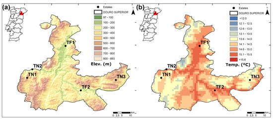
Figure 1.
(a) Elevation (m) map of the Douro Superior (DS) winemaking region and location of the 5 selected vineyard estates (TN1, TN2, TN3, TF1, and TF2). (b) Annual mean temperature (°C) in the DS.
Several climate change impact assessment studies have been carried out over this region, including different grapevine phenological studies [19] and climate change projections on viticultural zoning [6]. Overall, the DS corresponds to the warmest and driest part of the Douro wine region (annual total precipitation of 400–600 mm). This can be explained by the greater distance to the Atlantic Ocean, reinforced by the condensation barrier effect of the surrounding mountains and the relatively low elevations of the valley (from approximately 100 m in the riverbanks up to 600 m at hilltops). The soils are commonly shallow, acid, and dystrophic, derived mainly from old bedrock schist/slate formations of parental material, but also some granite [29], commonly classified as Leptosols, Cambisols, and Anthrosols [30].
The five vineyard estates showed different mean air temperatures (Figure 1b) and were also characterized by different elevations, which underlie different mesoclimates. Digital elevation models combined with climate data (Figure 1b) reveal an approximate temperature range of 3–4 °C from the lower to the upper parts (annual mean temperatures ranging from 12–16 °C). TN1 and TN3 are the coolest estates, with annual mean temperatures of ~14.0 °C, while TF2 (~15.0 °C), TF1, and TN2 (~15.5 °C) are the warmest (Table 1). Overall, the region is characterized by warm temperatures in the growing season (April–October), and sub-humid to semiarid conditions [31]. This is corroborated by the ombrothermic diagram in Figure 2, where the dry season (precipitation lower than 2 times the air temperature) corresponds to the warmest period of the year and extends over four/five months, from May/June to September. Therefore, this dry period extends from the beginning of the grapevine flowering to harvest (Figure 2). During the growing season, warm and dry conditions, with negative soil water balance, are strengthened by the typical “warm soils” that promote early ripeness [32]. Hence, the viticultural and winemaking sector of DS is considered particularly exposed and vulnerable to climate change [3,27].

Table 1.
Characteristics of the 5 vineyard estates, namely: elevation (m), annual mean temperatures (T), and annual precipitation totals (RR) computed over 7 years (2014–2020), along with the total number of phenological observations (Ntot).
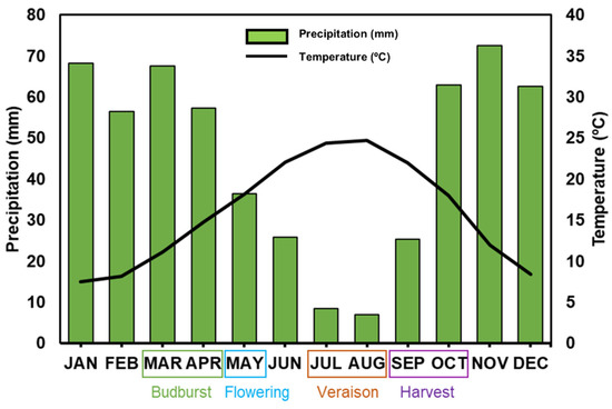
Figure 2.
Ombrothermic diagram according to [33] for the period 2014–2020 and averaged over the five vineyard sites. The typical timings of the mean phenological events in the DS are also highlighted (boxes in the x-axis).
2.2. Datasets
In the context of the CoaClimateRisk project (http://coaclimaterisk.utad.pt (accessed on 29 January 2022)), a 2014–2020 dataset was obtained from ADVID— “Associação Desenvolvimento Da Viticultura Duriense”, and Sogrape, partners of the mentioned project. These datasets include grapevine phenological timings and grape berry quality parameters, systematically collected over the years for two cultivars of Vitis vinifera L.: Touriga-Nacional (TN) and Touriga-Francesa (TF). Although one estate has a longer time series (1991–2020), this dataset was split to obtain calibration (2014–2020) and validation (1991–2013) periods. Both field and laboratory data were recorded always following the same protocols and were subject to quality-checking and homogenization procedures.
Grapevine phenological data were recorded in the five estates using the BBCH scale [34] as a reference, namely the DOY of the main grapevine phenological stages, i.e., budburst (BBCH08), flowering (BBCH60), veraison (BBCH81), and harvest (BBCH89). For measurement purposes, each stage was considered attained when 50% of the grapevines achieved it. To determine harvest, however, the technological maturity was considered, which depends on several oenological/chemical factors, such as sugar level, pH, and total acidity, as well as other human factors, such as sample tasting.
For grape berry ripening monitoring, field samplings of 200 berries from each estate, randomly collected from the different pre-defined reference plots, were taken [35]. Data collection frequency usually ranged from 5 to 10 days. After the berries were collected and weighed, they were crushed using a pneumatic press (Agro-Moderna hydraulic grape pressing machine, 1040 cm3), and the samples of grape juice were subjected to laboratory analysis. Grape berry maturity control consisted of the determination of different parameters, such as potential alcohol, total acidity, and pH, which was carried out in certified laboratories following standard techniques and protocols [36]. A digital refractometer (HANNA Inst. HI996813, Woonsocket, Rhode Island, USA) was used to determine the total soluble solids, equivalent to the potential alcohol content, and subsequently converted into sugar concentration (g L−1). These data were first screened for possible methodological errors, and outliers were removed (either lower than the 5% percentile or higher than the 95% percentile). The final result is the simple arithmetic mean of the readings from each estate [36].
The present study aimed at analyzing sugar concentration in grapevines at the following levels: 170, 180, 190, 200, 210, 220, and 230 g L−1. These levels of sugar concentration were selected based on the methodology proposed by Parker et al. (2020). However, the obtained datasets do not contain the sugar concentration at these very specific levels, since field observations were not carried out daily. Therefore, to estimate the DOY of these fixed levels, a statistical approach was first applied to the time series. Hence, for each year and for each estate, a sugar content curve was estimated using the best adjusted polynomial regression. The 1st or 2nd order polynomial functions were manually selected aiming at both minimizing the quadratic error and maximizing the determination coefficient (R2). For the curve fitting selection process, it was also taken into account the criterion that sugar continues to accumulate with time until reaching a concentration plateau, as is described in the literature [22]. The variability of the DOY corresponding to each sugar concentration level for the full set of estates is shown in Figure 3.
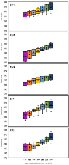
Figure 3.
Boxplots representing the variability of the DOY when each sugar level is reached (170 to 230 g L−1) at the selected sites (TN1, TN2, TN3, TF1 and TF2).
Regarding the climatic data used to develop the sugar ripeness models, the 2 m daily mean air temperatures were retrieved from the E-OBS dataset [37], supplied by the Copernicus Climate Change Service (C3S) platform. This widely used dataset provides observational gridded air-temperatures over a European-wide domain, at a relatively high spatial resolution (0.1° latitude × 0.1° longitude regular grid, ~10 km grid spacing) and includes data from, at least, one weather station located at the trial sites used for this work. Data for the five estates in the DS were extracted from the specific grid-box that covers each site. Ombrothermic diagrams for each year and each estate are shown as Supplementary Material (Figures S1–S5).
2.3. Model Parametrization and Calibration
Our approach attempts to model sugar concentration levels based on daily temperature observations. For this purpose, sigmoid models [21] were fitted to the existing sugar content data. Sigmoid models have been largely used to simulate grapevine phenology [13,22], and are considered some of the best modelling methodologies for this goal [19]. Model parametrization was carried out in the Phenological Modelling Platform (PMP, version 5.5), developed by INRAE (Paris, France) [38]. The PMP is a digital interface that aims to optimize, construct, and fit phenological models. It has been widely used in previous studies [13,16,25]. The Metropolis optimization algorithm [39] was herein used for the calibration and validation of temperature-based non-linear sigmoid models, presented in Equations (1) and (2):
where corresponds to the daily forcing rate, T to daily mean air temperature, the d-parameter to the sharpness of the sigmoid curve, and the e-parameter to the mid-curve temperature. The thermal forcing (Forc) necessary to reach the required sugar concentration level corresponds to the sum of the from flowering (t0) until the sugar concentration level DOY is reached.
The onset of the Forc accumulation was set at flowering in order to improve model accuracy, as the flowering date is an observational metric that can be easily obtained for real-time model calibration, and this date precedes sugar accumulation in berries, as they are not yet formed. Furthermore, the possibility to predict different sugar concentration dates at an early stage, such as flowering, is feasible and of foremost relevance for growers. This procedure was also undertaken by Rodrigues et al. (2021) in the Portuguese Dão wine region. In each of the five estates, flowering usually occurs in May, between DOY 120 and 150 (Figure 4). Flowering tends to occur later in TN1, mostly due to the higher elevation and consequently lower temperatures, while this stage occurs earlier in TF1 and TN2, owing to the higher temperatures during the growing season (Table 1). To better understand the prevailing conditions in the DS, the accumulated Forc between flowering (t0) and each level of sugar concentration until harvest were also estimated using PMP.
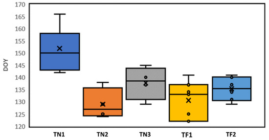
Figure 4.
The DOY of flowering, herein considered as t0 in the modelling approach (onset of the heat accumulation).
For the optimization of the developed models, different e- and d-parameters were tested to achieve the best fit, which provides the highest performance at each location and variety. As such, different e- and d-parameter values were thoroughly combined until a comprehensive and harmonized grapevine sugar ripeness model was found, which can subsequently be applied to the whole DS. Thus, three versions of the model were tested before reaching the final solution (Table S1). In the first version, the e- and d-parameters were computed by the PMP platform (free e and d in Table S1). This computation process is iterative, while the platform automatically selects the best performing parameters. Different values of e and d for each estate were then attained. Nonetheless, our goal is to deliver a model that is harmonized for the different estates in the DS and, ultimately, for the entire Douro. In version 2, the d-parameter was fixed, using the median value of all d-parameters in version 1 (d = −30). Lastly, in version 3, the e-parameter was also fixed, but dependent on location/estate. This approach was carried out to maximize the model efficiency, while still providing a regionally adapted model. A leave-one-out methodology was also performed to provide cross-validation (CV) of the model outputs. This methodology is often used whenever validation with an independent dataset is not possible due to small sample sizes. In our approach, we used both methodologies, i.e., CV and validation using an independent dataset. This is indeed a very common procedure, used in many different studies to assess model fitting performances [26].
2.4. Model Evaluation
Two evaluating metrics were used to assess the performance of the selected model, namely the root-mean-squared-error RMSE, Equation (3), the Nash–Sutcliffe coefficient efficiency EFF, and Equation (4), defined as follows:
where Xobs and Xpre are the observed and estimated values of each phenological phase, respectively, is the mean value of the observed dataset, and n is the number of observations used to optimize the model (sample size).
2.5. Model Validation
After model calibration, it is important to validate the models using different datasets. As was previously mentioned, the TF2 estate has a significantly longer temporal dataset of grape berry sugar concentration measurements, spanning from 1991–2020. Therefore, data from 1991–2013 (15 years) were also used to validate the sigmoid model results, thus allowing a more robust assessment of their performance.
2.6. Computer Application
Upon model development, a new computer application was developed (GSCM—Grapevine Sugar Concentration Model, Version 1.0, Vila Real, Portugal), which incorporates all the above-mentioned modelling procedures. This application was developed in MATLAB® App Designer version R2020b for the Windows operating system, although it could easily be converted/compiled into a web-application. The GSCM application uses the developed model and provides estimated dates for attaining the selected sugar concentrations. These projections are based on a time series of climatic data of the selected location, until the flowering date, combined with future temperature curves based on the climatology method [40]. This method is a simple technique for generating forecasts of specific sugar concentration timings based on statistics of the data gathered over multiple years (a 30-year period is usually recommended). Herein, we present three different statistics: the 25th, 50th, and 75th percentiles. Therefore, the application provides predictions depending on whether the target year will be within the median temperatures or cooler/warmer than average. The application is available within the CoaClimateRisk consortium for a testing period and will then be open-sourced for the general public.
3. Results
3.1. Model Training
A model sensitivity analysis was performed by exploring the d- and e-parameter values (Table S1). The d-parameter was eventually fixed at –30 (sharp direct sigmoid), whereas e was set independently at each location (TN1 = 18, TN2 = 21, TN3 = 19, TF1 = 19, and TF2 = 20). These values were selected based on the most skillful version of the sigmoid model (Table S1), aiming to achieve the highest EFF, while still reaching a model that can be easily adapted to different locations. The e-parameter corresponds to the mid-curve temperature in the sigmoid response function and is dependent on the grapevine variety (more or less heat demanding, or earlier or later ripening). However, it also tends to be related to the temperature at each location, suggesting some varietal adaptability to local conditions. These values are indeed strongly related to the annual mean temperatures of the five selected estates, showing a correlation coefficient of 0.69 (statistically significant at 99% confidence level). Our findings demonstrate that the optimized sigmoid models accomplished relatively high performance for all estates (Figure 5), showing that 69% (43%) of the models depict an EFF higher than 0.7 (0.8) (Table 2).
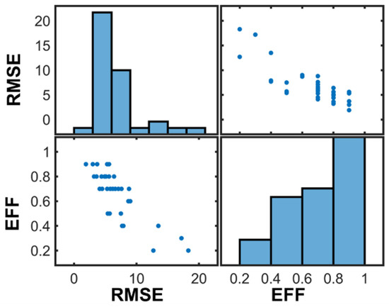
Figure 5.
Histograms and scatterplots showing the relationship between the RMSE and the EFF of the models developed for the five selected vineyard estates.
Table 2.
Metrics of the modelling of the sugar concentration (g L−1) for the five estates, including the RMSE and EFF (d- is fixed at −30 and t0 at the flowering date). All results shown are after leave-one-out cross-validation (CV).
Concerning the RMSE of the predictions (Figure 5), these were relatively low (<6 days on average), and lower than 4 days in 20% of the results. The highest errors (>10 days) were only found in 11% of the results. More specifically, an EFF of 0.9 was found for the sugar levels of 180, 210, and 230 g L−1, for TN1, TF2, and TF1, respectively, with an RMSE of 2–5 days. The lowest RMSE (<2 days) was found in TN2 for 210 g L−1 (Table 2). The highest RMSE was found in the first sugar levels (170 and 180 g L−1) for TN2 and TF2, surpassing 10 days, also showing the lowest EFF. At these two latter estates, the models performed worst in the first two sugar levels (170 and 180 g L−1), which may be attributed to the weaker relationship with the flowering date (t0). In effect, the model EFF increases significantly when simulating the following sugar levels (190, 200, 210, 220, and 230 g L−1). It is also worth noting that the two locations present higher e-parameter values, which may underlie these outcomes. Overall, the values of EFF and RMSE show a strong negative correlation (–0.83), thereby highlighting a high consistency between two performance metrics (Figure 5).
3.2. Thermal Accumulation and Sugar Relations
It is well known that grapevine responds directly to air, soil, and canopy temperatures [32]. The non-linear sigmoid function is directly connected to the critical sum of temperature units required to achieve a given sugar concentration level. Therefore, the sum of values (daily forcing rates) from t0 (accumulation onset) until the DOY of a given sugar level corresponds to the thermal accumulation threshold to reach that level (Forc). Figure 6 shows the Forc values, as a function of the sugar concentration and the e-parameter value. As expected, the Forc values tend to increase in response to higher sugar concentrations, inversely to the e-parameter value. Therefore, at locations with higher e values, such as the warmer TN2 and TF2, lower thermal accumulations are found, due to higher mid-curve temperature responses. Figure 6 also allows for the application and recreation of these models in additional locations, as long as an e-parameter value is defined.
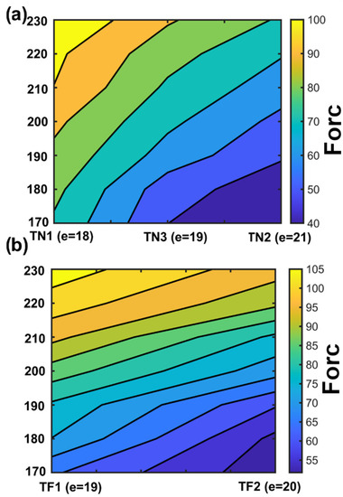
Figure 6.
Contour plots representing the grape berry sugar concentration level (primary y-axis) as a function of the Forc (secondary y-axis) and for each e-parameter value at each estate (x-axis).
3.3. Model Validation
Apart from using leave-one-out cross-validation, the model developed was also tested against an independent dataset, which was not used for calibration. Taking into account the chart in Figure 6 and the data in the validation period (1991–2013), the sigmoid model achieved an R2 = 0.93 (93% of represented variance by the model) and an RMSE < 5 days when compared to the observational and simulated sugar concentrations at the TF2 estate (Figure 7).
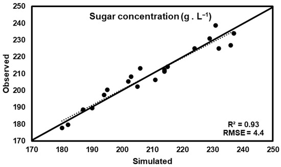
Figure 7.
Comparison between observed and simulated sugar concentration levels at harvest dates for the validation period (1991–2013) in the TF2 estate.
4. Computer Application
Given the high model efficiencies found, a standalone computer application was developed targeted at growers/farmers. This application (Figure 8), “GSCM—Grapevine Sugar Concentration Model” version 1.0, uses the following inputs: a climatic series of the chosen site (.csv file); the flowering date (t0); the e- and d-parameters; and the target sugar concentration to be modelled. As outputs, the application provides the estimated date in which the selected sugar concentration will be achieved, as well as a graphical display of the current year temperature (in comparison to the 25th, 50th, and 75th percentiles of all the mean temperatures found in the climate series file), as well as a graphical display of the estimated evolution of the sugar levels. The application also allows for the estimation of the best e-parameter (if the user does not know which is the e-parameter for his specific location). The e-parameter estimate is based on the previously mentioned relationship between the e-parameter values and the annual mean temperatures of each location, found in Figure 6.
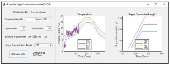
Figure 8.
Example of the computer application developed in the current study.
5. Discussion
Bearing in mind the principles of efficiency and parsimony in model development, our study seeks to find the best-fitted parameters, also avoiding overfitting problems. On this basis, after testing several models in PMP, new models were built. The performance metrics (EFF, RMSE) of the chosen model parametrizations indicate good performance using the same d- (–30) and changing e- for each site. The analysis of model sensitivity to changes in parameters (e and d) enabled the selection of the same sigmoid model, adapted at site-specific locations [27]. The calibration presented herein, based on efficiency and error metrics (performed under cross-validation), can be considered satisfactory, with an average EFF of 0.7 and an RMSE of 6 days (Table 2). The validation outputs show a very high performance in the TF2 site, reaching an R2 = 0.93 (Figure 7). Nonetheless, with the enlargement of the datasets from the CoaClimateRisk project partners, these can be improved in the future. In comparison, Parker et al. (2020), following a similar approach, modelled sugar ripeness reaching EFF > 0.5 and RMSE < 7 days. Our results hint at similar efficiency. Although the latter is one of the few available studies analyzing the development of a harvest date model based on sugar concentrations, the sigmoid models have been demonstrating a good response in phenology simulation. For instance, Reis et al. (2020) used different d- and e- parameters for modelling phenology in four Portuguese wine regions using sigmoid models. Moreover, for the Dão wine region [27], these models (EFF > 0.81, RMSE < 6 days) were used to simulate sugar concentration and acidity at harvest.
Other aspects related to the specific site conditions of the DS region should also be considered, which may enhance the robustness of the developed models. During the calibration period (2014–2020), harvest dates in the DS took place between 15 August (DOY 227) and the end of October (DOY 304), considering TN and TF cultivars and the five locations (Figure 2). This is quite a large interval in comparison to other winemaking regions in Europe, thus supporting the temporal variability in our results and their validity. Hence, the developed model can be accurately applied in the warm and dry conditions of the DS, by duly taking into account the commonly large interannual variability. As such, this new model, based on daily air temperature, can be easily implemented by local growers, with minimal fine-tuned changes depending on the location.
The characteristics of the grape berries directly influence the quality of the wine and the harvest schedule. Information about sugar accumulation, combined with compound concentrations, such as anthocyanins and polyphenols, total acidity, and pH, may determine the adequate harvest time for each growing cycle and year. Nonetheless, the harvest date is extremely difficult to accurately model and simulate, particularly in the DS. As an example, Van Leeuwen et al. (2019) [41] state that, in the Bordeaux wine region, white grapes are picked around a grape sugar level of 210 g L−1 (12.5 % potential alcohol), while red cultivars tend to be harvested approximately 15 days later, as they are generally picked at a sugar level of roughly 230 g L−1 (13.5 % potential alcohol). This is not exactly the case of the DS, where terrain characteristics and elevation may also play major roles, besides air temperature variability. Furthermore, in the DS, port fortified wines and Douro table wines tend to follow different pathways regarding the choice of the maturation as a function of grape berry quality parameters, which is another aspect to consider.
Harvesting is ultimately a grower’s decision, making the mechanistic forecast challenging. According to Figure 3, harvest in the DS is usually carried out at different levels of sugar concentrations (usually from 190 to 230 g L−1), showing that from harvest decision to harvest operation there is indeed an influence by factors other than maturity. In the past, the use of sugar concentration as a measure of “ripeness” was not usually considered for the classification of grapevine varieties regarding their thermal requirements. The present study approach follows the work laid out by Parker et al. (2020), using Portuguese cultivars under warm climate viticulture. The model developed may provide growers with an optimum timeframe for sugar concentrations, which, in turn, may provide forecasts of technical maturity and harvest timings. These simulations will be of key importance for growers since the harvest date is one of the most important events for the proper planning of the annual vineyard activities and in defining the initial quality potential of wines to be produced. Several important resources must be scheduled for planning this major event in the vineyards, such as human resources, proper machinery tuning, distribution, management, and financial aspects.
Some limitations of the current modelling approach should also be outlined. The difficulty in comparing cultivars at different locations is amongst the most relevant, on top of not controlling the clonal diversity existing in plantations of such varieties. Another aspect is related to the wine type, e.g., the Douro table wines versus port fortified wines. It should also be stated that maturation is not exclusively dependent on sugar concentration. Other factors, such as pH and total acidity, may also play a key role. Other atmospheric-driven variables besides air/plant temperature, such as soil water content, air humidity, radiation fluxes, wind, extreme weather events (e.g., hail, wind gusts, heavy precipitation, heat waves, late frost), as well as canopy microclimates, may also contribute to the grapevine phenology and grape berry maturation. Furthermore, management issues, such as human/labour resources or machinery, frequently influence harvest timings, though these driving factors are out of the scope of the present study.
The DS winemaking region is located in a “climate change hotspot”, meaning that the impacts of climate change in this region may be particularly severe [42]. Current studies indicate that this particular sub-region of the Douro PDO may be negatively affected in terms of viticultural productivity [43], particularly due to the increase in extreme weather events [42,44]. In effect, climate change impacts on viticulture are already being reported in different regions worldwide, such as the shift in phenology, higher sugar concentration, and late spring frost problems [45,46,47,48,49]. Although the grapevine is a very resilient species to adverse climatic conditions, future climates may threaten the winemaking economic revenue in this region [43]. Grapevine phenology is being increasingly modified by higher temperatures in DS, enhancing the need for adaptation strategies, in both the short [17] and long term [18]. Adaptation measures that allow better planning of harvest dates, avoiding the hottest and driest period of the year (summer maximum, August), and, in some cases, also avoiding periods with excessive precipitation, are particularly pertinent.
6. Conclusions
Grapevine sugar concentration models were developed in this study and may be used for forecasting harvest dates in the Douro Superior winemaking sub-region. By developing a methodology that can be easily adapted for any specific location, it was possible to calibrate the models with an efficiency of more than 0.7, and an error lower than 6 days. A model validation, using 15 years of independent data, showed a very high correlation with observational data. A computer application was then developed, allowing a practical use of the developed models by growers and stakeholders. These modelling tools can not only be easily adopted by the DS growers to better plan their viticultural and winemaking activities, but can also be used as a decision-support instrument to adapt against the detrimental impacts of climate change, reducing risks and enhancing long-term sustainability.
Supplementary Materials
The following supporting information can be downloaded at: https://www.mdpi.com/article/10.3390/agronomy12061404/s1, Figure S1: Bagnols & Gaussen diagram for each year separately and for estate TN1. Yellow curves correspond to the daily mean temperature (in °C, left y-axis), while blue bars correspond to the daily total precipitation (in mm, right y-axis). Figure S2: As in Figure S1 but estate TN2. Figure S3: As in Figure S1 but estate TN3. Figure S4: As in Figure S1 but estate TF1. Figure S5: As in Figure S1 but estate TF2. Table S1: Three versions of the models used in the present study. All models are performed under cross-validation for each location.
Author Contributions
Conceptualization, H.F.; methodology, H.F. and N.C.; software, H.F.; validation, H.F., N.C. and J.A.S.; formal analysis, N.C.; investigation, N.C. and H.F.; resources, H.F.; data curation, N.C., N.F., A.G. and I.G.; writing—original draft preparation, H.F. and N.C.; writing—review and editing, N.C., J.A.S., N.F., A.G., I.G. and H.F.; visualization, H.F.; supervision, H.F.; project administration, H.F.; funding acquisition, H.F. All authors have read and agreed to the published version of the manuscript.
Funding
The work was funded by the CoaClimateRisk project (COA/CAC/0030/2019) financed by National Funds by the Portuguese Foundation for Science and Technology (FCT).
Data Availability Statement
Not applicable.
Acknowledgments
The work was funded by the CoaClimateRisk project (COA/CAC/0030/2019) financed by National Funds by the Portuguese Foundation for Science and Technology (FCT). This work was also supported by National Funds by FCT, under the projects UIDB/04033/2020 and LA/P/0126/2020. Helder Fraga thanks the FCT for the contract CEECIND/00447/2017. We acknowledge the E-OBS dataset from the EU-FP6 project UERRA (https://www.uerra.eu) and the Copernicus Climate Change Service, and the data providers in the ECA&D project (https://www.ecad.eu (accessed on 29 January 2022)). We thank Sogrape and ADVID for providing the grapevine phenological and grape quality parameter data sets used in this study. The GSCM application was developed by Helder Fraga.
Conflicts of Interest
The authors declare no conflict of interest.
References
- Droulia, F.; Charalampopoulos, I. Future Climate Change Impacts on European Viticulture: A Review on Recent Scientific Advances. Atmosphere 2021, 12, 495. [Google Scholar] [CrossRef]
- Wolkovich, E.M.; Burge, D.O.; Walker, M.A.; Nicholas, K.A. Phenological Diversity Provides Opportunities for Climate Change Adaptation in Winegrapes. J. Ecol. 2017, 105, 905–912. [Google Scholar] [CrossRef] [Green Version]
- Moriondo, M.; Jones, G.V.; Bois, B.; Dibari, C.; Ferrise, R.; Trombi, G.; Bindi, M. Projected Shifts of Wine Regions in Response to Climate Change. Clim. Change 2013, 119, 825–839. [Google Scholar] [CrossRef]
- Molitor, D.; Junk, J. Climate Change Is Implicating a Two-Fold Impact on Air Temperature Increase in the Ripening Period under the Conditions of the Luxembourgish Grapegrowing Region. Oeno One 2019, 53, 409–422. [Google Scholar] [CrossRef]
- Verdenal, T.; Zufferey, V.; Dienes-Nagy, A.; Bourdin, G.; Gindro, K.; Viret, O.; Spring, J.-L. Timing and Intensity of Grapevine Defoliation: An Extensive Overview on Five Cultivars in Switzerland. Am. J. Enol. Vitic. 2019, 70, 427–434. [Google Scholar] [CrossRef]
- Fraga, H.; Santos, J.A.; Malheiro, A.C.; Oliveira, A.A.; Moutinho-Pereira, J.; Jones, G.V. Climatic Suitability of Portuguese Grapevine Varieties and Climate Change Adaptation. Int. J. Climatol. 2016, 36, 1–12. [Google Scholar] [CrossRef]
- Cataldo, E.; Salvi, L.; Paoli, F.; Fucile, M.; Mattii, G.B. Effects of Defoliation at Fruit Set on Vine Physiology and Berry Composition in Cabernet Sauvignon Grapevines. Plants 2021, 10, 1183. [Google Scholar] [CrossRef]
- IPCC; Stocker, T.F.; Qin, D.; Plattner, G.-K.; Tignor, M.; Allen, S.K.; Boschung, J.; Nauels, A.; Xia, Y.; Bex, V.; et al. Climate Change 2013: The Physical Science Basis. In Contribution of Working Group I to the Fifth Assessment Report of the Intergovernmental Panel on Climate Change; Cambridge University Press: Cambridge, UK; New York, NY, USA, 2013. [Google Scholar]
- Fraga, H.; Santos, J.A. Assessment of Climate Change Impacts on Chilling and Forcing for the Main Fresh Fruit Regions in Portugal. Front. Plant Sci. 2021, 12, 689121. [Google Scholar] [CrossRef]
- Jones, G.V.; Davis, R.E. Climate Influences on Grapevine Phenology, Grape Composition, and Wine Production and Quality for Bordeaux, France. Am. J. Enol. Vitic. 2000, 51, 249–261. [Google Scholar]
- de Rességuier, L.; Mary, S.; Le Roux, R.; Petitjean, T.; Quénol, H.; van Leeuwen, C. Temperature Variability at Local Scale in the Bordeaux Area. Relations With Environmental Factors and Impact on Vine Phenology. Front. Plant Sci. 2020, 11, 515. [Google Scholar] [CrossRef]
- Orlandi, F.; Bonofiglio, T.; Aguilera, F.; Fornaciari, M. Phenological Characteristics of Different Winegrape Cultivars in Central Italy. VITIS—J. Grapevine Res. 2015, 54, 129–136. [Google Scholar] [CrossRef]
- Reis, S.; Fraga, H.; Carlos, C.; Silvestre, J.; Eiras-Dias, J.; Rodrigues, P.; Santos, J.A. Grapevine Phenology in Four Portuguese Wine Regions: Modeling and Predictions. Appl. Sci. 2020, 10, 3708. [Google Scholar] [CrossRef]
- Cataldo, E.; Fucile, M.; Mattii, G.B. Effects of Kaolin and Shading Net on the Ecophysiology and Berry Composition of Sauvignon Blanc Grapevines. Agriculture 2022, 12, 491. [Google Scholar] [CrossRef]
- Leng, F.; Wang, C.; Sun, L.; Li, P.; Cao, J.; Wang, Y.; Zhang, C.; Sun, C. Effects of Different Treatments on Physicochemical Characteristics of ‘Kyoho’ Grapes during Storage at Low Temperature. Horticulturae 2022, 8, 94. [Google Scholar] [CrossRef]
- Caffarra, A.; Eccel, E. Increasing the Robustness of Phenological Models for Vitis Vinifera Cv. Chardonnay. Int. J. Biometeorol. 2010, 54, 255–267. [Google Scholar] [CrossRef]
- Santos, J.A.; Yang, C.; Fraga, H.; Malheiro, A.C.; Moutinho-Pereira, J.; Dinis, L.-T.; Correia, C.; Moriondo, M.; Bindi, M.; Leolini, L.; et al. Short-Term Adaptation of European Viticulture to Climate Change: An Overview from the H2020 Clim4Vitis Action. IVES Tech. Rev. Vine Wine 2021. [Google Scholar] [CrossRef]
- Santos, J.A.; Yang, C.; Fraga, H.; Malheiro, A.C.; Moutinho-Pereira, J.; Dinis, L.-T.; Correia, C.; Moriondo, M.; Bindi, M.; Leolini, L.; et al. Long-Term Adaptation of European Viticulture to Climate Change: An Overview from the H2020 Clim4Vitis Action. IVES Tech. Rev. Vine Wine 2021. [Google Scholar] [CrossRef]
- Costa, R.; Fraga, H.; Fonseca, A.; De Cortázar-Atauri, I.G.; Val, M.C.; Carlos, C.; Reis, S.; Santos, J.A. Grapevine Phenology of Cv. Touriga Franca and Touriga Nacional in the Douro Wine Region: Modelling and Climate Change Projections. Agronomy 2019, 9, 210. [Google Scholar] [CrossRef] [Green Version]
- de Reaumur, R.A.F. Observations Du Thermomètre, Faites à Paris Pendant l’année 1735, Comparées Avec Celles Qui Ont Été Faites Sous La Ligne, à l’isle de France, à Alger et Quelques Unes de Nos Isles de l’Amérique. Mem. Paris Acad. Sci. 1735, 545. [Google Scholar]
- Hanninen, H. Modelling Bud Dormancy Release in Trees from Cool and Temperate Regions. Acta For. Fenn. 1990, 213. [Google Scholar] [CrossRef] [Green Version]
- Parker, A.K.; García de Cortázar-Atauri, I.; Gény, L.; Spring, J.L.; Destrac, A.; Schultz, H.; Molitor, D.; Lacombe, T.; Graça, A.; Monamy, C.; et al. Temperature-Based Grapevine Sugar Ripeness Modelling for a Wide Range of Vitis vinifera L. Cultivars. Agric. For. Meteorol. 2020, 285–286, 107902. [Google Scholar] [CrossRef]
- de Cortázar-Atauri, I.G.; Brisson, N.; Gaudillere, J.P. Performance of Several Models for Predicting Budburst Date of Grapevine (Vitis vinifera L.). Int. J. Biometeorol. 2009, 53, 317–326. [Google Scholar] [CrossRef] [PubMed]
- Parker, A.K.; De Cortázar-Atauri, I.G.; Van Leeuwen, C.; Chuine, I. General Phenological Model to Characterise the Timing of Flowering and Veraison of Vitis vinifera L. Aust. J. Grape Wine Res. 2011, 17, 206–216. [Google Scholar] [CrossRef]
- Leolini, L.; Costafreda-Aumedes, S.; Santos, J.A.; Menz, C.; Fraga, H.; Molitor, D.; Merante, P.; Junk, J.; Kartschall, T.; Destrac-Irvine, A.; et al. Phenological Model Intercomparison for Estimating Grapevine Budbreak Date (Vitis vinifera L.) in Europe. Appl. Sci. 2020, 10, 3800. [Google Scholar] [CrossRef]
- Piña-rey, A.; Ribeiro, H.; Fernández-gonzález, M.; Abreu, I.; Javier Rodríguez-Rajo, F. Phenological Model to Predict Budbreak and Flowering Dates of Four Vitis Vinifera L. Cultivars Cultivated in DO. Ribeiro (North-West Spain). Plants 2021, 10, 502. [Google Scholar] [CrossRef]
- Rodrigues, P.; Pedroso, V.; Gonçalves, F.; Reis, S.; Santos, J.A. Temperature-Based Grapevine Ripeness Modeling for Cv. Touriga Nacional and Encruzado in the Dão Wine Region, Portugal. Agronomy 2021, 11, 1777. [Google Scholar] [CrossRef]
- Suter, B.; Destrac Irvine, A.; Gowdy, M.; Dai, Z.; van Leeuwen, C. Adapting Wine Grape Ripening to Global Change Requires a Multi-Trait Approach. Front. Plant Sci. 2021, 12, 36. [Google Scholar] [CrossRef]
- de Figueiredo, T.; Martins, A.; Hernández, Z.; Carlos, C.; Fonseca, F. Proteção Do Solo Em Viticultura de Montanha: Manual Técnico Para a Região Do Douro. In Proteção do Solo em Viticultura de Montanha Manual Técnico para a Região do Douro; ADVID—Associação para o Desenvolvimento da Viticultura Duriense: Vila Real, Portugal, 2015; Volume 25. [Google Scholar]
- Food and Agriculture Organization of the United Nations. World Reference Base for Soil Resources 2014: International Soil Classification System for Naming Soils and Creating Legends for Soil Maps; FAO: Rome, Italy, 2014. [Google Scholar]
- Fraga, H.; de Atauri, I.G.C.; Malheiro, A.C.; Moutinho-Pereira, J.; Santos, J.A. Viticulture in Portugal: A Review of Recent Trends and Climate Change Projections. OENO One 2017, 51, 61–69. [Google Scholar] [CrossRef] [Green Version]
- Van Leeuwen, C.; Roby, J.P.; De Rességuier, L. Soil-Related Terroir Factors: A Review. OENO One 2018, 52, 173–188. [Google Scholar] [CrossRef] [Green Version]
- Bagnouls, F.; Gaussen, H. Les Climats Biologiques et Leur Classification. Ann. Géographie 1957, 66, 193–220. [Google Scholar] [CrossRef]
- Lorenz, D.H.; Eichorn, K.W.; Bleiholder, H.; Klose, R.; Meier, U.; Weber, E. Growth Stages of the Grapevine: Phenological Growth Stages of the Grapevine (Vitis vinifera L. Ssp. Vinifera)—Codes and Descriptions According to the Extended BBCH Scale†. Aust. J. Grape Wine Res. 1995, 1, 100–103. [Google Scholar] [CrossRef]
- Costa, C.; Graça, A.; Fontes, N.; Teixeira, M.; Gerós, H.; Santos, J.A. The Interplay between Atmospheric Conditions and Grape Berry Quality Parameters in Portugal. Appl. Sci. 2020, 10, 4943. [Google Scholar] [CrossRef]
- OIV, I.O.O.V.A.W. OIV—Compendium of International Methods of Analysis of Wines and Musts; OIV: Paris, France, 2012. [Google Scholar]
- Cornes, R.C.; van der Schrier, G.; van den Besselaar, E.J.M.; Jones, P.D. An Ensemble Version of the E-OBS Temperature and Precipitation Data Sets. J. Geophys. Res. Atmos. 2018, 123, 9391–9409. [Google Scholar] [CrossRef] [Green Version]
- Chuine, I.; De Cortazar-Atauri, I.G.; Kramer, K.; Hänninen, H. Plant Development Models. Phenol. Integr. Environ. Sci. 2013, 275–293. [Google Scholar] [CrossRef]
- Metropolis, N.; Rosenbluth, A.W.; Rosenbluth, M.N.; Teller, A.H.; Teller, E. Equation of State Calculations by Fast Computing Machines. J. Chem. Phys. 1953, 21, 1087–1093. [Google Scholar] [CrossRef] [Green Version]
- van den Dool, H. Empirical Methods in Short-Term Climate Prediction; OUP Oxford: Oxford, UK, 2007; ISBN 9780199202782. [Google Scholar]
- Van Leeuwen, C.; Destrac-Irvine, A.; Dubernet, M.; Duchêne, E.; Gowdy, M.; Marguerit, E.; Pieri, P.; Parker, A.; De Rességuier, L.; Ollat, N. An Update on the Impact of Climate Change in Viticulture and Potential Adaptations. Agronomy 2019, 9, 514. [Google Scholar] [CrossRef] [Green Version]
- Fraga, H.; Molitor, D.; Leolini, L.; Santos, J.A. What Is the Impact of Heatwaves on European Viticulture? A Modelling Assessment. Appl. Sci. 2020, 10, 3030. [Google Scholar] [CrossRef]
- Fraga, H.; Guimarães, N.; Freitas, T.R.; Malheiro, A.C.; Santos, J.A. Future Scenarios for Olive Tree and Grapevine Potential Yields in the World Heritage Côa Region, Portugal. Agronomy 2022, 12, 350. [Google Scholar] [CrossRef]
- Martins, J.; Fraga, H.; Fonseca, A.; Santos, J.A. Climate Projections for Precipitation and Temperature Indicators in the Douro Wine Region: The Importance of Bias Correction. Agronomy 2021, 11, 990. [Google Scholar] [CrossRef]
- Duchene, E.; Huard, F.; Dumas, V.; Schneider, C.; Merdinoglu, D. The Challenge of Adapting Grapevine Varieties to Climate Change. Clim. Res. 2010, 41, 193–204. [Google Scholar] [CrossRef] [Green Version]
- White, M.A.; Diffenbaugh, N.S.; Jones, G.V.; Pal, J.S.; Giorgi, F. Extreme Heat Reduces and Shifts United States Premium Wine Production in the 21st Century. Proc. Natl. Acad. Sci. USA 2006, 103, 11217–11222. [Google Scholar] [CrossRef] [PubMed] [Green Version]
- van Leeuwen, C.; Darriet, P. The Impact of Climate Change on Viticulture and Wine Quality. J. Wine Econ. 2016, 11, 150–167. [Google Scholar] [CrossRef] [Green Version]
- Hannah, L.; Roehrdanz, P.R.; Ikegami, M.; Shepard, A.V.; Shaw, M.R.; Tabor, G.; Zhi, L.; Marquet, P.A.; Hijmans, R.J. Climate Change, Wine, and Conservation. Proc. Natl. Acad. Sci. USA 2013, 110, 6907–6912. [Google Scholar] [CrossRef] [PubMed] [Green Version]
- Jones, G.V.; White, M.A.; Cooper, O.R.; Storchmann, K. Climate Change and Global Wine Quality. Clim. Change 2005, 73, 319–343. [Google Scholar] [CrossRef]
Publisher’s Note: MDPI stays neutral with regard to jurisdictional claims in published maps and institutional affiliations. |
© 2022 by the authors. Licensee MDPI, Basel, Switzerland. This article is an open access article distributed under the terms and conditions of the Creative Commons Attribution (CC BY) license (https://creativecommons.org/licenses/by/4.0/).