Abstract
The sowing date and density are considered to be the main factors affecting crop yield. The determination of the sowing date and sowing density, however, is fraught with uncertainty due to the influence of climatic conditions, topography, variety and other factors. Therefore, it is necessary to find a comprehensive consideration of these factors to guide the production of winter rapeseed. A reliable crop model could be a crucial tool to investigate the response of rapeseed growth to changes in the sowing date and density. At present, few studies related to rapeseed model simulation have been reported, especially in the comprehensive evaluation of the effects of sowing date and density factors on rapeseed development and production. This study aimed to evaluate the performance of the AquaCrop model for winter rapeseed development and yield simulation under various sowing dates and densities, and to optimize the sowing date and density for agricultural high-efficient production in the Jianghuai Plain. Two years of experiments were carried out in the rapeseed growing season in 2020 and 2021. The model parameters were fully calibrated and the simulation performances in different treatments of sowing dates and densities were evaluated. The results indicated that the capability of the AquaCrop model to interpret crop development for different sowing dates was superior to that of sowing densities. For rapeseed canopy development, the RMSE for three sowing dates and densities scenarios were 7–22% and 16–23%, respectively. The simulated biomass and grain yield for different sowing dates treatments (RMSE: 0.8–2.1 t·ha−1, Pe: 0–35.3%) were generally better than those of different densities treatments (RMSE: 0.7–3.9 t·ha−1, Pe: 8.2–90%). Compared with other sowing densities, higher overestimation errors of the biomass and yield were observed for the low-density treatment. Adequate agreement for crop evapotranspiration simulation was achieved, with an R2 of 0.79 and RMSE of 26 mm. Combining the simulation results and field data, the optimal sowing scheme for achieving a steadily high yield in the Jianghuai Plain of east China was determined to be sowing in October and a sowing density of 25.0–37.5 plant·m−2. The study demonstrates the great potential of the AquaCrop model to optimize rapeseed sowing patterns and provides a technical means guidance for the formulation of local winter rapeseed production.
1. Introduction
Rapeseed (Brassica napus L.), the third-largest oilseed crop in the world, is used to produce edible oil, feed protein and biodiesel [1]. As one of the main planting countries, China accounts for 15.6% of the global rapeseed total sown area and 17.4% of the total yield: FAOSTAT, https://www.fao.org/faostat/en. (accessed on 1 June 2022). In 2020, the rapeseed sown area and yield made up 51.5% and 39.2% of oil crops in China, respectively [2]. As the primary oilseed crop grown in the Jianghuai Plain, the winter rapeseed is typically planted in rotation with rice to enhance the efficiency of land use. Due to the complexity of climate change, rapeseed sowing dates are constantly adjusted [3]. Therefore, it is crucial to clarify the response of rapeseed growth to the change in sowing dates for guiding field management practices and improving rapeseed production.
Previous studies revealed that the variations of the sowing date directly determined the rapeseed growth and development. Delayed sowing dates usually shortened the growth period and lowered the harvest index (HI). Moreover, a later sowing date could decrease the branch number and pod number, resulting in yield reduction [4,5]. Kirkegaard et al. [6] found that with the delay of the sowing date, the stress caused by low temperatures and other factors reduced the yield of rapeseed and the oil content. In addition, the sowing density is another significant factor dominating the rapeseed yield. A higher sowing density increases crop canopy coverage and canopy light utilization, and reduces soil evaporation, hence resulting in a high yield [7]. The study demonstrated that although the per plant number of branches and pods would be decreased with an increasing sowing density, the number of effective pods increased at the population level, which led to an improvement in rapeseed production at high densities [8]. However, crop yields begin to decline over a certain sowing density, due to intense competition between plants and limited light, nutrients and water conditions [9,10].
To date, some studies have been conducted on the response of rapeseed development to the sowing date and density in different regions and climatic conditions [11,12,13]. For example, Guan et al. [14] investigated the variation of rapeseed yields under different sowing dates and densities in Hunan Province, south of China, which revealed that appropriate late sowing and increased sowing density can reduce the seasonal contradiction between double-cropping rice and rapeseed sowing while ensuring a stable rapeseed yield. Wu et al. [6]. studied the effects of the sowing date and density on yields for direct-sown rapeseed, and indicated that the sowing date was the main factor affecting the plant height, primary branch number and yield of rapeseed, and early sowing was beneficial to obtain a high yield. When the sowing date is delayed, increasing the sowing density can compensate for the effect of late sowing on the yield. Li et al. [15] explored the effects of different sowing dates and density conditions on rapeseed field agronomic traits. The results indicated that with the postponement of the sowing date, the field weed coverage and lodging were increased, which suppressed rapeseed growth and damaged the rapeseed yield, while the yield could be compensated by increasing the sowing density to inhibit weeds to reduce lodging and increase the yield. However, most previous studies focused on short-term field experiments, and the results were highly uncertain due to the changing of crop varieties, soil conditions and climate types, especially in the frequent occurrence of extreme climates over recent years.
A crop growth model is an effective tool to quantify the impacts of the environment, climate and field management measures on crop growth. It can completely simulate the process of crop development, and incorporate the influence of external factors that have been widely used in agricultural prediction, climate change impact assessments, agricultural decision making and optimized cultivation mode [16,17,18,19,20]. In recent studies, most well-known models have been calibrated and validated to simulate the development and grain yield of rapeseed under different scenarios. For example, Mousavi et al. [21] used the SWAP model to model the development of rapeseed by two cultivation periods in Badjgah and the rapeseed yield simulation results showed that the normalized root mean square error (nRMSE) was 8.0% and 14.2%, respectively. Jing et al. [22] used the DSSAT -CROPGRO model to simulate spring rapeseed growth under different nitrogen application rates in eastern Canada and the results showed that satisfactory accuracy was achieved for the aboveground biomass simulation, with an nRMSE of 19%. He et al. [23] evaluated the capability of the APSIM–Canola model to simulate rapeseed phenology and the impact of phenology on the simulated yield (RMSE for days of flowering and maturity: 1.9–4.2 days). Qian et al. [24] simulated crop yields using the DSSAT-CERES-Wheat and DSSAT–CROPGRO–Canola models driven by estimated and measured daily solar radiation data. The results indicated that the deviations of the two sets of data for wheat and rapeseed yield estimation were 5% and 12%, respectively. However, most of the studies investigated the response of rapeseed to different environmental changes under a single sowing pattern [25,26,27,28]. Limited studies have been conducted on simulating rapeseed growth and development; especially, a performance evaluation of the model for the growth of rapeseed with different sowing dates and densities has not been reported.
Therefore, to explore the optimal sowing date and density for producing high rapeseed biomass and yields, two seasons of rapeseed field experiments in 2020 and 2021 were conducted with the consideration of different sowing dates and densities scenarios. The AquaCrop model, a famous water-driven crop simulation model, was employed to simulate winter rapeseed development and yield [29]. Compared with other models, the AquaCrop model only requires explicit and intuitive input parameters and has a good user interface. However, the model has less research on crop growth simulation in rain-fed areas, and there are also large differences in the selection of conservative parameters and non-conservative parameters [30]. The objectives of this study were to: (1) reveal the response of rapeseed growth under various sowing dates and densities conditions; (2) evaluate the capability of the model for interpreting the variation of canopy coverage, biomass, yield and evapotranspiration of winter rapeseed; and (3) determine the optimal sowing date and density of winter rapeseed in the Jianghuai Plain.
2. Materials and Methods
2.1. Study Area
The data used in this study were obtained from the filed experiments conducted at an ecological experimental station (Figure 1). It is located in the Jianghuai Plain of eastern China (32°21′ N, 119°24′ E, 5 m above sea level). The research site is located in a subtropical monsoon climate, with an annual precipitation and average temperature of 1063 mm and 14.8 °C, respectively. The predominant soil at the site is classified as the loamy, with an average field capacity of 0.35 cm3·cm−3, permanent wilting point of 0.13 cm3·cm−3 and dry bulk density of 1.49 g·cm−3. The soil initial nutrient contents in the 0–20 cm surface layer were as follows: mass fraction of organic matter 10.2 g·kg−1, total nitrogen 0.97 g·kg−1, available phosphorus 16.3 mg·kg−1 and available potassium 151.2 mg·kg−1, respectively [31].
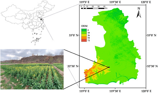
Figure 1.
The location map of the study area and test field photos, black marker point represents the location of the test station.
2.2. Experimental Design
A split-plot experiment was performed and conducted in two growing seasons, with the sowing date as the main plot, and sowing density as the subplot (Table 1). Referring to the local common sowing time, four sowing time periods were set as: early (ES), normal (NS1 and NS2) and late (LS) sowing. In addition, three sowing densities of low density (LD), medium density (MD) and high density (HD) were set for each of the sowing dates. Each sowing treatment had three replicates. The plot size was 5 m × 5 m, with a row spacing of 0.4 m. The seedlings were thinned manually by the 5-leaf stage to achieve the designed density. All treatments were carried out under rainfed conditions, and other field management practices (e.g., weeding, insecticidal and disease prevention) were consistent with local practices. The winter rapeseed was harvested in the May of next year.

Table 1.
Different sowing dates and density treatments in 2020 and 2021 growing seasons.
2.3. Field Data Collection
2.3.1. Canopy Cover
The AquaCrop model uses the canopy coverage (CC) instead of the leaf area index (LAI) to express crop development. CC is usually defined as the percentage of the vertical projected area of crop (including stems and leaves) within the unit area [32]. In this study, the data of the winter rapeseed CC were extracted by the vegetation index threshold method proposed by Jiapaer and Niu et al. [33,34]. Images, for winter rapeseed CC extraction, were collected by a multispectral camera (Rededge-MX, MicaSense Inc., Seattle, WA, USA) mounted on DJI Inspire 2 (DJI Inc., Shenzhen, Guangdong, China). After image processing, the CC of different plots was extracted and calculated using Equation (1). The normalized difference vegetation index (NDVI) images were extracted and verified for bare soil, seedlings and the maximum canopy of the winter rapeseed images (Figure 2), and the NDVI value of 0.46 was determined as the threshold for the extraction of CC, thus the pixels of the NDVI below the threshold were represented as soil backgrounds. Canopy coverage is extracted at approximately 20–30 days.
where is the number of winter rapeseed pixels and is the number of soil background pixels.
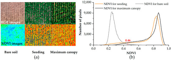
Figure 2.
Extracting CC schematic by using threshold method. (a) Winter rapeseed RGB images and NDVI images extracted based on threshold method at different growth stages. (b) Soil and winter rapeseed histogram distribution statistics based on NDVI.
2.3.2. Aboveground Dry Biomass and Yield
The aboveground dry biomass (AGB) was measured 3–6 times per growing season. In order to avoid the boundary effect, 10 samples were randomly collected from the center of each plot. The samples were weighed and then dried in an oven at 75 °C for three days until they reached a steady weight. The dry weight of the sample was measured, and the dry matter mass per unit area was calculated by multiplying the dry matter mass per plant by the sowing density. The pods were collected when two-thirds of the pods in the plot were brown. Ten plants per plot were randomly sampled and harvested until crop maturity. Then, the seed yield per plant was measured.
2.3.3. Crop Evapotranspiration
The crop evapotranspiration (ETC) for winter rapeseed is calculated by the water balance method (Equation (2)) [35].
where is evapotranspiration (mm), is the soil water content before sowing (mm), is the soil water content in the harvest period (mm), is the effective precipitation during the whole growth period (mm), is the irrigation amount during the whole growth period (mm), is surface runoff (mm), is deep drainage (mm) and the precipitation exceeding field capacity is regarded as and .
The experiment was carried out under rainfed conditions; hence, the IW was zero. A 50 cm layer was calculated in this study with an average field capacity of 0.35 cm3 cm−3, so when rainfall is greater than 175 mm, the excess is regarded as R and Sd.
2.4. Model Description
AquaCrop, a water-driven model, was evolved from the water production function proposed by Doorenbos et al. [36]. The model separated the actual crop evapotranspiration (ET) into crop transpiration (Tr) and soil evaporation (E), and calculated the yield by the aboveground dry biomass using the harvest index [29]. The main processes of the crop simulation can be described as the following steps:
- (1)
- The crop development process: AquaCrop employs the CC to describe the development of crops. Three parameters of the initial canopy coverage, maximum canopy coverage and canopy growth coefficient were used to determine the dynamic of the crop canopy coverage.
- (2)
- Crop evapotranspiration: ET simulation is divided into Tr and E. Based on the given meteorological data, the reference evapotranspiration (ET0) is calculated by the Penmane–Monteith equation in the FAO Irrigation and Drainage Paper No. 566 [35]. Tr is calculated by the product of ET0 and the crop transpiration coefficient (KcTr), and the KcTr is proportional with the CC. Soil evaporation is calculated by multiplying ET0 with the soil evaporation coefficient, a coefficient that relates to the fraction of uncovered soil surface.
- (3)
- Biomass: The output of the model simulation biomass was the AGB, excluding root and tuber crops. The model uses normalized water productivity (WP*) and Tr for estimating the biomass (Equation (3)). The WP* indicates the produced dry matter (g) per unit land area (m2) per unit of transpired water amount (mm). The WP* can be supposed to be the constant of the given crops and growth conditions (e.g., C3 crops: 15–20 g·m−2, C4 crops: 30–35 g·m−2) suggested by Steduto et al. [37].
- (4)
- Crop yield: After determining the crop biomass, the yield formation is obtained by the product of biomass and HI (Equation (4)).
2.5. Input Data and Model Calibration
The input data of the AquaCrop model are divided into four categories: meteorological data, crop data, management data and soil data. These input parameters can be divided into conservative and non-conservative parameters during model calibration. Conservative parameters are assumed to be unchanged with time, management practice or location, and can be used as the default values for model input. They include, for example, the crop maximum transpiration coefficient, water productivity, reference harvest index and water stress threshold for inhibiting leaf growth, stomatal conductance and accelerating canopy senescence. Non-conservative parameters, also known as user variety-specific parameters, include weather, soil, crop phenology and field management data in addition to crop parameters (e.g., sowing density and date) [10]. The input data and detailed model calibration are described in Section 2.5.1, Section 2.5.2 and Section 2.5.3.
2.5.1. Weather Data
The basic input meteorological data imputing into the AquaCrop model include temperature (maximum and minimum), relative humidity, wind speed, rainfall and solar radiation or sunshine hours. These meteorological factors are used to calculate ET0 and to determine the stress degrees, such as temperature and water stress. The meteorological data for this study were provided by the HOBO U30 USB Weather Station (HOBO U30, Onset, MA, USA) 50 m away. The data mainly include air temperature, air relative humidity, 2 m high wind speed, solar radiation and daily precipitation. The time interval of data observations is 1 h. The overall trends in temperature and precipitation are shown in Figure 3 for the 2020 and 2021 growing seasons.

Figure 3.
(a) Annual cumulative precipitation and monthly total precipitation and (b) annual cumulative temperature and monthly average temperature in 2020 and 2021 growing seasons.
The compared precipitation was observed in two growing seasons, with amounts of 515 mm in 2020 and 495 mm in 2021. The inner-annual distribution of precipitation in both years were inconsistent, presenting as more uniform in the first season and extreme fluctuation in the second season (Figure 3a). The cumulative average temperature in the 2021 growing season (4008 °C) was slightly higher than that of the 2020 growing season (3833 °C). However, the 2020 growing season (average temperature in February: 10 °C) temperature increased sooner than that of the 2021 growing season (average temperature: 6 °C).
2.5.2. Crop Parameters Calibration
Crop parameters play a crucial role in accurately simulating crop growth. A set of conservative parameters, such as the threshold of temperature, root depth and canopy expansion, were usually not significantly changed, which could be benefited from previous studies. Few studies have been successfully performed to simulate rapeseed growth based on the AquaCrop model, which provides the reliable parameter values for referencing [38,39]. The calibration of non-conservative parameters was carried out by the field measured data and phenological observation records of the 2020-NS1-HD treatment. Considering the response of crop development to temperature, the growing degree day (GDD) mode was used to run the model [40]. Through the measured data of CC, it was found that the maximum CC of different sowing densities were different. Thus, based on the method proposed by Zeleke et al. [38], we set the different maximum CC for three density conditions. For both MD and HD, the densities were set to “almost entirely covered” (90% and 95%), and LD was set to “well covered” (85%). The determined parameters are shown in Table 2.
Table 2.
Default and calibrated winter rapeseed parameters of the AquaCrop model used in this study.
2.5.3. Management Practices
As an important part in model simulation, the management data of the AquaCrop model mainly included field management and irrigation management. Field management includes soil fertility, film mulching, weed infestation and field runoff. In this study, the soil fertility was set to be sufficient to support the development of winter rapeseed. Moreover, no film mulch was applied for the winter rapeseed. The soil bunds in the field could effectively limit surface runoff. Weed management was set up as ‘very good’. This study was carried out under rainfed conditions without an irrigation treatment.
2.6. Model Evaluation and Validation
The model evaluation was based on the dynamic trends and statistical errors between the simulated and measured data. The classical statistical indicators of the coefficient of determination (R2), root mean square error (RMSE) and Nash–Sutcliffe model efficiency coefficient (EF) were selected [10].
where and (i = 1, 2, …, n) represent measured and simulated values, respectively, and represents the mean value.
3. Results and Discussion
3.1. Phenological Days
Accurate crop phenology, especially flowering, ripening and harvesting, is critical for agricultural production management and yield evaluation [41,42,43]. In AquaCrops, crop phenology is divided into four stages: emergence, time to flowering, flower duration and maturity. Therefore, combined with field phenological observation data, the capability of the model to determine winter rapeseed phenological information was verified (Figure 4). The results showed that in the simulation of different sowing dates, the model had a certain degree of deviation in the estimation of winter rapeseed phenological days (ES: underestimation 14 days, NS1: underestimation 1 day, NS2: overestimation 12–14 days, LS: overestimation 16–18 days). While under different densities, the output results of the model for phenological days are consistent due to the same sowing date and conditions. Therefore, the main source of error was attributed to the variation of the sowing time, which impacted the crop growth period. Similar situations have been reported in other previous studies; for example, Shah et al. [44] found that when the wheat sowing date was postponed by 44 days, the seedling stage was prolonged by 7 days, but the maturity period was shortened by 2 days. Jiang and Serafin et al. [45,46] explored the effects of the sowing date on rapeseed and soybean, respectively, and similar conclusions were obtained that a later sowing date could delay the emergence time and shorten the seedling stage, and the whole growth period, by 4–7 days and 20 days, respectively. Therefore, with the change of the sowing date, the actual maturity days of rapeseed fluctuated between 238 and 197 days. Comparing the estimation accuracy of different stages of rapeseed in two growing seasons (emergence RMSE: 2.7 and 2.0 days, time to flowering RMSE: 25.4 and 13.5 days, flower duration RMSE:6.0 and 4.3 days, and maturity RMSE: 7 and 8.3 days), the estimation error was mainly caused by the time to flowering stage of rapeseed.
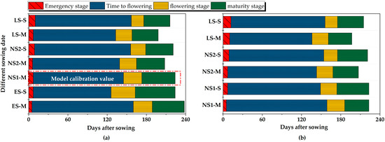
Figure 4.
(a) Days of different phenological stages in 2020 growing season, (b) days of different phenological stages in 2021 growing season. S: Simulated value of phenological days, M: measured value of phenological days.
In a comparison of the fixed growth days simulation with the calendar mode, the GDD model achieved a similar trend. Therefore, we choose the GDD model to simulate and set the accumulated temperature from sowing to maturity as the calibration value as the basic threshold. This indicated that under this mode, the beginning and ending of each growth stage were tightly controlled by the GDD values. With the delay of the sowing date, the growth days of rapeseed were shortened, indicating that the total GDD of rapeseed was changed [15,45]. Therefore, the model had the deviation in simulating phenological days for different sowing dates. Shortening of the growth period was mainly affected by photoperiod and temperature. Nanda et al. [47] pointed out that the growth period of rapeseed before flowering was mainly affected by the photoperiod, while the flowering duration of rapeseed was mainly controlled by the temperature. The growth process of rapeseed was accelerated with the increase of the photoperiod. A similar conclusion was also reported when investigating the effects of sowing dates on maize by Cai et al. [48]. The experiment dates showed that the time to flowering for rapeseed was shortened by 5–29 days with the delay of the sowing date, and the flowering duration was stable at about 27 days. Therefore, with the delay of the sowing date, the total GDD required for rapeseed to reach maturity would be decreased. The model uses a unified GDD threshold in the simulation of rapeseed growth for different sowing dates (Table 2). For example, the time node to the flowering stage in the simulation of all sowing dates of the GDD of 1437 °C was used as the threshold for the time to flowering stage, which resulted in the simulated values of the LS and NS2 treatments being significantly shorter than the measured values in two growing seasons, while in the ES treatment, the simulated values were lower than the measured values.
3.2. Canopy Cover
CC is one of the important driving and output variables in the AquaCrop model and an accurate estimation of crop canopy cover is crucial for determining the simulation results of ETC, biomass and yield. Comparisons of simulated and measured canopy coverage at different sowing dates is shown in Figure 5. The simulation results in two growing seasons showed that the simulated winter rapeseed coverage was in good agreement with the measured values. The simulation accuracy of rapeseed CC in 2020 (RMSE: 7–21%; EF: 0.54–0.95; R2: 0.79–0.97) was better than of that in 2021 (RMSE: 13–22%; EF: 0.55–0.83; R2: 0.70–0.89). Generally, the simulation accuracies of the CC were gradually improved with the postponement of sowing dates. A common feature was observed in both seasons whereby a peak or a short platform period was observed at 60–120 days after sowing (DAS), and then continued to rise to the maximum CC until maturity. Compared with the later sowing dates treatment, the average temperature of the seedling stage for the ES and NS1 sowing dates treatments were 18–24 °C, which were further beyond the threshold of the base temperature (0 °C). Therefore, a higher temperature promoted rapeseed to develop more rapidly in the vegetative growth stage of the seedling stage and an abundance of leaves was produced, resulting in the surface coverage to increase rapidly. With the delay of the sowing date, the monthly average temperature of NS2 and LS decreased to 4–13 °C, triggering a low temperature stress that limited rapeseed development. Compared with the high coverage caused by the rapid development of leaves before the wintering of ES and NS1, NS2 and LS maintained a low coverage in winter before entering the reproductive growth stage, resulting in a flat trend of the measured data [31,49,50]. In addition, 2021-NS1-HD maintained a low coverage in the early growth stage. This is due to the comparison of 20 mm rainfall in 60 DAS after 2020-NS1 sowing, and 151 mm rainfall in 60 DAS after 2021-NS1 sowing. Excessive water limits the development of the rapeseed canopy. Waterlogging is one of the reasons that the growth and development of rapeseed is limited, leading to a yield reduction, through the study of Cong et al. [51].
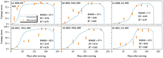
Figure 5.
Simulated and measured canopy cover for different sowing dates in 2020 (a–c) and 2021 (d–f) growing seasons (The different sowing date scenarios were verified under HD density).
Comparisons of the simulated and measured canopy coverage at different densities is shown in Figure 6. In the 2020 growing season, the simulation accuracy decreased as the density lowered (RMSE: 12–23%; EF: 0.81–0.50; R2: 0.89–0.69). Meanwhile, it can be seen that the measured CC values of the density treatment were significantly higher than that of the model simulation value during the 0–90 DAS in 2020 growing season. The main reason could be attributed to the rapid development of the NS1 treatment in the vegetative stage of the seedling stage, and the larger leaves of rapeseed triggered the surface coverage to increase rapidly. With the ending of the overwintering period of rapeseed, the early developed leaves began to wither with the development of stems and lateral branches, and the LD treatment CC decreased significantly compared with other density treatments. The same situation occurred in the 2021 growing season, although the early development of the 2021-NS1 canopy was subjected to water stress resulting in lower CC measurements. The HD treatment coverage was 10% higher than the LD treatment regarding rapeseed development after overwintering (90 DAS). Compared with the large fluctuation of measured values in the two growing seasons, the simulated values of CC were more consistent. This was because the GDD threshold used by the model to simulate the time for the rapeseed maximum canopy at different sowing densities is fixed. In this study, there were three maximum coverages (HD: 95%, MD: 90%, LD: 85%) for different densities, resulting in the decrease for the growth rate of the curve. The calibrated AquaCrop is acceptable for the simulation accuracy of winter rapeseed CC in the region by comparison with the results (average RMSE: 27%; EF: 0.61. R2: 0.82) of Dirwai and Zeleke et al. [38,39].
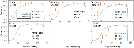
Figure 6.
Simulated and measured canopy cover for different sowing densities in 2020 (a–c) and 2021 (d,e) growing seasons (the verification of different density scenarios was performed under NS1 sowing date conditions).
3.3. Crop Evapotranspiration
The ETC simulation accuracies of the different densities (RMSE: 19 mm) were higher than those of the different sowing dates (RMSE: 31 mm). In Figure 6, it can be seen that the simulated ETC under different sowing densities were divided into two parts: 393 mm and 434 mm. The main reason was that the simulation results of the soil moisture were consistent when the different seeding densities were simulated under the condition of the same seeding time, so the simulated ETC calculated according to the water balance equation was the same. Therefore, when verified in different density scenarios during the 2020 growing season, the ETC for the three density treatments were 393 mm. This indicated that the model does not consider the effects of sowing density and maximum canopy cover changes when simulating soil moisture conditions during the same sowing period. The same situation was reported In the study of Sanhu et al. [10]. Notably, two points were deviated from the simulation of different sowing dates, namely 2020-ES and 2020-LS (Figure 7). The reason could be attributed to the errors in the model estimation of the phenological days mentioned in Section 3.1. For the ES treatment, the length of growth days was underestimated by 14 days, in which the precipitation of 129 mm was observed, resulting in a bias in calculating the measured ETc. Additionally, the length of growth days of the LS treatment was overestimated by 18 days, inducing an overestimated error of the ETc. Although the total growth lengths of NS2 and NS1 were also overestimated by 14–18 days in the model simulation, only 1–9.6 mm rainfall were recorded during the period, which has no significant impact on the ETc estimation.
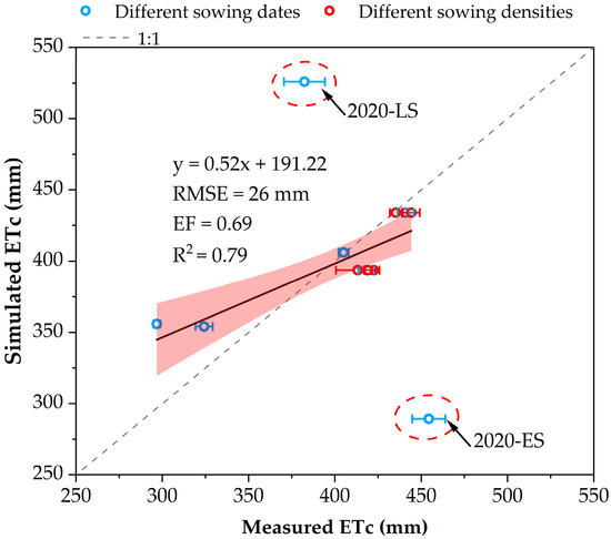
Figure 7.
Simulated and measured ETC for all treatments in 2020 and 2021 growing seasons. (The different sowing date scenarios were verified under HD density conditions. The validation of different density scenarios was performed under NS1 sowing date conditions).
In general, compared with the results obtained by Raja and Sandhu et al. [10,52], who used the AquaCrop model to simulate maize at different planting dates and densities (whole RMSE: 17 and 35 mm, R2: 0.71 and 0.54), the AquaCrop model has the adaptable performance for estimating the ETC of winter rapeseed (whole RMSE: 26 mm, EF: 0.69, R2: 0.79).
3.4. Biomass and Grain Yield
The simulated results of biomass and yield were in good agreement with the measurements in the different sowing date treatments. The simulation accuracy of biomass in the 2020 growing season (RMSE: 0.8–1.7 ton·ha−1; EF: 0.72–0.96; R2: 0.92–0.99) was generally higher than that in 2021 growing season (RMSE: 1.4–2.1 ton·ha−1; EF: 0.71–0.89; R2: 0.94–0.97). The main reason for the lower accuracy in the second year could be attributed to the limitation of early canopy development (Figure 5 and Figure 6), which decreased the canopy transpiration (Tr) and triggered a lower cumulative dry matter mass.
The biomass simulation results for the different densities are shown in Figure 8. In 2020-NS1, the biomass of the HD and MD treatments achieved good simulation results (EF: 0.91–0.92, RMSE: 1.25–1.55 t·ha−1). As mentioned earlier, 2021-NS1-HD was limited in its simulation accuracy due to early canopy development (EF: 0.71, RMSE: 2.1 t·ha−1). In the biomass simulation of low density, more than 40% overestimations were observed in both growing seasons (Figure 9c,e). Although the maximum canopy cover of differentiation for the sowing densities were arranged (85%, 90% and 95%), these canopy cover differences were not significant for the change of biomass accumulation based on model mechanisms (Equation (3)). One possibility to solve this problem is to adjust the WP* by establishing a correlation with the sowing densities. Based on the two years of field experiment data, Li et al. [15] reported that rational close planting helps to increase rapeseed crop yields.
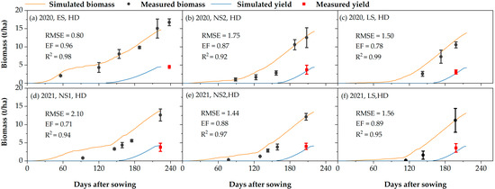
Figure 8.
Simulated and measured biomass for different sowing dates in 2020 (a–c) and 2021 (d–f) growing seasons.
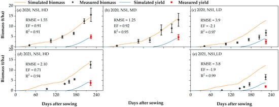
Figure 9.
Simulated and measured biomass for different sowing densities in 2020 (a–c) and 2021 (d,e) growing seasons.
Table 3 displays the yield simulation for different sowing dates and density treatments. For the different sowing date treatments, the simulated yield presented a general overestimation but had a large fluctuation in both seasons, with the Pe ranging from 0–35.3%. In the GDD-driven mode, the comparison in yields between those simulated and measured were not only in final values, but in harvest time. For instance, although the relative error of yield was 0% in the simulated ES treatment, the simulated harvest date was ahead of the actual harvest time. At the opposite of early sowing, the overestimation error observed in the NS2 and LS treatments are mainly attributed to the delay of simulation maturity times (Figure 8 and Table 3). The simulation results of the yield under different densities were consistent with the dry biomass simulation where good agreement was achieved for the HD and MD treatments, with the maximum Pe around 10%. On the other hand, the underestimated biomass brought a low production, resulting in the simulation accuracy being unacceptable. Comparable results were also reported by Dirwai et al. [39], who suggested that the simulation accuracy of rapeseed biomass and yield using AquaCrop was adequate, with the EF ranging from 0.30 to 0.54 and Pe from 34% to 58%. Nevertheless, the AquaCrop model provided sufficient accuracy for the simulation of a high-density rapeseed yield.
Table 3.
Comparison between final yield simulated and measured values (the different sowing date scenarios were verified under HD density conditions, and the different density scenarios were performed under NS1 sowing date conditions).
3.5. Optimum Sowing Date and Density
As the main factors of rapeseed yields, the sowing date and density will change with the change of region and climatic conditions. Therefore, it is important to explore the optimal sowing date and density for the formulation of local production management measures and the improvement of rapeseed yields [53]. The comparison of in situ measured yields for all treatments in both growing seasons are shown in Table 4. In the 2020 growing season, with the increase of density, the yield of rapeseed was increased. With the exception of the ES treatment, the yield of the LD treatment was significantly lower than that of the MD and HD treatments, while the differences between the MD and HD treatments were not obvious. Furthermore, the yield would decline with the delay of the sowing date. During the 2021 growing season, this conclusion was confirmed. Appropriate sowing dates and a reasonable sowing density could effectively increase the winter rapeseed yield. The conclusion was consistent with the yield simulation results of the AquaCrop model in Section 3.4 and similar results were also reported by Li et al. [15].
Table 4.
All treatments grain yields in the 2020 and 2021 growing seasons.
The early sowing rapeseed has a higher accumulation dry matter before entering the overwintering stage than that of the late sowing scenarios. With the rapeseed reviving after the overwintering period, the growth process would be accelerated with the increase of the photoperiod; thus, the late sowing rapeseed in the vegetative stage of the dry matter accumulation time was insufficient [47,54]. The same conclusion was reported in a study of the effects of sowing dates on dry matter accumulation in rice and maize by Pal and Fu et al. [48,55]. Meanwhile, the study also mentioned that the delay of the sowing date would shorten the growth of crops, which mainly occurred in the vegetative growth stage (from emergence to jointing). Although late-sowing rapeseed had the same cultivation and management as early-sowing winter rapeseed, it could not obtain a higher yield. This shows that for an increase of winter rapeseed yields, an earlier sowing date should be chosen, so that winter rapeseed has sufficient dry matter accumulation. Meanwhile, with an increase of the rapeseed sowing density, canopy light use efficiency and effective pod numbers, higher crop canopy coverage and decrease of the soil evaporation, the yield was increased [56,57,58]. Therefore, combined with the measured data and simulated results of the rapeseed, an optimal sowing date in October and sowing density of around 25.0–37.5 plant·m−2 in the Jianghuai Plain would achieve a steadily high yield.
4. Conclusions
This study revealed the response of rapeseed growth under various sowing dates and densities conditions, evaluated the capability of the AquaCrop model for interpreting the variation of simulated phenological dates, canopy coverage, biomass, yield and evapotranspiration and determined the optimal sowing date and density of winter rapeseed in the Jianghuai Plain.
With the delay of the sowing date, the growth period of rapeseed was shortened (from 238 days to 197 days) and the yield was reduced (from 4.9 t·ha−1 to 3.1 t·ha−1). Due to the influence of the change of the sowing date on the growth cycle of rapeseed, the estimation of phenological days in the model has a deviation of 1–18 days. The difference in rapeseed yields between the NS1-HD and LS-HD treatments reached 3.15 t·ha−1 in 2020. Meanwhile, the rapeseed yield was significantly increased with the increase of sowing density. The simulated CC achieved satisfactory accuracy in different sowing dates scenarios (RMSE: 7–22%; EF: 0.54–0.95: R2: 0.70–0.97). The estimated ETC of winter rapeseed were in good agreement with the in situ measurement, with the R2, RMSE and EF of 0.79, 26 mm, and 0.69, respectively. In the simulation of biomass and yield, the medium- and high-density treatments achieved higher simulation accuracy (RMSE: 0.8–2.1 t·ha−1, EF: 0.71–0.96, Pe: 0–35%). The model overestimated the rapeseed production potential in the LD condition (about 40%). Combined with the measured data and simulated results of the rapeseed, an optimal sowing date in October and a sowing density of around 25.0–37.5 plant·m−2 in the Jianghuai Plain would achieve a steadily high yield.
The study demonstrates the great potential of the AquaCrop model for optimal rapeseed sowing patterns and provides technical means guidance for the formulation of local winter rapeseed production. Despite the encouraging results, further improvements are warranted to solve the overestimation problem in low density production, such as adjustments to water productivity or the harvest index.
Author Contributions
Writing—original draft preparation, Z.X.; methodology, J.K. and D.L.; writing—review and editing, C.Z. and M.T.; data curation, Z.L. and R.L.; funding acquisition, C.Z. and S.F. All authors have read and agreed to the published version of the manuscript.
Funding
This research was funded by the National Natural Science Foundation of China (51909228, 52209071), and the project was funded by the Postdoctoral Science Foundation of China (2020M671623), and the “Blue Project” of Yangzhou University.
Data Availability Statement
The data that support this study cannot be publicly shared due to ethical or privacy reasons and may be shared upon reasonable request to the corresponding author if appropriate.
Acknowledgments
The authors would like to acknowledge the agricultural water and hydrological ecology experiment station, Yangzhou University for providing the experiment facilities.
Conflicts of Interest
The authors declare no conflict of interest.
References
- Wang, H.; Yin, Y. Analysis and strategy for oil crop industry in China. Chin. J. Oil Crop Sci. 2014, 36, 414–421. [Google Scholar]
- National Bureau of Statistics of China. China Statistical Yearbook; China Statistical Press: Beijing, China, 2021. Available online: www.stats.gov.cn (accessed on 1 June 2022).
- Wang, H.; Chen, X.; Hu, F. Adaptative adjustments of the sowing date of late season rice under climate change in Guangdong Province. ACTA Ecol. Sin. 2011, 15, 4261–4269. [Google Scholar]
- Ozer, H. Sowing date and nitrogen rate effects on growth, yield and yield components of two summer rapeseed cultivars. Eur. J. Agron. 2003, 19, 453–463. [Google Scholar] [CrossRef]
- Weymann, W.; Böttcher, U.; Sieling, K.; Kage, H. Effects of weather conditions during different growth phases on yield formation of winter oilseed rape. Field Crops Res. 2015, 173, 41–48. [Google Scholar] [CrossRef]
- Kirkegaard, J.; Lilley, J.; Brill, R.; Sprague, S.; Fettell, N.; Pengilley, G. Re-evaluating sowing time of spring canola (Brassica napus L.) in south-eastern Australia—How early is too early? Crop Pasture Sci. 2016, 67, 381–396. [Google Scholar] [CrossRef]
- Mao, L.; Zhang, L.; Zhao, X.; Liu, S.; van der Werf, W.; Zhang, S.; Spiertz, H.; Li, Z. Crop growth, light utilization and yield of relay intercropped cotton as affected by plant density and a plant growth regulator. Field Crops Res. 2014, 155, 67–76. [Google Scholar] [CrossRef]
- McGregor, D. Effect of plant density on development and yield of rapeseed and its significance to recovery from hail injury. Can. J. Plant Sci. 1987, 67, 43–51. [Google Scholar] [CrossRef]
- Griesh, M.; Yakout, G. Effect of plant population density and nitrogen fertilization on yield and yield components of some white and yellow maize hybrids under drip irrigation system in sandy soil. In Plant Nutrition; Springer: Berlin/Heidelberg, Germany, 2001; pp. 810–811. [Google Scholar]
- Sandhu, R.; Irmak, S. Assessment of AquaCrop model in simulating maize canopy cover, soil-water, evapotranspiration, yield, and water productivity for different planting dates and densities under irrigated and rainfed conditions. Agric. Water Manag. 2019, 224, 105753. [Google Scholar] [CrossRef]
- Al-Doori, S.A.M. A study of the importance of sowing dates and plant density affecting some rapeseed cultivars (Brassica napus L.). Coll. Basic Educ. Res. J. 2011, 11, 615–632. [Google Scholar]
- Vincze, E. The effect of sowing date and plant density on yield elements of different winter oilseed rape (Brassica napus var. napus f. biennis L.) genotypes. Columella J. Agric. Environ. Sci. 2017, 4, 21–25. [Google Scholar]
- Gusta, L.; Johnson, E.; Nesbitt, N.; Kirkland, K. Effect of seeding date on canola seed quality and seed vigour. Can. J. Plant Sci. 2004, 84, 463–471. [Google Scholar] [CrossRef]
- Guan, C.; Chen, S. Investigation on planting density of double low rapeseed “Xiangyou 15”. Crop Res. 2003, 17, 136–137. [Google Scholar]
- Li, X.; Zuo, Q.; Chang, H.; Bai, G.; Kuai, J.; Zhou, G. Higher density planting benefits mechanical harvesting of rapeseed in the Yangtze River Basin of China. Field Crops Res. 2018, 218, 97–105. [Google Scholar] [CrossRef]
- He, D.; Wang, E.; Wang, J.; Robertson, M.J. Data requirement for effective calibration of process-based crop models. Agric. For. Meteorol. 2017, 234, 136–148. [Google Scholar] [CrossRef]
- ur Rahman, M.H.; Ahmad, A.; Wang, X.; Wajid, A.; Nasim, W.; Hussain, M.; Ahmad, B.; Ahmad, I.; Ali, Z.; Ishaque, W. Multi-model projections of future climate and climate change impacts uncertainty assessment for cotton production in Pakistan. Agric. For. Meteorol. 2018, 253, 94–113. [Google Scholar] [CrossRef]
- Rodriguez, D.; De Voil, P.; Hudson, D.; Brown, J.; Hayman, P.; Marrou, H.; Meinke, H. Predicting optimum crop designs using crop models and seasonal climate forecasts. Sci. Rep. 2018, 8, 2231. [Google Scholar] [CrossRef] [PubMed]
- Nunes, H.; Farias, V.; Sousa, D.; Costa, D.; Pinto, J.; Moura, V.; Teixeira, E.; Lima, M.; Ortega-Farias, S.; Souza, P. Parameterization of the AquaCrop model for cowpea and assessing the impact of sowing dates normally used on yield. Agric. Water Manag. 2021, 252, 106880. [Google Scholar] [CrossRef]
- Chen, S.; Jiang, T.; Ma, H.; He, C.; Xu, F.; Malone, R.W.; Feng, H.; Yu, Q.; Siddique, K.H.; He, J. Dynamic within-season irrigation scheduling for maize production in Northwest China: A Method Based on Weather Data Fusion and yield prediction by DSSAT. Agric. For. Meteorol. 2020, 285, 107928. [Google Scholar] [CrossRef]
- Zadeh, S.F.M.; Honar, T.; Rahmati, H. Simulation of Seed Yield and Dry Matter of Canola Under The Condition of Water Stress Using SWAP Model. Irrig. Sci. Eng. 1970, 40, 153–165. [Google Scholar]
- Jing, Q.; Shang, J.; Qian, B.; Hoogenboom, G.; Huffman, T.; Liu, J.; Ma, B.L.; Geng, X.; Jiao, X.; Kovacs, J.; et al. Evaluation of the CSM-CROPGRO-Canola Model for Simulating Canola Growth and Yield at West Nipissing in Eastern Canada. Agron. J. 2016, 108, 575–584. [Google Scholar] [CrossRef]
- He, D.; Wang, E.; Wang, J.; Lilley, J.; Luo, Z.; Pan, X.; Pan, Z.; Yang, N. Uncertainty in canola phenology modelling induced by cultivar parameterization and its impact on simulated yield. Agric. For. Meteorol. 2017, 232, 163–175. [Google Scholar] [CrossRef]
- Qian, B.; Jing, Q.; Zhang, X.; Shang, J.; Liu, J.; Wan, H.; Dong, T.; De Jong, R. Adapting estimation methods of daily solar radiation for crop modelling applications in Canada. Can. J. Soil Sci. 2019, 99, 533–547. [Google Scholar] [CrossRef]
- Abedinpour, M.; Sarangi, A.; Rajput, T.; Singh, M.; Pathak, H.; Ahmad, T. Performance evaluation of AquaCrop model for maize crop in a semi-arid environment. Agric. Water Manag. 2012, 110, 55–66. [Google Scholar] [CrossRef]
- Toumi, J.; Er-Raki, S.; Ezzahar, J.; Khabba, S.; Jarlan, L.; Chehbouni, A. Performance assessment of AquaCrop model for estimating evapotranspiration, soil water content and grain yield of winter wheat in Tensift Al Haouz (Morocco): Application to irrigation management. Agric. Water Manag. 2016, 163, 219–235. [Google Scholar] [CrossRef]
- Steduto, P.; Raes, D.; Hsiao, T.C.; Fereres, E.; Heng, L.K.; Howell, T.A. Concepts and applications of AquaCrop: The FAO crop water productivity model. In Crop Modeling and Decision Aupport; Springer: Berlin/Heidelberg, Germany, 2009; pp. 175–191. [Google Scholar]
- Katerji, N.; Campi, P.; Mastrorilli, M. Productivity, evapotranspiration, and water use efficiency of corn and tomato crops simulated by AquaCrop under contrasting water stress conditions in the Mediterranean region. Agric. Water Manag. 2013, 130, 14–26. [Google Scholar] [CrossRef]
- Steduto, P.; Hsiao, T.C.; Raes, D.; Fereres, E. AquaCrop—The FAO crop model to simulate yield response to water: I. Concepts and underlying principles. Agron. J. 2009, 101, 426–437. [Google Scholar] [CrossRef]
- Sun, S.; Zhang, L.; Chen, Z.; Sun, J. Advances in AquaCrop model research and application. Sci. Agric. Sin. 2017, 50, 3286–3299. [Google Scholar]
- Zhang, C.; Xie, Z.; Shang, J.; Liu, J.; Dong, T.; Tang, M.; Feng, S.; Cai, H. Detecting winter canola (Brassica napus) phenological stages using an improved shape-model method based on time-series UAV spectral data. Crop J. 2022, 10, 1353–1362. [Google Scholar] [CrossRef]
- Purevdorj, T.; Tateishi, R.; Ishiyama, T.; Honda, Y. Relationships between percent vegetation cover and vegetation indices. Int. J. Remote Sens. 1998, 19, 3519–3535. [Google Scholar] [CrossRef]
- Jiapaer, G.; Chen, X.; Bao, A. A comparison of methods for estimating fractional vegetation cover in arid regions. Agric. For. Meteorol. 2011, 151, 1698–1710. [Google Scholar] [CrossRef]
- Niu, Y.; Zhang, L.; Han, W.; Shao, G. Fractional vegetation cover extraction method of winter wheat based on UAV remote sensing and vegetation index. Trans. CSAM 2018, 49, 213–221. [Google Scholar]
- Allen, R.G.; Pereira, L.S.; Raes, D.; Smith, M. Crop Evapotranspiration-Guidelines for Computing Crop Water Requirements-FAO Irrigation and Drainage Paper 56; Fao: Rome, Italy, 1998; Volume 300, p. D05109. [Google Scholar]
- Doorenbos, J.; Kassam, A. Yield response to water. In Irrigation and Drainage Paper; Elsevier: Amsterdam, The Netherlands, 1979; Volume 33, p. 257. [Google Scholar]
- Steduto, P.; Hsiao, T.C.; Fereres, E. On the conservative behavior of biomass water productivity. Irrig. Sci. 2007, 25, 189–207. [Google Scholar] [CrossRef]
- Zeleke, K.T.; Luckett, D.; Cowley, R. Calibration and Testing of the FAO AquaCrop Model for Canola. Agron. J. 2011, 103, 1610–1618. [Google Scholar] [CrossRef]
- Dirwai, T.L.; Senzanje, A.; Mabhaudhi, T. Calibration and Evaluation of the FAO AquaCrop Model for Canola (Brassica napus) under Varied Moistube Irrigation Regimes. Agriculture 2021, 11, 410. [Google Scholar] [CrossRef]
- Zhou, M.; Ma, X.; Wang, K.; Cheng, T.; Tian, Y.; Wang, J.; Zhu, Y.; Hu, Y.; Niu, Q.; Gui, L.; et al. Detection of phenology using an improved shape model on time-series vegetation index in wheat. Comput. Electron. Agric. Comput. Electron. Agric. 2020, 173, 105398. [Google Scholar] [CrossRef]
- Mandal, D.; Kumar, V.; Ratha, D.; Dey, S.; Bhattacharya, A.; Lopez-Sanchez, J.M.; McNairn, H.; Rao, Y.S. Dual polarimetric radar vegetation index for crop growth monitoring using sentinel-1 SAR data. Remote Sens. Environ. 2020, 247, 111954. [Google Scholar] [CrossRef]
- Schlund, M.; Erasmi, S. Sentinel-1 time series data for monitoring the phenology of winter wheat. Remote Sens. Environ. 2020, 246, 111814. [Google Scholar] [CrossRef]
- Harker, K.; O’Donovan, J.; Smith, E.; Johnson, E.; Peng, G.; Willenborg, C.; Gulden, R.; Mohr, R.; Gill, K.; Grenkow, L. Seed size and seeding rate effects on canola emergence, development, yield and seed weight. Can. J. Plant Sci. 2015, 95, 1–8. [Google Scholar] [CrossRef]
- Shah, S.; Akmal, M. Effect of different sowing date on yield and yield components of wheat varieties. Sarhad J. Agric. 2002, 1016, 4383. [Google Scholar] [CrossRef]
- Jiang, H.; Sun, W.; Zeng, X.; Chen, J.; Shi, P.; Zhao, C.; Li, H. Effect of sowing date on Brassica rape growth and yield in northern China. Chin. J. Oil Crop Sci. 2012, 34, 6. [Google Scholar]
- Serafin-Andrzejewska, M.; Helios, W.; Jama-Rodzeńska, A.; Kozak, M.; Kotecki, A.; Kuchar, L. Effect of Sowing Date on Soybean Development in South-Western Poland. Agriculture 2021, 11, 413. [Google Scholar] [CrossRef]
- Nanda, R.; Bhargava, S.; Tomar, D.; Rawson, H. Phenological development of Brassica campestris, B. juncea, B. napus and B. carinata grown in controlled environments and from 14 sowing dates in the field. Field Crops Res. 1996, 46, 93–103. [Google Scholar] [CrossRef]
- Cai, F.; Zhang, Y.; Mi, N.; Ming, H.; Zhang, S.; Zhang, H.; Zhao, X.; Zhang, B. The Effect of Drought and Sowing Date on Dry Matter Accumulation and Partitioning in the Above-Ground Organs of Maize. Atmosphere 2022, 13, 677. [Google Scholar] [CrossRef]
- Sun, W.; Wu, J.; Fang, Y.; Liu, Q.; Yang, R.; Ma, W.; Li, X.; Zhang, J.; Zhang, P.; Lei, J. Growth and development characteristics of winter rapeseed northern-extended from the cold and arid regions in China. Acta Agron. Sin. 2010, 36, 2124–2134. [Google Scholar] [CrossRef]
- Guan, C.; Jin, F.; Dong, G.; Guan, M.; Tan, T. Exploring the growth and development properties of early variety of winter rapeseed. Eng. Sci. 2012, 14, 4–12. [Google Scholar]
- Cong, R.; Zhang, Z.; Lu, J. Climate impacts on yield of winter oilseed rape in different growth regions of the Yangtze River Basin. Chin. J. Oil Crop Sci. 2019, 41, 894. [Google Scholar]
- Raja, W.; Kanth, R.H.; Singh, P. Validating the AquaCrop model for maize under different sowing dates. Water Policy 2018, 20, 826–840. [Google Scholar] [CrossRef]
- Begna, S.H.; Angadi, S.V. Effects of planting date on winter canola growth and yield in the southwestern US. Am. J. Plant Sci. 2016, 7, 201–217. [Google Scholar] [CrossRef]
- Li, G.; Guan, C. Study on characteristics of dry matter accumulation, distribution and transfer of winter rapeseed (Brassica napus). Zuo Wu Xue Bao 2002, 28, 52–58. [Google Scholar]
- Pal, R.; Mahajan, G.; Sardana, V.; Chauhan, B. Impact of sowing date on yield, dry matter and nitrogen accumulation, and nitrogen translocation in dry-seeded rice in North-West India. Field Crops Res. 2017, 206, 138–148. [Google Scholar] [CrossRef]
- Wang, R.; Cheng, T.; Hu, L. Effect of wide–narrow row arrangement and plant density on yield and radiation use efficiency of mechanized direct-seeded canola in Central China. Field Crops Res. 2015, 172, 42–52. [Google Scholar] [CrossRef]
- Harker, K.; O’Donovan, J.; Blackshaw, R.; Johnson, E.; Lafond, G.; May, W. Seeding depth and seeding speed effects on no-till canola emergence, maturity, yield and seed quality. Can. J. Plant Sci. 2012, 92, 795–802. [Google Scholar] [CrossRef]
- Jabran, K.; Cheema, Z.; Farooq, M.; Hussain, M. Lower doses of pendimethalin mixed with allelopathic crop water extracts for weed management in canola (Brassica napus). Int. J. Agric. Biol. 2010, 12, 335–340. [Google Scholar]


Disclaimer/Publisher’s Note: The statements, opinions and data contained in all publications are solely those of the individual author(s) and contributor(s) and not of MDPI and/or the editor(s). MDPI and/or the editor(s) disclaim responsibility for any injury to people or property resulting from any ideas, methods, instructions or products referred to in the content. |
© 2023 by the authors. Licensee MDPI, Basel, Switzerland. This article is an open access article distributed under the terms and conditions of the Creative Commons Attribution (CC BY) license (https://creativecommons.org/licenses/by/4.0/).