Abstract
Soil total nitrogen is one of the most important basic indicators for fertiliser decision making, but tens of millions of soil total nitrogen sampling data have been accumulated, forming a huge database. In this large database, there is a large amount of anomalous data, which can interfere with data analysis, affect the construction of spatial interpolation and prediction models, and then affect the accuracy of nutrient management decisions. The traditional method of identifying soil total nitrogen anomalies based on boxplots suffers from the problems of not being able to identify local anomalies, which can easily lead to misclassification of soil total nitrogen data anomalies, and the detection efficiency is not high. We propose a method to identify soil total nitrogen outliers by combining the Isolation Forest algorithm and local spatial autocorrelation analysis, which can simultaneously detect global and local outliers from large amounts of data and combine organic matter as an auxiliary indicator in the spatial analysis to help judge local outliers. Finally, the results of global and local anomalies were combined to provide a comprehensive assessment of the soil nitrogen data, avoiding the misjudgement or omission of judgement that can occur when using a single method. Using 25,930 soil test data from Yunnan Province in 2009 as an example, we compared and analysed the typical boxplot method and the unsupervised OneClassSVM method and evaluated the performance of each method in terms of correct detection rate, false positive rate and false negative rate. The results show that the proposed method has a correct detection rate (TR) of 99.97%, a false positive rate (FPR) of 8.06% and a false negative rate (FNR) of 0.01% on the data, which shows high validity and accuracy; it is also comparable to the independent isolated forests (FNR = 4.76%), boxplot (FNR = 3.90%) and OneClassSVM (FNR = 4.77%), and the false negative rate is reduced by 4.75%, 3.89% and 4.76%, respectively.
1. Introduction
Soil total nitrogen is the sum of the different forms of nitrogen in the soil, including organic and inorganic nitrogen [1], and is an important nutrient affecting grain yield and quality, with too much or too little nitrogen being detrimental to crop production [2,3]. Soil total nitrogen is usually determined by micro-Kjeldahl, semi-micro-Kjeldahl and micro-potassium sulphate methods [4], and the results can provide an important basis for soil formulation and fertiliser application, help improve nitrogen fertiliser use and reduce pollution of agricultural surface water sources [5]. However, due to the complexity and diversity of agricultural production conditions, a variety of soil types and soil nutrient distribution variations, in the large-scale soil nutrient data collection, experimental procedures, input, transmission and other links are likely to be errors or breakdowns [6] in nature or human factors that may also cause real but rare or sudden changes [7]. These problems lead to the presence of outliers in soil test data, and these outliers can distort the spatial distribution pattern of soil total nitrogen data, affecting spatial interpolation and predictive modelling, resulting in fertiliser application decisions based on incorrect soil total nitrogen information, which may lead to under- or over-application of nutrients and consequently affect crop growth and yield. This can reduce the efficiency of agricultural production and even have a negative impact on the environment. The detection and identification of outliers is therefore an important prerequisite and basis for data analysis and modelling. In the analysis and processing of soil test data, there is an urgent need for a more efficient and accurate method of detecting soil total nitrogen (TN) outliers, improving TN data quality and reducing data errors to better support fertiliser application decisions and nutrient management practices.
Currently, the main methods for detecting spatial outliers include statistical methods and spatial autocorrelation methods, but the widely accepted best method has not yet been developed [8]. The main statistical methods are t-test, Grubbs, Dixon, Walsh and standard deviation range [9]. Among the most commonly used methods are the use of boxplots to identify outliers [8] and the use of the triple standard deviation range method to identify outliers [10]. These methods require a high distribution pattern of the dataset and can only detect global anomalies, failing to fully account for the spatial autocorrelation of TN data, and therefore cannot effectively detect local outliers of TN [11]. In particular, due to the massive nature of TN data, existing methods face challenges in dealing with this issue. Spatial autocorrelation methods are divided into global spatial autocorrelation and local spatial autocorrelation, and local spatial autocorrelation analysis can determine whether the datum is an outlier or not based on the similarity between observations and neighbouring observations [12]. Among them, local indicators of spatial association (LISA) are a commonly used method in spatial anomaly detection [13]. For example, Zhang et al. used Local Moran’s I to identify Pb contamination in urban soils and found the effects of data transformation and extreme values on data analysis [14]; Yuan et al. also used Local Moran’s I to identify REE contamination in soils [15]. Currently, local spatial autocorrelation analysis is widely used in spatial data anomaly detection [16,17], which helps to reveal local anomalies in datasets. In addition, with the rapid development of artificial intelligence technology, machine learning has obvious advantages in data processing and analysis, which can handle large and complex datasets, and has been widely applied in outlier detection in the fields of finance, manufacturing and healthcare [18,19]. For example, Orlova et al. used hierarchical clustering, k-mean and gradient-boosting algorithms to construct clustering and classification models for credit scoring and risk prediction of borrowers [20]; Orlova et al. analysed the application of k-mean and support vector machine algorithms in the management of production labour rate in the enterprise [21]; and Li et al. used AI algorithms to predict groundwater depth [22]. Among them, the Isolation Forest algorithm is an unsupervised outlier detection algorithm based on the idea of integrated learning and random forests [23], which uses an isolation mechanism to detect anomalies, and has high speed and accuracy in identifying global outliers but is less sensitive to local outliers [24]. Therefore, the combination of machine-learning algorithms and local spatial autocorrelation analysis in spatial data outlier detection can combine the advantages of global and local outlier detection in big data, which can improve the accuracy of outlier identification and reduce the misclassification of correct data.
Considering the characteristics of TN data and the shortcomings of existing methods, this study proposes to identify the global outliers of TN using the Isolation Forest algorithm, identify the local outliers of TN using local spatial autocorrelation and combine this with other soil nutrient indices to perform the auxiliary discrimination of local outliers, and finally, the results of Isolation Forest and local spatial autocorrelation are used to jointly discriminate the outliers of TN. This study compared and analysed the method with other commonly used methods using soil test data from Yunnan Province in 2009 as an example and evaluated the performance of each method in terms of correct detection rate, false positive rate and false negative rate. The objectives of this study were (1) to analyse the data characteristics of the five basic soil nutrient test data in Yunnan Province in 2009, (2) to evaluate the performance of the proposed TN outlier identification model, (3) to compare the accuracy of different methods for identifying TN outliers and (4) to analyse the characteristics of soil total nitrogen distribution in Yunnan Province. The proposed method provides a new idea and method for identifying TN outliers and supports soil nutrient analysis and assessment.
2. Materials and Methods
The data were obtained from the 2009 soil survey data in Yunnan Province and included information on total soil nitrogen, organic matter, pH, available phosphorus, available potassium and spatial location. The dataset contains 25,930 observations and the following pre-processing steps were carried out to improve the quality and usability of the data:
- (1)
- Removal of missing and duplicate values. The Pandas library in the Python language was used to clean the data, and all observation records with missing or duplicate values were removed to ensure the integrity and uniqueness of the data.
- (2)
- Statistical analysis. The Python language was used to perform routine statistical analyses of the data to gain a fuller understanding of the characteristics and trends of the data.
- (3)
- Box–Cox transformation of the data to approximate a normal distribution. As the distribution of soil nutrient indicators may be skewed or peaked, which does not conform to the normality assumption of most statistical analysis methods, this study used Box–Cox regression in STATA to perform a Box–Cox transformation on the data, which can be used to find the appropriate parameters according to the characteristics of the data, making the transformed data more in line with the normal distribution [25].
- (4)
- Spatial interpolation of data to produce spatial-distribution maps. As the raw data were based on point samples from different locations, which could not visually reflect the spatial distribution of soil nutrients across the region, this study carried out spatial interpolation using the inverse distance weighting method in the spatial analysis tool of ArcGIS Pro. Inverse distance weighting (IDW) is a deterministic interpolation method. The weights are determined based on the distance between the known points and the points to be interpolated, and the closer the distance, the greater the weight [26]. Through spatial interpolation, this study obtained the estimated values of TN in different grid cells in Yunnan Province and drew the corresponding spatial-distribution map.
The outlier identification process includes the following steps: (1) Identify global outliers with the Isolation Forest algorithm, an unsupervised outlier detection algorithm that quickly and accurately identifies global outliers in a dataset. (2) Detect local outliers using local spatial autocorrelation, which first selects indicators with strong correlation as an auxiliary discriminating index. Then, construct the spatial weight matrix and use the Local Moran’s I to identify the aggregation of spatial data and the distribution of outliers. Finally, use the auxiliary indices to discriminate the spatial outliers of TN. (3) Combine the results of discriminating the global outliers and the local outliers and perform the final classification of the data. The rules for the final classification are as follows: if an observation is judged to be both a global and a local outlier by Isolation Forest and Local Moran’s I, the observation is an outlier; if an observation is judged to be an outlier by only one of the methods, the observation is a suspect value; if none of the observations is judged to be an outlier, the observation is a normal value. Figure 1 is a flowchart of this study showing, from left to right, data sources and pre-processing, outlier identification methods and scoring methods.
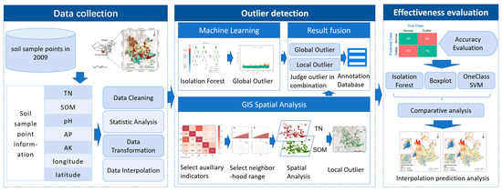
Figure 1.
Technology roadmap for the detection of TN outliers.
The proposed method is compared and analysed with the classical boxplot method and the OneClassSVM method. The boxplot method is a method that identifies global outliers based on quartiles and quartile distances [27]. The OneClassSVM method is an unsupervised algorithm based on a support vector machine to identify outliers [28]. This paper compares the detection performance of a single method (Isolation Forest, boxplot and OneClassSVM) and a combination of methods (the proposed method, the method that combines boxplot and local spatial autocorrelation, and the method that combines OneClassSVM and local spatial autocorrelation). The purpose of the combined method is to verify the effectiveness of local spatial autocorrelation analysis in identifying TN outliers by integrating both global and local anomalies.
2.1. Study Area
Yunnan Province is located on the southwestern border of China, with abundant agricultural resources, covering a total area of 394,100 square kilometres and extending from 21°8′–29°15′ N to 97°31′–106°11′ E. Due to its diverse climate and soil conditions, it is suitable for growing various crops, providing Yunnan Province with a rich variety of agricultural products and meeting the needs of different regions and markets. Among the agricultural resources in Yunnan Province, red soil is the most common soil type, accounting for 50% of the land area. Paddy soils are mainly found in basins and river valleys in central and eastern Yunnan Province, and most of them are neutral or slightly acidic. The organic matter content ranges from 1.5% to 3.0%, and the nitrogen and phosphorus nutrient content is higher than that of dryland soils. Dryland soils are mainly found in the mountain and plateau areas of western and northern Yunnan Province, covering about 64% of the province, and are mainly composed of red soil and loess. Dryland soils in the dam area account for about 17%, mainly composed of laterite. The distribution of dryland soils is relatively scattered, and the level of fertilisation is not high. In addition, soil erosion generally results in lower soil organic matter content compared to rice fields. In this study, 95 counties in Yunnan Province were selected as the study area, with a total of 25,930 observations. The scatterplot is shown in Figure 2.
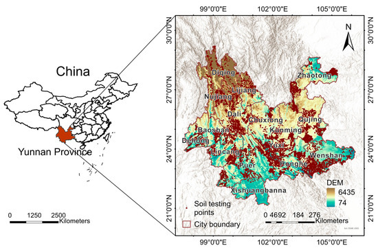
Figure 2.
Distribution map of soil test sites.
2.2. Correlation Analysis
We used Pearson’s correlation coefficient to measure the degree of linear correlation between two continuous variables. The formula for calculating Pearson’s correlation coefficient R is as follows:
where and are the characteristic variables; and are the means of data; the closer the value is to 1 or −1, the stronger the correlation; is a positive correlation, and is a negative correlation.
The Pearson’s correlation coefficient between TN and other soil nutrient indicators (e.g., pH, soil organic matter, available phosphorus, available potassium, etc.) was first calculated, and then the indicator with the strongest correlation with TN was selected as an auxiliary discriminator of local outliers. In the subsequent spatial analysis, TN and the auxiliary indicators were analysed separately, and the discriminant rule was applied to integrate the two results to determine the local outliers.
2.3. Isolation Forest
Isolation Forest (IForest) uses multiple isolated isolation trees (iTrees) to identify outliers in the data [29] and evaluates the degree of outlier by calculating the path length of the data point in the iTree. The shorter the path length, the higher the degree of outlier [30].
The process for identifying global outliers for TN is as follows: first, construct an iTree, randomly selecting a sub-sample from the TN dataset and selecting this sub-sample as the root node of the tree; then, randomly select a value from this sub-sample within the range of TN values as a partition value, dividing the data according to this partition value and thus creating a left and a right sub-tree, and repeat this step in the left and right sub-trees until the data are no longer divisible or until reaching the maximum height of the tree and the maximum depth of the tree, set to 20% of the total number of TN data points. The pseudocode of the iTree construction process is shown in Algorithm 1 (iTree building process).
| Algorithm 1: Building an itree |
| Input: |
| Output: an iTree |
| end if |
Secondly, 1000 iTrees are constructed to form IForest. The construction algorithm of IForest is shown in Algorithm 2 (IForest building process).
| Algorithm 2: iForest |
| Input: |
Finally, for each TN datum tested, traverse each iTree in the IForest, calculate the path length of each TN datum in each tree, calculate the outlier score of each TN datum based on the path length and determine whether each TN datum is an outlier or not, with the outlier ratio set to 0.05, and the outlier score calculation formula as follows:
where is the path length of sample from the root node to its leaf node, is the expected value of the path length in IForest and is the average value of for a given record . The formula is as follows:
where is the number of harmonic levels, which can be calculated as , and 0.5772156649 is Euler’s constant.
According to the anomaly score formula, if tends to 0, the anomaly score of the data is close to 1 and the data point is identified as anomalous; if tends to , the anomaly score is close to 0 and the data point is identified as normal; if the anomaly score tends to 0, it is not possible to determine whether the data is anomalous [27]. The IForest model in Sklearn modifies the anomaly scores so that a negative score indicates data outliers and a positive score indicates normal data.
2.4. Local Spatial Autocorrelation
Local spatial autocorrelation calculates the degree of similarity between units in a geospatial dataset and neighbouring units using Local Moran’s I [13]. For the local spatial autocorrelation analysis of TN data, if the Local Moran’s I is positive, it indicates that the TN data are similar to the surrounding neighbouring TN data, and there is the phenomenon of clustering of high–high (HH) or low–low (LL) values. Otherwise, the TN data are surrounded by the neighbouring TN data with different values, and the data is a distribution of high–low (HL) or low–high (LH) outliers. The expression for calculating the Local Moran’s I is given below:
where is the value of Local Moran’s I; is the measured value of a variable on spatial unit ; is the mean value of the variable; is the standardised value of the observed values of the attributes of spatial unit ; is the total number of observations of the variable, in units of one; and is the spatial weight between spatial units and .
To determine the weight matrix in Equation (4). The K-nearest-neighbours method is used, which is commonly used in the analysis of local spatial autocorrelation [31]. According to the official document of ArcGIS Pro, when the data are highly skewed, there should be no less than 8 neighbouring elements [32]. Therefore, we first set 5 K neighbouring points to construct a weight matrix and then gradually increased it to 30 neighbouring points to generate a spatial weight matrix under different K-value choices. Finally, the local spatial autocorrelation analysis of the data is carried out using different neighbouring elements to count the clustering results of the data under different K-values, and the change value of the spatial anomalous data from 5 to 30 is calculated. When the increment of the spatial anomalous data is the smallest, it is considered to be relatively stable, and the corresponding outlier is selected as a parameter to construct the weight matrix.
For the auxiliary indicators, K-values are selected in the same way, and local spatial autocorrelation analysis is performed based on the selected K-values to derive the distribution of HH/LL aggregates or HL/LH outliers. Based on the results of the spatial analysis, TN indicators and auxiliary indicators were combined to determine the spatial outliers. According to HL/LH abnormality, HH/LL aggregation and non-significance, the spatial outlier judgement can be divided into the following three types: (T1) if the TN detection result is HL/LH abnormality and the auxiliary indicator detection result is no abnormality or the abnormality result is inconsistent, it indicates that the datum is an outlier; (T2) if the TN shows clustering of HH or LL and the auxiliary indicator is opposite, the datum is an outlier; and (T3) if the TN shows insignificant results and the auxiliary indicator shows HL abnormality or LH abnormality, the datum is also an outlier.
2.5. Evaluation of Results
In model evaluation, the root mean square error, coefficient of determination, mean absolute error and Pearson’s correlation coefficient are commonly used to evaluate the quality of the proposed model [33,34]. However, in the binary classification problem, we are more concerned with the classification accuracy and misclassification of the model for different categories, so the observations can be classified into four categories based on the discrimination results and the actual situation: true positive (TP), false positive (FP), true negative (TN) and false negative (FN). Based on these four categories of observations, a second-order confusion matrix can be constructed (Table 1). In this case, the values on the main diagonal indicate the correct judgements made, and the values on the sub-diagonal indicate the incorrect judgements made. To effectively evaluate the performance of the proposed TN outlier identification method, six evaluation metrics are used: correct detection rate TR, false detection rate FR, true positive rate TPR, false positive rate FPR, true negative rate TNR and false negative rate FNR. These indices can reflect the discriminative ability and accuracy of the method for normal and abnormal observations. Among them, TR indicates the proportion of observations correctly classified as normal or abnormal out of the total observations. FR indicates the proportion of observations misclassified as normal or abnormal out of the total number of observations.

Table 1.
Confusion matrix of the second order.
Based on the second-order confusion matrix, the formula for the correct detection rate can be derived as follows:
The false positive rate is calculated using the following formula:
True positive rate:
False positive rate:
True negative rate:
False negative rate:
In the experiment, the expert discrimination results were taken as the actual results, and for the TN dataset, a combination of IForest and local spatial autocorrelation analysis was used to detect each data point, and the detection results were compared with the actual results to calculate the TR, FR, TPR, TNR, FPR and FNR.
2.6. Data Treatment with Computer Software
The training environment for the experiments was run on a high-performance computer configured with the following CPUs: Intel(R) Core(TM) i9-10980XE CPU @ 3.00 GHz, GPU: NVIDIA GeForce RTX 3090 and RAM: 64 GB. The IForest model was implemented using the Python language in the Sklearn library implemented in Python version 3.9.13. Data transformations were performed using STATA (17.0). All maps were generated using ArcGIS Pro (3.0.2) software, and other graphics were generated using Origin software (2022). Calculation of Local Moran’s I and spatial analysis were performed using ArcGIS Pro (3.0.2) software.
3. Results and Analysis
3.1. Analysis of Data Characteristics
This paper statistically analysed the soil test data of Yunnan Province in 2009 to explore the basic characteristics, distribution patterns and correlations of soil nutrient indicators. Five soil nutrient indicators were selected in this paper, namely total nitrogen (TN), pH, soil organic matter (SOM), available phosphorus (AP) and available potassium (AK). The raw datasets of these five indicators were analysed using basic mathematical statistics, and the results are presented in Table 2. The specific results are given below:
Table 2.
Basic statistical characteristics of soil nutrient data.
- (1)
- In terms of the mean value, according to the nutrient grading standard of the second national soil survey [35], the mean value of each nutrient content in Yunnan Province reached a high level, indicating that the soil nutrient status in Yunnan Province was generally good. Among them, the mean value of TN content was 1.78 g/kg, which was high; the mean value of pH was 6.20, which was slightly acidic; the mean value of SOM content was 33.70 g/kg, which was high; the mean value of AP content was 22.50 mg/kg, which was high; and the mean value of AK content was 148.50 mg/kg, which was relatively high.
- (2)
- In terms of the extreme values, the ratios of maximum to minimum values of TN, SOM, AP and AK were 2670 times, 1179 times, 5823 times and infinity, respectively, and the deviation of the maximum value from the mean value was far more than three times the range of the standard deviation, indicating that the range of values of soil nutrient data in Yunnan Province was large and there were obvious outliers. For example, the maximum value of TN was 26.70 g/kg, and the minimum value was 0.01 g/kg; the maximum value of SOM was 353.70 g/kg, and the minimum value was 0.30 g/kg; the maximum value of AP content was 582.30 mg/kg, and the minimum value was 0.10 mg/kg; and the maximum value of AK content was 19,940 mg/kg, and the minimum value was 0 mg/kg.
- (3)
- In terms of the coefficient of variation, pH had the lowest coefficient of variation of 16.13%, indicating that the degree of variation of pH was small; AP had the highest coefficient of variation of 108.44%, indicating that the degree of variation of AP was large; AK had the second-highest coefficient of variation of 83.10%; and the coefficients of variation of TN and SOM were both around 50%. These results reflect the heterogeneity and variability of soil nutrient data in Yunnan Province.
- (4)
- In terms of the normality test, the K-S test (p < 0.05) was used for analysis, and the results showed that TN, SOM, AP and AK in the original data did not follow normal distribution. After Box–Cox transformation, the data basically followed normal distribution.
In terms of correlation analysis, Figure 3 shows the Pearson’s correlation coefficients between TN and other indicators, all of which passed the significance test at the 0.05 level. The results showed that there was an overall positive correlation between TN and other indicators. Among them, the strongest correlation was between SOM and TN (R = 0.71), indicating a strong linear relationship between the two; the correlations between the rest of the indicators and TN were between 0.1 and 0.2, indicating a weak linear relationship between the two. Therefore, SOM was chosen as an auxiliary indicator for the local spatial autocorrelation analysis to determine whether the TN data were outliers. When TN is low, SOM is likely to be low, whereas when TN is high, SOM is likely to be high.
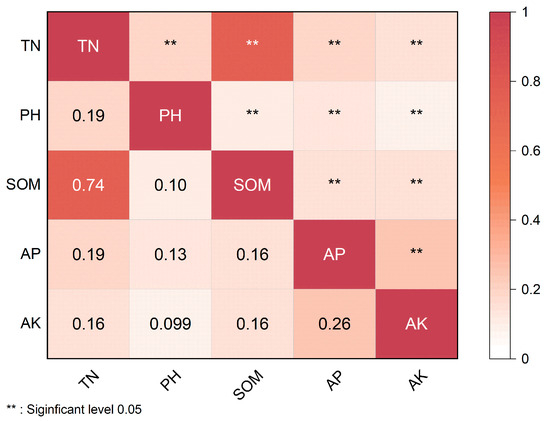
Figure 3.
Correlation between TN and remaining soil nutrients. Abbreviations: TN—total nitrogen, SOM—soil organic matter, AP—available phosphorus, AK—available potassium.
3.2. Hybrid Model Anomaly Identification Results
Based on the constructed model combining machine learning and spatial statistics to identify the TN data in Yunnan Province in 2009, both IForest and local spatial autocorrelation identified outliers, and the fusion of the two methods identified fewer outliers. As shown in Table 3, IForest identified 1291 outlier data points, local spatial autocorrelation identified 1519 outlier data points and the fusion method identified 59 anomalous data points. The outlier identification accuracies of the fusion method are as follows: where the correct detection rate (TR = 99.97%), false positive rate (FPR = 8.06%) and false negative rate (FNR = 0.01%) show high identification accuracies.
Table 3.
Results of the identification of outlier TN data in soils.
Figure 4 shows the distribution of the 59 TN outliers identified by the IForest and local spatial autocorrelation fusion methods on the map of Yunnan Province. According to Figure 4, the TN outliers are distributed in different regions of Yunnan Province, with the northwestern part of the country having a higher amount of outlier data, while the eastern part of the country has a lower amount of outlier data. This distribution may reflect the spatial heterogeneity of TN content and the influence of geological features. In addition, it is difficult to avoid the existence of some systematic errors or data anomalies caused by human factors in large-scale regional surveys. These outliers do not exist objectively but are often caused by random errors in sampling, experimental procedures, data processing, etc. Random errors cause outliers to be randomly distributed in the dataset, and the TN outliers distributed in different parts of Yunnan Province reflect the presence of such random outliers.
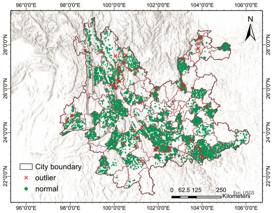
Figure 4.
Distribution of soil TN outliers identified by the fusion method.
Table 4 shows the types of spatial anomalies of TN outliers detected by the model. Among them, the main categories T1–T3 correspond to one to three discriminatory results of the discriminatory rule described in Section 2.4.
Table 4.
Types of spatial anomalies in TN.
- (1)
- There were 18 data points where TN anomalies and SOM anomalies are not consistent, indicating that there is no positive correlation between them. Of these 18 data points, 11 are HL anomalies where the TN content is high and the SOM content is low compared to other nearby points, and 7 are LH anomalies where the TN content is low compared to other nearby points and the SOM content is high compared to other nearby points. These data points may have measurement errors or other confounding factors.
- (2)
- There were 31 data points where the aggregation patterns of TN and SOM were completely opposite, indicating a negative correlation between them. Of these 31 data points, 6 data points have TN clustered as HH but SOM clustered as LL; 25 data points have TN clustered as LL and SOM clustered as HH. These data points may represent specific soil types or geographical conditions.
- (3)
- There were 10 data points where TN shows insignificant results and the SOM shows HL/LH abnormality, indicating that there was no significant linear relationship between the two. Of these 10 data points, 4 data points are HL anomalies, indicating that the SOM values of these data points are high compared to other points in the vicinity, and 6 data points are LH anomalies, indicating that the SOM values of these data points are low compared to other points in the vicinity. These data points may have other confounding factors or random variation.
3.3. Analysis of Contributions within the Hybrid Model
To further clarify the contribution of different models to the hybrid model, Figure 5 shows the distribution of global outliers partially identified by the IForest algorithm in the Yunnan TN dataset, with a total of 25,930 pieces of detected data and 1291 pieces of outliers, accounting for 4.98% of the total data volume. Figure 5 shows that the outliers identified by IForest are mostly concentrated in [0 g/kg, 0.5 g/kg] and [3.9 g/kg, +∞]. Among them, all values above 4.2 g/kg were judged as outliers, and about 47.25% and 11.46% of the values between 0–0.5 g/kg and 3.9–4.2 g/kg were judged as outliers.
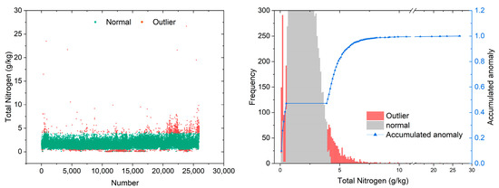
Figure 5.
Results of identification of global anomalies of TN in soil.
In addition, the study used the K-nearest-neighbours method to construct a spatial weight matrix for local spatial autocorrelation analysis. By calculating the number of local anomalies of TN and SOM under different numbers of neighbours, the spatial distribution and anomaly characteristics of these variables are understood. The combination of IForest and local spatial autocorrelation analysis provides outlier detection and spatial analysis at both global and local levels, leading to a more comprehensive understanding of the changing patterns of TN data. As illustrated in Figure 6, when the number of neighbours is 20, the spatial anomaly data of TN has the least amount of change, with only four data points changing from normal to abnormal or from abnormal to normal. This indicates that when the number of neighbours is 20, the distribution state of the spatial anomaly data of TN is relatively stable and not easily affected by the number of neighbours. When the number of neighbours is 25, the amount of change in the spatial anomaly data of SOM is the smallest, with only 29 data points changing from normal to abnormal or from abnormal to normal. This indicates that when the number of neighbours is 25, the spatial anomaly data distribution state of SOM is relatively stable and not easily affected by the number of neighbours. Therefore, the number of neighbours is chosen as 20 and 25 to perform the local spatial autocorrelation analysis for TN and SOM, respectively.
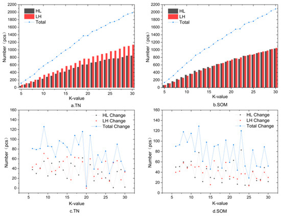
Figure 6.
The number of outliers in soil nutrient content for different values of K. The bar graphs show the number of spatial anomaly data for TN (a) and SOM (b), and the blue line graphs show the sum of HL and LH anomalies; (c,d) are line graphs showing the number of outliers in TN and SOM as a function of the number of neighbours K. Abbreviations: TN—total nitrogen, SOM—soil organic matter.
Based on the relatively stable K-neighbourhood values, local spatial autocorrelation analysis was performed using K = 20 for TN and K = 25 for SOM. As shown in Figure 7a, the results of HH and LL clustering of TN and the distribution of HL and LH spatial outliers derived from local spatial autocorrelation analyses at K = 20, and the results of spatial clustering and outlier distribution for SOM are shown in Figure 7b. The TN clustering and SOM clustering in Yunnan Province are basically the same and show a strong correlation. The distribution of HL outliers and LH outliers is also basically the same, with HL outliers mainly distributed near the LL clusters and LH outliers mainly distributed near the HH clusters (Figure 7).
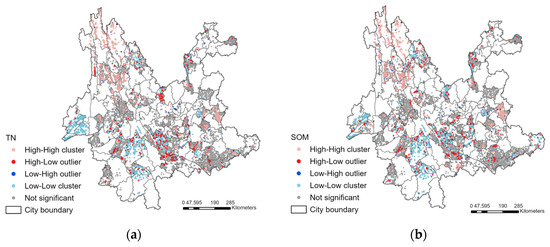
Figure 7.
Results of local spatial autocorrelation analyses of TN (a) and SOM (b). Abbreviations: TN—total nitrogen, SOM—soil organic matter.
A total of 25,930 data were detected by local spatial autocorrelation analysis, and the specific results are shown in Table 5. Among them, 15,337 data of TN are not significant, and 3545 data of HH clustering, 5669 data of LL clustering, 613 data of HL anomaly and 766 data of LH anomaly were detected. A total of 13,683 data of SOM are not significant, and 4018 data of HH clustering, 6467 data of LL clustering, 871 data of HL anomaly and 891 data of LH anomaly were detected.
Table 5.
Results of the identification of spatial anomalies in TN and SOM.
Figure 8 shows the results of the spatial outlier fusion of SOM as an auxiliary indicator to judge TN. According to the spatial outlier judging method described in Section 2.4, a total of 1519 spatial outliers were identified. Among them, 737 data were TN and SOM anomaly type inconsistency, 86 were TN and SOM aggregation mode completely opposite, 696 were TN manifestation of not significant and soil organic matter was HL/LH anomaly. In the geographical distribution of the TN spatial anomaly data, the TN spatial outliers were distributed in all sampling areas of Yunnan Province, reflecting a strong randomness.
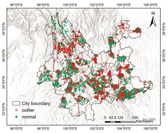
Figure 8.
Distribution of spatial anomalies of TN.
3.4. Comparison of Anomaly Detection Accuracy of Different Models
Figure 9 shows the distribution of the global outlier detection results using boxplots and OneClassSVM. The outliers detected by boxplot and OneClassSVM are mainly distributed in the head and tail, which is consistent with the distribution pattern of global outlier detection. The boxplots detect 1030 high-value outliers when detecting the original data, but no low-value outliers. This may be due to the fact that the raw data have a right-skewed, long-tailed distribution, which makes it easier to identify high-value outliers. To remedy this, this paper performs a Box–Cox transformation on the original data to make it closer to a normal distribution. The transformed boxplot was used to identify 1064 outliers, covering both high- and low-value outliers. In addition, OneClassSVM is not affected by the right-skewed distribution of the data when identifying data anomalies. OneClassSVM identifies a total of 1293 outliers.
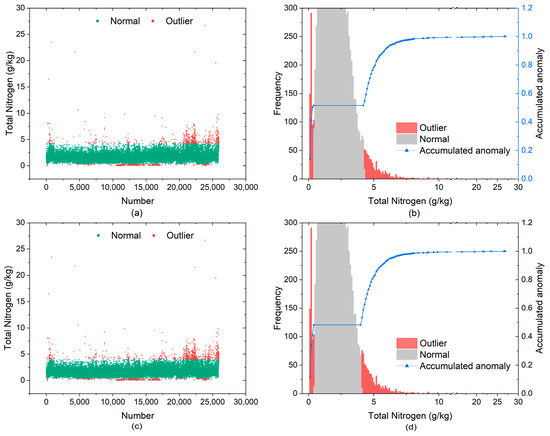
Figure 9.
Distribution of identification results for TN by boxplot (a,b), OneClassSVM (c,d).
Figure 9a shows the distribution of global outliers identified by the boxplot method in the TN dataset of Yunnan Province, with a total of 25,930 pieces of detected data and 1064 pieces of outlier data, accounting for 4.10% of the total data volume. Figure 9b shows that the outliers identified using the boxplot are mainly concentrated in [−∞, 0.4 g/kg] and [4.2 g/kg, +∞]. Among them, all values below 0.3 g/kg and above 4.3 g/kg were considered outliers. Figure 9c shows the distribution of global outliers identified by the OneClassSVM method in the TN dataset of Yunnan Province, with a total of 25,930 detected data and 1293 outliers, accounting for 4.99% of the total data volume. With respect to Figure 9d, the outliers detected by the OneClassSVM are mainly concentrated in [−∞, 0.4 g/kg] and [4.0 g/kg, +∞]. Among them, all values below 0.3 g/kg and above 4.2 g/kg are considered outliers. Approximately 6.96% and 5.03% of the data between 0.3–0.4 g/kg and 4.0–4.1 g/kg, respectively, are judged as outliers.
According to the effect analysis (Table 6), the higher the TR, TPR and TNR, the better, while the lower the FR, FPR and FNR, the better. Table 6 shows that the correct rate of all three methods is over 95%, but the false positive rate of the boxplot is higher at 11.29%.
Table 6.
Detection efficiency of IForest, boxplot and OneClassSVM methods.
Anomaly identification of TN data was performed using a combination of three methods, A, B and C. A is the proposed method (a combination of IForest and local spatial autocorrelation), B is a combination of boxplot and local spatial autocorrelation after Box–Cox transformation of the data and C is a combination of OneClassSVM and local spatial autocorrelation. When the original data were analysed using method B, a total of 35 outliers were identified, all of which were high-value outliers; when the transformed data were analysed, a total of 60 outliers were identified, with both high- and low-value outliers. There is a large change in the outlier identification results before and after transformation. The outliers identified by boxplot and local spatial autocorrelation analysis were classified, of which 15 were TN anomalous data inconsistent with the SOM anomaly type, 36 were TN aggregation mode completely opposite to the SOM aggregation mode and 9 were TN manifested as not significant, but SOM manifested as HL or LH anomalies. A total of 61 outliers were identified using method C, of which 16 were inconsistent between TN and SOM anomaly types, 35 were TN aggregated in a manner completely opposite to SOM aggregation, and 9 were TN behaving as not significant but SOM behaving as HL or LH anomalies. The detection performance using the combination of the three methods A, B and C is shown in Table 7. Regarding Table 7, it can be seen that the method proposed in this paper has the best detection performance with a TR of 99.97%, a TNR of 91.94%, an FPR of 8.06% and an FNR of 0.01%; the combination C method is the second best with a TR of 99.95%, a TNR of 88.89% and an FPR of 11.11%; and the combination B method has a correct detection rate of 99.94%, a TNR of 85.48%and FPR of 14.52%.
Table 7.
Legitimate detection effects for each group.
4. Discussion
To improve the accuracy of TN outlier identification, a TN outlier identification method combining IForest algorithm and local spatial autocorrelation analysis method is proposed in this study. The method is compared and evaluated with the traditional boxplot method and OneClassSVM unsupervised method. The 2009 soil test data of Yunnan Province was used as an example. The results show that the proposed method exhibits high effectiveness and accuracy in identifying TN outliers, with a TR as high as 99.97% and an FPR of 8.06%. In comparison, the correct detection rates of the traditional method were 96.08% and 95.23%, and the FPR was 11.29% and 6.45%, respectively. It can be seen that the new method has obvious advantages in identifying TN outliers, which not only improves accuracy but also avoids the occurrence of misclassification.
Comparison of the methods in this study with other methods shows that the combination methods are all superior to the individual methods in the detection of TN outliers. The combination of IForest, boxplot and OneClassSVM with local spatial autocorrelation all showed a significant improvement in detection, with all correct detection rates increasing by around 4%. This highlights the importance of combining global and local anomaly identification to significantly improve the accuracy of TN anomaly identification. This is because a single method can only assess anomalies from one perspective or dimension, whereas the combined method can combine multiple perspectives or dimensions, improving the completeness and accuracy of identification. IForest can quickly isolate global outliers but ignores the effect of spatial distribution; the boxplot can determine global outliers based on data distribution characteristics, but for skewed data, there are limitations in using the median to represent the overall assessment level, which may lead to data misclassification [36]. Meanwhile, OneClassSVM requires a longer training time [37]. Local spatial autocorrelation analysis methods can identify local outliers by evaluating the correlation between neighbouring observations in spatial data but may be affected by the choice of the spatial weight matrix. Combining these methods can compensate for the shortcomings of each method and exploit their respective strengths to achieve more effective and accurate identification of TN outliers. Compared to the other combination methods, method A showed the best performance in terms of detection accuracy with only 7 misclassified TN data, compared to 16 misclassified data in combination method B and 12 misclassified data in combination method C. The comparison of the correct detection rate, the true rate and the true negative rate of the identification results further confirmed the excellent results of the method.
Besides outliers, spatial autocorrelation analyses showed that TN in Yunnan Province showed an HH/LL aggregation pattern, mainly influenced by human activities, vegetation types and atmospheric deposition [38]. The results of local spatial autocorrelation analyses of TN in Yunnan Province showed that TN was higher in the northwestern plateau region and lower in the southwestern region, which was consistent with the findings of Zhang et al. [39]. The main reason for the higher soil TN content in the Northwest Plateau region is that the low temperature at high altitudes reduces or inhibits the activities of microorganisms involved in decomposition of soil organic matter [40]. In contrast, the soil types in the southwestern region are predominantly red soils and highly soluble lateritic soils with low nutrient content [41]. Low-nutrient soils with flat terrain, which are the main basis for agricultural production, are found in the central and southeastern regions [41]. The application of N fertiliser in agricultural production activities can provide sufficient source of N and thus increase the level of soil productivity [42]. It can be seen that the TN content in Yunnan Province is not only influenced by natural factors such as topography, geology and climate but also by anthropogenic factors such as agricultural activities. By analysing the outliers and spatial distribution pattern of TN, it can provide scientific basis and reference suggestions for soil nutrient management and agricultural production guidance in Yunnan Province.
To observe the change in spatial variability after removing the anomalies, Figure 10 shows a map of TN predicted for Yunnan Province using the inverse distance weighting method. The inverse distance weighting method is a spatial interpolation method that estimates the value of an unknown point based on a weighted average of the value of the known point and the inverse of the distance. The data used in Figure 10a are the original data, and Figure 10b shows the dataset after the anomalies have been removed using the proposed method. The coefficient of variation decreases from 53.37% to 51.02% after removing the outliers, indicating a more uniform distribution of the data. Meanwhile, parameters such as nuggets and sills can be calculated from the semi-variogram. Nugget refers to the value of the semi-variogram when the distance between two points is zero, reflecting randomness or measurement error in the data. Sill refers to the stable value reached by the semi-variogram when the distance between two points is large enough to reflect all the variability in the data. The nugget-to-sill ratio reflects the strength of spatial autocorrelation [43]. The nugget-to-sill ratio decreased from 54.17% to 53.95%, indicating an increase in spatial autocorrelation, suggesting that the total nitrogen content of soils in similar locations is more similar. The results of the TN prediction study can be used for soil nutrient analysis to provide guidance for agricultural production management.
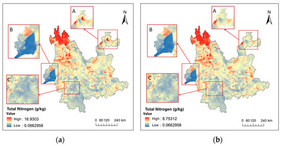
Figure 10.
Predicted distribution of TN in Yunnan Province. (a) Before removing outliers. (b) After removing outliers. A, B and C are one-to-one correspondence.
5. Conclusions
For the problem of detecting anomalies in TN data, we proposed a method for identifying TN outliers by combining the isolated forest algorithm and the local spatial autocorrelation analysis method and identified the outliers of TN data in Yunnan Province in 2009 and reached the following conclusions: (1) The overall situation of TN content in Yunnan Province is good, and at the same time, TN is positively correlated with SOM, PH, AP and AK relationship, and had a strong correlation with soil organic matter (R = 0.74). (2) The proposed method has high detection validity and accuracy in detecting TN anomalies, and in the detection effect of 2009 TN data in Yunnan Province, it showed that the TR could reach 99.97%, and the FNR was 0.01%. (3) Comparing the proposed method with the independent isolated forest (FNR = 4.76%), boxplot (FNR = 3.90%), OneClassSVM (FNR = 4.77%) and the combination method of boxplot, OneClassSVM combined with spatial analysis, respectively, the results show that the proposed method (FNR = 0.01%) is better than the single method and other combination methods. (4) The spatial distribution of TN content in Yunnan Province showed a trend of high in the northwest and low in the southwest, with the high-value area mainly distributed in northwest Yunnan and the low-value area mainly concentrated in southwest Yunnan. The fusion method of isolated forest and local spatial autocorrelation analysis can be used to effectively identify outliers in the analytical processing of soil total nitrogen data, thereby improving data quality. After outlier removal, the variability of the data is reduced, and the spatial autocorrelation is enhanced.
The method has the following advantages and innovations: (1) The method fully considers the spatial characteristics of TN data and improves the accuracy and comprehensiveness of outlier identification. (2) The IForest algorithm, as a global outlier detection tool, is capable of handling complex data with high speed and accuracy [44]. (3) Local spatial autocorrelation as a local outlier detection tool is capable of detecting spatial anomalies [45]. (4) The method integrates the discriminative results of global and local outliers for the final classification of the data, which avoids the possible misjudgement or omission of a single method and improves the reliability and stability of outlier identification. This study provides a new idea and method for the identification of TN outliers and supports soil nutrient analysis and evaluation, as well as the mining of soil fertility models.
Although the proposed methods show better results in identifying TN outliers, both the IForest algorithm and the local spatial autocorrelation analysis include some parameter settings, and the anomaly detection results are affected by the parameter settings, which may lead to unstable or inconsistent detection results. We can consider using some outlier detection methods based on integrated learning or deep learning to improve the stability and consistency of the detection results in future work. The stability and consistency of the detection results, as well as the use of some spatial outlier detection methods based on multiple indicators or multiple scales, can improve the accuracy and sensitivity of the detection results.
Author Contributions
Methodology, R.L., J.Y. and W.Z.; investigation, L.Y. and L.G.; validation, W.Z., R.L., J.Y. and L.Z.; formal analysis, R.L.; resources, L.Y.; data curation, L.Y. and L.G.; writing—original draft preparation, R.L.; writing—review and editing, J.Y.; visualisation, R.L.; supervision, L.G., J.Y. and L.Z.; project administration, J.Y.; funding acquisition, L.Z. All authors have read and agreed to the published version of the manuscript.
Funding
This work was supported by the National Key R&D Program of China (2022YFD1900803), the Yunnan Provincial Major Science and Technology Special Project (202202AE090013) and Beijing Academy of Agriculture and Forestry Sciences Major Scientific and Technological Achievement Cultivation Project: Key Technology Equipment and Industrialization of Smart Irrigation.
Institutional Review Board Statement
Not applicable.
Informed Consent Statement
Not applicable.
Data Availability Statement
Not applicable.
Conflicts of Interest
The authors declare no conflict of interest.
References
- Liu, H.; Zhu, Q.; Xia, X.; Li, M.; Huang, D. Multi-Feature Optimization Study of Soil Total Nitrogen Content Detection Based on Thermal Cracking and Artificial Olfactory System. Agriculture 2022, 12, 37. [Google Scholar] [CrossRef]
- Song, X.; Gao, Y.; Liu, Z.; Zhang, M.; Wan, Y.; Yu, X.; Liu, W.; Li, L. Development of a Predictive Tool for Rapid Assessment of Soil Total Nitrogen in Wheat-Corn Double Cropping System with Hyperspectral Data. Environ. Pollut. Bioavailab. 2019, 31, 272–281. [Google Scholar] [CrossRef]
- Ma, J.; Cheng, J.; Wang, J.; Pan, R.; He, F.; Yan, L.; Xiao, J. Rapid Detection of Total Nitrogen Content in Soil Based on Hyperspectral Technology. Inf. Process. Agric. 2022, 9, 566–574. [Google Scholar] [CrossRef]
- Nelson, D.W.; Sommers, L.E. Total Nitrogen Analysis of Soil and Plant Tissues. J. Assoc. Off. Anal. Chem. 1980, 63, 770–778. [Google Scholar] [CrossRef]
- Ren, K.; Xu, M.; Li, R.; Zheng, L.; Liu, S.; Reis, S.; Wang, H.; Lu, C.; Zhang, W.; Gao, H.; et al. Optimizing Nitrogen Fertilizer Use for More Grain and Less Pollution. J. Clean. Prod. 2022, 360, 132180. [Google Scholar] [CrossRef]
- Wang, H.; Bah, M.J.; Hammad, M. Progress in Outlier Detection Techniques: A Survey. IEEE Access 2019, 7, 107964–108000. [Google Scholar] [CrossRef]
- Pusch, M.; Samuel-Rosa, A.; Oliveira, A.L.G.; Magalhães, P.S.G.; Do Amaral, L.R. Improving Soil Property Maps for Precision Agriculture in the Presence of Outliers Using Covariates. Precis. Agric. 2022, 23, 1575–1603. [Google Scholar] [CrossRef]
- Fu, W.; Zhao, K.; Zhang, C.; Wu, J.; Tunney, H. Outlier Identification of Soil Phosphorus and Its Implication for Spatial Structure Modeling. Precis. Agric. 2016, 17, 121–135. [Google Scholar] [CrossRef]
- Zhang, C.; Selinus, O. Statistics and GIS in Environmental Geochemistry—Some Problems and Solutions. J. Geochem. Explor. 1998, 64, 339–354. [Google Scholar] [CrossRef]
- Chen, H.; Lu, X.; Gao, T.; Chang, Y. Identifying Hot-Spots of Metal Contamination in Campus Dust of Xi’an, China. Int. J. Environ. Res. Public. Health 2016, 13, 555. [Google Scholar] [CrossRef]
- Zhang, C.; Tang, Y.; Luo, L.; Xu, W. Outlier Identification and Visualization for Pb Concentrations in Urban Soils and Its Implications for Identification of Potential Contaminated Land. Environ. Pollut. 2009, 157, 3083–3090. [Google Scholar] [CrossRef] [PubMed]
- Khan, I.U.; Vachal, K.; Ebrahimi, S.; Wadhwa, S.S. Hotspot Analysis of Single-Vehicle Lane Departure Crashes in North Dakota. IATSS Res. 2022, 47, 25–34. [Google Scholar] [CrossRef]
- Anselin, L. Local Indicators of Spatial Association—LISA. Geogr. Anal. 1995, 27, 93–115. [Google Scholar] [CrossRef]
- Zhang, C.; Luo, L.; Xu, W.; Ledwith, V. Use of Local Moran’s I and GIS to Identify Pollution Hotspots of Pb in Urban Soils of Galway, Ireland. Sci. Total Environ. 2008, 398, 212–221. [Google Scholar] [CrossRef]
- Yuan, Y.; Cave, M.; Zhang, C. Using Local Moran’s I to Identify Contamination Hotspots of Rare Earth Elements in Urban Soils of London. Appl. Geochem. 2018, 88, 167–178. [Google Scholar] [CrossRef]
- Wang, X.; Liu, E.; Yan, M.; Zheng, S.; Fan, Y.; Sun, Y.; Li, Z.; Xu, J. Contamination and Source Apportionment of Metals in Urban Road Dust (Jinan, China) Integrating the Enrichment Factor, Receptor Models (FA-NNC and PMF), Local Moran’s Index, Pb Isotopes and Source-Oriented Health Risk. Sci. Total Environ. 2023, 878, 163211. [Google Scholar] [CrossRef]
- Wang, F.-J.; Mei, C.-L.; Zhang, Z.; Xu, Q.-X. Testing for Local Spatial Association Based on Geographically Weighted Interpolation of Geostatistical Data with Application to PM2.5 Concentration Analysis. Sustainability 2022, 14, 14646. [Google Scholar] [CrossRef]
- Braei, M.; Wagner, S. Anomaly Detection in Univariate Time-Series: A Survey on the State-of-the-Art. arXiv 2020, arXiv:2004.00433. [Google Scholar]
- Debener, J.; Heinke, V.; Kriebel, J. Detecting Insurance Fraud Using Supervised and Unsupervised Machine Learning. J. Risk Insur. 2023, 90, 743–768. [Google Scholar] [CrossRef]
- Orlova, E.V. Methodology and Models for Individuals’ Creditworthiness Management Using Digital Footprint Data and Machine Learning Methods. Mathematics 2021, 9, 1820. [Google Scholar] [CrossRef]
- Orlova, E.V. Innovation in Company Labor Productivity Management: Data Science Methods Application. Appl. Syst. Innov. 2021, 4, 68. [Google Scholar] [CrossRef]
- Li, W.; Finsa, M.M.; Laskey, K.B.; Houser, P.; Douglas-Bate, R. Groundwater Level Prediction with Machine Learning to Support Sustainable Irrigation in Water Scarcity Regions. Water 2023, 15, 3473. [Google Scholar] [CrossRef]
- Li, S.; Zhang, K.; Duan, P.; Kang, X. Hyperspectral Anomaly Detection With Kernel Isolation Forest. IEEE Trans. Geosci. Remote Sens. 2020, 58, 319–329. [Google Scholar] [CrossRef]
- Gao, R.; Zhang, T.; Sun, S.; Liu, Z. Research and Improvement of Isolation Forest in Detection of Local Anomaly Points. J. Phys. Conf. Ser. 2019, 1237, 052023. [Google Scholar] [CrossRef]
- Rezaei, S.; Ranjineh Khojasteh, E.; Faridazad, M. Improving Geostatistical Predictions of Two Environmental Variables Using Bayesian Maximum Entropy in the Sungun Mining Site. Stoch. Environ. Res. Risk Assess. 2020, 34, 1775–1794. [Google Scholar] [CrossRef]
- Zhang, G.; Rui, X.; Fan, Y. Critical Review of Methods to Estimate PM2.5 Concentrations within Specified Research Region. ISPRS Int. J. Geo-Inf. 2018, 7, 368. [Google Scholar] [CrossRef]
- Zhao, C.; Yang, J. A Robust Skewed Boxplot for Detecting Outliers in Rainfall Observations in Real-Time Flood Forecasting. Adv. Meteorol. 2019, 2019, 1795673. [Google Scholar] [CrossRef]
- Zhu, S.; Li, C.; Fang, K.; Peng, Y.; Jiang, Y.; Zou, Y. An Optimized Algorithm for Dangerous Driving Behavior Identification Based on Unbalanced Data. Electronics 2022, 11, 1557. [Google Scholar] [CrossRef]
- Mensi, A.; Franzoni, A.; Tax, D.M.J.; Bicego, M. An Alternative Exploitation of Isolation Forests for Outlier Detection. In Proceedings of the Structural, Syntactic, and Statistical Pattern Recognition; Torsello, A., Rossi, L., Pelillo, M., Biggio, B., Robles-Kelly, A., Eds.; Springer International Publishing: Cham, Switzerland, 2021; pp. 34–44. [Google Scholar]
- Liu, F.T.; Ting, K.M.; Zhou, Z.-H. Isolation Forest. In Proceedings of the 2008 Eighth IEEE International Conference on Data Mining, Pisa, Italy, 15–19 December 2008; pp. 413–422. [Google Scholar]
- Gallo, J.L.; Ertur, C. Exploratory Spatial Data Analysis of the Distribution of Regional per Capita GDP in Europe, 1980–1995. Pap. Reg. Sci. 2003, 82, 175–201. [Google Scholar] [CrossRef]
- ArcGIS Pro. Available online: https://pro.ArcGIS.com (accessed on 14 June 2023).
- Singh, S.; Kasana, S.S. Quantitative Estimation of Soil Properties Using Hybrid Features and RNN Variants. Chemosphere 2022, 287, 131889. [Google Scholar] [CrossRef]
- Singh, S.; Kasana, S.S. Estimation of Soil Properties from the EU Spectral Library Using Long Short-Term Memory Networks. Geoderma Reg. 2019, 18, e00233. [Google Scholar] [CrossRef]
- Zhang, Z.; Jiao, J.; Chen, T.; Chen, Y.; Lin, H.; Xu, Q.; Cheng, Y.; Zhao, W. Soil Nutrient Evaluation of Alluvial Fan in the Middle and Lower Reaches of Lhasa River Basin. J. Plant Nutr. Fertitizer 2022, 28, 2082–2096. [Google Scholar]
- Hubert, M.; Vandervieren, E. An Adjusted Boxplot for Skewed Distributions. Comput. Stat. Data Anal. 2008, 52, 5186–5201. [Google Scholar] [CrossRef]
- Shahid, N.; Naqvi, I.H.; Qaisar, S.B. One-Class Support Vector Machines: Analysis of Outlier Detection for Wireless Sensor Networks in Harsh Environments. Artif. Intell. Rev. 2015, 43, 515–563. [Google Scholar] [CrossRef]
- Zhang, J.; Wang, Y.; Qu, M.; Chen, J.; Yang, L.; Huang, B.; Zhao, Y. Source Apportionment of Soil Nitrogen and Phosphorus Based on Robust Residual Kriging and Auxiliary Soil-Type Map in Jintan County, China. Ecol. Indic. 2020, 119, 106820. [Google Scholar] [CrossRef]
- Zhang, Y.; Ai, J.; Sun, Q.; Li, Z.; Hou, L.; Song, L.; Tang, G.; Li, L.; Shao, G. Soil Organic Carbon and Total Nitrogen Stocks as Affected by Vegetation Types and Altitude across the Mountainous Regions in the Yunnan Province, South-Western China. CATENA 2021, 196, 104872. [Google Scholar] [CrossRef]
- Zhang, Y.; Heal, K.V.; Shi, M.; Chen, W.; Zhou, C. Decreasing Molecular Diversity of Soil Dissolved Organic Matter Related to Microbial Community along an Alpine Elevation Gradient. Sci. Total Environ. 2022, 818, 151823. [Google Scholar] [CrossRef]
- Xingwu, D.; Li, R.; Guangli, Z.; Jinming, H.; Haiyan, F. Soil Productivity in the Yunnan Province: Spatial Distribution and Sustainable Utilization. Soil Tillage Res. 2015, 147, 10–19. [Google Scholar] [CrossRef]
- Hu, Q.; Liu, T.; Ding, H.; Li, C.; Tan, W.; Yu, M.; Liu, J.; Cao, C. Effects of Nitrogen Fertilizer on Soil Microbial Residues and Their Contribution to Soil Organic Carbon and Total Nitrogen in a Rice-Wheat System. Appl. Soil Ecol. 2023, 181, 104648. [Google Scholar] [CrossRef]
- Cambardella, C.A.; Moorman, T.B.; Novak, J.M.; Parkin, T.B.; Karlen, D.L.; Turco, R.F.; Konopka, A.E. Field-Scale Variability of Soil Properties in Central Iowa Soils. Soil Sci. Soc. Am. J. 1994, 58, 1501–1511. [Google Scholar] [CrossRef]
- Tan, X.; Yang, J.; Rahardja, S. Sparse Random Projection Isolation Forest for Outlier Detection. Pattern Recognit. Lett. 2022, 163, 65–73. [Google Scholar] [CrossRef]
- Li, W.; Dong, F.; Ji, Z. Research on Coordination Level and Influencing Factors Spatial Heterogeneity of China’s Urban CO2 Emissions. Sustain. Cities Soc. 2021, 75, 103323. [Google Scholar] [CrossRef]
Disclaimer/Publisher’s Note: The statements, opinions and data contained in all publications are solely those of the individual author(s) and contributor(s) and not of MDPI and/or the editor(s). MDPI and/or the editor(s) disclaim responsibility for any injury to people or property resulting from any ideas, methods, instructions or products referred to in the content. |
© 2023 by the authors. Licensee MDPI, Basel, Switzerland. This article is an open access article distributed under the terms and conditions of the Creative Commons Attribution (CC BY) license (https://creativecommons.org/licenses/by/4.0/).