
Dryland Winter Wheat Production and Its Relationship to Fine-Scale Soil Carbon Heterogeneity—A Case Study in the US Central High Plains

 ,
,  ,
,
Abstract
:1. Introduction
2. Materials and Methods
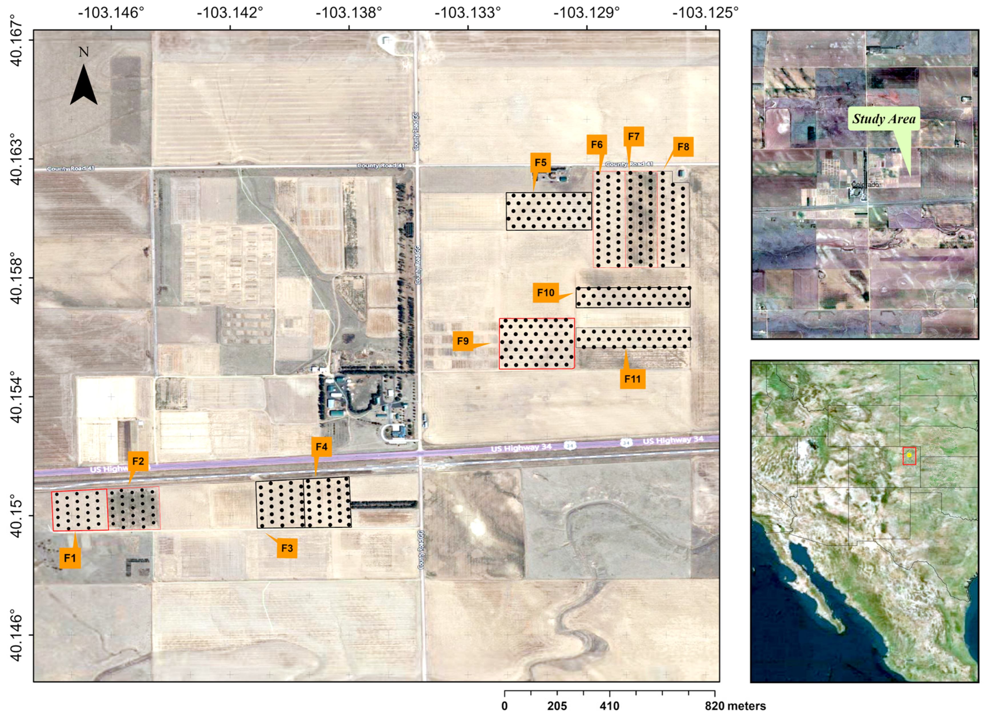
2.1. Study Site
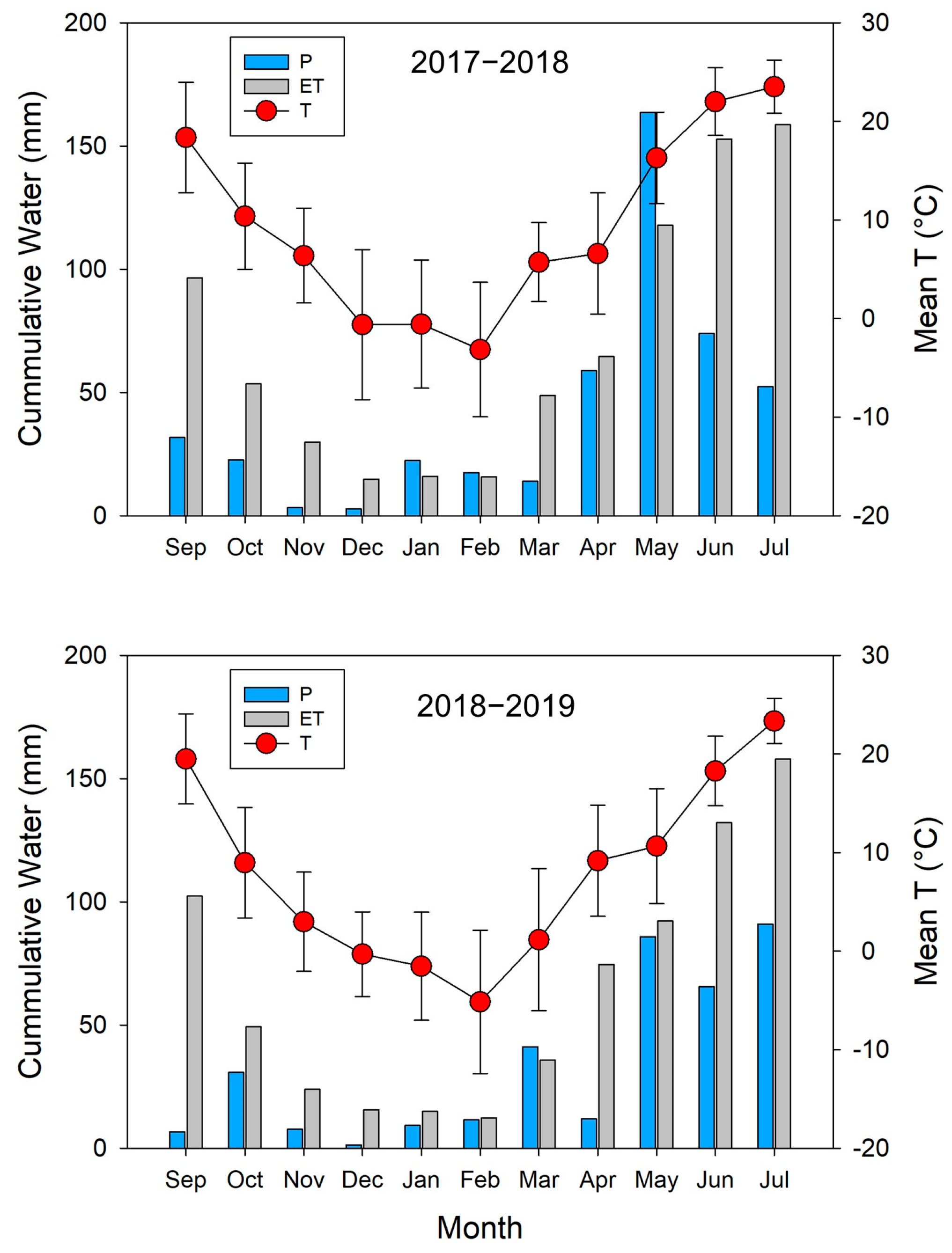
2.2. Climate Data
2.3. Experimental Design and Cropping Practices
2.4. Soil Sampling and Laboratory Analysis
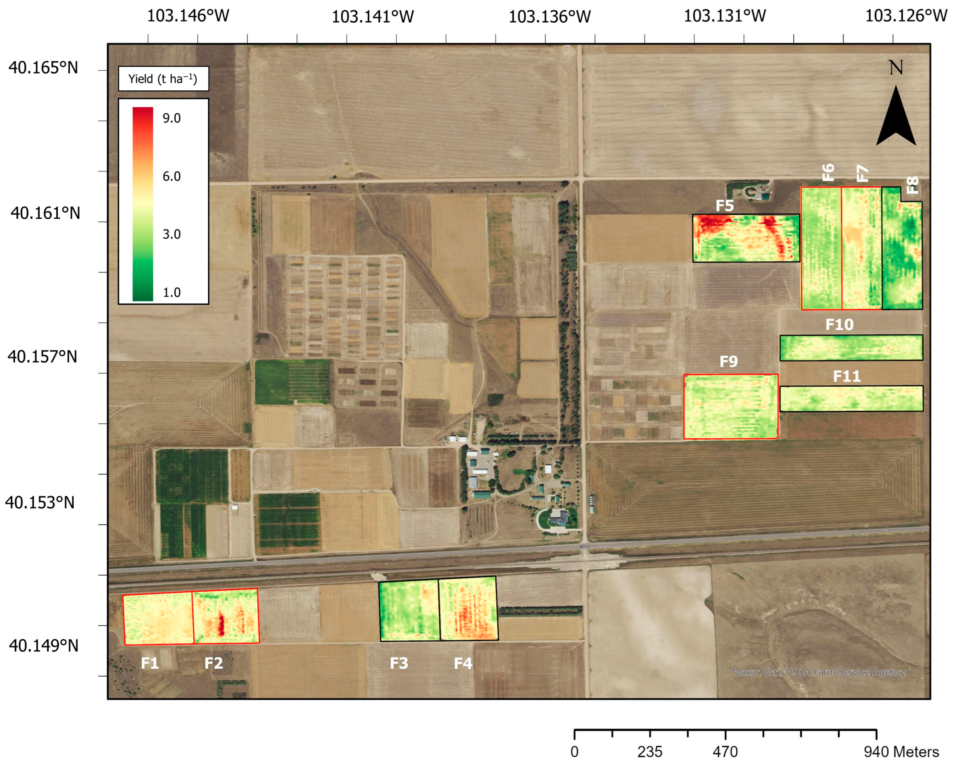
2.5. Processing of Yield Data and Mapping
2.6. Statistical Analysis
3. Results
3.1. Spatial Variability of Wheat Grain Yield
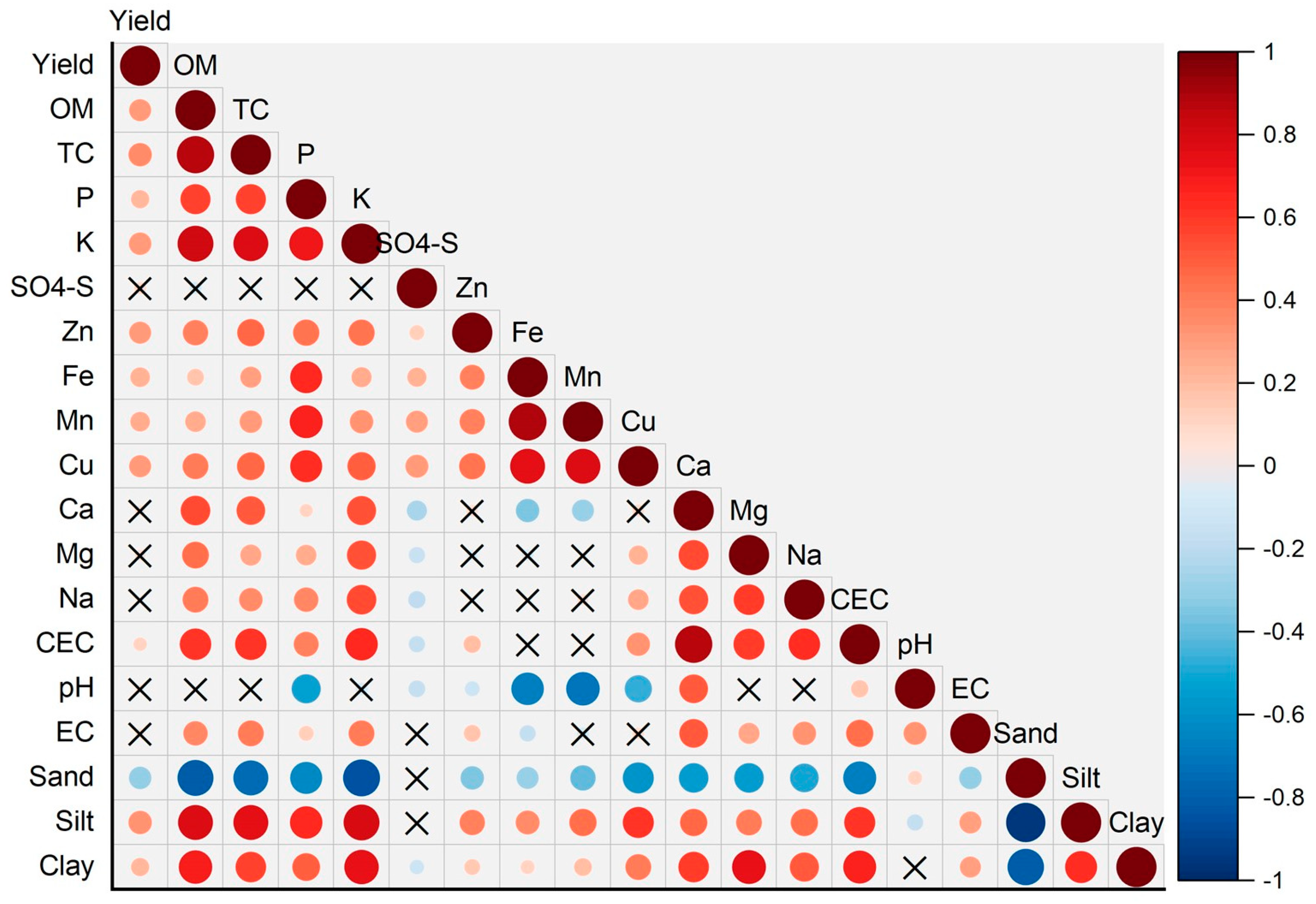
3.2. Relating Soil Attributes to Wheat Yield
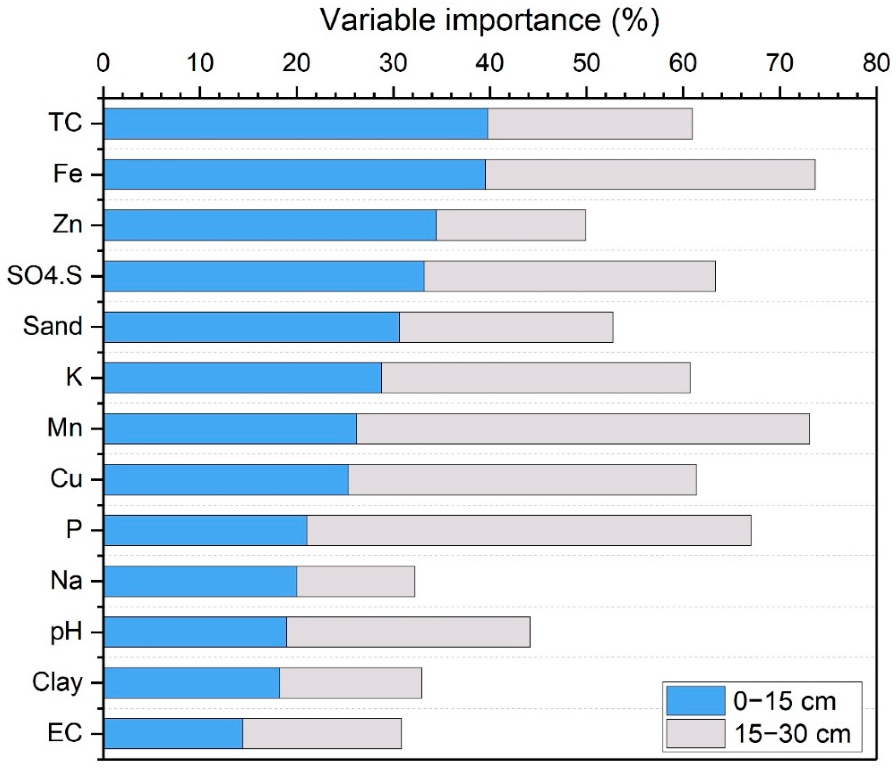
3.3. RF Variable Importance Analysis
4. Discussion
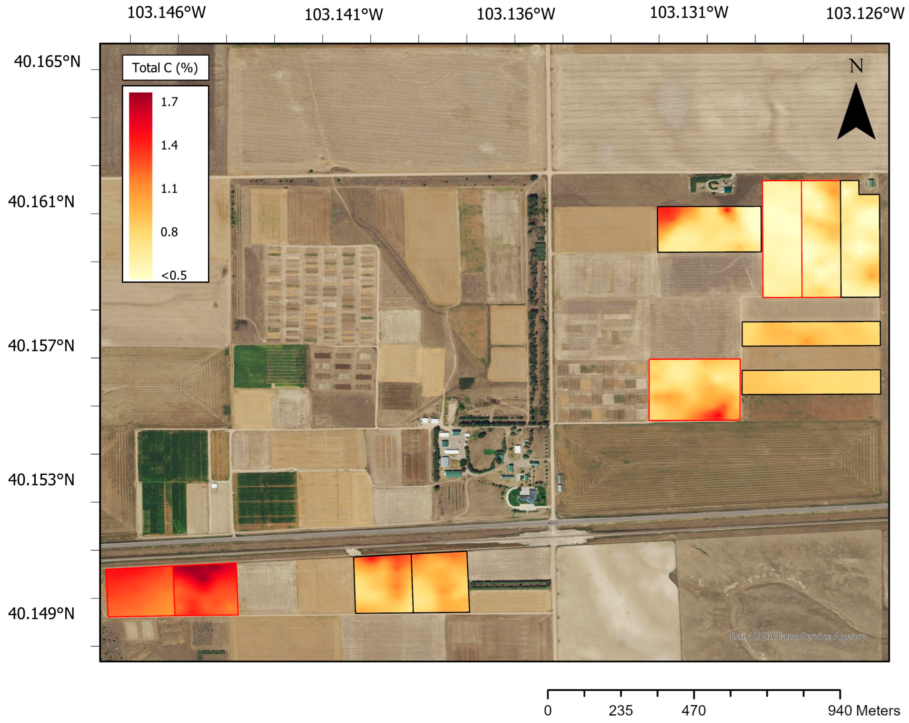
4.1. Spatial Distributions of Soil C and Wheat Grain Productivity
4.2. Relationship of Grain Yields to Nutrient Availability
4.3. Insights and Future Prospects
5. Conclusions
Supplementary Materials
Author Contributions
Funding
Data Availability Statement
Conflicts of Interest
References
- Ghimire, R.; Thapa, V.R.; Acosta-Martinez, V.; Schipanski, M.; Slaughter, L.C.; Fonte, S.J.; Shukla, M.K.; Bista, P.; Angadi, S.V.; Mikha, M.M.; et al. Soil Health Assessment and Management Framework for Water-Limited Environments: Examples from the Great Plains of the USA. Soil Syst. 2023, 7, 22. [Google Scholar] [CrossRef]
- Carr, P.M.; Bell, J.M.; Boss, D.L.; DeLaune, P.; Eberly, J.O.; Edwards, L.; Fryer, H.; Graham, C.; Holman, J.; Islam, M.A.; et al. Annual Forage Impacts on Dryland Wheat Farming in the Great Plains. Agron. J. 2021, 113, 1–25. [Google Scholar] [CrossRef]
- Rosenzweig, S.T.; Schipanski, M.E. Landscape-Scale Cropping Changes in the High Plains: Economic and Environmental Implications. Environ. Res. Lett. 2019, 14, 124088. [Google Scholar] [CrossRef]
- Ray, D.K.; Gerber, J.S.; MacDonald, G.K.; West, P.C. Climate Variation Explains a Third of Global Crop Yield Variability. Nat. Commun. 2015, 6, 5989. [Google Scholar] [CrossRef]
- Martinez-Feria, R.A.; Basso, B. Unstable Crop Yields Reveal Opportunities for Site-Specific Adaptations to Climate Variability. Sci. Rep. 2020, 10, 2885. [Google Scholar] [CrossRef]
- Usowicz, B.; Lipiec, J. Spatial Variability of Soil Properties and Cereal Yield in a Cultivated Field on Sandy Soil. Soil Tillage Res. 2017, 174, 241–250. [Google Scholar] [CrossRef]
- Lal, R. Soil Organic Matter Content and Crop Yield. J. Soil Water Conserv. 2020, 75, 27A–32A. [Google Scholar] [CrossRef]
- Oldfield, E.E.; Bradford, M.A.; Wood, S.A. Global Meta-Analysis of the Relationship between Soil Organic Matter and Crop Yields. Soil 2019, 5, 15–32. [Google Scholar] [CrossRef]
- Liang, S.; Li, L.; An, P.; Chen, S.; Shao, L.; Zhang, X. Spatial Soil Water and Nutrient Distribution Affecting the Water Productivity of Winter Wheat. Agric. Water Manag. 2021, 256, 107114. [Google Scholar] [CrossRef]
- Oelofse, M.; Markussen, B.; Knudsen, L.; Schelde, K.; Olesen, J.E.; Jensen, L.S.; Bruun, S. Do Soil Organic Carbon Levels Affect Potential Yields and Nitrogen Use Efficiency? An Analysis of Winter Wheat and Spring Barley Field Trials. Eur. J. Agron. 2015, 66, 62–73. [Google Scholar] [CrossRef]
- Hijbeek, R.; van Ittersum, M.K.; Berge, H.T.; Whitmore, A.P. Evidence Review Indicates a Re-Think on the Impact of Organic Inputs and Soil Organic Matter on Crop Yield. In Proceedings of the Proceedings-International Fertiliser Society 826, Cambridge, UK, 7 December 2018; pp. 1–28. [Google Scholar]
- Sale, P.W.; Gill, J.S.; Peries, R.R.; Tang, C. Crop Responses to Subsoil Manuring. I. Results in South-Western Victoria from 2009 to 2012. Crop Pasture Sci. 2018, 70, 44–54. [Google Scholar] [CrossRef]
- Gozdowski, D.; Leszczyńska, E.; Stępień, M.; Rozbicki, J.; Samborski, S. Within-Field Variability of Winter Wheat Yield and Grain Quality versus Soil Properties. Commun. Soil Sci. Plant Anal. 2017, 48, 1029–1041. [Google Scholar] [CrossRef]
- Taylor, J.C.; Wood, G.A.; Earl, R.; Godwin, R.J. Soil Factors and Their Influence on Within-Field Crop Variability, Part II: Spatial Analysis and Determination of Management Zones. Biosyst. Eng. 2003, 84, 441–453. [Google Scholar] [CrossRef]
- Agomoh, I.V.; Drury, C.F.; Phillips, L.A.; Reynolds, W.D.; Yang, X. Increasing Crop Diversity in Wheat Rotations Increases Yields but Decreases Soil Health. Soil Sci. Soc. Am. J. 2020, 84, 170–181. [Google Scholar] [CrossRef]
- Maestrini, B.; Basso, B. Drivers of Within-Field Spatial and Temporal Variability of Crop Yield across the US Midwest. Sci. Rep. 2018, 8, 14833. [Google Scholar] [CrossRef] [PubMed]
- Mulla, D.J.; Schepers, J.S. Key Processes and Properties for Site-Specific Soil and Crop Management. In The State of Site Specific Management for Agriculture; ASA, CSSA, and SSSA Books; American Society of Agronomy: Madison, WI, USA, 1997; pp. 1–18. [Google Scholar] [CrossRef]
- Jungkunst, H.F.; Göpel, J.; Horvath, T.; Ott, S.; Brunn, M. Global Soil Organic Carbon–Climate Interactions: Why Scales Matter. Wiley Interdiscip. Rev. Clim. Chang. 2022, 13, e780. [Google Scholar] [CrossRef]
- Zhu, M.; Feng, Q.; Qin, Y.; Cao, J.; Zhang, M.; Liu, W.; Deo, R.C.; Zhang, C.; Li, R.; Li, B. The Role of Topography in Shaping the Spatial Patterns of Soil Organic Carbon. CATENA 2019, 176, 296–305. [Google Scholar] [CrossRef]
- Peterson, F.S.; Lajtha, K.J. Linking Aboveground Net Primary Productivity to Soil Carbon and Dissolved Organic Carbon in Complex Terrain. J. Geophys. Res. Biogeosci. 2013, 118, 1225–1236. [Google Scholar] [CrossRef]
- Smidt, E.; Conley, S.; Zhu, J.; Arriaga, F.J. Identifying Field Attributes That Predict Soybean Yield Using Random Forest Analysis. Agron. J. 2016, 108, 637–646. [Google Scholar] [CrossRef]
- Whetton, R.L.; Zhao, Y.; Nawar, S.; Mouazen, A.M. Modelling the Influence of Soil Properties on Crop Yields Using a Non-Linear NFIR Model and Laboratory Data. Soil Syst. 2021, 5, 12. [Google Scholar] [CrossRef]
- Miner, G.L.; Delgado, J.A.; Ippolito, J.A.; Stewart, C.E. Soil Health Management Practices and Crop Productivity. Agric. Environ. Lett. 2020, 5, e20023. [Google Scholar] [CrossRef]
- Soil Survey Staff. Soil Taxonomy: A Basic System of Soil Classification for Making and Interpreting Soil Surveys, 2nd ed.; Agricultural Handbook 43; Natural Resources Conservation Service; United States Department of Agriculture: Washington, DC, USA, 1999.
- Olsen, S.R.; Sommers, L.E. Phosphorus. In Methods of Soil Analysis. Part 2: Chemical and Microbiological Properties; American Society of Agronomy: Madison, WI, USA, 1982; pp. 403–427. [Google Scholar]
- Soltanpour, P.N.; Schwab, A.P. A New Soil Test for Simultaneous Extraction of Macro- and Micro-nutrients in Alkaline Soils. Commun. Soil Sci. Plant Anal. 1977, 8, 195–207. [Google Scholar] [CrossRef]
- Soil Survey Staff. Kellogg Soil Survey Laboratory Methods Manual: Soil Survey Investigations Report No. 42, Version 5.0. R; Burt, R., Soil Survey Staff, Eds.; US Department of Agriculture, Natural Resources Conservation Service: Lincoln, NE, USA, 2014. [Google Scholar]
- Sudduth, K.A.; Drummond, S.T. Yield Editor: Software for Removing Errors from Crop Yield Maps. Agron. J. 2007, 99, 1471–1482. [Google Scholar] [CrossRef]
- Ganga, A.; Repe, B.; Elia, M.; Barrena-González, J.; Francisco, J.; Contador, L.; Pulido Fernández, M. Mapping Soil Properties at a Regional Scale: Assessing Deterministic vs. Geostatistical Interpolation Methods at Different Soil Depths. Sustainability 2022, 14, 10049. [Google Scholar] [CrossRef]
- Park, Y.; Li, B.; Li, Y. Crop Yield Prediction Using Bayesian Spatially Varying Coefficient Models with Functional Predictors. J. Am. Stat. Assoc. 2023, 118, 70–83. [Google Scholar] [CrossRef]
- Gribov, A.; Krivoruchko, K. Empirical Bayesian Kriging Implementation and Usage. Sci. Total Environ. 2020, 722, 137290. [Google Scholar] [CrossRef] [PubMed]
- Chabala, L.M.; Mulolwa, A.; Lungu, O. Application of Ordinary Kriging in Mapping Soil Organic Carbon in Zambia. Pedosphere 2017, 27, 338–343. [Google Scholar] [CrossRef]
- Krivoruchko, K.; Gribov, A. Evaluation of Empirical Bayesian Kriging. Spat. Stat. 2019, 32, 100368. [Google Scholar] [CrossRef]
- R Core Team. R: A Language and Environment for Statistical Computing; R Core Team: Vienna, Austria, 2021. [Google Scholar]
- Fox, J.; Weisberg, S. An R Companion to Applied Regression, 3rd ed.; Sage: Thousand Oaks, CA, USA, 2019. [Google Scholar]
- Paul, A.; Mukherjee, D.P.; Das, P.; Gangopadhyay, A.; Chintha, A.R.; Kundu, S. Improved Random Forest for Classification. IEEE Trans. Image Process. 2018, 27, 4012–4024. [Google Scholar] [CrossRef]
- Kuhn, M. Building Predictive Models in R Using the Caret Package. J. Stat. Softw. 2008, 28, 1–26. [Google Scholar] [CrossRef]
- Williams, A.; Hunter, M.C.; Kammerer, M.; Kane, D.A.; Jordan, N.R.; Mortensen, D.A.; Smith, R.G.; Snapp, S.; Davis, A.S. Soil Water Holding Capacity Mitigates Downside Risk and Volatility in US Rainfed Maize: Time to Invest in Soil Organic Matter? PLoS ONE 2016, 11, e0160974. [Google Scholar] [CrossRef]
- Lado, M.; Paz, A.; Ben-Hur, M. Organic Matter and Aggregate Size Interactions in Infiltration, Seal Formation, and Soil Loss. Soil Sci. Soc. Am. J. 2004, 68, 935–942. [Google Scholar] [CrossRef]
- Johnston, A.E.; Poulton, P.R.; Coleman, K. Chapter 1 Soil Organic Matter. Its Importance in Sustainable Agriculture and Carbon Dioxide Fluxes. Adv. Agron. 2009, 101, 1–57. [Google Scholar] [CrossRef]
- Augusto, L.; Achat, D.L.; Jonard, M.; Vidal, D.; Ringeval, B. Soil Parent Material-A Major Driver of Plant Nutrient Limitations in Terrestrial Ecosystems. Glob. Chang. Biol. 2017, 23, 3808–3824. [Google Scholar] [CrossRef] [PubMed]
- Miller, M.P.; Singer, M.J.; Nielsen, D.R. Spatial Variability of Wheat Yield and Soil Properties on Complex Hills. Soil Sci. Soc. Am. J. 1988, 52, 1133–1141. [Google Scholar] [CrossRef]
- Stewart, C.M.; Mcbratney, A.B.; Skerritt, J.H. Site-Specific Durum Wheat Quality and Its Relationship to Soil Properties in a Single Field in Northern New South Wales. Precis. Agric. 2002, 3, 155–168. [Google Scholar] [CrossRef]
- Zomer, R.J.; Bossio, D.A.; Sommer, R.; Verchot, L.V. Global Sequestration Potential of Increased Organic Carbon in Cropland Soils. Sci. Rep. 2017, 7, 15554. [Google Scholar] [CrossRef]
- Astolfi, S.; Celletti, S.; Vigani, G.; Mimmo, T.; Cesco, S. Interaction Between Sulfur and Iron in Plants. Front. Plant Sci. 2021, 12, 670308. [Google Scholar] [CrossRef]
- Kumar, D.; Patel, K.P.; Ramani, V.P.; Shukla, A.K.; Meena, R.S. Management of Micronutrients in Soil for the Nutritional Security. In Nutrient Dynamics for Sustainable Crop Production; Springer: Singapore, 2020; pp. 103–134. [Google Scholar]
- Carciochi, W.D.; Salvagiotti, F.; Pagani, A.; Reussi Calvo, N.I.; Eyherabide, M.; Sainz Rozas, H.R.; Ciampitti, I.A. Nitrogen and Sulfur Interaction on Nutrient Use Efficiencies and Diagnostic Tools in Maize. Eur. J. Agron. 2020, 116, 126045. [Google Scholar] [CrossRef]
- Zuo, Y.; Zhang, F. Soil and Crop Management Strategies to Prevent Iron Deficiency in Crops. Plant Soil 2011, 339, 83–95. [Google Scholar] [CrossRef]
- Tavakkoli, E.; Rengasamy, P.; McDonald, G.K. High Concentrations of Na+ and Cl− Ions in Soil Solution Have Simultaneous Detrimental Effects on Growth of Faba Bean under Salinity Stress. J. Exp. Bot. 2010, 61, 4449–4459. [Google Scholar] [CrossRef]
- Samui, R.C.; Bhattacharyya, P.; Dasgupta, S.K. Uptake of Nutrients by Mustard (Brassica Juncea L.) as Influenced by Zinc and Iron Application. J. Indian Soc. Soil Sci. 1981, 29, 101–106. [Google Scholar]
- Stadler, A.; Rudolph, S.; Kupisch, M.; Langensiepen, M.; van der Kruk, J.; Ewert, F. Quantifying the Effects of Soil Variability on Crop Growth Using Apparent Soil Electrical Conductivity Measurements. Eur. J. Agron. 2015, 64, 8–20. [Google Scholar] [CrossRef]
- Kitchen, N.R.; Drummond, S.T.; Lund, E.D.; Sudduth, K.A.; Buchleiter, G.W. Soil Electrical Conductivity and Topography Related to Yield for Three Contrasting Soil–Crop Systems. Agron. J. 2003, 95, 483–495. [Google Scholar] [CrossRef]
- Fenton, T.E.; Kazemi, M.; Lauterbach-Barrett, M.A. Erosional Impact on Organic Matter Content and Productivity of Selected Iowa Soils. Soil Tillage Res. 2005, 81, 163–171. [Google Scholar] [CrossRef]
- Williams, C.L.; Liebman, M.; Edwards, J.W.; James, D.E.; Singer, J.W.; Arritt, R.; Herzmann, D. Patterns of Regional Yield Stability in Association with Regional Environmental Characteristics. Crop Sci. 2008, 48, 1545–1559. [Google Scholar] [CrossRef]
- Kravchenko, A.N.; Robertson, G.P.; Thelen, K.D.; Harwood, R.R. Management, Topographical, and Weather Effects on Spatial Variability of Crop Grain Yields; Management, Topographical, and Weather Effects on Spatial Variability of Crop Grain Yields. Agron. J. 2005, 97, 514–523. [Google Scholar] [CrossRef]
- Schut, A.G.T.; Giller, K.E. Soil-Based, Field-Specific Fertilizer Recommendations Are a Pipe-Dream. Geoderma 2020, 380, 114680. [Google Scholar] [CrossRef]


| pH | EC | OM | TC | CEC | P | K | SO4-S | Zn | Fe | Mn | Cu | Ca | Mg | Na | Sand | Clay | Elev | |
|---|---|---|---|---|---|---|---|---|---|---|---|---|---|---|---|---|---|---|
| dS m−1 | wt % | wt % | cmol(+) kg−1 | mg kg−1 | mg kg−1 | mg kg−1 | mg kg−1 | mg kg−1 | mg kg−1 | mg kg−1 | mg kg−1 | mg kg−1 | mg kg−1 | % | % | m | ||
| Field 1 (n = 25) | ||||||||||||||||||
| Mean | 6.6 | 0.1 | 2.6 | 1.2 | 18.6 | 20.9 | 705 | 9.3 | 0.8 | 27.4 | 25.8 | 1.0 | 2553 | 378 | 8.0 | 32.6 | 28.0 | 1388 |
| SD | 0.5 | 0.1 | 0.4 | 0.1 | 3.6 | 7.5 | 61 | 1.6 | 0.5 | 9.8 | 10.5 | 0.2 | 740 | 63 | 1.4 | 4.2 | 2 | 1 |
| Field 2 (n = 27) | ||||||||||||||||||
| Mean | 6.5 | 0.2 | 2.7 | 1.4 | 21.3 | 31.8 | 766 | 10.9 | 0.7 | 28.2 | 30.9 | 1.0 | 2749 | 378 | 9.3 | 34.2 | 27.3 | 1387 |
| SD | 0.6 | 0.1 | 0.4 | 0.2 | 4.0 | 14.3 | 97 | 1.6 | 0.2 | 10.3 | 12.4 | 0.2 | 965 | 54 | 2.5 | 7.5 | 2.1 | 1 |
| Field 6 (n = 38) | ||||||||||||||||||
| Mean | 6.4 | 0.1 | 1.3 | 0.6 | 11.7 | 10.3 | 315 | 16.2 | 0.5 | 19.0 | 19.7 | 0.7 | 1478 | 280 | 6.1 | 63.6 | 19.8 | 1382 |
| SD | 0.4 | 0.1 | 0.2 | 0.1 | 3.1 | 4.8 | 78 | 3.0 | 0.4 | 11.0 | 7.5 | 0.2 | 558 | 87 | 1.8 | 6.1 | 3.2 | 1 |
| Field 7 (n = 38) | ||||||||||||||||||
| Mean | 6.4 | 0.1 | 1.6 | 0.7 | 11.5 | 13.1 | 366 | 15.4 | 0.6 | 21.8 | 23.7 | 0.8 | 1401 | 258 | 6.1 | 57.2 | 21.1 | 1382 |
| SD | 0.4 | 0 | 0.3 | 0.2 | 2.1 | 4.5 | 92 | 3.0 | 0.9 | 6.7 | 8.6 | 0.1 | 336 | 78 | 2.0 | 8.6 | 3.7 | 1 |
| Field 9 (n = 52) | ||||||||||||||||||
| Mean | 6.4 | 0.1 | 1.9 | 0.9 | 20.1 | 32.1 | 599 | 11.7 | 0.5 | 29.7 | 31.2 | 1.0 | 2487 | 343 | 10.1 | 41.3 | 25.4 | 1383 |
| SD | 0.8 | 0 | 0.3 | 0.2 | 4.1 | 13 | 107 | 8.8 | 0.1 | 14.4 | 15.9 | 0.2 | 1218 | 109 | 2.6 | 6.4 | 2.9 | 0 |
| pH | EC | OM | TC | CEC | P | K | SO4-S | Zn | Fe | Mn | Cu | Ca | Mg | Na | Sand | Clay | Elev | |
|---|---|---|---|---|---|---|---|---|---|---|---|---|---|---|---|---|---|---|
| dS m−1 | wt % | wt % | cmol(+) kg−1 | mg kg−1 | mg kg−1 | mg kg−1 | mg kg−1 | mg kg−1 | mg kg−1 | mg kg−1 | mg kg−1 | mg kg−1 | mg kg−1 | % | % | m | ||
| Field 3 (n = 30) | ||||||||||||||||||
| Mean | 5.9 | 0.1 | 2.3 | 0.9 | 16 | 33.6 | 746 | 7.3 | 0.5 | 22.8 | 27.3 | 0.8 | 1790 | 458 | 10.2 | 37.2 | 28.1 | 1387 |
| SD | 0.3 | 0 | 0.3 | 0.2 | 1.9 | 7.1 | 90 | 2.6 | 0.3 | 6.2 | 9.4 | 0.1 | 303 | 111 | 3.0 | 5.2 | 2.8 | 1 |
| Field 4 (n = 33) | ||||||||||||||||||
| Mean | 6.4 | 0.2 | 2.3 | 0.9 | 17.9 | 26.5 | 747 | 7.1 | 0.5 | 18.3 | 22.3 | 0.8 | 2237 | 521 | 13.3 | 36.2 | 29.3 | 1387 |
| SD | 0.5 | 0.1 | 0.2 | 0.1 | 4.9 | 6.2 | 77 | 1.6 | 0.2 | 5.6 | 6.5 | 0.1 | 843 | 139 | 7.5 | 4.0 | 3.0 | 1 |
| Field 5 (n = 42) | ||||||||||||||||||
| Mean | 6.3 | 0.1 | 1.8 | 0.8 | 12.8 | 23.2 | 475 | 6.0 | 0.5 | 39 | 26.3 | 0.7 | 1425 | 292 | 6.5 | 54.4 | 22.7 | 1381 |
| SD | 0.4 | 0 | 0.7 | 0.3 | 2.3 | 16.3 | 170 | 6.0 | 0.3 | 23.1 | 10.4 | 0.2 | 299 | 78 | 1.1 | 14.0 | 4.9 | 1 |
| Field 8 (n = 34) | ||||||||||||||||||
| Mean | 6.3 | 0.1 | 1.7 | 0.7 | 13.1 | 14.4 | 370 | 5.8 | 0.3 | 16.8 | 16.6 | 0.6 | 1711 | 293 | 7.8 | 57.7 | 21.1 | 1382 |
| SD | 0.7 | 0 | 0.3 | 0.1 | 5.0 | 5.2 | 66 | 1.5 | 0.2 | 7.9 | 7.9 | 0.1 | 905 | 116 | 2.8 | 8.3 | 3.7 | 1 |
| Field 10 (n = 35) | ||||||||||||||||||
| Mean | 6.3 | 0.1 | 2.0 | 0.8 | 14.9 | 26.4 | 549 | 9.7 | 0.6 | 25.9 | 23.5 | 0.8 | 1808 | 293 | 7.4 | 48.8 | 23.4 | 1383 |
| SD | 0.6 | 0.1 | 0.4 | 0.2 | 3.6 | 5.7 | 89 | 2.5 | 0.4 | 8.5 | 8.7 | 0.1 | 881 | 72 | 1.0 | 7.4 | 3.0 | 1 |
| Field 11 (n = 34) | ||||||||||||||||||
| Mean | 6.8 | 0.1 | 2.1 | 0.8 | 17.2 | 22.4 | 554 | 6.1 | 0.6 | 15 | 17.1 | 0.6 | 2254 | 430 | 7.7 | 46.3 | 27.0 | 1384 |
| SD | 0.6 | 0.1 | 0.3 | 0.2 | 2.9 | 9.5 | 75 | 3.7 | 0.7 | 8.8 | 9.9 | 0.1 | 769 | 112 | 0.9 | 8.0 | 3.2 | 0 |
Disclaimer/Publisher’s Note: The statements, opinions and data contained in all publications are solely those of the individual author(s) and contributor(s) and not of MDPI and/or the editor(s). MDPI and/or the editor(s) disclaim responsibility for any injury to people or property resulting from any ideas, methods, instructions or products referred to in the content. |
© 2023 by the authors. Licensee MDPI, Basel, Switzerland. This article is an open access article distributed under the terms and conditions of the Creative Commons Attribution (CC BY) license (https://creativecommons.org/licenses/by/4.0/).
Share and Cite
Ramírez, P.B.; Calderón, F.J.; Vigil, M.F.; Mankin, K.R.; Poss, D.; Fonte, S.J. Dryland Winter Wheat Production and Its Relationship to Fine-Scale Soil Carbon Heterogeneity—A Case Study in the US Central High Plains. Agronomy 2023, 13, 2600. https://doi.org/10.3390/agronomy13102600
Ramírez PB, Calderón FJ, Vigil MF, Mankin KR, Poss D, Fonte SJ. Dryland Winter Wheat Production and Its Relationship to Fine-Scale Soil Carbon Heterogeneity—A Case Study in the US Central High Plains. Agronomy. 2023; 13(10):2600. https://doi.org/10.3390/agronomy13102600
Chicago/Turabian StyleRamírez, Paulina B., Francisco J. Calderón, Merle F. Vigil, Kyle R. Mankin, David Poss, and Steven J. Fonte. 2023. "Dryland Winter Wheat Production and Its Relationship to Fine-Scale Soil Carbon Heterogeneity—A Case Study in the US Central High Plains" Agronomy 13, no. 10: 2600. https://doi.org/10.3390/agronomy13102600
APA StyleRamírez, P. B., Calderón, F. J., Vigil, M. F., Mankin, K. R., Poss, D., & Fonte, S. J. (2023). Dryland Winter Wheat Production and Its Relationship to Fine-Scale Soil Carbon Heterogeneity—A Case Study in the US Central High Plains. Agronomy, 13(10), 2600. https://doi.org/10.3390/agronomy13102600