Article

Choosing Feature Selection Methods for Spatial Modeling of Soil Fertility Properties at the Field Scale

by
Caner Ferhatoglu
and
Bradley A. Miller
*
Department of Agronomy, Iowa State University, Ames, IA 50011, USA
*
Author to whom correspondence should be addressed.
Agronomy 2022, 12(8), 1786; https://doi.org/10.3390/agronomy12081786
Submission received: 30 June 2022 / Revised: 22 July 2022 / Accepted: 25 July 2022 / Published: 29 July 2022

Abstract

:
With the growing availability of environmental covariates, feature selection (FS) is becoming an essential task for applying machine learning (ML) in digital soil mapping (DSM). In this study, the effectiveness of six types of FS methods from four categories (filter, wrapper, embedded, and hybrid) were compared. These FS algorithms chose relevant covariates from an exhaustive set of 1049 environmental covariates for predicting five soil fertility properties in ten fields, in combination with ten different ML algorithms. Resulting model performance was compared by three different metrics (R2 of 10-fold cross validation (CV), robustness ratio (RR; developed in this study), and independent validation with Lin’s concordance correlation coefficient (IV-CCC)). FS improved CV, RR, and IV-CCC compared to the models built without FS for most fields and soil properties. Wrapper (BorutaShap) and embedded (Lasso-FS, Random forest-FS) methods usually led to the optimal models. The filter-based ANOVA-FS method mostly led to overfit models, especially for fields with smaller sample quantities. Decision-tree based models were usually part of the optimal combination of FS and ML. Considering RR helped identify optimal combinations of FS and ML that can improve the performance of DSM compared to models produced from full covariate stacks.

1. Introduction

Digital soil mapping (DSM) has been widely used to map various soil properties and classes for the last few decades [1]. A strategy for DSM is the process of using predictive statistical models (e.g., machine learning (ML)) that utilize the relationships between georeferenced soil lab data and environmental predictors (aka covariates) [2]. Performance of ML relies heavily on the covariates used to represent true soil-landscape relationships. Therefore, covariate (aka feature) selection is an important aspect for this approach to DSM [3,4].
Growing availability of environmental covariates due to advancements in remote sensing (RS) technologies has made it challenging to select and focus on the most important covariates. Using only relevant covariates in modelling is crucial where the ‘curse of dimensionality’ can negatively impact the bias-variance tradeoff in modelling with small datasets, for example, the datasets commonly used in field-scale soil mapping [5,6], plant-breeding studies [7], classification of microshoots and somatic embryos for in vitro culture [8], and stress phenotyping [9]. The ’curse of dimensionality’ refers to the modelling problem that the growth in dimensions—each covariate is a dimension—in the feature space requires an exponentially increasing number of training samples for a ML algorithm to avoid over-fitting and build reliable models [10]. However, gathering all available potential environmental covariates is beneficial for not missing any spatial information that could be useful for predictions. In this context, feature selection (FS) algorithms help reduce dimensionality stemming from a large covariate stack by identifying covariates that are most likely to be relevant.
Objectives of FS, as a data pre-processing strategy, include building more comprehensible and simpler models, reducing computational requirements, reducing the effect of the curse-of-dimensionality, and improving prediction performance [11,12]. FS strategies can be grouped as filter, wrapper, embedded, and hybrid [13]. The most popular FS methods in the DSM studies are filter and wrapper strategies [14]. Filter strategies perform FS based on characteristics of data to evaluate the usefulness of covariates [15]. For example, a filter FS strategy based on correlation between covariates eliminates redundant covariates by reducing highly correlated covariates. For the most part, these methods are computationally efficient [12]. However, because there is no learning algorithm guiding the selection process, the selected covariates may not be the optimal selection for specific ML algorithms.
Wrapper strategies use a ML algorithm as a learning object and iteratively add or remove covariates from a covariate pool to find the optimal combination of covariates for maximizing model performance [16]. The most commonly used wrapper strategy in DSM studies is recursive feature elimination (RFE) [14]. Wrapper strategies are often called ‘greedy’ search algorithms due to the extensive search space during the selection. Thus, they typically require longer computation times relative to the other FS strategies [17]. Despite that, wrapper strategies can be advantageous in identifying non-linear complex relationships between the target soil property and covariates.
In addition to popular wrappers, new wrapper algorithms have been emerging. However, these newer wrapper algorithms have not been tested in the context of DSM. For example, BorutaShap-FS [18] has been found useful in many applications such as COVID-19 severity prediction [19] and predicting the height of buildings from Sentinel-1 and -2 data [20]. BorutaShap-FS combines the Boruta algorithm [21] with SHAP (SHapley Additive exPlanations) [22], which is a game theoretic approach to explain the output of a ML model. The Boruta algorithm first generates five shadow covariates whose values are obtained by shuffling values of the original covariate to remove their correlations with the target variable (soil properties). Then, Shapley values [23] are computed to determine the importance of covariates and their shadow covariates. SHAP calculates covariate importance based on calculating how much each covariate contributes to the model. In BorutaShap-FS, covariates whose SHAP importance score is higher than the shadow covariates are selected. Like in other wrapper FS strategies, BorutaShap-FS requires a ML object to evaluate covariate performance. In this case, SHAP serves at the ML object.
Embedded and hybrid strategies for FS may also be useful in DSM applications. Embedded strategies provide a trade-off solution between filter and wrapper strategies by embedding FS into the model building process [11]. This approach reduces the computation time required for the selection process while including the interactions with the ML algorithm [12]. Popular embedded strategies include regularization strategies such as Lasso (Least Absolute Shrinkage and Selection Operator), and decision-tree based strategies such as random forest (RF) FS [24,25]. Hybrid strategies combine two or more FS methods in the selection of covariates [13,17]. The main goal of hybrid strategies is to perform a more rigorous FS by aggregating multiple FS strategies. Hybrid strategies are gaining popularity because they combine the advantages of different FS strategies.
In recent DSM studies, FS strategies have shown promise for improving modelling results. Chen et al. [26] compared FS strategies from all four categories of FS strategies to generate an optimal covariate subset for mapping soil organic matter (SOM). They reported FS strategies leading to better SOM prediction accuracy compared to models built from all available covariates. However, modelling performance among FS approaches has varied. Xiong et al. [3] compared four wrapper strategies to select covariates for predicting soil organic carbon (SOC) in the state of Florida. Greedy-backward wrapper, probabilistic, and genetic FS methods reduced model complexity with little to no reduction in prediction accuracy compared to the full models.
Most of the studies on FS in DSM have tended to focus on soil classes [27,28] and soil properties like SOC [6,29,30], SOM [31], soil depth [32,33], particle size fractions [6,33], and pH [34]. Except for pH, these previous studies have focused on less dynamic and less heavily managed soil properties compared to soil fertility properties (e.g., soil nitrate-nitrogen, phosphorus, and potassium). Given the economic and environmental promise of precision agriculture, combined with the increasingly finer temporal resolution of remote sensing, there is an opportunity to apply these methods to provide farmers with better soil fertility maps.
The aims of this study were to (1) evaluate the response of model performance to FS under different ML algorithms, and (2) investigate the effect of sample quantity within each of these spatial modelling strategies. Within this context, each of the trials were examined with a new metric of robustness that attempts to measure the dependency of model performance on the samples selected for training as an indicator of over-fitting.

2. Materials and Methods

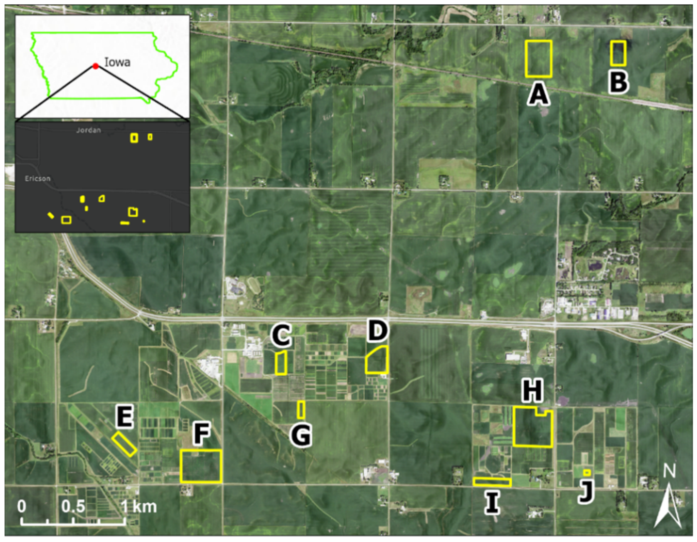
2.1. Study Fields and Soil Sampling

This research was conducted on ten agricultural fields located within a research farm near Ames, Iowa, USA, centered at approximately 93°45′28″ W 42°1′38″ N (Figure 1). Dominant soil series in these fields were Clarion (fine-loamy, mixed, superactive, mesic Aquic Hapludolls), Nicollet (fine-loamy, mixed, superactive, mesic Aquic Hapludolls), and Webster (fine- loamy, mixed, superactive, mesic Typic Endoaquolls). These soil series consist of very deep, well drained to very poorly drained soils formed on loamy till and trapped alluvium. Slope gradients ranged from 0 to 5%. Mean annual precipitation (MAP) was 700 mm. Mean air annual temperature (MAT) was 9 °C. A total of 992 soil samples, collected from a depth of 0–15 cm between 2018 and 2020 were used in this study. All samples from each of the individual fields (A-J) were collected on a single date. Sampling dates were 8 June 2018 (field B), 25 June 2018 (fields H and I), 16 July 2019 (field D), 8 June 2019 (fields F and J), 12 July 2019 (field C), 29 June 2020 (fields A, E, and G). Samples were analyzed for NO3, P2O5 (Bray-1), K2O (Neutral Ammonium Acetate method), BpH (buffer pH), SOM (soil organic matter by loss on ignition). Descriptive statistics of these samples per field and combined for all fields are provided in Table 1.

2.2. Environmental Covariates

The covariate stack encompassed 1049 spatial variables that include digital terrain analysis (DTA) (land-surface derivatives and hydrologic indicators) and RS (aerial and satellite imagery) (Table 2). All covariates were resampled to a spatial resolution of 3 m and spatially aligned. Environmental covariate values were then paired with soil lab data at the sampling locations in a GIS and transferred to a csv format for FS processing. Selected covariates were then used in respective ML algorithms to create predictive soil models.
The DTA covariates were calculated from a LiDAR-based digital elevation model (DEM) [35], using ArcGIS Pro 2.7.2 (available online: www.esri.com/software/arcgis, accessed on 27 June 2022), SAGA 2.3.2 (System for Automated Geoscientific Analysis, available online: http://www.saga-gis.org, accessed on 1 July 2022), and GRASS 7.6.1 (Geographic Resources Analysis Support System, available online: grass.osgeo.org, accessed on 3 July 2022). The LiDAR-based DEM was recorded in 2009. The r.param.scale function in GRASS was used to calculate terrain derivatives on a series of analysis scales from 9 m to 1010 m at 6 m intervals. For scale dependent analysis from SAGA GIS, the analysis scale was 9 m for a 3 m DEM and 30 m for a 10 m DEM.
RS covariates were spectral bands from the airborne, National Agriculture Imagery Program (NAIP), and Sentinel-2 Level-2A satellite imagery along with vegetation indices derived from the combinations of their spectral bands (e.g., NDVI, SAVI). All the images were downloaded from Google Earth Engine (GEE) and vegetation indices were then calculated using raster calculator functions in the GDAL package with Python. The NAIP imagery was annually recorded during the growing season. NAIP imagery was not available in 2012, 2016, and 2018 on GEE. The NAIP imagery included only red, green, and blue bands until 2009, but additionally included a near-infrared band after 2010. Only red, green, blue, and near-infrared bands with 10 m spatial resolution from Sentinel-2 were used because the other bands had coarser resolution.
The quantity of covariates used for different study fields varied. Although all DTAs were used for each field and all fields combined, the quantity of Sentinel-2 and NAIP images used in the analysis differed due to soil sampling dates. Only images from before the sampling date were used for the respective fields to set a realistic situation where soil properties are predicted for their state at time of sampling without the availability of future imagery. The presence of clouds in Sentinel-2 imagery also reduced the final quantity of images used in varying degrees for each field. As a result, fields A, E, D, and G used all 1049 covariates while the fields C, F, and J used 921, 911, and 917 covariates, respectively. Fields B, H, and I used a total of 741 covariates. For an experimental treatment considering all fields combined, 741 covariates were used to match the limitations of the fields with the earliest sampling dates.

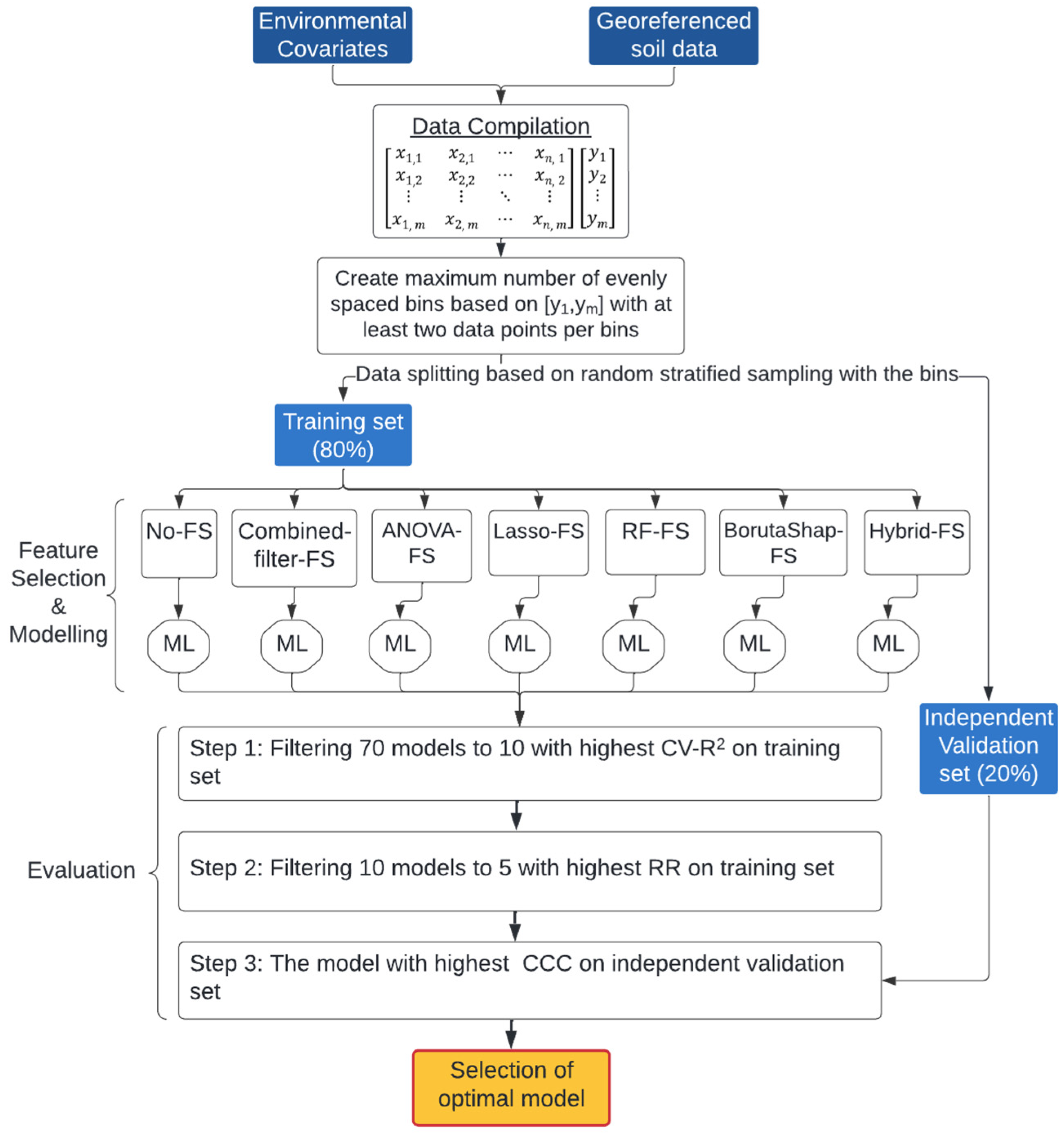
2.3. Feature Selection

Six different FS methods were applied to identify relevant covariates: (1) Combined-filter-FS, (2) ANOVA-FS, (3) BorutaShap-FS, (4) Random Forest FS (RF-FS), (5) Lasso-FS, and (6) Hybrid-FS. The Combined-filter-FS method was the combination of four filter algorithms. First, a variance threshold of 0.0001 was used to remove all low-variance covariates. This threshold was set low due to the highly decimal values of DTA covariates. Second, covariates with almost identical values were removed. Third, only one from a set of highly correlated covariates (Pearson’s correlation coefficient (r) > 0.8) were kept to avoid multicollinearity in modelling. Finally, covariates with zero for 50% or more of their values were removed to eliminate the risk of homoscedasticity in the ML models.
ANOVA-FS and BorutaShap-FS represented the filter and wrapper FS strategies, respectively. ANOVA-FS computed F-test score and p-value using an ANOVA (analysis of variance) between each covariate and the target soil property. Covariates were then ranked according to the highest F-test score and lowest p-value to select a preset quantity (K) of covariates. K values were set as 5, 10, 15, 20, 25, 30, 40, 50, 75, 100, 150, 200, 250, 300, 350, 400, 450, and 500 to have a good range of values for capturing the optimal selection and quantity of covariates for different ML models. These covariate subsets yielded 18 models. The model with the highest predictive performance according to the concordance correlation coefficient (CCC) [51] was selected for further model evaluations based on independent validation (IV; 20% of samples). BorutaShap-FS was selected as the only wrapper strategy because of high computational requirements. For BorutaShap-FS, the learning object was RF regressor with default hyperparameters. The process of running the BorutaShap-FS algorithm was automatic for returning the selected covariates.
RF-FS and Lasso-FS represented embedded FS strategies in our study. For RF-FS, feature importance was measured by mean squared error (MSE) on out-of-bag samples. The covariates whose importance was larger than the mean for all covariates were selected. SelectFromModel [52], a meta-transformer for selecting features according to importance weights, was used to return the selection of covariates from the RF regressor with default hyperparameters in Python. To implement Lasso-FS, a two-step procedure was used. First, all covariates were standardized because least squares regression fits a regression line based on Euclidean distance, thus the range of covariate values have a significant impact on the fitting process. Second, the λ (lambda) hyperparameter of the lasso regressor was tuned using GridSearchCV (10-fold). The lambda controls the L1 regularization penalty. A lambda of 0 is equivalent to ordinary least squares (OLS) regression while lambda of 1 is the full penalty. The final selection of covariates was based on the optimal lambda value according to GridSearchCV hyperparameter tuning.
The Hybrid-FS method was the sequential combination of a correlation filter with a threshold of r of 0.8 and the cross-validated recursive feature elimination (RFECV) algorithm, which is a wrapper FS strategy. The correlation filter helped eliminate correlated covariates before RFECV was run. This also helped reduce computation time of RFECV as wrapper strategies can be computationally costly. For RFECV, the learning object was Extra Trees Regressor (ETR). The optimal selection of covariates in RFECV was automatically identified based on the MSE of cross-validation.
Some configuration of parameters for the FS methods was necessary. In setting those parameters, the goal was to make the comparison between the FS methods as fair as possible while maintaining a single iteration for each FS method. Filter and some embedded (i.e., Lasso) FS strategies required their parameters to be set prior to use. Therefore, some prior exploration of parameters was necessary for these methods. For Lasso-FS and filter-based ANOVA-FS methods, heuristic search methods were used to find the optimal parameter values. However, applying similar search methods on Combined-filter-FS method was computationally costly because Combined-filter-FS method was the combination of four individual algorithms. Therefore, the setting of parameters for Combined-filter-FS method was more trial and error for estimating optimized parameters. On the other hand, wrapper-based methods (i.e., BorutaShap and RFECV used in the Hybrid-FS method) only required defining a ML algorithm to evaluate the covariate subsets during the selection process. As learning objects, decision-tree-based ML algorithms were preferred since they can run relatively quickly and tend to perform well without tuning of parameters [21]. Lastly, embedded RF-FS methods required the least amount of parameter configuration because the RF regressor method (used by RF-FS) does not require any tuning of parameters to perform well.

2.4. Machine Learning

Ten different ML algorithms were used to build models for predicting soil properties and compare FS methods by their interaction with ML algorithms. Lasso regressor [24,52,53], support vector regressor (SVR) with polynomial kernel [54], and multi-layer perceptron regressor (MLP) [55] were selected to represent classic ML algorithms. Lasso regressor is a parametric model built upon OLS with L1 regularization. SVR with polynomial kernel function discovers a flexible tube in a n-dimensional space (n depends on the number of covariates) that best fits the data with a polynomial line [56]. MLP is one of the most popular back-propagation algorithms used in artificial neural networks [57].
Six ML algorithms based on decision trees (DT) were included in the tests: RF regressor [58], extra trees regressor (ETR) [59], CatBoost [60], AdaBoost [61], LightGBM [62], and gradient boosting (GB) [63]. RF is a bagging algorithm where subsamples of the training set are randomly used to construct multiple DTs and the DTs are then combined according to the mean of their predictions. In contrast to RF, ETR builds DTs based on the whole training set and nodes are random splits. CatBoost, AdaBoost, LightGBM, and GB represented the boosting family of machine learning algorithms, where DTs are sequentially created and reweighted to improve prediction performance [64]. A key difference among these boosting algorithms is their training speed and data splitting methods at DT nodes.
As a hybrid approach to model building with ML, a voting regressor was also included in the test with the different FS methods. A voting regressor is an ensemble meta-estimator algorithm that fits several base regressors and takes the mean of individual predictions from the base learners to form the final predictions. The base regressors in this study were the nine ML algorithms above, which were then ranked according to R2 score on the validation set (20%). Validation ranking was used to weight respective model predictions in the final prediction.

2.5. Model Evaluation

Our experimental design began with applying six FS methods to the covariate stack for each target soil property and sample set, which were the individual fields plus all fields combined. The covariate stack without FS was the control treatment. Models were then built from ten ML algorithms for each of those treatments. Thus, 70 ML models were created per sample set and soil property, resulting in 3780 maps. For field J, maps were not created for BpH because all lab measurements were 7.1 (Table 1).
To simplify the evaluation process and interpretation of results, three stages of evaluation metrics were applied to identify the highest performing models and focus attention on them in subsequent stages (Figure 2). First, the models were evaluated by the R2 of 10-fold cross-validation (CV). The ten models with the highest CV-R2 score were selected for subsequent analysis based on a new metric introduced in this study to measure the robustness of the model. Here, model robustness is defined as the likelihood the model is not overfit to the training data, which was objectively evaluated by comparing the R2 for goodness-of-fit with the R2 for CV. The five models exhibiting a likelihood to be robust were subsequently evaluated for prediction performance. The model with the highest CCC [51] based on independent validation (IV; 20% of samples) was determined to be the optimal model for the respective field and soil property.
These evaluations were conducted separately for each sample set and soil property. The effect of FS method on results was evaluated by comparing the difference between the performance of the selected models produced with FS and the models produced without FS. Each field in this study contained different quantities of samples for supporting the modelling process due to varying field sizes and sample densities. These field characteristics were considered for potential correspondence with patterns observed in the performance of methods evaluated.

2.5.1. Cross-Validation

CV is a resampling method that provides a structure for creating several training and validation splits within the same dataset. In a 10-fold CV, ten models are fitted, with each fit being performed on a training set composed of 90% of the whole training set, with the remainder 10% used as a hold-out set for validation. The result of the CV is summarized as the mean performance metric across the 10 folds, which in this case was R2. As different sets of samples are used in each fitting, CV enables a comparison of stability for covariates selected as well as the generalization power of different ML algorithms [64,65,66].
High variability of performance for ML models trained with different folds in the CV process would indicate that the covariate selection is unstable or the models are being over fit [67]. A properly fitted model should be consistent in prediction performance regardless of how the data is split between training and validation sets [68]. Although the mean of the folds is commonly used to assess performance from CV [69], the mean of the folds does not describe the variability of results. Instead, there may be value in examining the standard deviation of CV results. While this evaluation would measure model stability from the perspective of changing training data, it would not necessarily differentiate issues of overfitting. If the models in all folds are consistently over fit, there is a potential for both the mean R2 to be large and the standard deviation of the R2 results to be small.

2.5.2. Robustness Ratio

One of the clearest indicators for overfitting is the decline in R2 from the original goodness-of-fit to the R2 from CV. The multiple folds in CV help protect against a result being a one-time anomaly. If the R2 results from the CV are generally much lower than the R2 from the goodness-of-fit for the original model, this would indicate that the R2 for the original model was overly optimistic for generalization due to the model being overly fit to the training data. Neither the R2 from the goodness-of-fit nor CV alone determine overfitting. A model could perform well or poorly without being overfit. Therefore, to evaluate the likelihood that a model is overfit—which is to say the likelihood that prediction performance will be robust regardless of the data used for training—a metric is needed that compares goodness-of-fit with CV. For this purpose, a robustness ratio (RR) is proposed (Equation (1)), whereby the ratio between a 10-fold CV’s R2 score and the goodness-of-fit (training R2 score) is used to quantify the dependence of model performance on the training set used to construct the model (i.e., overfitting).
R R = m e a n   R 2   o f   C V R 2   o f   g o o d n e s s o f f i t

2.5.3. Independent Validation

To test for prediction performance, the respective models are evaluated by IV using CCC instead of R2. The major difference between CV and IV is that CV does not directly evaluate the performance of the model used to make predictions because a different model is created with every fold of CV. CCC is used for IV instead of R2 because in the final assessment of prediction performance, the relationship of interest is that between the observed and the predicted. The relationship between observed and predicted should be evaluated against a 1:1 line, not a new model fit to the relationship between observed and predicted [70].

3. Results

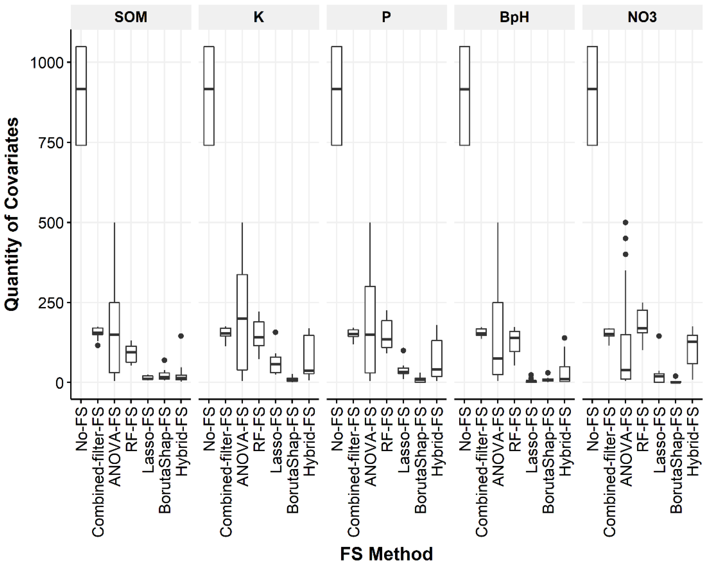
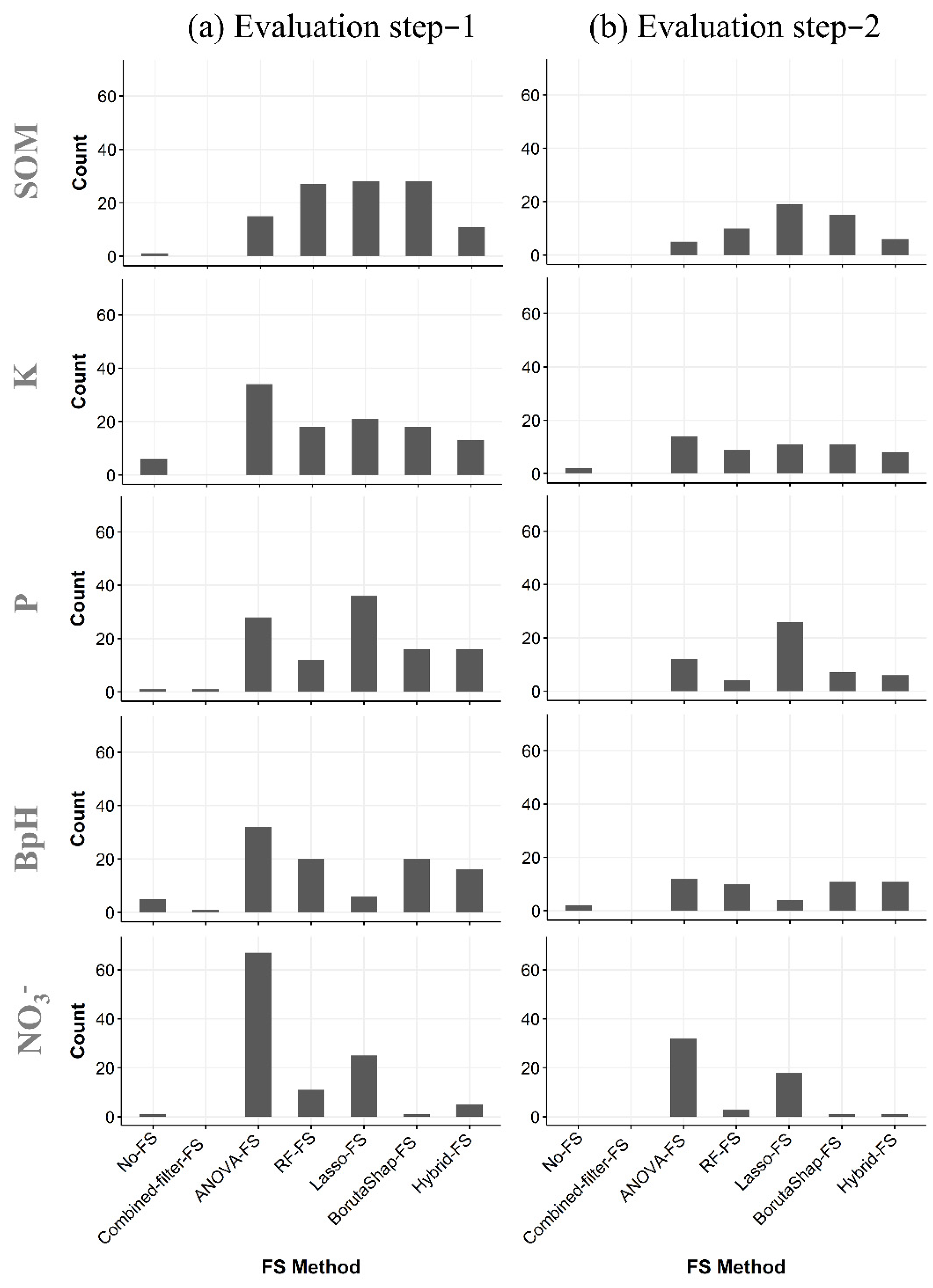
3.1. Quantity of Covariates Selected

All FS strategies accomplished a decrease in the quantity of covariates to be used in modelling relative to the covariate stacks without FS (Figure 3). Full covariate stacks had a range of 741 to 1049 covariates among different sample sets, depending on the availability of imagery covering the sample set area. Overall, FS methods consistently reduced the covariate stack to less than half of the original quantity. The largest reduction in covariate stack size was typically made by BorutaShap-FS. An exception to this was for BpH, where the median quantity of covariates for Lasso-FS was five, while this value was nine for BorutaShap-FS.
Lasso-FS and Hybrid-FS followed BorutaShap-FS in terms of yielding the largest reduction in covariate stack size. These two methods output similar quantities of covariates among soil properties except for K and NO3. The Lasso-FS method resulted in a much smaller median quantity of covariates selected (20) compared to Hybrid-FS (128) for NO3. For K, Lasso-FS and Hybrid-FS had medians of 58 and 37 covariates selected, respectively.
ANOVA-FS, Combined-filter-FS, and RF-FS resulted in less reduced covariate stacks. For Combined-filter-FS, the median quantity of covariates was around 153 for all soil properties, while the quantity of covariates selected varied by soil property with RF-FS and ANOVA-FS. The median quantity of covariates ranged from 95 (SOM) to 169 (NO3) for RF-FS. The highest variability in quantity of covariates selected among different soil properties was with ANOVA-FS as the median covariate quantities ranged from 40 (NO3) to 200 (K). The quantity of covariates selected was also highly variable with ANOVA-FS across the different sample sets.

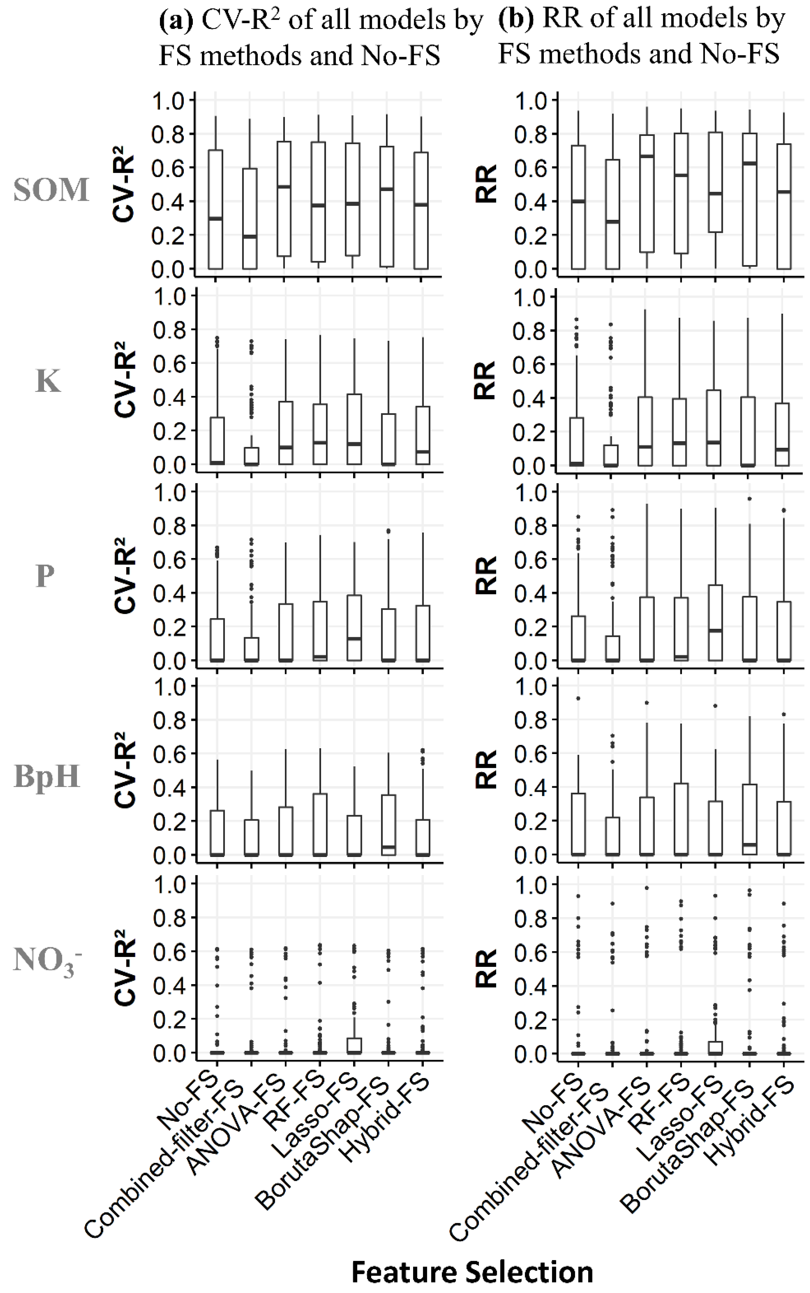
3.2. Cross-Validation
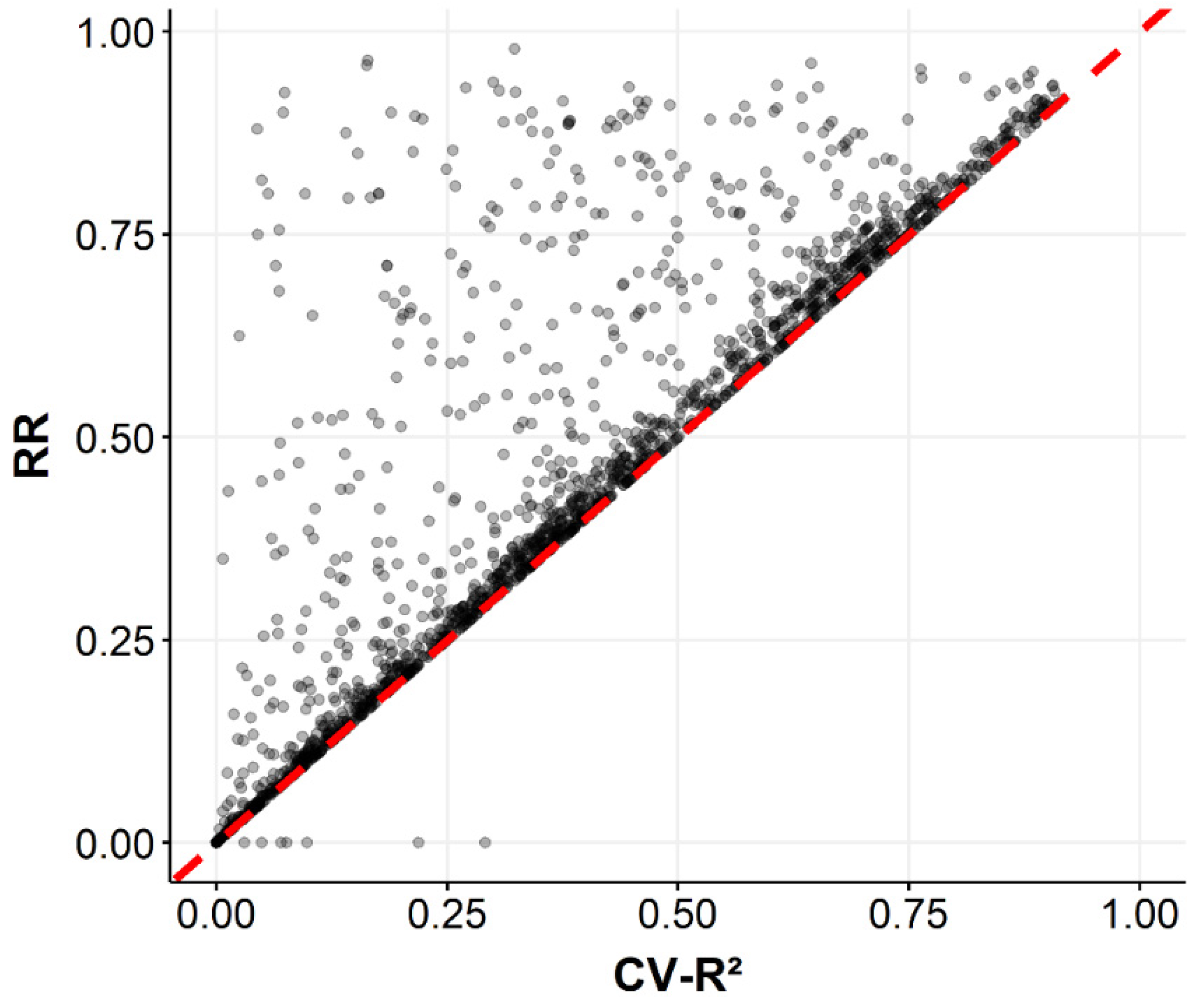
Models built from covariate stacks reduced by FS methods mostly performed better in cross-validation than those built without FS (Figure 4a) for all soil properties. No-FS had a value of zero for the median CV-R2 for all soil properties except for SOM, which was 0.31. However, models built from covariate stacks selected by Combined-filter-FS were generally even worse than No-FS for CV-R2. NO3 was particularly challenging for producing predictive models, where the median CV-R2 for No-FS and all FS methods was zero.
Figure 5a shows the frequency of models from different FS methods that advanced through the first step of the evaluation. Differences between No-FS and FS methods were highlighted because models with No-FS in this step were less frequently chosen by the criteria of being in the top ten of CV-R2 for the respective sample sets and soil properties. RF-FS, Lasso-FS, and BorutaShap-FS produced the most frequently chosen models for SOM. However, ANOVA-FS produced the most frequently selected models for most other soil properties. P was unique in that Lasso-FS produced the most top performing models in terms of CV-R2, with ANOVA-FS producing the second most top performing models.

3.3. Robustness

Patterns between CV (Figure 4a) and RR (Figure 4b) were similar, which suggests stronger CV performance could be connected to RR performance (Figure 6). The correlation between these metrics was evaluated (r = 0.9) and CV performance appeared to indicate a minimum RR value. However, several models had higher RR scores than the CV-R2 score might predict. Those models with higher RR scores were those that had less of a decrease in R2 from the original model training compared to the CV, which would indicate less overfitting.
In the second step of the evaluation, models from some FS methods remained competitive, while others were more often cut due to lower performance in terms of RR. The difference between Lasso-FS and other FS methods became larger for SOM and BpH in this second round of criteria, suggesting that Lasso-FS methods were producing models that were less overfit. Although ANOVA-FS had the highest frequencies in the first step for K, BpH and NO3, the difference between ANOVA-FS and other FS methods became smaller. While models produced from ANOVA-FS-based covariate stacks were still the most frequently chosen for those soil properties, this pattern also indicates that some of the ANOVA-FS-based models with high CV-R2 were not as robust as models coming from other FS methods. All remaining models from Combined-filter-FS were eliminated in this second step of the evaluation process. However, some of the few models produced from No-FS covariate stacks that passed the first step, also passed this second step for K and BpH.

3.4. Independent Validation

Models produced from covariate stacks reduced by FS methods outperformed models built from covariate stacks without FS in most cases (Figure 7 and Figure 8). IV-CCC scores for the final models were higher than No-FS models for nine (SOM), eight (K), six (P), five (BpH), and all (NO3) sample sets. For SOM, Lasso-FS and Hybrid-FS were the most common optimal FS methods among the sample sets. There was no single optimal FS method among the sample sets for K. However, BorutaShap-FS, ANOVA-FS, RF-FS, Lasso-FS were commonly optimal FS methods among the sample sets.
Lasso-FS and ANOVA-FS were the most frequently chosen FS methods among the sample sets for P and NO3. Although ANOVA-FS was the chosen FS method for eight of the sample sets for NO3, the models built from ANOVA-FS usually showed signs of overfitting because these models had CV-R2 and RR of zero. Similar situations were observed for the other soil properties and sample sets where a model built from an ANOVA-FS-based covariate stack was identified as the best performing model. These sample sets typically had relatively smaller quantities of samples. With ANOVA-FS, sample sets with larger sample quantities (e.g., field D for K, all fields for P and NO3) usually had relatively higher performance for CV-R2 and RR compared to the sample sets with smaller sample sizes.
ML algorithms that use decision tree approaches (i.e., ETR, boosting algorithms, and RF), paired with the FS methods in this study, generally built the top performing models for all soil properties except NO3. In the case of NO3, boosting ML and ETR led to the optimal models in one and two sample sets, respectively, without considering the sample sets with obvious indication of overfitting (RR = 0). For P, the decision-tree-based ML algorithms produced the optimal models for one sample set (ETR) and eight sample sets (boosting). Boosting and ETR were optimal models in seven and three sample sets, respectively for both K and BpH. Similarly, boosting algorithms yielded optimal models in seven sample sets for SOM, while RF and ETR were optimal ML models in two and one fields, respectively.

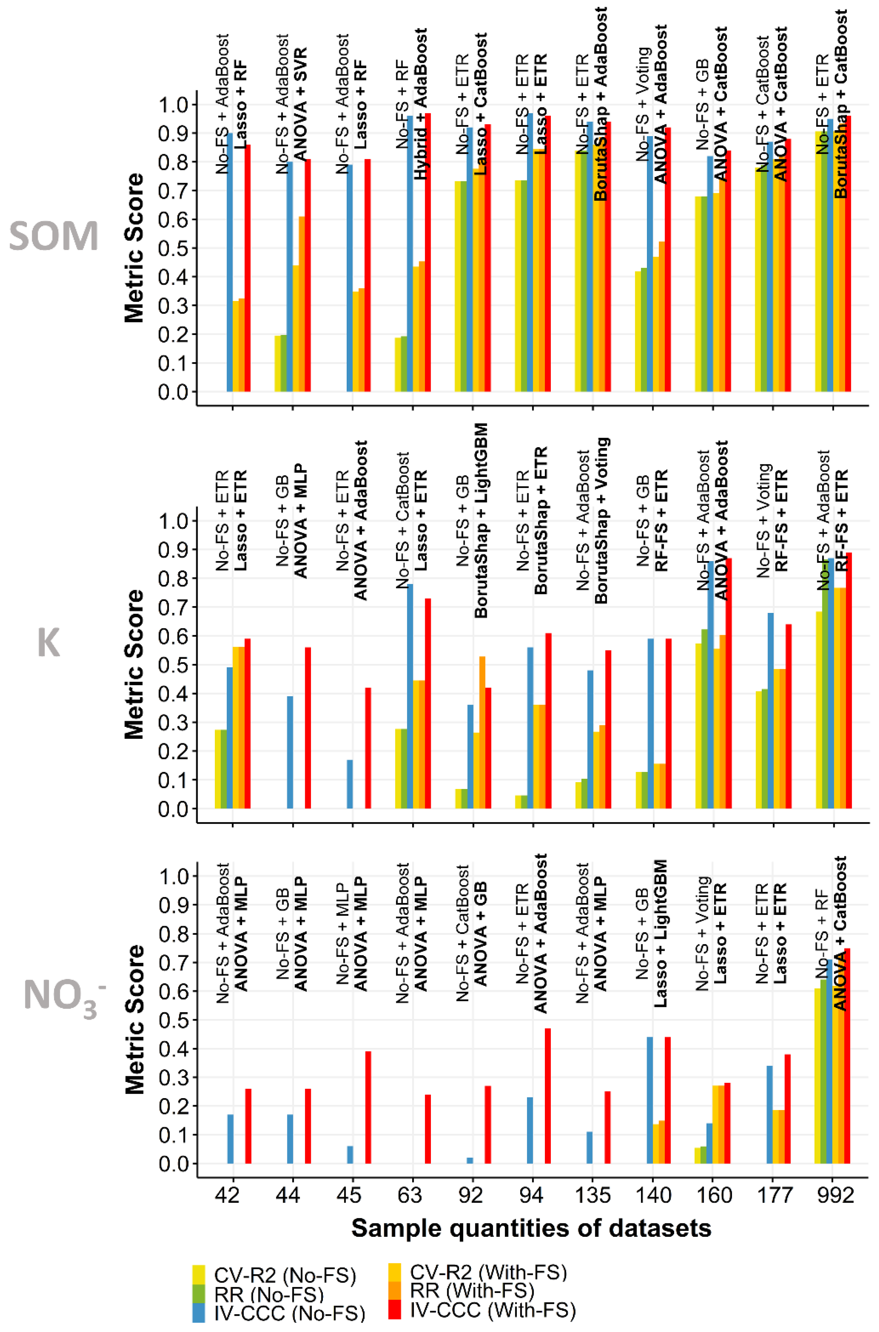
3.5. Effect of Sample Quantity

The effect of sample quantity on the covariates selected and model performance was investigated for the quantities in the original sample sets, which were based on separate fields and all fields combined. Although a general pattern of more covariates being selected by FS methods with larger sample sets could be observed, this correlation was stronger for some FS methods than others. This relationship was strongest for Combined-filter-FS, Lasso-FS, and BorutaShap-FS, while RF-FS, ANOVA-FS and Hybrid-FS had weaker correlations. For Combined-filter-FS, the quantity of covariates selected tended to increase with increasing sample quantity (0.51 ≤ r ≤ 0.72 for different soil properties). While the range of r values was from 0.07 (BpH) to 0.87 (K) for Lasso-FS, BorutaShap-FS had a range from 0.25 (P) to 0.60 (SOM). Intriguingly, RF-FS had a negative relationship between quantity of samples and covariates selected for SOM (r = −0.56). For the other soil properties, there was no relationship for RF-FS.
IV-CCC results appeared to be higher with more samples in a sample set, but this relationship was weakly correlated for each of the FS methods (0.09 ≤ r ≤ 0.14). Examples of situations that disrupted this potential pattern can be seen in Figure 7 and Figure 8, where some fields with smaller quantities outperformed fields with larger sample quantities. For example, field J with 63 samples had the highest IV-CCC for SOM (0.96) among all sample sets even though that field had one of the smaller quantities of samples. However, the sample set consisting of samples from all individual fields combined was usually among the highest for all metrics. Nonetheless, a noteworthy observation about the all fields sample set was that FS did not substantially affect the scores of evaluation metrics in the final model compared to its counterpart with No-FS. Besides, small sample quantities seemed to contribute to low RR and CV for most sample sets for NO3. Sample quantities smaller than 140 was not enough to create models with relatively high CV and RR for NO3, while this situation was less common for the other soil properties.

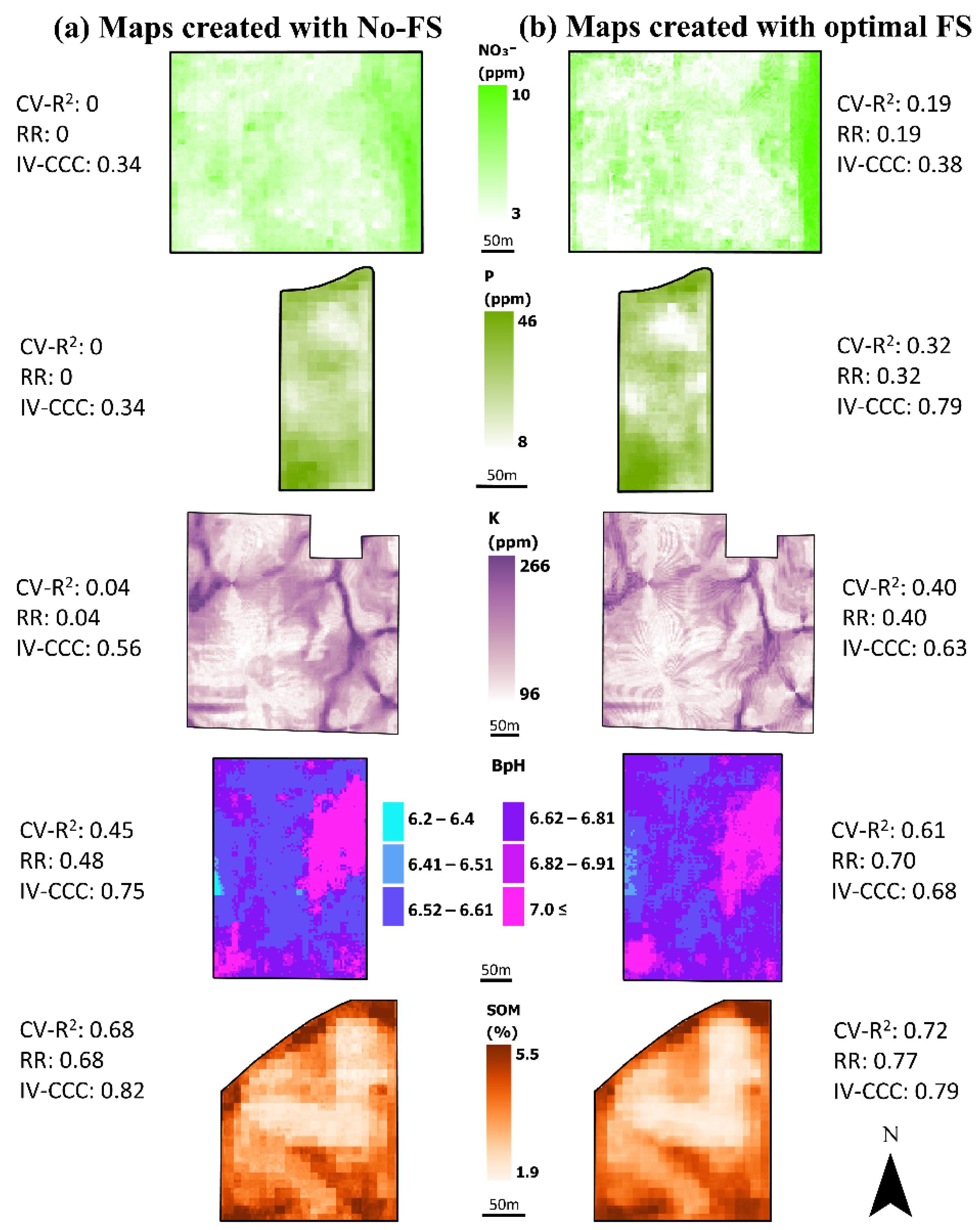
3.6. Comparison of Spatial Patterns in Maps

Digital soil maps developed with the full covariate stack tended to be smoother than the maps created by using FS with exceptions in some fields (e.g., SOM map in field D). Despite differences observed in the evaluation of the models’ prediction performance, all maps produced from covariate stacks reduced by FS had similar patterns to their No-FS counterparts. Figure 9 presents some examples comparing maps developed with and without FS.

4. Discussion

4.1. Optimal FS Strategies

Although DSM has become a common practice for creating soil information, its reliance on predictive models creates skepticism about the accuracy and robustness of digital soil maps [70]. In this study, use of a three-tiered evaluation approach that incorporates a novel metric for robustness (RR) beyond the commonly used CV approach for evaluating model performance. This process helped narrow the pool of possible models for desirable characteristics of prediction power without being overfit. As determined by the evaluation procedure, the optimal models outperformed the baseline models with No-FS.
Filter and hybrid strategies rarely produced the optimal models. ANOVA-FS, representing the filter strategy, frequently produced models with relatively high CV-R2 scores. However, for many of the ANOVA-FS-based models the RR score indicated those models were overfit, especially for smaller sample quantities and certain soil properties (e.g., NO3). Although hybrid FS strategies have been found promising in other studies [14,26], this was rarely the case in our study. The Hybrid-FS method in our study outperformed other FS methods for only a few sample sets when predicting BpH and SOM. However, other researchers [26] have found promising results for hybrid-based FS methods for mapping SOM. Lower performance of the Hybrid-FS method in our study could be due to the effect of combining correlation filter and RFECV to create the Hybrid-FS method.
Embedded and wrapper strategies were frequently the optimal FS methods. Better performance of wrapper and embedded FS strategies in our study can be attributed to their ability to capture non-linear data relationships [71,72], which are frequently found in complicated soil-landscape relationships [12,73]. Most literature that has compared filter FS strategies with embedded and wrapper strategies [11,26,27,74] also reached similar conclusions. Wrapper and embedded FS strategies usually outperformed filter FS strategies with smaller sample quantities [6,26,28,32,74]. The addition of bootstrapping to embedded and wrapper FS strategies could also be effective in making these FS methods more powerful relative to filter-based FS methods [75]. In our study, this was the case for the wrapper-based BorutaShap-FS method where the learning object was the RF regressor, which uses bootstrap samples in its inner dynamics.

4.2. Optimal FS-ML Combinations

Decision-tree-based algorithms (e.g., ETR, RF, and CatBoost) coupled with Lasso-FS, RF-FS, and BorutaShap-FS frequently led to the optimal models. Some of the decision-tree-based ML algorithms used in this study were based on bagging (i.e., RF) and boosting (i.e., CatBoost, AdaBoost, LightGBM, and GB) techniques. Bagging is an advantageous technique as it decreases the variance and improves the stability of predictions by combining predictions from different decision trees [76]. Besides, both bagging and boosting algorithms are less sensitive to sample size [77]. Boosting algorithms have another advantage that they iteratively attempt to improve prediction accuracy, which give boosting algorithms the ability to self-analyze the prediction errors and improve the predictions [78].
In the DSM literature, decision-tree-based algorithms have been compared frequently but with mixed results. Meier et al. [79] compared classification performance of eight ML algorithms (e.g., SVM with linear kernel, SVM with polynomial kernel, XGboost, and RF) with a hybrid-based FS method, which was a combination of correlation filter with a threshold of r = 0.98 and RFE for classifying soil types. They found that XGboost usually responded better to the hybrid-based FS than the SVM with linear kernel. Similarly, Chen et al. [26] showed XGBoost ML responded slightly better to different FS categories (i.e., filter, hybrid, embedded, and wrapper) than RF for modelling SOM. In contrast, Xiong et al. [3] found that bagging-based ML can perform better than boosting-based ML as they demonstrated RF performed slightly better than a boosted regression tree ML with wrapper-based FS methods.
The ML algorithms that rarely led to the optimal models, regardless of the FS method with which they were paired, were the classical ML algorithms such as SVR, MLP, and lasso regressor. MLP is known to be vulnerable to poor performance with small quantities of sample points and needing thousands of samples to produce reliable models [70,80]. Given the relatively small quantity of samples that are common for field-scale soil mapping, as was the case in this study, poor performance of MLP was expected. Likewise, SVR can be more prone to overfitting with fewer samples relative to decision-tree-based ML algorithms [70]. This may have contributed to SVR’s mediocre performance for many of the sample sets tested. Lasso regressor was never a part of the optimal FS and ML combinations among sample sets and soil properties. The lower performance of this ML algorithm could be due to the presence of complex relationships between covariates and target variables found in our datasets, which could not be explained by a linear model like lasso regression.

5. Conclusions

Six types of FS methods from four categories (filter, wrapper, embedding, and hybrid) were compared for their effectiveness in selecting relevant covariates from an exhaustive set of 1049 environmental covariates. These FS methods were tested for building ML-based models predicting the soil fertility properties SOM, K, P, BpH, and NO3 in ten crop research fields. In this context, a metric of robustness was proposed to assist in model evaluation. The new robustness ratio (RR) was designed to measure the reliance of model performance on the samples used for training as an indicator of over-fitting. Using RR in model evaluation process made it easier to find optimal combinations of FS and ML that can enhance DSM performance over models built from full covariate stacks.
Models produced from covariate stacks reduced by FS methods were less likely to be overfit and tended to have better performance in IV-CCC. Although there was no single optimal FS method among sample sets or soil properties, wrapper and embedded FS strategies produced the optimal model more frequently than the hybrid and filter FS strategies. The Combined-filter method was the only FS method that had worse performance than No-FS-based models for most cases. Decision-tree-based ML algorithms (e.g., ETR, GB, and RF), paired with the FS methods, usually built the top performing models for all soil properties. However, predicting NO3 was particularly challenging compared to the other soil properties regardless of FS method and ML algorithm used.

Author Contributions

Conceptualization, B.A.M.; methodology, C.F.; software, C.F.; validation, B.A.M. and C.F.; formal analysis, B.A.M. and C.F.; investigation, C.F. and B.A.M.; resources, B.A.M.; data curation, C.F.; writing—original draft preparation, C.F.; writing—review and editing, C.F. and B.A.M.; visualization, C.F.; supervision, B.A.M.; project administration, B.A.M.; funding acquisition, B.A.M. All authors have read and agreed to the published version of the manuscript.

Funding

This research received no external funding.

Data Availability Statement

Sentinel-2 and NAIP imagery bands can be downloaded from https://earthengine.google.com/ (accessed on 5 July 2022). Lidar DEMs were downloaded from https://geodata.iowa.gov/ (accessed on 6 July 2022).

Acknowledgments

This work would not have been possible without the cooperation of several research groups within the Department of Agronomy at Iowa State University. Special thanks to the A.K. Singh Soybean Breeding and Genetics Group and the Geospatial Laboratory for Soil Informatics. Support for Caner Ferhatoglu was provided by the Department of Agronomy at Iowa State University.

Conflicts of Interest

The authors declare no conflict of interest.

References

  1. Minasny, B.; McBratney, A.B. Digital Soil Mapping: A Brief History and Some Lessons. Geoderma 2016, 264, 301–311. [Google Scholar] [CrossRef]
  2. McBratney, A.B.; Santos, M.L.M.; Minasny, B. On Digital Soil Mapping. Geoderma 2003, 117, 3–52. [Google Scholar] [CrossRef]
  3. Xiong, X.; Grunwald, S.; Myers, D.B.; Kim, J.; Harris, W.G.; Comerford, N.B. Holistic Environmental Soil-Landscape Modeling of Soil Organic Carbon. Environ. Model. Softw. 2014, 57, 202–215. [Google Scholar] [CrossRef]
  4. Brungard, C.W.; Boettinger, J.L.; Duniway, M.C.; Wills, S.A.; Edwards, T.C. Machine Learning for Predicting Soil Classes in Three Semi-Arid Landscapes. Geoderma 2015, 239, 68–83. [Google Scholar] [CrossRef] [Green Version]
  5. Kuhn, M.; Johnson, K. Applied Predictive Modeling; Springer: New York, NY, USA, 2013; ISBN 9781461468493. [Google Scholar]
  6. Flynn, T.; de Clercq, W.; Rozanov, A.; Clarke, C. High-Resolution Digital Soil Mapping of Multiple Soil Properties: An Alternative to the Traditional Field Survey? S. Afr. J. Plant Soil 2019, 36, 237–247. [Google Scholar] [CrossRef]
  7. Van Dijk, A.D.J.; Kootstra, G.; Kruijer, W.; de Ridder, D. Machine Learning in Plant Science and Plant Breeding. iScience 2021, 24, 101890. [Google Scholar] [CrossRef]
  8. Hesami, M.; Jones, A.M.P. Application of Artificial Intelligence Models and Optimization Algorithms in Plant Cell and Tissue Culture. Appl. Microbiol. Biotechnol. 2020, 104, 9449–9485. [Google Scholar] [CrossRef]
  9. Singh, A.; Ganapathysubramanian, B.; Singh, A.K.; Sarkar, S. Machine Learning for High-Throughput Stress Phenotyping in Plants. Trends Plant Sci. 2016, 21, 110–124. [Google Scholar] [CrossRef] [Green Version]
  10. Bellman, R.; Kalaba, R.E. Dynamic Programming and Modern Control Theory; Citeseer: Princeton, NJ, USA, 1965; Volume 81. [Google Scholar]
  11. Chandrashekar, G.; Sahin, F. A Survey on Feature Selection Methods. Comput. Electr. Eng. 2014, 40, 16–28. [Google Scholar] [CrossRef]
  12. Li, J.; Cheng, K.; Wang, S.; Morstatter, F.; Trevino, R.P.; Tang, J.; Liu, H. Feature Selection: A Data Perspective. ACM Comput. Surv. 2017, 50, 1–45. [Google Scholar] [CrossRef]
  13. Bolón-Canedo, V.; Alonso-Betanzos, A. Ensembles for Feature Selection: A Review and Future Trends. Inf. Fusion 2019, 52, 1–12. [Google Scholar] [CrossRef]
  14. Wadoux, A.M.J.C.; Minasny, B.; McBratney, A.B. Machine Learning for Digital Soil Mapping: Applications, Challenges and Suggested Solutions. Earth-Sci. Rev. 2020, 210, 103359. [Google Scholar] [CrossRef]
  15. Yu, L.; Liu, H. Feature Selection for High-Dimensional Data: A Fast Correlation-Based Filter Solution. In Proceedings of the 20th International Conference on Machine Learning (ICML-03), Washington, DC, USA, 21–24 August 2003; pp. 856–863. [Google Scholar]
  16. De la Iglesia, B. Evolutionary Computation for Feature Selection in Classification Problems. WIREs Data Min. Knowl. Discov. 2013, 3, 381–407. [Google Scholar] [CrossRef]
  17. Seijo-Pardo, B.; Porto-Díaz, I.; Bolón-Canedo, V.; Alonso-Betanzos, A. Ensemble Feature Selection: Homogeneous and Heterogeneous Approaches. Knowl.-Based Syst. 2017, 118, 124–139. [Google Scholar] [CrossRef]
  18. Keany, E. BorutaShap: A Wrapper Feature Selection Method Which Combines the Boruta Feature Selection Algorithm with Shapley Values; Zenodo: Geneva, Switzerland, 2020. [Google Scholar]
  19. Chieregato, M.; Frangiamore, F.; Morassi, M.; Baresi, C.; Nici, S.; Bassetti, C.; Bnà, C.; Galelli, M. A Hybrid Machine Learning/Deep Learning COVID-19 Severity Predictive Model from CT Images and Clinical Data. Sci. Rep. 2022, 12, 4329. [Google Scholar] [CrossRef] [PubMed]
  20. Keany, E.; Bessardon, G.; Gleeson, E. Using Machine Learning to Produce a Cost-Effective National Building Height Map of Ireland to Categorise Local Climate Zones. Adv. Sci. Res. 2022, 19, 13–27. [Google Scholar] [CrossRef]
  21. Kursa, M.B.; Rudnicki, W.R. Feature Selection with the Boruta Package. J. Stat. Softw. 2010, 36, 1–13. [Google Scholar] [CrossRef] [Green Version]
  22. Lundberg, S.M.; Lee, S.I. A Unified Approach to Interpreting Model Predictions. Adv. Neural Inf. Process. Syst. 2017, 2017, 4766–4775. [Google Scholar]
  23. Shapley, L.S. A Value for N-Person Games. In Contributions to the Theory of Games; Princeton University Press: Princeton, NJ, USA, 1953; Volume 2, pp. 307–317. [Google Scholar]
  24. Tibshirani, R. Regression Shrinkage and Selection Via the Lasso. J. R. Stat. Soc. Ser. B Methodol. 1996, 58, 267–288. [Google Scholar] [CrossRef]
  25. Shi, Y.; Zhao, J.; Song, X.; Qin, Z.; Wu, L.; Wang, H.; Tang, J. Hyperspectral Band Selection and Modeling of Soil Organic Matter Content in a Forest Using the Ranger Algorithm. PLoS ONE 2021, 16, e0253385. [Google Scholar] [CrossRef]
  26. Chen, Y.; Ma, L.; Yu, D.; Zhang, H.; Feng, K.; Wang, X.; Song, J. Comparison of Feature Selection Methods for Mapping Soil Organic Matter in Subtropical Restored Forests. Ecol. Indic. 2022, 135, 108545. [Google Scholar] [CrossRef]
  27. Behrens, T.; Zhu, A.-X.; Schmidt, K.; Scholten, T. Multi-Scale Digital Terrain Analysis and Feature Selection for Digital Soil Mapping. Geoderma 2010, 155, 175–185. [Google Scholar] [CrossRef]
  28. Campos, A.R.; Giasson, E.; Costa, J.J.F.; Machado, I.R.; da Silva, E.B.; Bonfatti, B.R. Selection of Environmental Covariates for Classifier Training Applied in Digital Soil Mapping. Rev. Bras. Ciênc. Solo 2019, 42, 1–15. [Google Scholar] [CrossRef] [Green Version]
  29. Hong, Y.; Chen, S.; Chen, Y.; Linderman, M.; Mouazen, A.M.; Liu, Y.; Guo, L.; Yu, L.; Liu, Y.; Cheng, H.; et al. Comparing Laboratory and Airborne Hyperspectral Data for the Estimation and Mapping of Topsoil Organic Carbon: Feature Selection Coupled with Random Forest. Soil Tillage Res. 2020, 199, 104589. [Google Scholar] [CrossRef]
  30. Yang, R.-M.; Liu, L.-A.; Zhang, X.; He, R.-X.; Zhu, C.-M.; Zhang, Z.-Q.; Li, J.-G. The Effectiveness of Digital Soil Mapping with Temporal Variables in Modeling Soil Organic Carbon Changes. Geoderma 2022, 405, 115407. [Google Scholar] [CrossRef]
  31. Luo, C.; Zhang, X.; Wang, Y.; Men, Z.; Liu, H. Regional Soil Organic Matter Mapping Models Based on the Optimal Time Window, Feature Selection Algorithm and Google Earth Engine. Soil Tillage Res. 2022, 219, 105325. [Google Scholar] [CrossRef]
  32. Lu, Y.; Liu, F.; Zhao, Y.; Song, X.; Zhang, G. An Integrated Method of Selecting Environmental Covariates for Predictive Soil Depth Mapping. J. Integr. Agric. 2019, 18, 301–315. [Google Scholar] [CrossRef]
  33. Domenech, M.B.; Amiotti, N.M.; Costa, J.L.; Castro-Franco, M. Prediction of Topsoil Properties at Field-Scale by Using C-Band SAR Data. Int. J. Appl. Earth Obs. Geoinf. 2020, 93, 102197. [Google Scholar] [CrossRef]
  34. Wang, S.-H.; Lu, H.-L.; Zhao, M.-S.; Zhou, L.-M. Assessing soil pH in Anhui Province based on different features mining methods combined with generalized boosted regression models. Ying Yong Sheng Tai Xue Bao J. Appl. Ecol. 2020, 31, 3509–3517. [Google Scholar] [CrossRef]
  35. Iowa Geospatial Data. Available online: https://geodata.iowa.gov/ (accessed on 28 June 2022).
  36. Ashley, M.D.; Rea, J. Seasonal Vegetation Differences from ERTS Imagery; American Society of Photogrammetry: Falls Church, VA, USA, 1975; Volume 41. [Google Scholar]
  37. Huete, A.R. A Soil-Adjusted Vegetation Index (SAVI). Remote Sens. Environ. 1988, 25, 295–309. [Google Scholar] [CrossRef]
  38. Richardson, A.J.; Wiegand, C. Distinguishing Vegetation from Soil Background Information. Photogramm. Eng. Remote Sens. 1977, 43, 1541–1552. [Google Scholar]
  39. Xiaoqin, W.; Miaomiao, W.; Shaoqiang, W.; Yundong, W. Extraction of Vegetation Information from Visible Unmanned Aerial Vehicle Images. Trans. Chin. Soc. Agric. Eng. 2015, 31, 152–159. [Google Scholar]
  40. Qi, J.; Chehbouni, A.; Huete, A.R.; Kerr, Y.H.; Sorooshian, S. A Modified Soil Adjusted Vegetation Index. Remote Sens. Environ. 1994, 48, 119–126. [Google Scholar] [CrossRef]
  41. Gitelson, A.A.; Gritz, Y.; Merzlyak, M.N. Relationships between Leaf Chlorophyll Content and Spectral Reflectance and Algorithms for Non-Destructive Chlorophyll Assessment in Higher Plant Leaves. J. Plant Physiol. 2003, 160, 271–282. [Google Scholar] [CrossRef] [PubMed]
  42. Tucker, C.J. Red and Photographic Infrared Linear Combinations for Monitoring Vegetation. Remote Sens. Environ. 1979, 8, 127–150. [Google Scholar] [CrossRef] [Green Version]
  43. Travis, M.R. VIEWIT: Computation of Seen Areas, Slope, and Aspect for Land-Use Planning; Department of Agriculture, Forest Service, Pacific Southwest Forest and Range Experiment Station: Albany, CA, USA, 1975; Volume 11.
  44. Tarboton, D.G. A New Method for the Determination of Flow Directions and Upslope Areas in Grid Digital Elevation Models. Water Resour. Res. 1997, 33, 309–319. [Google Scholar] [CrossRef] [Green Version]
  45. Costa-Cabral, M.C.; Burges, S.J. Digital Elevation Model Networks (DEMON): A Model of Flow over Hillslopes for Computation of Contributing and Dispersal Areas. Water Resour. Res. 1994, 30, 1681–1692. [Google Scholar] [CrossRef]
  46. Evans, I.S. An Integrated System of Terrain Analysis and Slope Mapping. Z. Für Geomorphol. Suppl. Stuttg. 1980, 36, 274–295. [Google Scholar]
  47. Heerdegen, R.G.; Beran, M.A. Quantifying Source Areas through Land Surface Curvature and Shape. J. Hydrol. 1982, 57, 359–373. [Google Scholar] [CrossRef]
  48. Bauer, J.; Rohdenburg, H.; Bork, H. Ein Digitales Reliefmodell als Vorraussetzung für ein Deterministisches Modell der Wasser-und Stoff-Flüsse. Landsch. Landsch. 1985, 10, 1–15. [Google Scholar]
  49. Zevenbergen, L.W.; Thorne, C.R. Quantitative Analysis of Land Surface Topography. Earth Surf. Process. Landf. 1987, 12, 47–56. [Google Scholar] [CrossRef]
  50. Haralick, R.M. Ridges and Valleys on Digital Images. Comput. Vis. Graph. Image Process. 1983, 22, 28–38. [Google Scholar] [CrossRef]
  51. Lin, L.I.-K. A Concordance Correlation Coefficient to Evaluate Reproducibility. Biometrics 1989, 45, 255–268. [Google Scholar] [CrossRef] [PubMed]
  52. Pedregosa, F.; Varoquaux, G.; Gramfort, A.; Michel, V.; Thirion, B.; Grisel, O.; Blondel, M.; Prettenhofer, P.; Weiss, R.; Dubourg, V. Scikit-Learn: Machine Learning in Python. J. Mach. Learn. Res. 2011, 12, 2825–2830. [Google Scholar]
  53. Jonas, R.; Cook, J. Lasso Regression. Br. J. Surg. 2018, 105, 1348. [Google Scholar]
  54. Drucker, H.; Burges, C.J.; Kaufman, L.; Smola, A.; Vapnik, V. Support Vector Regression Machines. Adv. Neural Inf. Process. Syst. 1996, 9, 155–161. [Google Scholar]
  55. Rosenblatt, F. The Perceptron: A Probabilistic Model for Information Storage and Organization in the Brain. Psychol. Rev. 1958, 65, 386. [Google Scholar] [CrossRef] [Green Version]
  56. Awad, M.; Khanna, R. Support Vector Regression. In Efficient Learning Machines: Theories, Concepts, and Applications for Engineers and System Designers; Awad, M., Khanna, R., Eds.; Apress: Berkeley, CA, USA, 2015; pp. 67–80. ISBN 9781430259909. [Google Scholar]
  57. Schmidhuber, J. Deep Learning in Neural Networks: An Overview. Neural Netw. 2015, 61, 85–117. [Google Scholar] [CrossRef] [Green Version]
  58. Breiman, L. Bagging Predictors. Mach. Learn. 1996, 24, 123–140. [Google Scholar] [CrossRef] [Green Version]
  59. Geurts, P.; Ernst, D.; Wehenkel, L. Extremely Randomized Trees. Mach. Learn. 2006, 63, 3–42. [Google Scholar] [CrossRef] [Green Version]
  60. Dorogush, A.V.; Ershov, V.; Gulin, A. CatBoost: Gradient Boosting with Categorical Features Support. arXiv 2018, arXiv:1810.11363. [Google Scholar]
  61. Freund, Y.; Schapire, R.E. Experiments with a New Boosting Algorithm; Citeseer: Princeton, NJ, USA, 1996; Volume 96, pp. 148–156. [Google Scholar]
  62. Ke, G.; Meng, Q.; Finley, T.; Wang, T.; Chen, W.; Ma, W.; Ye, Q.; Liu, T.-Y. Lightgbm: A Highly Efficient Gradient Boosting Decision Tree. Adv. Neural Inf. Process. Syst. 2017, 30, 3146–3154. [Google Scholar]
  63. Friedman, J.H. Greedy Function Approximation: A Gradient Boosting Machine. Ann. Stat. 2001, 29, 1189–1232. [Google Scholar] [CrossRef]
  64. Oshiro, T.M.; Perez, P.S.; Baranauskas, J.A. How Many Trees in a Random Forest? In Proceedings of the International Workshop on Machine Learning and Data Mining in Pattern Recognition; Springer: Berlin/Heidelberg, Germany, 2012; pp. 154–168. [Google Scholar]
  65. Refaeilzadeh, P.; Tang, L.; Liu, H. Cross-Validation. Encycl. Database Syst. 2009, 5, 532–538. [Google Scholar]
  66. Arlot, S.; Celisse, A. A Survey of Cross-Validation Procedures for Model Selection. Stat. Surv. 2010, 4, 40–79. [Google Scholar] [CrossRef]
  67. Kelcey, B. Covariate Selection in Propensity Scores Using Outcome Proxies. Multivar. Behav. Res. 2011, 46, 453–476. [Google Scholar] [CrossRef]
  68. Browne, M.W. Cross-Validation Methods. J. Math. Psychol. 2000, 44, 108–132. [Google Scholar] [CrossRef] [Green Version]
  69. Berrar, D. Cross-Validation; Tokyo Institute of Technology: Tokyo, Japan, 2019. [Google Scholar]
  70. Khaledian, Y.; Miller, B.A. Selecting Appropriate Machine Learning Methods for Digital Soil Mapping. Appl. Math. Model. 2020, 81, 401–418. [Google Scholar] [CrossRef]
  71. Cheng, T.H.; Wei, C.P.; Tseng, S. Feature Selection for Medical Data Mining. In Proceedings of the 19th IEEE International Symposium on Computer-Based Medical Systems (CBMS ’06), Salt Lake City, UT, USA, 22–23 June 2006; pp. 165–170. [Google Scholar] [CrossRef]
  72. Guyon, I.; Elisseeff, A. An Introduction to Variable and Feature Selection. J. Mach. Learn. Res. 2003, 3, 1157–1182. [Google Scholar]
  73. Clifton, C. Definition of Data Mining; Encyclopædia Britannica: Chicago, IL, USA, 2010; Volume 9. [Google Scholar]
  74. Ashtekar, J.M.; Owens, P.R. Remembering Knowledge: An Expert Knowledge Based Approach to Digital Soil Mapping. Soil Horiz. 2013, 54, 1–6. [Google Scholar] [CrossRef] [Green Version]
  75. Rodriguez-Galiano, V.F.; Luque-Espinar, J.A.; Chica-Olmo, M.; Mendes, M.P. Feature Selection Approaches for Predictive Modelling of Groundwater Nitrate Pollution: An Evaluation of Filters, Embedded and Wrapper Methods. Sci. Total Environ. 2018, 624, 661–672. [Google Scholar] [CrossRef] [PubMed]
  76. Ho, T.K. Random Decision Forests. In Proceedings of the 3rd International Conference on Document Analysis and Recognition, Montreal, QC, Canada, 14–16 August 1995; Volume 1, pp. 278–282. [Google Scholar]
  77. Morgan, J.; Daugherty, R.; Hilchie, A.; Carey, B. Sample Size and Modeling Accuracy of Decision Tree Based Data Mining Tools. Acad. Inf. Manag. Sci. J. 2003, 6, 77–91. [Google Scholar]
  78. Schapire, R.E.; Freund, Y. Boosting: Foundations and Algorithms. Kybernetes 2013, 42, 164–166. [Google Scholar] [CrossRef]
  79. Meier, M.; de Souza, E.; Francelino, M.R.; Fernandes Filho, E.I.; Schaefer, C.E.G.R. Digital Soil Mapping Using Machine Learning Algorithms in a Tropical Mountainous Area. Rev. Bras. Ciênc. Solo 2018, 42, 1–22. [Google Scholar] [CrossRef] [Green Version]
  80. Zhang, G.; Hu, M.Y.; Patuwo, B.E.; Indro, D.C. Artificial Neural Networks in Bankruptcy Prediction: General Framework and Cross-Validation Analysis. Eur. J. Oper. Res. 1999, 116, 16–32. [Google Scholar] [CrossRef] [Green Version]
Figure 1. Map of the study fields (AJ). Size of the fields ranged from 0.4 ha to 13.1 ha. Soil samples were collected from these fields with a grid-sampling design. Fields (A,B,F) had 25 by 25 m grids. Field (C) used 20 by 20 m grids. Fields (D,E,G) used 15 m grids. Field (H) had a 37.5 m grid. Field (I) used a 10 by 28 m grid. Field (J) used a 5 m grid.
Agronomy 12 01786 g001
Figure 2. Evaluation process for selecting optimal models from the combinations of FS and ML algorithms tested. This process was applied to each sample set, which included five soil properties for ten individual fields and all fields combined.
Agronomy 12 01786 g002
Figure 3. Quantities of covariates that each FS method selected per soil property. The variability shown was from differences in the quantity of covariates selected for different sample sets, including the sample set of all fields combined.
Agronomy 12 01786 g003
Figure 4. Comparisons of performance for models produced from the different FS treatments, evaluated by (a) CV-R2 and (b) RR. Except for Combined-filter-FS, FS methods consistently outperformed the No-FS treatment. For the most part, evaluation of models by RR followed similar patterns to those of CV-R2, which suggests the higher CV-R2 may also tend to have smaller differences between the goodness of fit R2 and CV-R2.
Agronomy 12 01786 g004
Figure 5. Frequency of the models from the respective FS methods, including No-FS, that advanced through (a) the first step (highest CV-R2) and (b) second step (highest RR among the models from the first step) of the evaluation. The shifts in distribution of models advancing through the model evaluation process indicates which FS methods tended to produce models with high goodness-of-fit scores but were determined by RR to be more over-fit than models produced by other FS methods. For example, ANOVA-FS tended to have many models selected in the first step that were disproportionately removed in the second step.
Agronomy 12 01786 g005
Figure 6. Relationship between CV-R2 and RR for the entire sample set. The red dashed line indicates the 1:1 line between these two metrics. RR and CV-R2 were positively correlated and CV-R2 performance appeared to indicate a minimum RR value. Models that appear above the 1:1 line in this graph are those whose R2 score decreased less than would be expected given the dominant trend of RR usually being equal to CV-R2. For example, a model with a CV-R2 of 0.5 and an RR of 0.75 indicates that the R2 only declined by 25% from training goodness-of-fit to CV, which suggests less overfitting than most models with a CV-R2 of 0.5 that usually had a decline from training goodness-of-fit of 50%.
Agronomy 12 01786 g006
Figure 7. Comparisons of No-FS models and the models with optimal combinations of FS and ML for SOM, K, and NO3. There are six bars per sample set for each soil property. Sample sets are labeled and ordered by the quantity of samples in the set. The first three bars represent the evaluation metrics for No-FS models, while the latter three bars are for the optimal FS-ML combination. The models from both categories are obtained by applying the evaluation procedure (Figure 2). Annotations in plain and bold text for each corresponding sample set are the No-FS models (plain) and the optimal FS-ML combination models (bold). Out of eleven sample sets tested, IV-CCC scores for models that utilized FS were higher than the No-FS models for nine (SOM), eight (K), and eleven (NO3) sample sets.
Agronomy 12 01786 g007
Figure 8. Same comparisons as Figure 7 are shown here for P and BpH. Optimal combinations of FS and ML outperformed No-FS for six (P) and five (BpH) sample sets, out of the eleven sample sets tested. These results for improvement of model performance with FS were lower compared to SOM, K, and NO3.
Agronomy 12 01786 g008
Figure 9. Examples of maps created by the optimal models built from covariate stacks with (a) No-FS and (b) FS. Applying FS generally led to less smooth maps compared to maps created with full covariate stacks. However, there were exceptions such as the SOM map shown in these examples. Maps shown reflect soil fertility levels present on the sampling dates: NO3 for field F (8 June 2019), P for field C (12 July 2019), K for field H (25 June 2018), BpH for field A (29 June 2020), and SOM for field D (16 July 2019).
Agronomy 12 01786 g009
Table 1. Descriptive statistics for NO3, P2O5, K2O, BpH, and SOM by study field and all fields combined.
Soil PropertyFieldnMinMedianMeanMaxSDCoVSkewnessKurtosis
NO3 (ppm)A135255.1131.940.381.054.51
B45466.53142.030.311.255.53
C42365.83131.780.311.77.94
D16021215.535511.60.751.183.92
E92243.8471.340.350.412.39
F177366.03121.720.290.623.23
G44254.9391.870.380.142.07
H943610.21418.480.831.775.37
I14032021.76548.620.40.893.73
J6381212.6212.550.20.833.84
all fields9922710.23558.820.861.956.93
P2O5 (ppm)A13511213.3387.510.561.13.87
B45112529.026915.210.521.283.96
C42825.526.214610.180.390.22.16
D160104141.958918.510.440.522.88
E92923.525.47610.610.421.557.47
F17741921.215410.340.490.823.12
G44613.516.34519.480.581.65.78
H9411517.346211.110.641.737.42
I14031416.45559.870.61.45.3
J63123.71122.810.761.424.15
all fields99211822.078915.620.711.385.3
K2O (ppm)A135104174179.4729634.760.190.673.72
B45105161166.9129834.410.211.266.13
C42108143147.8821922.640.150.763.73
D16083151164.6843859.260.361.687.32
E92109174180.630231.40.170.674.46
F17789164162.7224131.160.190.142.56
G44108150.5155.3225726.220.171.647.44
H9496138143.4826634.260.241.013.98
I14099172172.4125636.720.210.312.61
J63133167171.6323223.210.140.943.25
all fields99283163166.3243839.340.241.197.57
BpHA1356.26.76.777.10.220.030.442.23
B455.96.46.427.10.260.040.323.35
C426.67.16.947.10.180.03−0.431.51
D1605.96.66.557.10.240.040.063.32
E926.56.66.667.10.170.021.895.54
F17766.76.747.10.260.040.132.39
G446.56.76.787.10.190.030.892.21
H9406.45.086.82.660.52−1.382.95
I1406.46.756.87.10.180.030.512.35
J637.17.17.17.10000
all fields99206.76.587.10.980.15−6.0640.92
SOM %A1351.53.63.766.71.160.310.452.71
B452.13.73.554.70.670.19−0.552.42
C422.12.852.914.20.530.180.612.77
D1601.933.065.50.70.230.573.1
E9223.73.635.10.760.21−0.052.08
F1772.14.14.166.81.060.250.462.61
G442.53.753.84.90.490.13−0.23.13
H941.23.53.857.81.450.380.62.54
I14023.13.1860.70.221.135.06
J634.45.45.376.30.470.09−0.382.56
all fields9921.23.53.697.81.090.290.673
Abbreviations: SD, standard deviation; CoV, coefficient of variation.
Table 2. Environmental variables included in the covariate stacks used in this study. DTA was performed on a LiDAR-based DEM. Imagery products were from the United States Department of Agriculture, Farm Service Agency’s (USDA-FSA) National Agriculture Imagery Program (NAIP) and the European Space Agency’s (ESA) Sentinel-2 satellites. NAIP was collected annually during the growing season by airplane. NAIP imagery from 2019 had a spatial resolution of 0.59 m, but was resampled to 3 m to match the resolution of other covariates. Sentinel-2 images were level-2A product, which provides orthorectified Bottom-Of-Atmosphere (BOA) reflectance with sub-pixel multispectral registration.
Environmental Covariates NSoftwareSpatial Resolution (m)Analysis ScaleSpectral BandsDate
DTA
Aspect65GRASS & SAGA3, 109–123 m
130–1010 m
2009
Cross Sectional Curvature51GRASS3, 109–123 m
130–1010 m
2009
Longitudinal Curvature51GRASS3, 109–123 m
130–1010 m
2009
Plan Curvature51GRASS3, 109–123 m
130–1010 m
2009
Profile Curvature51GRASS3, 109–123 m
130–1010 m
2009
Relative Elevation65ArcGIS3, 109–123 m
130–1010 m
2009
Slope65GRASS & SAGA3, 109–123 m
130–1010 m
2009
Eastness51GRASS3, 109–123 m
130–1010 m
2009
Northness51GRASS3, 109–123 m
130–1010 m
2009
Vertical Curvature10SAGA3, 10 2009
Vertical Distance to Channel1SAGA3 2009
Saga Wetness Index2SAGA3, 10 2009
Horizontal Curvature10SAGA3, 10 2009
Curvature10SAGA3, 10 2009
Hillshade2SAGA3, 10 2009
RS
NAIP (spectral bands)43 1 R,G,B
R,G,B,N
2005–2019
2010–2019
Sentinel-2 (spectral bands)312 10 R,G,B,N2017–2020
NDVI7,
25
NAIP,
Sentinel-2
1, 10 2010–2019
2017–2020
SAVI7,
25
NAIP,
Sentinel-2
1,10 2010–2019
2017–2020
RVI7NAIP1 2010–2019
DVI7NAIP1 2010–2019
VDVI5NAIP1 2005–2009
MSAVI25Sentinel-210 2017–2020
CI25Sentinel-210 2017–2020
GDVI25Sentinel-210 2017–2020
N is the count of environmental covariates. RGBN, initials of Red, Green, Blue, and Near-infrared spectral bands. NDVI, Normalized Difference Vegetation Index, (NIR − R) / (NIR + R), [36]; SAVI, Soil Adjusted Vegetation Index, (NIR − R) × (1 + L) / (NIR + R + L), where soil brightness correction factor (L) was chosen as 0.5, [37]; RVI, Ratio Vegetation Index, calculated as (NIR/R); DVI, Difference Vegetation Index, (NIR-R), [38]; VDVI, Visible-Band Difference Vegetation Index, (2G − R − B)/(2G + R + B), [39]; MSAVI, Modified Soil-Adjusted Vegetation Index, (1/2) × [2 × (NIR +1) − ( ( 2   ×   NIR   + 1 )   ×   2 8   ×   ( NIR     R ) ) ], [40]; CI, Chlorophyll Index, (NIR/G) − 1, [41]; GDVI, Green Difference Vegetation Index, calculated as (NIR-G), [42]. Vegetation indices were calculated using raster functions of the GDAL package implemented in Python. Images were manually inspected for vegetation cover on the study fields and only images that showed vegetation cover on the fields were used to calculate the indices. For aspect calculation, GRASS GIS used direction of maximum gradient (steepest slope direction = flow direction) with varying window sizes on 3 and 10 m DEMs to achieving varying analysis scales. SAGA GIS provides eight different calculation methods for aspect (maximum slope [43], maximum triangle slope [44], least squares fitted plane [45], second order polynomial with six parameters [46,47,48], second order polynomial with nine parameters [49], third order polynomial with ten parameters [50]). The same approach was followed for slope gradient from SAGA GIS. With GRASS, magnitude of maximum gradient was taken as the calculation basis. With SAGA GIS, the analysis window size was not variable.
Publisher’s Note: MDPI stays neutral with regard to jurisdictional claims in published maps and institutional affiliations.

