Abstract
Agricultural practices affect arbuscular mycorrhizal fungal (AMF) hyphae growth and glomalin production, which is a recalcitrant carbon (C) source in soil. Since the spatial distribution of glomalin is an interesting issue for agronomists in terms of carbon sequestration, digital maps are a cost-free and useful approach. For this study, a set of 120 soil samples was collected from an experimental area of 310 km2 from the Sarab region of Iran. Soil total glomalin (TG) and easily extractable glomalin (EEG) were determined via ELISA using the monoclonal antibody 32B11. Soil organic carbon (OC) was also measured. The ratios of TG/OC and EEG/OC as the glomalin–C quotes of OC were calculated. A total of 17 terrain-related attributes were also derived from the digital elevation model (DEM) and used as static environmental covariates in digital soil mapping (DSM) using three predictive models, including multiple linear regression (MLR), random forests (RF), and Cubist (CU). The major findings were as follows: (a) DSM facilitated the interpretation of recalcitrant C source variation; (b) RF outperformed MLR and CU as models in predicting and mapping the spatial distribution of glomalin using available covariates; (c) the best accuracy in predictions was for EEG, followed by EEG/OC, TG, and TG/OC.
1. Introduction
Glomalin is a glycoprotein produced by the hyphae and spores of arbuscular mycorrhizal fungi (AMF) belonging to the phylum Glomeromycota [1]. The insoluble nature of glomalin, together with its relative resistance to microbial degradation, results in a very stable molecule in the soil environment with a half-life of nearly 50 years. Regarding this feature of glomalin, it can be considered as a recalcitrant C source in soil. On a global scale, glomalin is a hiding place for about one-third of the world’s stored soil carbon [2]. The conservation of soil carbon resources diminishes global greenhouse gas emissions, significantly contributing to C sequestration and the international goal to limit climate change [3]. The production of glomalin mainly depends on soil enrichment usages and agricultural practices [4,5].
Total glomalin (TG) represents the accumulated glomalin produced by fungi over consecutive years while easily extractable glomalin (EEG) is newly formed in soil. The definitions of TG and EEG mainly depend on the type of extractant rather than time periods [6]. Since glomalin is a relatively stable entity in soil, TG, EEG, and the ratios of TG/OC and EEG/OC as the glomalin–C quotes of soil OC can be considered glomalin-related indices. Uunderstanding the spatial distribution of recalcitrant C sources is interesting for agronomists. Furthermore, it is valuable when research objectives involve finding low-cost procedures, such as digital soil mapping (DSM).
In general, landscape physiography and terrain elements, such as slope, aspect, elevation, etc., directly or indirectly affect soil moisture and temperature. They can also influence carbon assimilation by plants. The amount of sunlight captured by plants mostly depends on slope and aspect and directly affects the photosynthesis rate and carbon allocation to fungi; hence, glomalin production occurs underground. Conventional soil mapping began in Iran in 1953, but it was not conducted on a large scale. Recently, Iranian soil scientists have directed their attention to DSM [7]. It is one of the most user-friendly tools for demonstrating the spatial variability of soil properties [8].
DSM has been developed globally since the early 2000s [9,10]. Since soil maps are predominantly used as basic data for soil surveying, land evaluation, natural resource management, and environmental modeling [11], we expected that applying DSM would enhance our understanding of the spatial distribution of glomalin-related indices in the landscape. DSM, as a low-cost means of providing relevant spatial soil information [12], has been used as the basis of numerous digital assessments, e.g., soil OC [13]; clay content [14]; total nitrogen [15]; iron forms [16]; and many soil profile properties [17]. Although the digital mapping of soil carbon storage has gained much attention [18], there is no specific modeling of recalcitrant fractions of soil OC, i.e., glomalin. DSM has been implemented with limited data to develop predictive relationships with environmental covariates [19]. For this study, an assumption was that temporally dynamic or static covariates [20] may be useful in the prediction of glomalin-related indices. However, the application of additional covariates, e.g., remotely sensed data, might improve the estimation. The importance of environmental covariates in modeling and mapping has been reported previously [21]. In regions with sufficient relief, terrain-related attributes, such as slope, topographic wetness index (TWI), and curvature derived from DEM, can be used to quantitatively model the spatial distribution of soil properties in the landscape [22]. The performance of some data mining techniques, e.g., random forests [23], artificial neural networks [24], Cubist [25], decision trees [26], and support vector machines [27], were previously reported in DSM.
Understanding the spatial distribution of soil OC in soils and its relationship with environmental covariates is an important and vital topic. Terrain attributes derived from DEM have been used widely for mapping soil OC [28]. There is a relationship between glomalin and soil OC [29]; therefore, terrain-related attributes can provide useful data to model and monitor the spatial distribution of glomalin-related indices. It was also reported that an earth system model might improve the prediction of fungal communities in terrestrial shrub ecosystems when using glomalin as a signature molecule for AMF [30].
The overall aims of this study were: (a) to indicate the successful usage of DSM in describing the spatial distribution of glomalin-related indices using solely DEM-derived data; (b) to test the performance of multiple linear regression (MLR), random forests (RF), and Cubist (CU) and select a parsimonious model for the prediction of the aforementioned indices; (c) to rank the importance of covariates in modeling; and (d) to provide the variation maps of glomalin-related indices in space for developing a better understanding of their relationship with the landscape.
2. Materials and Methods
2.1. Study Area and Sampling
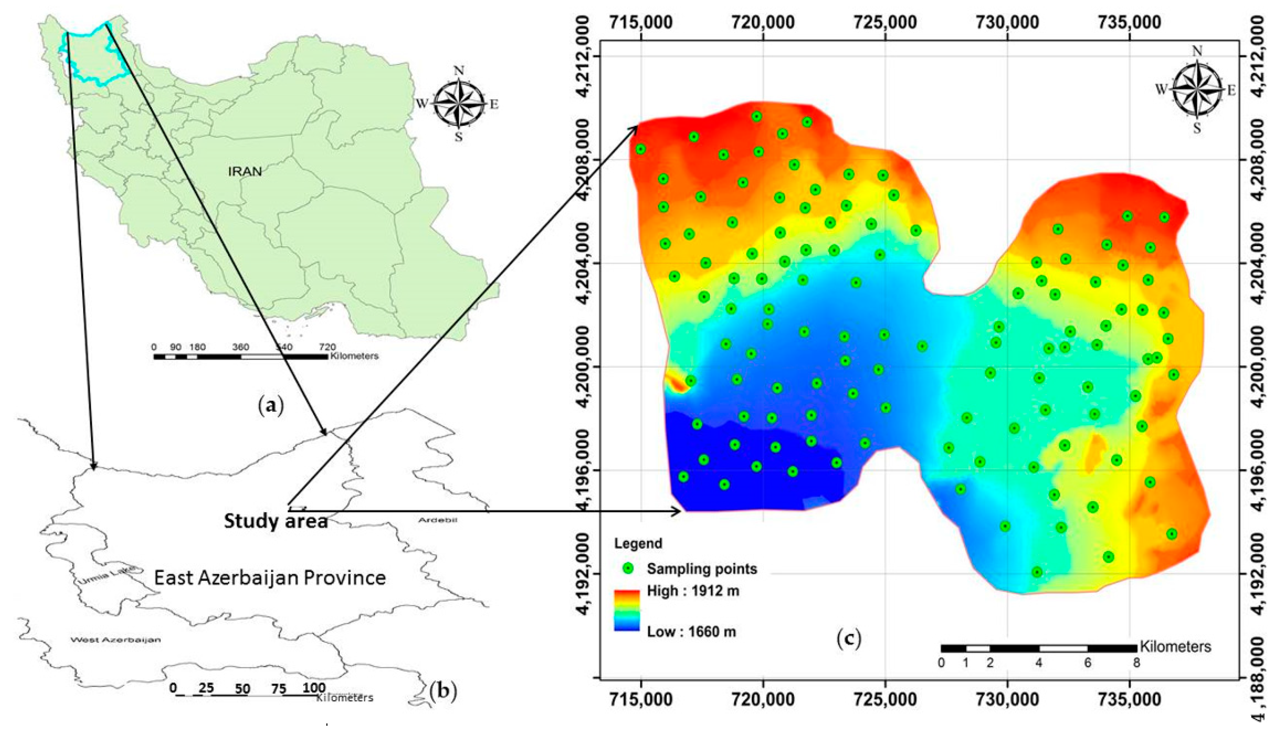
The present study was conducted in the Sarab region in the East Azerbaijan province of Iran, with a total area of 310 km2 and 1660–1912 m altitude (Figure 1). It is located along lat. 37°52′39″ to 38°00′30″ N, long. 47°41′06′′ to 48°26′46″ E (EPSG: 32638). The dominant soil orders for the entire study area were Inceptisols and Entisols [31].

Figure 1.
A brief description of the study area: (a) the map of Iran; (b) the location of the study area in East Azerbaijan province; (c) indication of the sampling points across the study area and the map of digital elevation model (DEM).
Geologically, the low-level piedmont fan and valley terrace deposits comprised about 80% of the study area. The climate is semi-arid with an average annual precipitation of ~280 mm [32]. Field observations revealed that the plant cover was dominated by festuca and alfalfa as perennial plants, and wheat and potato as annual plants. In addition, fallow is not a common practice in this region. The crops mentioned in this study were the crops at the sampling time.
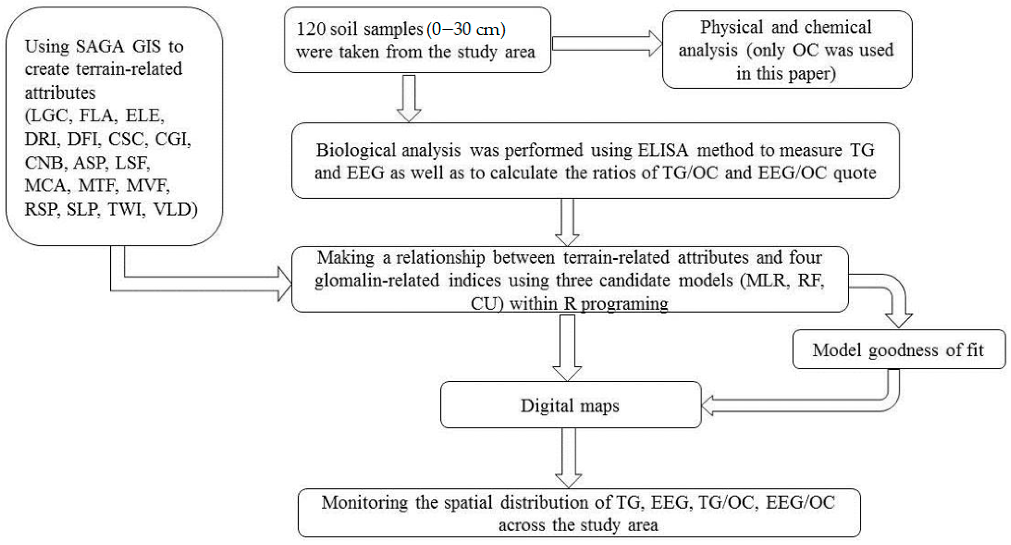
Although sampling designs are very important for validating soil maps [33], in this research, a total of 120 samples were randomly collected in June 2019, covering the whole study area. Since glomalin is mostly found in the A horizon, all soil samples were collected down to 30 cm depth as this is a typical topsoil depth for soils across the study area. The geographical coordinates of the sampling points were carefully navigated in the field using GPS (60CSx, Garmin, Taipei, Taiwan). TG, EEG, and OC were determined in the soil samples as described below. The overall scheme of the procedure is presented in Figure 2.
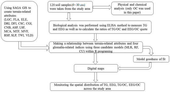
Figure 2.
The general scheme of the procedure used in this experiment. LGC: longitudinal curvature; FLA: flow accumulation; ELE: elevation; DRI: direct insolation; DFI: diffuse insolation; CSC: cross-sectional curvature; CGI: convergence index; CNB: channel network base level; ASP: aspect; LSF: LS factor; MCA: modified catchment area; MTF: multi-resolution ridge top flatness; MVF: multi-resolution index of valley bottom flatness; RSP: relative slope position; SLP: slope; TWI: topographic wetness index; VLD: valley depth; OC: organic carbon; ELISA: enzyme-linked immunosorbent assay; TG: total glomalin; EEG: easily extractable glomalin; MLR: multiple linear regression; RF: random forests; CU: Cubist.
2.2. Soil Analyses
The sampling was performed during three consecutive days. On each day, all collected samples were initially stored in ice boxes (~4 °C) and then immediately transferred to the lab. For glomalin (TG and EEG) determination, nearly 50 g subsamples were kept frozen at −20 °C. The remaining samples were air-dried and sieved through a 10-mesh sieve and kept in room temperature for OC determination.
2.2.1. Determination of Soil Organic Carbon
Soil OC was measured via the method of wet oxidation with chromic acid and back titration with ferrous ammonium sulfate [34].
2.2.2. Glomalin Determination
TG was extracted from soil via autoclaving 1 g of soil in 8 mL of 50 mM sodium citrate with pH 8 at 121 °C for 60 min. After cooling, the extracts were centrifuged at 5000× g for 15 min, and the supernatant was stored at 4 °C for ELISA (enzyme–linked immunosorbent assay) analysis. For EEG determination, the same procedure was used with 20 mM sodium citrate at pH 7 for 30 min of autoclaving [35].
The ELISA method utilizing monoclonal antibody (MAb) 32B11 (Mab32B11) was implemented to determine TG and EEG in the soil extracts. This method is commonly employed for biochemical assays and determines the amount of immunoreactive glomalin. The procedure involved used the MAb32B11 antibody as an initial antibody and biotinylated (horseradish peroxidase–Goat) anti-mouse immunoglobulin M (IgM) antibody as the secondary antibody. MAb32B11 was previously developed from Rhizophagus intraradices FL208 spores that were used to immunize a BALB/c mouse and is specific to glomalin [6].
2.3. DEM-Derived Data
In this research, a total of 17 static covariates (terrain attributes) were created using SAGA GIS software. These attributes were subdivided into four sets of: (a) channels, e.g., channel network base level (CNB) and valley depth (VLD); (b) hydrology, e.g., flow accumulation (FLA), LS factor (LSF), and TWI; (c) lighting visibility, e.g., direct insolation (DRI) and diffuse insolation (DFI); and (d) morphometry, e.g., longitudinal curvature (LGC), elevation (ELE), cross-sectional curvature (CSC), convergence index (CGI), aspect (ASP), modified catchment area (MCA), multi-resolution ridge top flatness (MTF), multi-resolution index of valley bottom flatness (MVF), relative slope position (RSP), and slope (SLP). After creating above-mentioned covariates using SAGA GIS, they were imported to R as predictors. It was obvious that all rasters had same resolution (30-m) and extension (EPSG: 32638). The next step was to stack the imported rasters and point data.
2.4. Modeling with Applications in R
Modeling is commonly used in the general ecological literature to improve the causal understanding developed from observational data [36]. Indeed, R (programming language) version 3.5.1 [37] was used for DSM in this work. Predictive models forecast outputs and estimate metrics. Since the field observations interrelated to TG as well as EEG were not available across the study area, the predictions and digital maps were improved in this study using iterative models of terrain attributes [38]. In this paper, three algorithms, i.e., MLR, RF, and CU, were the candidates for predictions. All three approaches were implemented in the “Caret” package [39].
MLR is one of the simplest approaches to predict values in new locations. In order to fit an MLR model using least squares, the “lm” function (with a total of 17 covariates) was utilized here and a stepwise regression with R was performed to determine statistically significant variables [40]. Implementing this method provided an opportunity to add and remove potential candidates in the models and to keep those with a significant impact on the dependent variables, i.e., glomalin-related indices. RF was also fitted to the dataset using the “randomForest” package in R [41]. One of the advantages of RF is bagging; thus, there was no need for normalization of the dataset. In this paper, to optimize the number of parameters, the number of trees (ntree) and the number of variables or covariates (mtry) were set on 500 and 17, respectively. The former is based upon the mean decrease in accuracy in predictions on the out-of-bag samples, while the latter is a measure of the total decrease in node impurity that results from splits over that variable, averaged over all trees. For plotting the results, the function “varImpPlot” was utilized. The last candidate model used for evaluating was Cubist, which has been implemented in soil science studies [25]. Quinlan [42] reported that the Cubist model can be optimized with three parameters: (a) maximum number of rules or partitions in the data that can be explored; (b) number of committees of boosted iterations of the algorithm, which is similar to the ntree parameter in RF model; (c) extent of allowable extrapolation. To facilitate Cubist model fitting in R, the “Cubist” package was used [43].
2.5. Model Validation
The “goof” function provides a number of model goodness-of-fit measures using the package “ithir” [44]. It includes the root mean square error (RMSE), mean square error (MSE), prediction bias, coefficient of determination (R2), concordance correlation coefficient (CCC) [45], ratio of performance to deviation (RPD), ratio of performance to interquartile distance (RPIQ), and residual variance estimates [40]. Since R2 measures the precision of the relationship between observed and predicted variables, while CCC is a single statistic that both evaluates the accuracy and precision of the relationship, CCC was used as a useful statistic criterion in this research [46]. Therefore, the CCC values were considered to determine the parsimonious model for predicting and digitally mapping the spatial distribution of the studied glomalin-related indices for the entire study area. To distinguish the calculated criteria for either calibration (in-the-bag) or validation (out-of-bag) datasets, the models were set on 200 bags and bootstrapping method was used for iteration [25,47,48].
2.6. Spatial Mapping
DSM has provided a pathway for creating thematic maps to evaluate the spatial distribution of difficult-to-measure properties using easily available ones, e.g., DEM-derived data. To apply the model spatially, the R programming language was deployed to model, manipulate, and map the spatial distribution of TG, EEG, and their ratios on OC due to its high performance in DSM. The application of spatial data analysis in R was well-documented [49,50]. Finally, the results of modeling via R were imported to ArcGIS 10.3 for further visualization. Since in DSM, it is common to create final maps as a stretch mode, the areas with high and low concentrations were only illustrated in this manuscript. However, it could be provided as a classified mode using “Natural Breaks” as default in ArcGIS. As there was no background for separating the classes with maximum differences, the “Natural Breaks” method was used as a default in this study. With this method, class breaks are created, and the method groups similar values together and maximizes the differences between classes. Based on these inputs, maps were then utilized for monitoring and assessing. Although an associated uncertainty map for each created map is useful [40], this was not addressed in this paper. Instead, the optimal model performance from the different goodness-of-fit diagnostics, e.g., R2, RMSE, and CCC, were selected as the parsimonious model. The highest CCC and lowest RMSE were the main criteria.
3. Results
3.1. Soil Data
A brief statistical description of TG, EEG, TG/OC, and EEG/OC is summarized in Table 1.

Table 1.
Summary of the statistical analysis of used field data (n = 120).
Based on the results, TG and EEG showed a fourfold variation between their maximum and minimum values. This variation was also high for TG/OC (24-fold), EEG/OC (39-fold), and OC (47-fold). Normality testing using the Anderson–Darling p–value [51] revealed that EEG was the only normally distributed property among the studied properties. In addition, these results showed that the mean and median were not equivalent for TG, TG/OC, and EEG/OC, indicating the distribution of the data deviated from normality. Therefore, the data for TG was normalized using an inverse normal transformation method. Subsequently, the data for TG/OC and EEG/OC were normalized via the method of log-normal transformation [52]. Both positive and negative skewness with coefficients were determined for the examined properties. The CV of EEG/OC was high, and it was low for EEG. Overall, all studied parameters were categorized as having moderate variability except for EEG/OC based on the classes issued by Fang et al. [53].
3.2. Terrain-Related Attributes
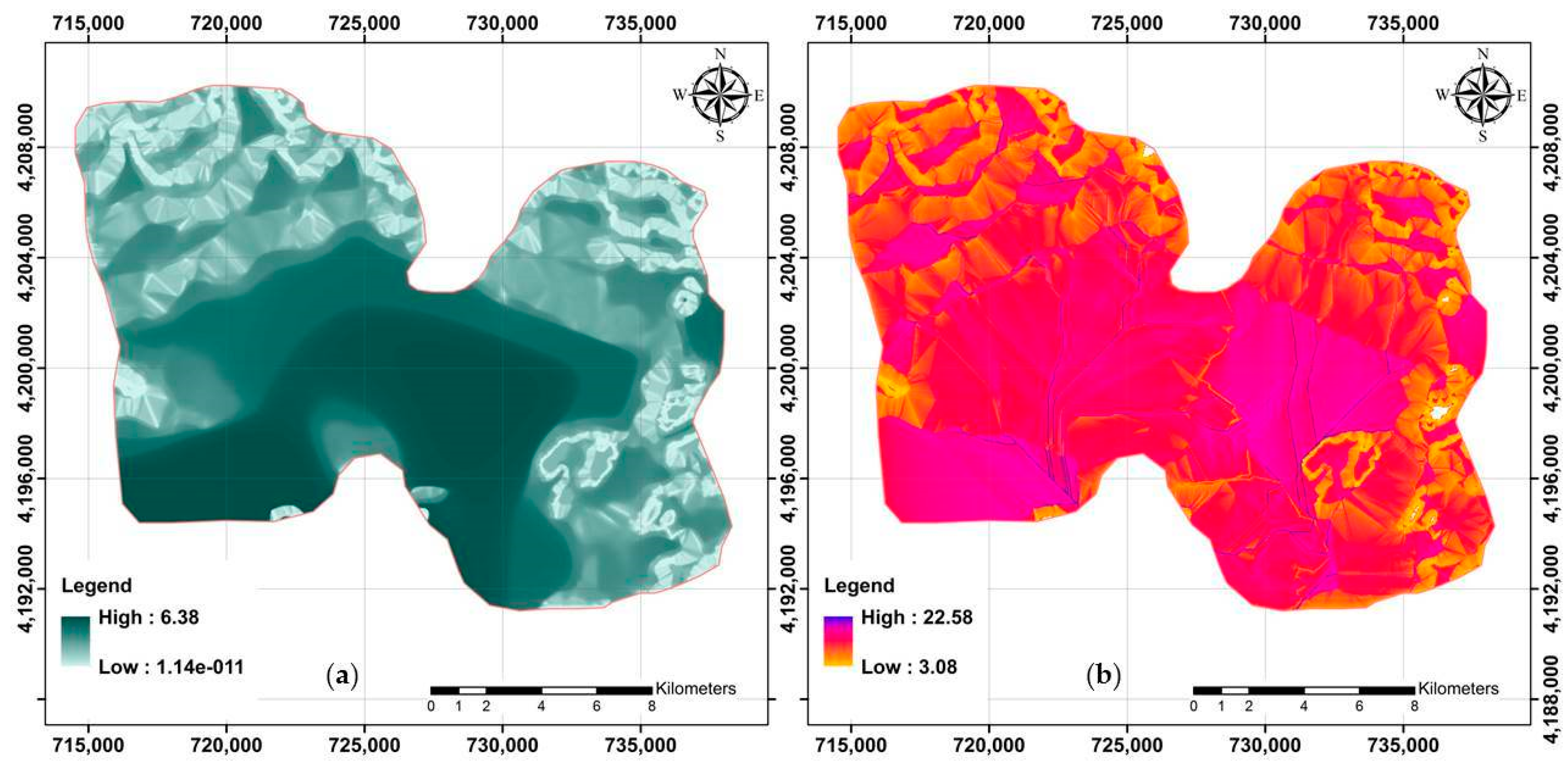
Two DEM derivatives (MVF and TWI) for the study area are presented in Figure 3.

Figure 3.
Two examples of terrain-related attributes applied to model across the study area. (a) MVF (multi-resolution index of valley bottom flatness) and (b) TWI (topographic wetness index).
Summary statistics of these rasters revealed that MVF in the study area varied from 0 to 6.38 (3.58 on average). For further visualization on digital maps, the MVF index was classified into three categories within ArcGIS as follows: (a) Class 1: <2.07; (b) Class 2: 2.07–4.22; and (c) Class 3: 4.22–6.38. Class 3 had an area extension of approximately 42% (located in the central part of the study area), followed by Class 2 (34%) and Class 1 (24%).
In terms of TWI, the results indicated that it varied from 3.08 to 22.58 (11.42 on average) across the study area. In addition, the original map of TWI was categorized into three classes as follows: (a) Class 1: 3.08–9.73; (b) Class 2: 9.73–12.79; and (c) Class 3: 12.79–22.58. This indicated that the vast area included Class 2 (45%), followed by Class 3 (32%) and Class 1 (23%).
Similar rules were performed for the remaining 15 environmental covariates for further analysis for the entire study area. Those are illustrated in Supplementary Material (Figures S1–S15).
3.3. Model Selection
The best fit model among the three candidate algorithms, e.g., MLR, RF, and CU, was selected according to the CCC and RMSE values. The results showed that for the calibration (in the bag), CCC was high compared to the validation (out of the bag) when using all aforementioned algorithms (Table 2). These analyses were based on using the normalized values of the dataset. Based on the findings, MLR and CU were withdrawn from the modeling process due to their lower prediction accuracy in calibration and validation assessments. The overall results demonstrated that RF calibration did not distinctly vary for the four examined properties. However, according to the values of CCC, the best accuracy was found for TG (CCC = 0.33) and EEG (CCC = 0.27) followed by EEG/OC (CCC = 0.24) and TG/OC (CCC = 0.21).
Table 2.
The statistical criteria for evaluating the performance of predictions in calibration and validation datasets across the study area as a result of 200 iterations.
3.4. The Importance of Static Covariates
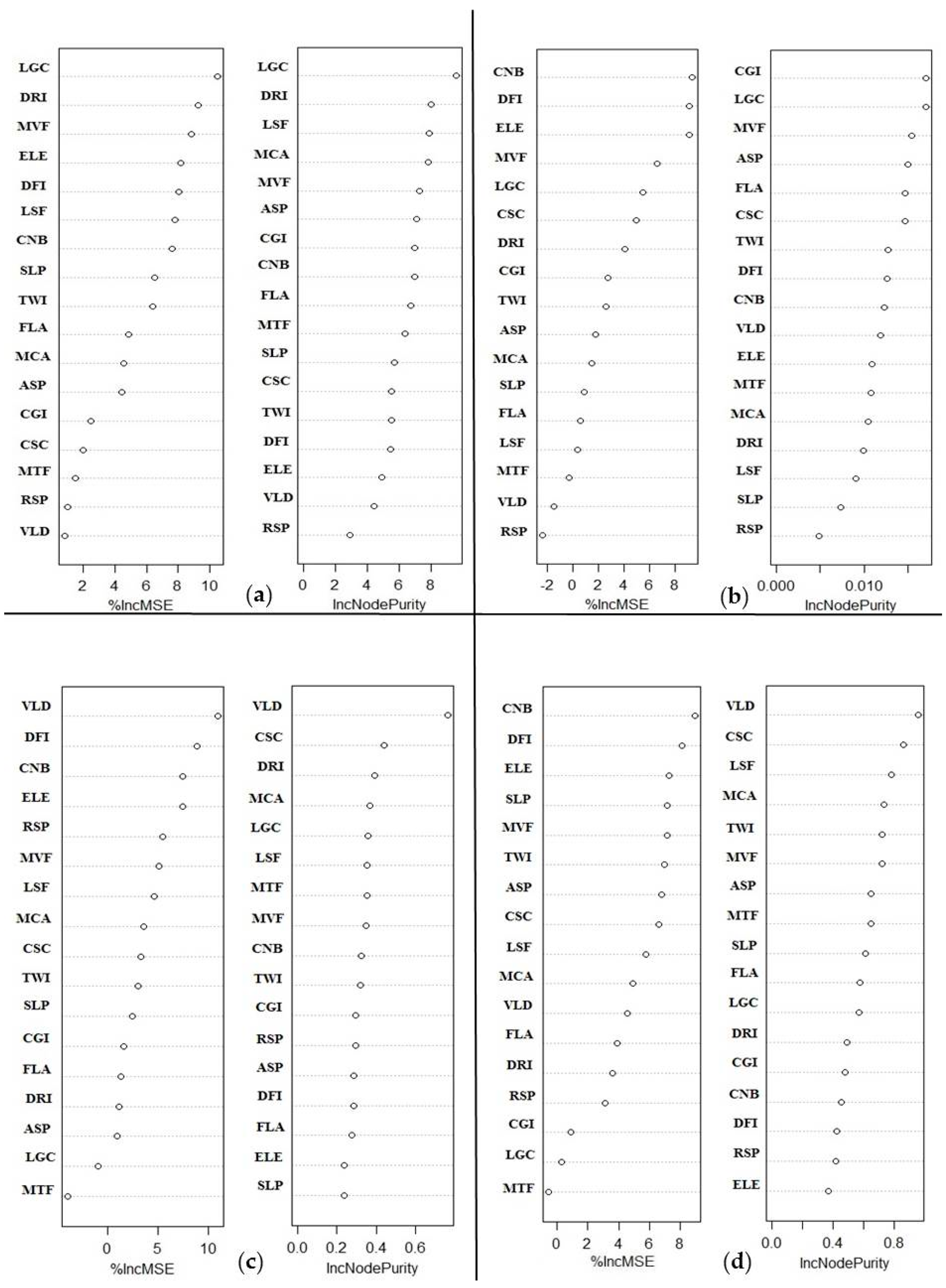
With the application of RF, it is possible to prioritize the importance of covariates in the prediction of glomalin-related indices. It identified a single calculation of importance for each predictor variable that took into account interactions among the 17 DEM-derived attributes without requiring model specification. The covariate importance rankings are illustrated in Figure 4, demonstrating that LGC and VLD were the two most important covariates to predict TG and TG/OC, respectively.
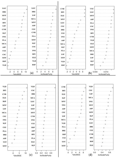
Figure 4.
We used RF model to rank the covariate importance for the studied properties: (a) TG; (b) EEG; (c) TG/OC; and (d) EEG/OC.
3.5. Digital Maps
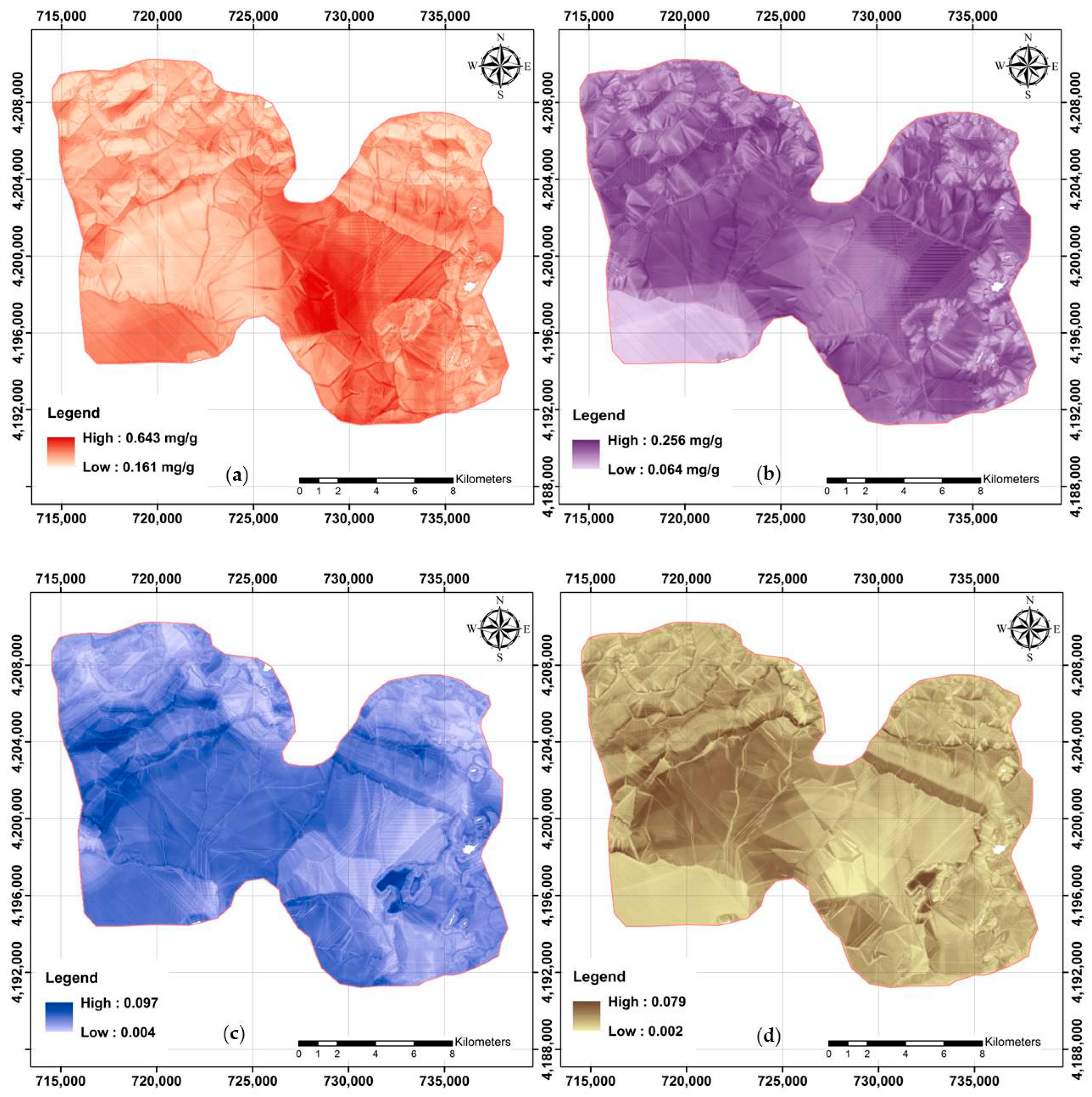
Digital maps were needed prior to digital assessments for each studied soil property. It was also possible to assess the effect of various plant cover types on the distribution pattern of glomalin-related indices across the study area using accurate digital maps. Digital soil maps of TG, EEG, TG/OC, and EEG/OC are shown in Figure 5. The presented values for EEG are based on the original data, while the remaining maps are the back-transformations of the modeled predictions.

Figure 5.
Final digital maps using RF model and available covariates: (a) TG; (b) EEG; (c) TG/OC; and (d) EEG/OC.
Further visualization and analysis were made possible by classifying the maps from raster to vector format [54]. The spatial distribution map of TG was classified into three categories as follows: (a) Class 1: less than 0.271 mg/g; (b) Class 2: 0.271–0.318 mg/g; and (c) Class 3: more than 0.318 mg/g. Class 2 had an area extension of approximately 41%, followed by Class 1 (38%) and Class 3 (21%). The mean value of TG, 0.29 mg/g, based on RF analyses for the study area was close to the measured mean value. However, TG varied widely across the study area (0.161–0.643 mg/g).
Approximately 46%, 39%, and 15% of the study area was classified into three EEG classes as follows: (a) Class 3 (more than 0.168 mg/g), Class 2 (0.141–0.168 mg/g), and Class 1 (less than 0.141 mg/g), respectively. The mean value of both the predicted pixel values and the original measured data were not significantly different and reflected the accuracy of the modeling.
4. Discussion
4.1. Plant Cover Type Effects on Soil Glomalin
One of the advantages of DSM is to find an opportunity for investigating soil–landscape relationships. To monitor plant cover type effects, the cells of a raster based on a set of coordinate points comprising various covers were extracted and indicated that annual crops and perennial plants had different impacts on TG, EEG, TG/OC, and EEG/OC. In general, TG results from the accumulation of glomalin in soil over years of cultivation, while EEG is the recently produced glomalin. Therefore, the recalcitrant C source of the soil showed a variety of differences among anthropogenic management activities in the study area. Since the soil in perennial plants is not disturbed and is not subjected to tillage every year, the mycorrhizal network structure remains intact and active for the continued secretion of glomalin. Yearly tillage for the cultivation of annual crops reduces the active AM fungal populations. In summary, the study showed that the prediction of soil glomalin using easily measured variables helps to manage and monitor natural grasslands and cultivated areas in a manner that encourages mycorrhizal network development and improves glomalin production. Compared to annual crops, perennials showed the highest influence on carbon sequestration in terms of glomalin production. This means that tillage practices are the most important factor for conserving the C pool in soil. Moreover, accelerated tillage practices decrease OC as well as its mean residence time in soil [55].
As was expected, the highest values of TG were associated with the undisturbed areas (grasslands dominated by festuca), and the lowest values were found in the cultivated areas. Therefore, TG must have been higher than EEG because, based on the field observations, the vast study area was covered by perennial plants, i.e., festuca and alfalfa. A similar observation showed that TG in a forest ecosystem of the temperate Himalayan region is approximately two times more than that of a wheat field [56]. The differences between TG and EEG in soils of perennial plants, including festuca and alfalfa, were greater than those between soils of annual crops, i.e., wheat and potato. Despite having high TG in alfalfa, its EEG was lower compared to the other plants. This can be explained by the tripartite symbiosis of alfalfa–mycorrhizal fungi–rhizobia as the carbon allocated to the alfalfa root is divided between the bacterial and fungal microsymbionts [57].
The highest OC being in soils dominated by festucas can be attributed to the absence of tillage in grassland conditions. The loss of carbon from agricultural soils is strongly associated with tillage severity [58]. Carbon constitutes about 50% of the glomalin molecule, representing, in turn, 0.52–1.62% of the soil OC pool. Many scientists previously reported that soil OC can be successfully predicted with DEM-derived data not only in semi-arid regions [59] but also in permafrost regimes [60]. A positive correlation between soil OC and TG or EEG was found, which re-iterated their contributions to the soil carbon pool, and the relation of soil glomalin content with plant cover types and its applicability as a putative indicator of carbon sequestration has been reported previously [61]. The low values for TG/OC and EEG/OC ratios in festucas can be understood by considering the huge amount of OC in this plant type, despite the relatively higher TG and EEG.
4.2. The Role of DEM-Derived Data
The most important finding of this study was that the terrain-related attributes successfully contributed to the modeling and mapping of recalcitrant C sources of soils in the study area. The performance of DEM-derived data as a subset of digital soil morphometrics was described by Hartemink and Minasny [62]. It was also reported that latitude and longitude, in addition to soil OC and total nitrogen, can be a useful predictor to estimate the distribution of the fungal community [30]. The importance of terrain-related attributes may be explained by the idea that soil OC can be estimated with topographic properties [63]. Notwithstanding that remotely sensed data did not contribute to the prediction of glomalin-related indices, the relationship between NDVI with DEM was previously reported [64]. Moreover, the possibilities for the application of DEM for mapping vegetation tiers have been explored [65]. Since there is a strong correlation between soil OC and TG or EEG [66], the spatial distribution of TG, EEG, TG/OC, and EEG/OC was successfully predicted by using only terrain-related attributes, as was expected.
4.3. Accuracy of Modeling and Covariates Ranking
Among the three candidate models, RF outperformed MLR and CU with the chosen soil data and static environmental covariates in the present study. Belgiu and Drăguţ [67] pointed out that RF has become popular within pedometrics due to the accuracy of its classifications. Although the validation was not high, it was considered because the terrain-related attributes, as easy-to-measure static environmental covariates, were divergent from the target variable. A similar conflict was reported in terms of OC. The efficiency of RF for predicting soil OC (and glomalin) has been previously reported [13], but Were et al. [68] reported a high tendency for overestimations. Moreover, the greatest accuracy was found for the prediction of TG followed by EEG, EEG/OC, and TG/OC.
LGC and VLD were identified as the two most important covariates to predict TG and TG/OC, respectively. Furthermore, CNB was recognized as the most important covariate to predict both EEG and EEG/OC. The other crucial covariates for predicting all studied properties were DRI and DFI, which were classified into the lightening visibility category. Since the production of glomalin by fungi highly depends on their successful symbiosis with plant roots and sufficient photosynthates, radiation played an important role, as was expected. Among the 17 studied covariates, the MVF and ELE in the RF model for the prediction of all parameters were identified in the subsequent importance ranking. The importance of the MVF index for identifying valley bottoms from hill slopes to distinguish sediment deposits was also reported by Gallant and Dowling [69]. TWI has also proven to be a significant indicator in explaining soil moisture and OC status [70]. Moreover, Pei et al. [28] reported that OC can be predicted by TWI, although it only played a moderate role in this research. The overall outcomes showed that the importance of variables differed for each studied property.
4.4. Digital Assessments
The final step was the digital soil assessment [12] to understand the spatial distribution of soil glomalin across the study area. The application of DSM is useful to evaluate the spatial distribution of glomalin-related indices and involves easily measured parameters. Although four sets of DEM-derived data (e.g., channels; hydrology; lighting; and morphometry) were used in the modeling process, the intensity of lighting visibility and radiation, viz., DFI and DRI, played a crucial role in the digital mapping of soil glomalin. A possible reason for this is that the production of glomalin by fungi highly depends on their successful symbiosis with plant roots and creating enough photosynthates.
Digital TG and EEG maps, as a result of RF modeling, identified locations of high and low concentrations in the entire study area. For example, the highest value of TG was found in the central part and somewhat south of the study area, which was mainly covered by festuca and alfalfa. This can be attributed to the fact that those areas have a moderate catchment area and high TWI. Further visualization using the aforementioned digital maps showed that the spatial distribution of EEG did not correspond to TG variation across the study area, which was most likely due to the different natures of cultivated and grassland plant species along with their different field practices. Integrated assessments of field observations and digital maps revealed that potato and wheat, as annual crops, were the most frequent plant cover in the area containing high EEG. Since EEG represents newly formed glomalin, its abundance was seen in potato and wheat cultivated areas.
The fluctuation in the TG/OC ratio in the study area was almost the same as that observed for the EEG/OC ratio; this may be due to their dependence on both glomalin and soil OC content. TG/OC and EEG/OC represent the glomalin–C quote of soil OC. These seem to be very important indicators for explaining carbon conservation in soil. Therefore, the spatial distribution maps of the above-mentioned ratios (Figure 5c,d) were provided previously for detailed illustrations. Since soil glomalin content, as a recalcitrant C source, has a positive correlation with soil OC, it could be an effective indicator, in part, to monitor soil carbon sequestration. Consequently, it would be possible to enrich soil C pools with low-degrading C compounds and increase carbon sequestration as well. Festuca had the highest influence on carbon sequestration via glomalin production, followed by alfalfa, potato, and wheat. This can be explained by the fact that forage crops without tillage sequester carbon by declining CO2 emissions and maintaining the mycorrhizal network. Moreover, this effect is vital to mitigate environmental challenges such as climate change.
5. Conclusions
Since soil glomalin content, as a recalcitrant C source, showed a significantly positive correlation with soil OC, it could be an effective indicator to monitor soil carbon sequestration. Our findings showed that terrain-related attributes can predict the spatial distribution of TG, EEG, and their ratios on OC successfully. Since the production of glomalin by fungi highly depends on their successful symbiosis with plant roots and receiving enough photosynthates, as we expected, the intensity of lighting visibility, e.g., DFI and DRI, played a crucial role on the digital mapping of soil glomalin.
Based on the findings, RF outperformed MLR and CU using available field soil data and environmental covariates. Moreover, the most accuracy was found for the prediction of EEG followed by EEG/OC, TG, and TG/OC. In general, this article revealed that DSM plays an important role in soil biological traits. For instance, it can assist us with managing natural grasslands and monitoring climate change impacts.
Our findings showed that terrain-related attributes could be successfully used in predicting glomalin-related indices. Since this paper outlines the performance of DSM and terrain-related attributes, it is advisable to further investigate this scenario using remote sensing data, e.g., Landsat 8 OLI, Sentinel, MODIS, etc.
Supplementary Materials
The following supporting information can be downloaded at: https://www.mdpi.com/article/10.3390/agronomy12071653/s1, Figure S1: The stretched map relevant to aspect (ASP); Figure S2: The stretched map relevant to convergence index (CGI); Figure S3: The stretched map relevant to channel network base level (CNB); Figure S4: The stretched map relevant to cross-sectional curvature (CSC); Figure S5: The stretched map relevant to diffuse insolation (DFI); Figure S6: The stretched map relevant to direct insolation (DRI); Figure S7: The stretched map relevant to elevation (ELE); Figure S8: The stretched map relevant to flow accumulation (FLA); Figure S9: The stretched map relevant to longitudinal curvature (LGC); Figure S10: The stretched map relevant to LS factor (LSF); Figure S11: The stretched map relevant to modified catchment area (MCA); Figure S12: The stretched map relevant to multi-resolution ridge top flatness (MTF); Figure S13: The stretched map relevant to relative slope position (RSP); Figure S14: The stretched map relevant to slope (SLP); Figure S15: The stretched map relevant to valley depth (VLD).
Author Contributions
Conceptualization, N.A. and F.S.; methodology, N.A. and L.A.M.; software, A.S., F.S., and A.B.; validation, F.S. and N.A.; formal analysis, A.S., N.N., and L.A.M.; investigation, A.S.; resources, F.S. and A.B.; data curation, N.A. and A.S.; writing—original draft preparation, A.S.; writing—review and editing, A.B.; visualization, F.S.; supervision, N.A. and L.A.M.; project administration, N.A.; funding acquisition, N.A. All authors have read and agreed to the published version of the manuscript.
Funding
The APC was paid from the Natural Sciences and Engineering Research Council Grant #RGPIN-2014-04100 and was received by A.B.
Data Availability Statement
Not applicable.
Acknowledgments
The authors would like to thank the University of Tabriz for providing lab facilities. In addition, the immunoassay of glomalin was performed by the Immunology Research Center of the Tabriz University of Medical Sciences, which we are grateful for.
Conflicts of Interest
The authors declare no conflict of interest.
References
- Vlček, V.; Pohanka, M. Glomalin—An interesting protein part of the soil organic matter. Soil Water Res. 2020, 15, 67–74. [Google Scholar] [CrossRef]
- Nichols, K.A.; Wright, S.F. Carbon and nitrogen in operationally defined soil organic matter pools. Biol. Fert. Soils 2006, 43, 215–220. [Google Scholar] [CrossRef]
- Lal, R. Soil carbon sequestration to mitigate climate change. Geoderma 2004, 123, 1–22. [Google Scholar] [CrossRef]
- Barna, G.; Makó, A.; Takács, T.; Skic, K.; Füzy, A.; Horel, A. Biochar alters soil physical characteristics, arbuscular mycorrhizal fungi colonization, and glomalin production. Agronomy 2020, 10, 1933. [Google Scholar] [CrossRef]
- Walley, F.L.; Gillespie, A.W.; Adetona, A.B.; Germida, J.J.; Farrell, R.E. Manipulation of rhizosphere organisms to enhance glomalin production and C sequestration: Pitfalls and promises. Can. J. Plant. Sci. 2013, 94, 1025–1032. [Google Scholar] [CrossRef]
- Wright, S.F.; Franke-Snyder, M.; Morton, J.B.; Upadhyaya, A. Time-course study and partial characterization of a protein on hyphae of arbuscular mycorrhizal fungi during active colonization of roots. Plant. Soil 1996, 181, 193–203. [Google Scholar] [CrossRef]
- Zeraatpisheh, M.; Jafari, A.; Bagheri Bodaghabadi, M.; Ayoubi, S.; Taghizadeh–Mehrjardi, R.; Toomanian, N.; Kerry, R.; Xu, M. Conventional and digital soil mapping in Iran: Past, present, and future. Catena 2020, 188, e104424. [Google Scholar] [CrossRef]
- McBratney, A.B.; Santos, M.M.; Minasny, B. On digital soil mapping. Geoderma 2003, 117, 3–52. [Google Scholar] [CrossRef]
- Arrouays, D.; Lagacherie, P.; Hartemink, A.E. Digital soil mapping across the globe. Geoderma Reg. 2017, 9, 1–4. [Google Scholar] [CrossRef]
- Ma, X.; Minasny, B.; Malone, B.P.; McBratney, A.B. Pedology and digital soil mapping (DSM). Eur. J. Soil Sci. 2019, 70, 216–235. [Google Scholar] [CrossRef]
- Cámara, J.; Gómez–Miguel, V.; Martín, M.Á. Lithologic control on soil texture heterogeneity. Geoderma 2017, 287, 157–163. [Google Scholar] [CrossRef]
- Carré, F.; McBratney, A.B.; Mayr, T.; Montanarella, L. Digital soil assessments: Beyond DSM. Geoderma 2007, 142, 69–79. [Google Scholar] [CrossRef]
- Taghizadeh–Mehrjardi, R.; Nabiollahi, K.; Kerry, R. Digital mapping of soil organic carbon at multiple depths using different data mining techniques in Baneh region, Iran. Geoderma 2016, 266, 98–110. [Google Scholar] [CrossRef]
- Sindayihebura, A.; Ottoy, S.; Dondeyne, S.; van Meirvenne, M.; van Orshoven, J. Comparing digital soil mapping techniques for organic carbon and clay content: Case study in Burundi’s central plateaus. Catena 2017, 156, 161–175. [Google Scholar] [CrossRef]
- Wang, S.; Jin, X.; Adhikari, K.; Li, W.; Yu, M.; Bian, Z.; Wang, Q. Mapping total soil nitrogen from a site in northeastern China. Catena 2018, 166, 134–146. [Google Scholar] [CrossRef]
- Mousavi, A.; Shahbazi, F.; Oustan, S.; Jafarzadeh, A.A.; Minasny, B. Spatial distribution of iron forms and features in the dried lake bed of Urmia Lake of Iran. Geoderma Reg. 2020, 21, e00275. [Google Scholar] [CrossRef]
- López-Castañeda, A.; Zavala-Cruz, J.; Palma-López, D.J.; Rincón-Ramírez, J.A.; Bautista, F. Digital mapping of soil profile properties for precision agriculture in developing countries. Agronomy 2022, 12, 353. [Google Scholar] [CrossRef]
- Minasny, B.; McBratney, A.B.; Mendonça Santos, M.; Odeh, I.; Guyon, B. Prediction and digital mapping of soil carbon storage in the Lower Namoi Valley. Aust. J. Soil Res. 2006, 44, 233–244. [Google Scholar] [CrossRef]
- Fathololoumi, S.; Vaezi, A.R.; Alavipanah, S.K.; Ghorbani, A.; Saurette, D.; Biswas, A. Improved digital soil mapping with multitemporal remotely sensed satellite data fusion: A case study in Iran. Sci. Total Environ. 2020, 721, e137703. [Google Scholar] [CrossRef]
- Schwalb-Willmann, J.; Remelgado, R.; Safi, K.; Wegmann, M. MOVEVIS: Animating movement trajectories in synchronicity with static or temporally dynamic environmental data in R. Methods Ecol. Evol. 2020, 11, 664–669. [Google Scholar] [CrossRef] [Green Version]
- Peng, J.; Biswas, A.; Jiang, Q.; Zhao, R.; Hu, J.; Hu, B.; Shi, Z. Estimating soil salinity from remote sensing and terrain data in southern Xinjiang Province, China. Geoderma 2019, 337, 1309–1319. [Google Scholar] [CrossRef]
- Bagheri Bodaghabadi, M.; Martínez–casasnovas, J.A.; Salehi, M.H.; Mohammadi, J.; Esfandiarpoor Borujeni, I.; Toomanian, N.; Gandomkar, A. Digital soil mapping using artificial neural networks and terrain–related attributes. Pedosphere 2015, 25, 580–591. [Google Scholar] [CrossRef] [Green Version]
- Hengl, T.; Heuvelink, G.B.M.; Kempen, B.; Leenaars, J.G.B.; Walsh, M.G.; Shepherd, K.D.; Sila, A.; MacMillan, R.A.; de Jesus, J.M.; Tamene, L.; et al. Mapping soil properties of Africa at 250 m resolution: Random forests significantly improve current predictions. PLoS ONE 2015, 10, e0125814. [Google Scholar] [CrossRef]
- Behrens, T.; Forster, H.; Scholten, T.; Steinrucken, U.; Spies, E.D.; Goldschmitt, M. Digital soil mapping using artificial neural network. J. Plant. Nutr. Soil Sci. 2005, 168, 21–33. [Google Scholar] [CrossRef]
- Shahbazi, F.; Hughes, P.; McBratney, A.B.; Minasny, B.; Malone, B.P. Evaluating the spatial and vertical distribution of agriculturally important nutrients—Nitrogen, phosphorous and boron—In North West Iran. Catena 2019, 173, 71–82. [Google Scholar] [CrossRef]
- Luoto, M.; Hjort, J. Evaluation of current statistical approaches for predictive geomorphological mapping. Geomorphology 2005, 67, 299–315. [Google Scholar] [CrossRef]
- Meier, M.; de Souza, E.; Francelino, M.R.; Fernandes Filho, E.I.; Schaefer, C.E.G.R. Digital soil mapping using machine learning algorithms in a tropical mountainous area. Rev. Bras. Cienc. Solo 2018, 42, e0170421. [Google Scholar] [CrossRef] [Green Version]
- Pei, T.; Qin, C.Z.; Zhu, A.X.; Yang, L.; Luo, M.; Li, B.; Zhou, C. Mapping soil organic matter using the topographic wetness index: A comparative study based on different flow–direction algorithms and kriging methods. Ecol. Indic. 2010, 10, 610–619. [Google Scholar] [CrossRef]
- Staunton, S.; Nicolas, P.A.; Saby, N.; Arrouays, D.; Quiquampoix, H. Can soil properties and land use explain glomalin–related soil protein (GRSP) accumulation? A nationwide survey in France. Catena 2020, 193, e104620. [Google Scholar] [CrossRef]
- Chen, Y.; Xu, T.; Fu, W.; Hu, Y.; Hu, L. Soil organic carbon and total nitrogen predict large–scale distribution of soil fungal communities in temperate and alpine shrub ecosystems. Eur. J. Soil Biol. 2021, 102, e103270. [Google Scholar] [CrossRef]
- USDA. Keys to Soil Taxonomy, 12th ed.; Soil Survey Staff: Washington, DC, USA, 2014. [Google Scholar]
- IRIMO. Islamic Republic of Iran Meteorological Organization: Tehran, Iran. 2012. Available online: https://irandataportal.syr.edu/iran-meteorological-organization (accessed on 23 April 2022).
- Biswas, A.; Zhang, Y. Sampling designs for validating digital soil maps: A review. Pedosphere 2018, 28, 1–15. [Google Scholar] [CrossRef]
- Nelson, D.W.; Sommers, L.E. Total carbon, organic carbon, and organic matter. In Methods of Soil Analysis: Part 3, Chemical Methods, 5.3; Sparks, D.L., Page, A.L., Helmke, P.A., Loeppert, R.H., Soltanpour, P.N., Tabatabai, M.A., Johnston, C.T., Sumner, M.E., Eds.; American Society of Agronomy: Madison, WI, USA, 1996. [Google Scholar] [CrossRef]
- Wright, S.F.; Upadhyaya, A. Extraction of AN abundant and unusual protein from soil and comparison with hyphal protein from arbuscular mycorrhizal fungi. Soil Sci. 1996, 161, 575–586. [Google Scholar] [CrossRef]
- Eisenhauer, N.; Bowker, M.A.; Grace, J.B.; Powell, J.R. From patterns to causal understanding: Structural equation modeling (SEM) in soil ecology. Pedobiologia 2015, 58, 65–72. [Google Scholar] [CrossRef] [Green Version]
- R Core Team. R: A Language and Environment for Statistical Computing; R Foundation for Statistical Computing: Vienna, Austria, 2017; Available online: https://www.R-project.org/ (accessed on 23 April 2022).
- Hengl, T.; McMillan, R.A. Predictive Soil Mapping with R; OpenGeoHub Foundation: Wageningen, The Netherlands, 2019; ISBN 978-0-359-30635-0. [Google Scholar]
- Kuhn, M.; Weston, S.; Keefer, C.; Coulter, N. C Code for Cubist. Cubist: Rule– and Instance–Based Regression Modeling. 2016. Available online: https://CRAN.R–project.org/package=Cubist (accessed on 23 April 2022).
- Malone, B.P.; Minasny, B.; McBratney, A.B. Using R for Digital Soil Mapping; Springer: Berlin/Heidelberg, Germany, 2017. [Google Scholar] [CrossRef]
- Liaw, A.; Wiener, M. Classification and Regression by Random Forest. R News 2002, 2, 18–22. [Google Scholar]
- Quinlan, J.R. Learning with continuous classes. In Proceedings of the AI92, 5th Australian Conference on Artificial Intelligence, Hobart, Tasmania, 16–18 November 1992; World Scientific: Singapore, 1992; pp. 343–348. [Google Scholar]
- Kuhn, M.; Quinlan, R. Cubist: Rule– And Instance–Based Regression Modeling. R Package Version 0.2.2. 2018. Available online: https://CRAN.R–project.org/package=Cubist (accessed on 23 April 2022).
- Malone, B.P. ithir: Functions and Algorithms Specific to Pedometrics. R Package Version 1.0/r126. 2016. Available online: https://R-Forge.R-project.org/projects/ithir/ (accessed on 23 April 2022).
- Lin, L.I. A concordance correlation coefficient to evaluate reproducibility. Biometrics 1989, 45, 255–268. [Google Scholar] [CrossRef]
- Bellon-Maurel, V.; Fernandez-Ahumada, E.; Palagos, B.; Roger, J.-M.; McBratney, A.B. Critical review of chemometric indicators commonly used for assessing the quality of the prediction of soil attributes by NIR spectroscopy. TrAC Trends Anal. Chem. 2010, 29, 1073–1081. [Google Scholar] [CrossRef]
- Ma, Y.; Minasny, B.; Wu, C. Mapping key soil properties to support agricultural production in Eastern China. Geoderma Reg. 2017, 10, 144–153. [Google Scholar] [CrossRef]
- Shahbazi, F.; McBratney, A.B.; Malone, B.P.; Oustan, S.; Minasny, B. Retrospective monitoring of the spatial variability of crystalline iron in soils of the east shore of Urmia Lake, Iran using remotely sensed data and digital maps. Geoderma 2019, 337, 1196–1207. [Google Scholar] [CrossRef]
- Bivand, R.S.; Pebesma, E.J.; Gomez–Rubio, V. Applied Spatial Data Analysis with R, 2nd ed.; Springer: New York, NY, USA, 2008. [Google Scholar] [CrossRef]
- Heuvelink, G.B.M. Uncertainty and uncertainty propagation in soil mapping and modelling. In Pedometrics; McBratney, A.B., Minasny, B., Stockmann, U., Eds.; Springer: Cham, Switzerland, 2018; pp. 439–461. [Google Scholar] [CrossRef]
- Anderson, T.W.; Darling, D.A. Asymptotic theory of certain “goodness of fit” criteria based on stochastic processes. Ann. Math. Statist. 1952, 23, 193–212. [Google Scholar] [CrossRef]
- Landau, S.; Everitt, B.S. A Handbook of Statistical Analyses Using SPSS; Chapman & Hall/CRC Press: Boca Raton, FL, USA, 2004. [Google Scholar]
- Fang, X.; Xue, Z.; Li, B.; An, S. Soil organic carbon distribution in relation to land use and its storage in a small watershed of the Loess Plateau, China. Catena 2012, 88, 6–13. [Google Scholar] [CrossRef]
- Ayhan, E.; Akar, O.; Uzun, S.; Dilavar, A.; Kansu, O. Analysis of digital data obtained from raster and vector maps. J. Surv. Eng. 2010, 137, 65–69. [Google Scholar] [CrossRef]
- Rahmati, M.; Eskandari, I.; Kouselou, M.; Feiziasl, V.V.; Mahdavinia, G.R.; Aliasgharzad, N.; McKenzie, B.M. Changes in soil organic carbon fractions and residence time five years after implementing conventional and conservation tillage practices. Soil Till. Res. 2020, 200, e104632. [Google Scholar] [CrossRef]
- Nautiyal, P.; Rajput, R.; Pandey, D.; Arunachalam, K.; Arunachalam, A. Role of glomalin in soil carbon storage and its variation across land uses in temperate Himalayan regime. Biocatal. Agric. Biotechnol. 2019, 21, e101311. [Google Scholar] [CrossRef]
- Kafle, A.; Garcia, K.; Wang, X.; Pfeffer, P.E.; Strahan, G.D.; Bücking, H. Nutrient demand and fungal access to resources control the carbon allocation to the symbiotic partners in tripartite interactions of Medicago truncatula. Plant. Cell Environ. 2018, 42, 270–284. [Google Scholar] [CrossRef] [Green Version]
- Haddaway, N.R.; Hedlund, K.; Jackson, L.E.; Katterer, T.; Lugato, E.; Thomsen, I.K.; Jørgensen, H.B.; Isberg, P.E. How does tillage intensity affect soil organic carbon? A systematic review. Environ. Evid. 2017, 6, 30. [Google Scholar] [CrossRef] [Green Version]
- Mondal, A.; Khare, D.; Kundu, S.; Mondal, S.; Mukherjee, S.; Mukhopadhyay, A. Spatial soil organic carbon (SOC) prediction by regression kriging using remote sensing data. Egypt. J. Remote Sens. Space Sci. 2017, 20, 61–70. [Google Scholar] [CrossRef] [Green Version]
- Weiss, N.; Faucherre, S.; Lampiris, N.; Wojcik, R. Elevation–based upscaling of organic carbon stocks in High–Arctic permafrost terrain: A storage and distribution assessment for Spitsbergen, Svalbard. Polar Res. 2017, 36, e1400363. [Google Scholar] [CrossRef]
- Hammer, E.; Rillig, M.C. The influence of different stresses on glomalin levels in an Arbuscular Mycorrhizal fungus—salinity increases glomalin content. PLoS ONE 2011, 6, e28426. [Google Scholar] [CrossRef] [Green Version]
- Hartemink, A.E.; Minasny, B. Developments in digital soil morphometrics. In Digital Soil Morphometrics; Hartemink, A., McBratney, A.B., Eds.; Springer: Berlin/Heidelberg, Germany, 2016; pp. 425–433. [Google Scholar]
- She, D.; Xuemei, G.; Jingru, S.; Timm, L.C.; Hu, W. Soil organic carbon estimation with topographic properties in artificial grassland using a state-space modeling approach. Can. J. Soil Sci. 2014, 94, 503–514. [Google Scholar] [CrossRef]
- Miao, L.; Jiang, C.; Xue, B.; Liu, Q.; He, B.; Nath, R.; Cui, X. Vegetation dynamics and factor analysis in arid and semi–arid Inner Mongolia. Environ. Earth Sci. 2015, 73, 2343–2352. [Google Scholar] [CrossRef]
- Volařík, D. Application of digital elevation model for mapping vegetation tiers. J. For. Sci. 2010, 56, 112–120. [Google Scholar] [CrossRef] [Green Version]
- Tian, Y.; Yan, C.; Wang, Q.; Ma, W.; Yang, D.; Liu, J.; Lu, H. Glomalin–related soil protein enriched in δ13 C and δ15 N excels at storing blue carbon in mangrove wetlands. Sci. Total Environ. 2010, 732, e138327. [Google Scholar] [CrossRef]
- Belgiu, M.; Drăguţ, L. Random forest in remote sensing: A review of applications and future directions. ISPRS J. Photogramm. Remote Sens. 2016, 114, 24–31. [Google Scholar] [CrossRef]
- Were, K.; Bui, D.T.; Dick, Ø.B.; Singh, B.R. A comparative assessment of support vector regression, artificial neural networks, and random forests for predicting and mapping soil organic carbon stocks across an Afromontane landscape. Ecol. Indic. 2015, 52, 394–403. [Google Scholar] [CrossRef]
- Gallant, J.C.; Dowling, T.I. A multiresolution index of valley bottom flatness for mapping depositional areas. Water Resour. Res. 2003, 39, 1347–1359. [Google Scholar] [CrossRef]
- Raduła, M.W.; Szymura, T.H.; Szymura, M. Topographic wetness index explains soil moisture better than bioindication with Ellenberg’s indicator values. Ecol. Indic. 2018, 85, 172–179. [Google Scholar] [CrossRef]
Publisher’s Note: MDPI stays neutral with regard to jurisdictional claims in published maps and institutional affiliations. |
© 2022 by the authors. Licensee MDPI, Basel, Switzerland. This article is an open access article distributed under the terms and conditions of the Creative Commons Attribution (CC BY) license (https://creativecommons.org/licenses/by/4.0/).