
VICAL: Global Calculator to Estimate Vegetation Indices for Agricultural Areas with Landsat and Sentinel-2 Data

 ,
,  , , and
Abstract
:1. Introduction
2. Materials and Methods
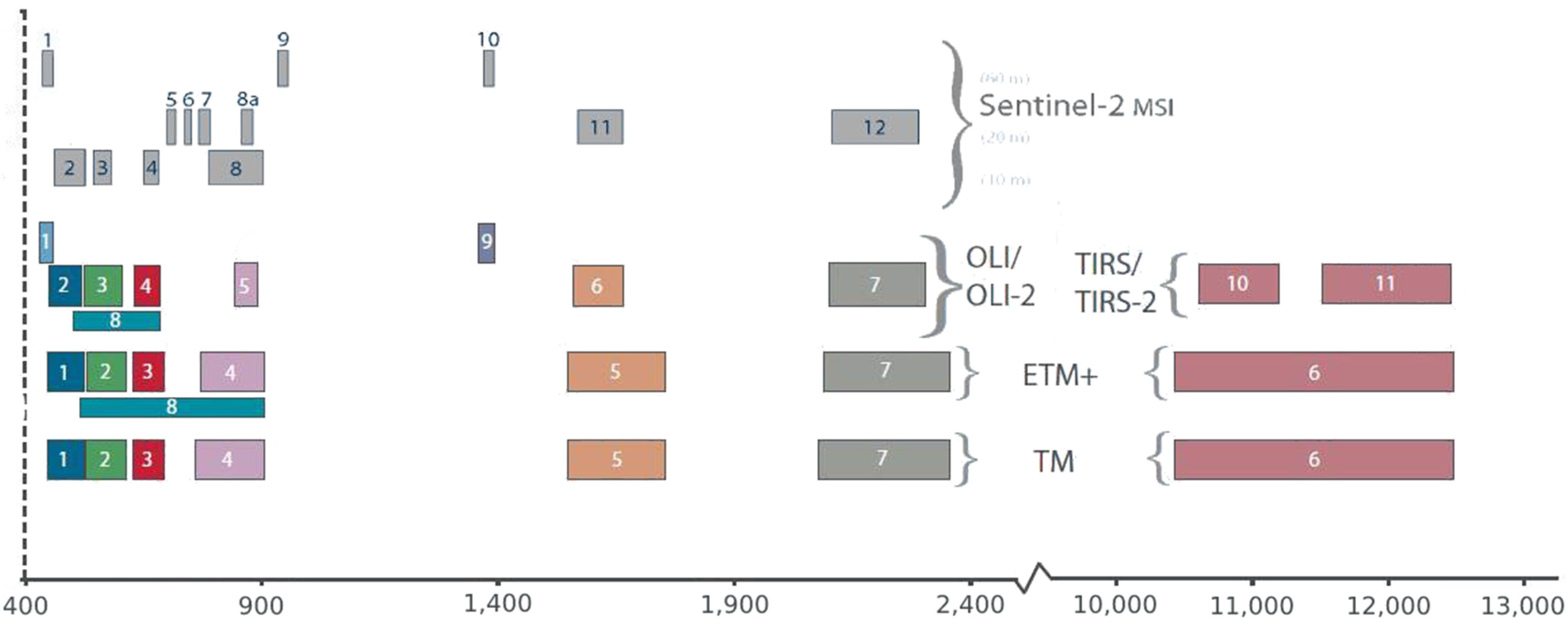
2.1. Satellite Images: Landsat and Sentinel
2.2. Vegetation Indices (VIs)
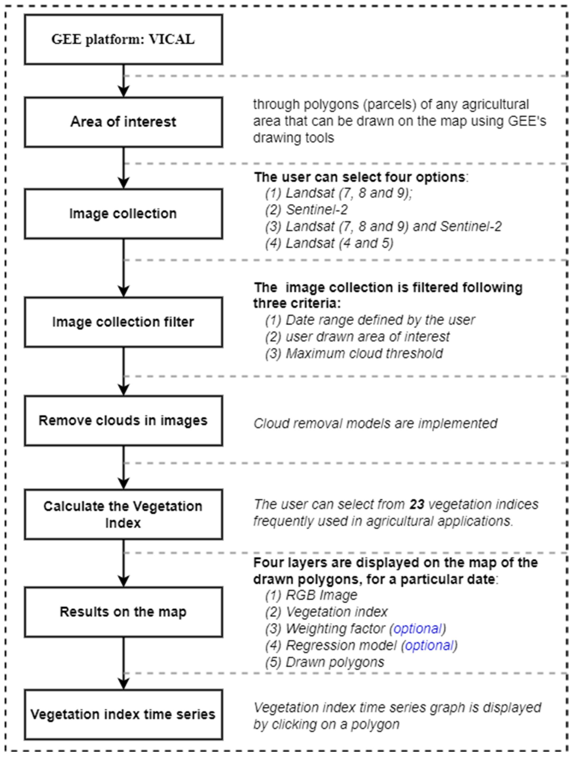
2.3. Tool Development in the Google Earth Engine (GEE) Platform
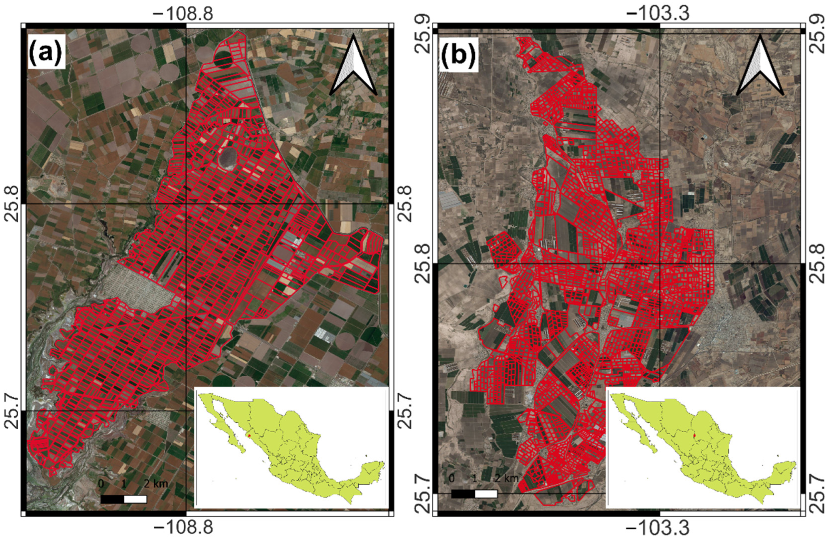
2.4. VICAL Performance Analyses
3. Results
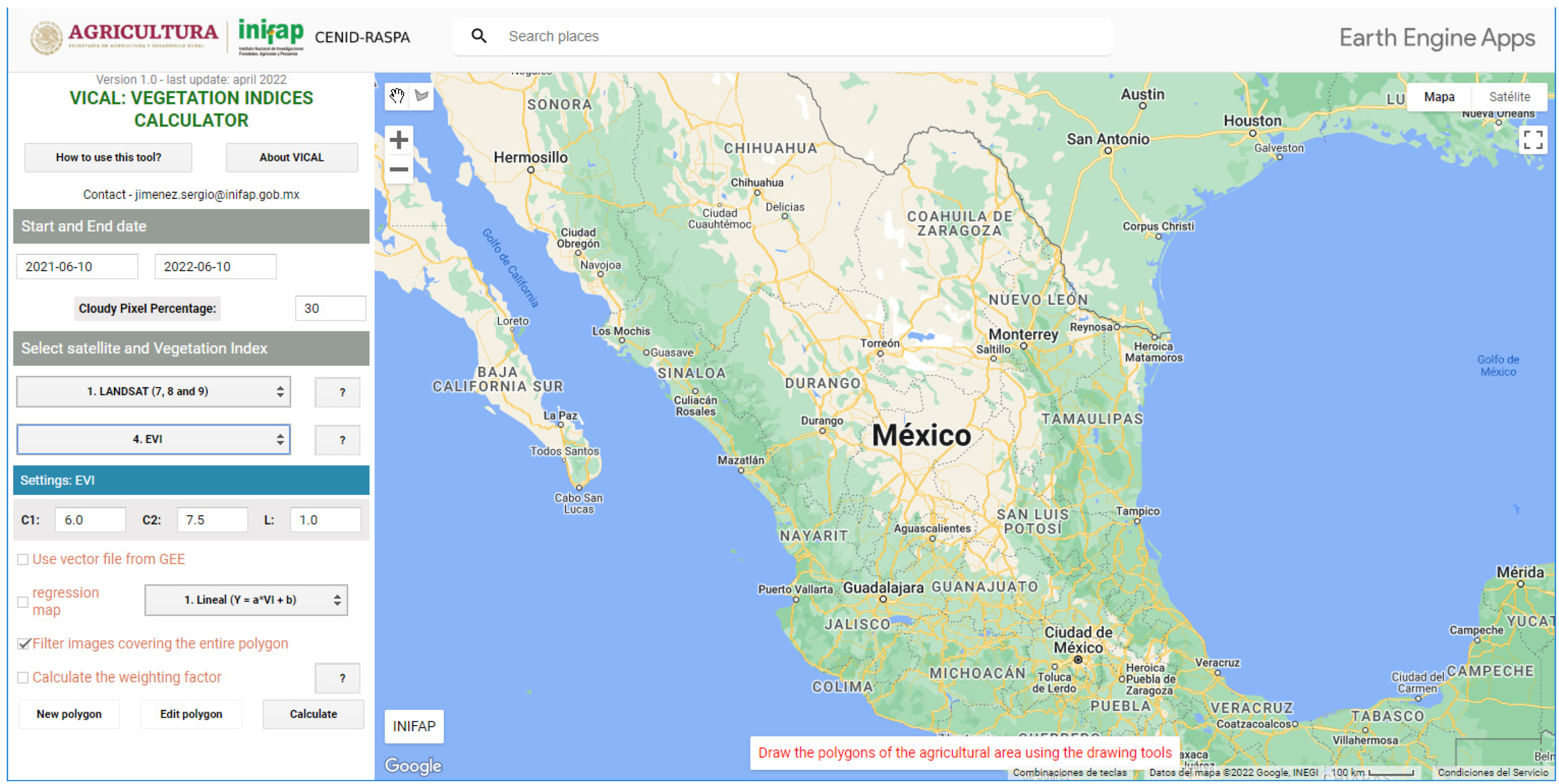
3.1. Tool Development
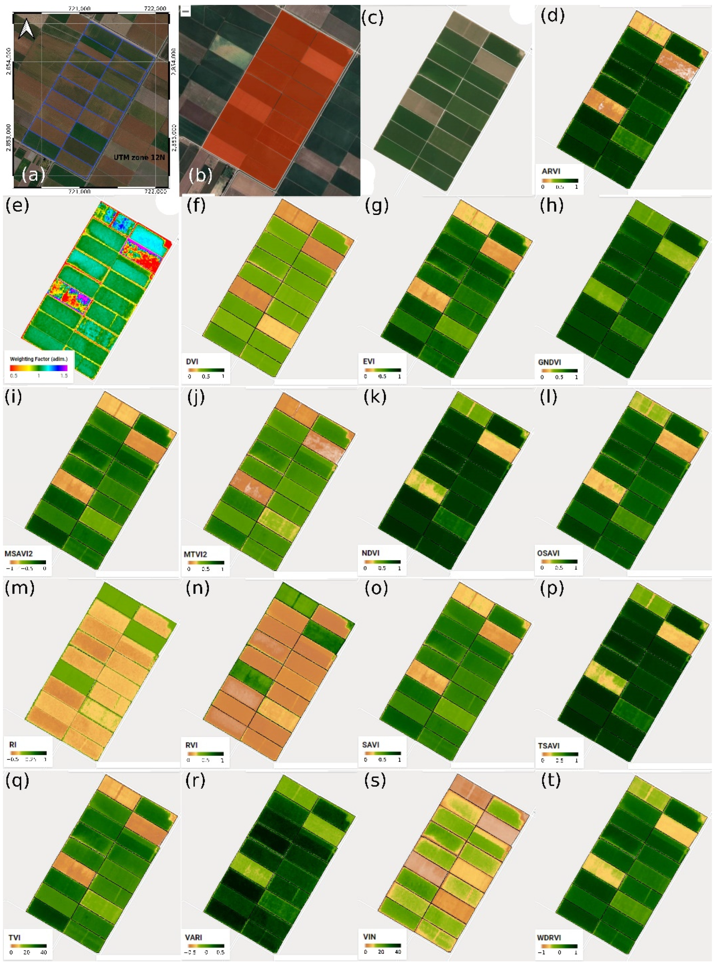
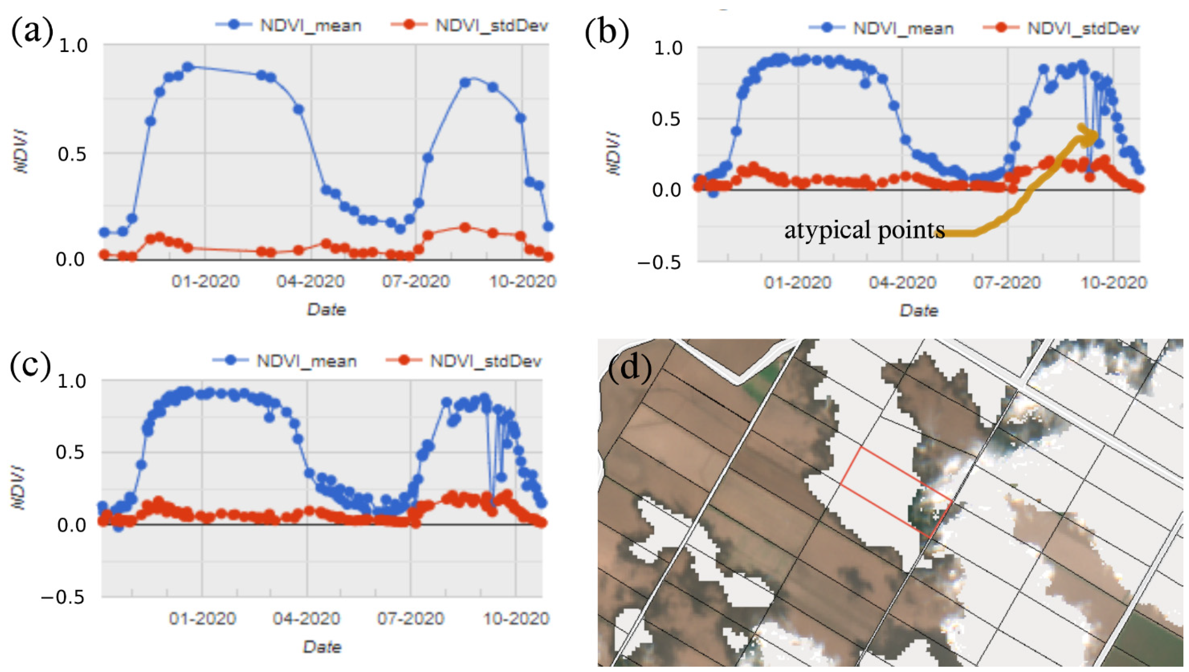
3.2. Vegetation Index (VI) Map and Time Series
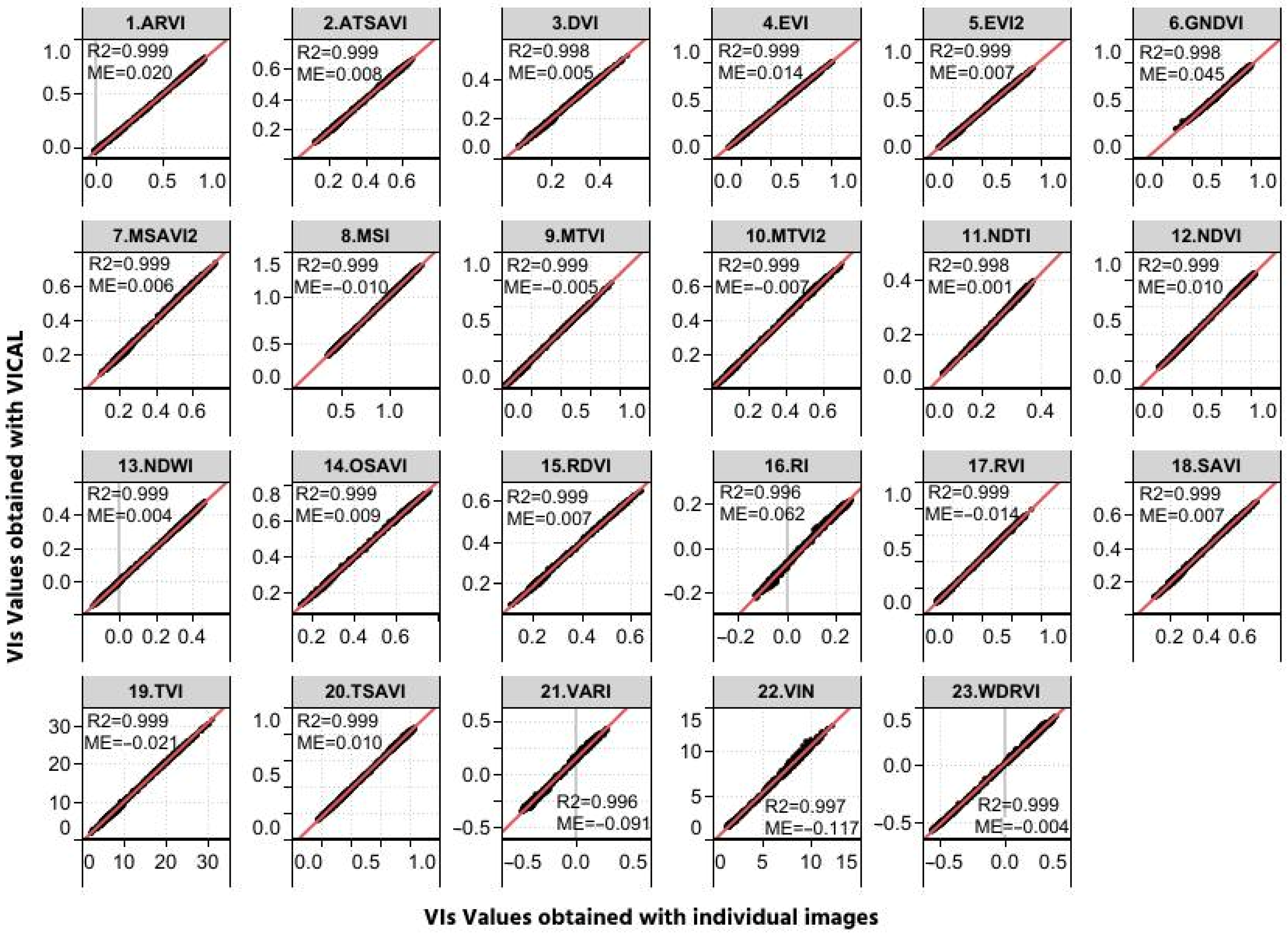
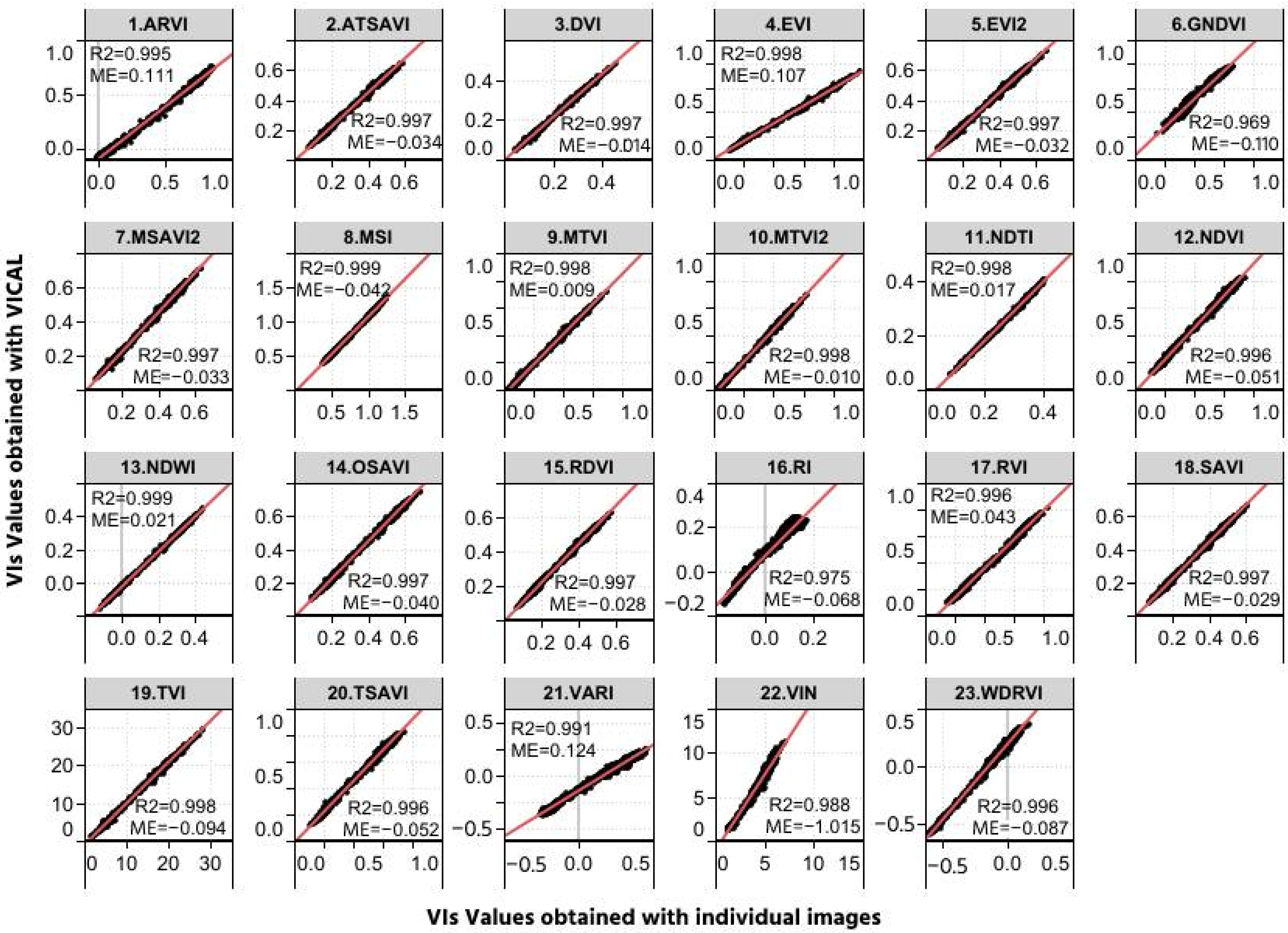
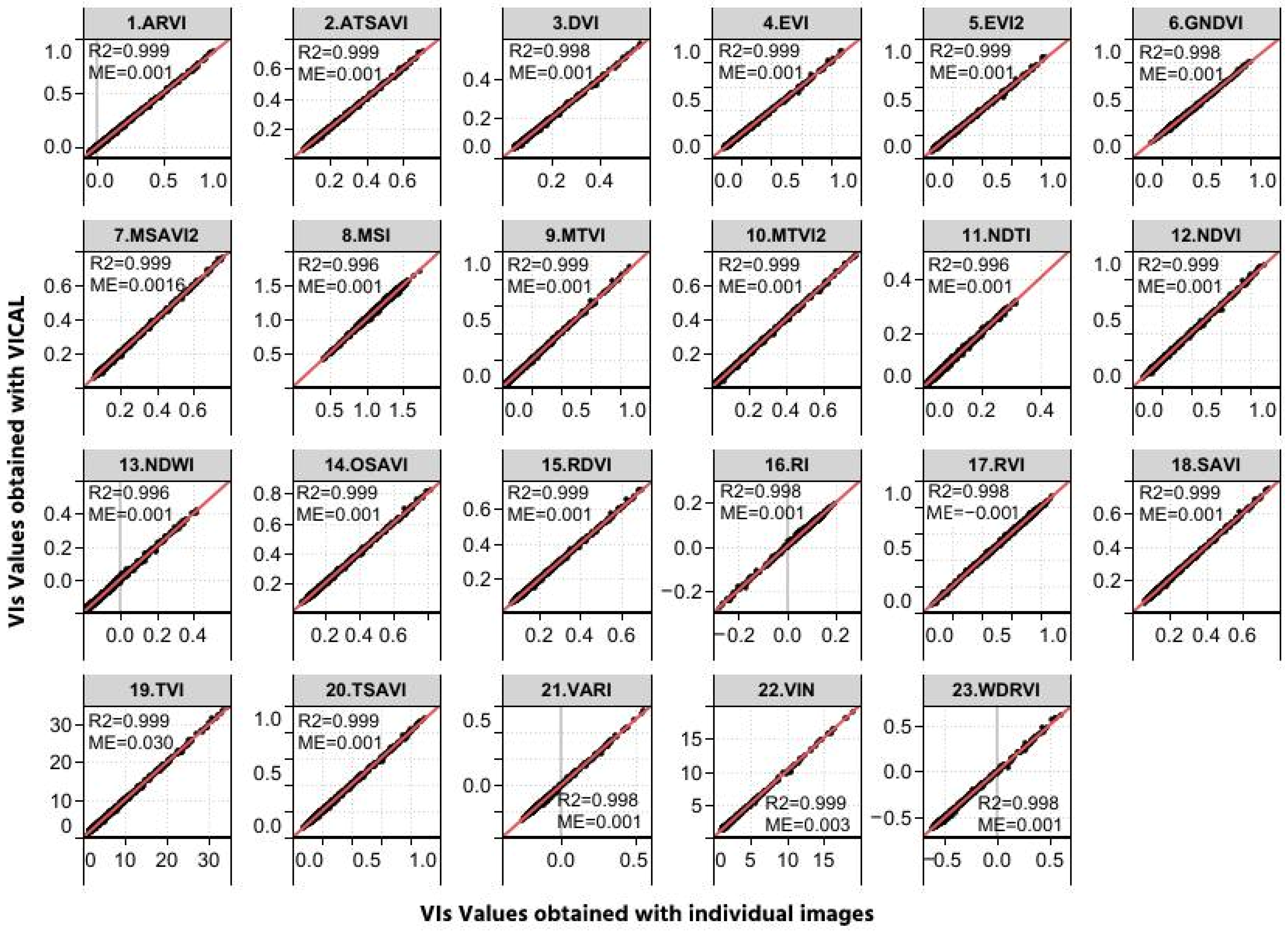
3.3. Performance Analyses
3.4. Future Perspectives
4. Conclusions
Supplementary Materials
Author Contributions
Funding
Institutional Review Board Statement
Informed Consent Statement
Data Availability Statement
Conflicts of Interest
References
- Bannari, A.; Morin, D.; Bonn, F.; Huete, A.R. A Review of Vegetation Indices. Remote Sens. Rev. 2009, 13, 95–120. [Google Scholar] [CrossRef]
- Haboudane, D.; Miller, J.R.; Pattey, E.; Zarco-Tejada, P.J.; Strachan, I.B. Hyperspectral Vegetation Indices and Novel Algorithms for Predicting Green LAI of Crop Canopies: Modeling and Validation in the Context of Precision Agriculture. Remote Sens. Environ. 2004, 90, 337–352. [Google Scholar] [CrossRef]
- Pôças, I.; Paço, T.A.; Paredes, P.; Cunha, M.; Pereira, L.S. Estimation of Actual Crop Coefficients Using Remotely Sensed Vegetation Indices and Soil Water Balance Modelled Data. Remote Sens. 2015, 7, 2373–2400. [Google Scholar] [CrossRef] [Green Version]
- Rozenstein, O.; Haymann, N.; Kaplan, G.; Tanny, J. Estimating Cotton Water Consumption Using a Time Series of Sentinel-2 Imagery. Agric. Water Manag. 2018, 207, 44–52. [Google Scholar] [CrossRef]
- Sifuentes-Ibarra, E.; Ojeda-Bustamante, W.; Ontiveros-Capurata, R.E.; Sánchez-Cohen, I. Improving the Monitoring of Corn Phenology in Large Agricultural Areas Using Remote Sensing Data Series. Span. J. Agric. Res. 2020, 18, 23. [Google Scholar] [CrossRef]
- Baret, F.; Guyot, G. Potentials and Limits of Vegetation Indices for LAI and APAR Assessment. Remote Sens. Environ. 1991, 35, 161–173. [Google Scholar] [CrossRef]
- Ren, H.; Zhou, G. Estimating Green Biomass Ratio with Remote Sensing in Arid Grasslands. Ecol. Indic. 2019, 98, 568–574. [Google Scholar] [CrossRef]
- Ren, H.; Zhou, G.; Zhang, F. Using Negative Soil Adjustment Factor in Soil-Adjusted Vegetation Index (SAVI) for Aboveground Living Biomass Estimation in Arid Grasslands. Remote Sens. Environ. 2018, 209, 439–445. [Google Scholar] [CrossRef]
- Xue, J.; Su, B. Significant Remote Sensing Vegetation Indices: A Review of Developments and Applications. J. Sens. 2017, 2017, 1353691. [Google Scholar] [CrossRef] [Green Version]
- Chen, J.; Chen, J.; Liao, A.; Cao, X.; Chen, L.; Chen, X.; He, C.; Han, G.; Peng, S.; Lu, M.; et al. Global Land Cover Mapping at 30 m Resolution: A POK-Based Operational Approach. ISPRS J. Photogramm. Remote Sens. 2015, 103, 7–27. [Google Scholar] [CrossRef] [Green Version]
- Rasmussen, J.; Azim, S.; Boldsen, S.K.; Nitschke, T.; Jensen, S.M.; Nielsen, J.; Christensen, S. The Challenge of Reproducing Remote Sensing Data from Satellites and Unmanned Aerial Vehicles (UAVs) in the Context of Management Zones and Precision Agriculture. Precis. Agric. 2021, 22, 834–851. [Google Scholar] [CrossRef]
- Zhu, Z. Change Detection Using Landsat Time Series: A Review of Frequencies, Preprocessing, Algorithms, and Applications. ISPRS J. Photogramm. Remote Sens. 2017, 130, 370–384. [Google Scholar] [CrossRef]
- Amani, M.; Ghorbanian, A.; Ahmadi, S.A.; Kakooei, M.; Moghimi, A.; Mirmazloumi, S.M.; Moghaddam, S.H.A.; Mahdavi, S.; Ghahremanloo, M.; Parsian, S.; et al. Google Earth Engine Cloud Computing Platform for Remote Sensing Big Data Applications: A Comprehensive Review. IEEE J. Sel. Top. Appl. Earth Obs. Remote Sens. 2020, 13, 5326–5350. [Google Scholar] [CrossRef]
- Gorelick, N.; Hancher, M.; Dixon, M.; Ilyushchenko, S.; Thau, D.; Moore, R. Google Earth Engine: Planetary-Scale Geospatial Analysis for Everyone. Remote Sens. Environ. 2017, 202, 18–27. [Google Scholar] [CrossRef]
- Chaves, M.E.D.; Picoli, M.C.A.; Sanches, I.D. Recent Applications of Landsat 8/OLI and Sentinel-2/MSI for Land Use and Land Cover Mapping: A Systematic Review. Remote Sens. 2020, 12, 3062. [Google Scholar] [CrossRef]
- USGS. Landsat 7|U.S. Geological Survey. Available online: https://www.usgs.gov/landsat-missions/landsat-7 (accessed on 10 January 2022).
- Claverie, M.; Ju, J.; Masek, J.G.; Dungan, J.L.; Vermote, E.F.; Roger, J.C.; Skakun, S.V.; Justice, C. The Harmonized Landsat and Sentinel-2 Surface Reflectance Data Set. Remote Sens. Environ. 2018, 219, 145–161. [Google Scholar] [CrossRef]
- Segarra, J.; Buchaillot, M.L.; Araus, J.L.; Kefauver, S.C. Remote Sensing for Precision Agriculture: Sentinel-2 Improved Features and Applications. Agronomy 2020, 10, 641. [Google Scholar] [CrossRef]
- Li, J.; Roy, D.P. A Global Analysis of Sentinel-2A, Sentinel-2B and Landsat-8 Data Revisit Intervals and Implications for Terrestrial Monitoring. Remote Sens. 2017, 9, 902. [Google Scholar] [CrossRef] [Green Version]
- NASA. Sentinel-2A Launches—Our Compliments & Our Complements-Landsat Science. Available online: https://landsat.gsfc.nasa.gov/article/sentinel-2a-launches-our-compliments-our-complements/ (accessed on 5 December 2021).
- Kaufman, Y.J.; Tanré, D. Atmospherically Resistant Vegetation Index (ARVI) for EOS-MODIS. IEEE Trans. Geosci. Remote Sens. 1992, 30, 261–270. [Google Scholar] [CrossRef]
- Colombo, R.; Bellingeri, D.; Fasolini, D.; Marino, C.M. Retrieval of Leaf Area Index in Different Vegetation Types Using High Resolution Satellite Data. Remote Sens. Environ. 2003, 86, 120–131. [Google Scholar] [CrossRef]
- Mudereri, B.T.; Dube, T.; Adel-Rahman, E.M.; Niassy, S.; Kimathi, E.; Khan, Z.; Landmann, T. A Comparative Analysis of Planetscope and Sentinel Sentinel-2 Space-Borne Sensors in Mapping Striga Weed Using Guided Regularised Random Forest Classification Ensemble. In Proceedings of the International Archives of the Photogrammetry, Remote Sensing and Spatial Information Sciences-ISPRS Archives, Milan, Italy, 8–10 May 2019. [Google Scholar]
- Shen, L.; He, Y.; Guo, X. Suitability of the Normalized Difference Vegetation Index and the Adjusted Transformed Soil-Adjusted Vegetation Index for Spatially Characterizing Loggerhead Shrike Habitats in North American Mixed Prairie. J. Appl. Remote Sens. 2013, 7, 073574. [Google Scholar] [CrossRef]
- Broge, N.H.; Mortensen, J.V. Deriving Green Crop Area Index and Canopy Chlorophyll Density of Winter Wheat from Spectral Reflectance Data. Remote Sens. Environ. 2002, 81, 45–57. [Google Scholar] [CrossRef]
- He, Y.; Guo, X.; Wilmshurst, J.F. Reflectance Measures of Grassland Biophysical Structure. Int. J. Remote Sens. 2009, 30, 2509–2521. [Google Scholar] [CrossRef]
- Richardson, A.J.; Wiegand, C.L. Distinguishing Vegetation from Soil Background Information. Photogramm. Eng. Remote Sens. 1977, 43, 1541–1552. [Google Scholar]
- Skakun, S.; Vermote, E.; Franch, B.; Roger, J.C.; Kussul, N.; Ju, J.; Masek, J. Winter Wheat Yield Assessment from Landsat 8 and Sentinel-2 Data: Incorporating Surface Reflectance, Through Phenological Fitting, into Regression Yield Models. Remote Sens. 2019, 11, 1768. [Google Scholar] [CrossRef] [Green Version]
- Yan, K.; Gao, S.; Chi, H.; Qi, J.; Song, W.; Tong, Y.; Mu, X.; Yan, G. Evaluation of the Vegetation-Index-Based Dimidiate Pixel Model for Fractional Vegetation Cover Estimation. IEEE Trans. Geosci. Remote Sens. 2021, 60, 1–14. [Google Scholar] [CrossRef]
- Huete, A.; Didan, K.; Miura, T.; Rodriguez, E.P.; Gao, X.; Ferreira, L.G. Overview of the Radiometric and Biophysical Performance of the MODIS Vegetation Indices. Remote Sens. Environ. 2002, 83, 195–213. [Google Scholar] [CrossRef]
- Wang, J.; Xiao, X.; Bajgain, R.; Starks, P.; Steiner, J.; Doughty, R.B.; Chang, Q. Estimating Leaf Area Index and Aboveground Biomass of Grazing Pastures Using Sentinel-1, Sentinel-2 and Landsat Images. ISPRS J. Photogramm. Remote Sens. 2019, 154, 189–201. [Google Scholar] [CrossRef] [Green Version]
- Fang, H.; Liang, S. Leaf Area Index Models. Ref. Modul. Earth Syst. Environ. Sci. 2014, 2008, 2139–2148. [Google Scholar] [CrossRef]
- Jiang, Z.; Huete, A.R.; Didan, K.; Miura, T. Development of a Two-Band Enhanced Vegetation Index without a Blue Band. Remote Sens. Environ. 2008, 112, 3833–3845. [Google Scholar] [CrossRef]
- Zhang, X.; Wang, J.; Henebry, G.M.; Gao, F. Development and Evaluation of a New Algorithm for Detecting 30 m Land Surface Phenology from VIIRS and HLS Time Series. ISPRS J. Photogramm. Remote Sens. 2020, 161, 37–51. [Google Scholar] [CrossRef]
- Marcial-Pablo, M.d.J.; Ontiveros-Capurata, R.E.; Jiménez-Jiménez, S.I.; Ojeda-Bustamante, W. Maize Crop Coefficient Estimation Based on Spectral Vegetation Indices and Vegetation Cover Fraction Derived from Uav-Based Multispectral Images. Agronomy 2021, 11, 668. [Google Scholar] [CrossRef]
- Gitelson, A.A.; Kaufman, Y.J.; Merzlyak, M.N. Use of a Green Channel in Remote Sensing of Global Vegetation from EOS-MODIS. Remote Sens. Environ. 1996, 58, 289–298. [Google Scholar] [CrossRef]
- Shanahan, J.F.; Schepers, J.S.; Francis, D.D.; Varvel, G.E.; Wilhelm, W.W.; Tringe, J.M.; Schlemmer, M.R.; Major, D.J. Use of Remote-Sensing Imagery to Estimate Corn Grain Yield. Agron. J. 2001, 93, 583–589. [Google Scholar] [CrossRef] [Green Version]
- Marcial-Pablo, M.d.J.; Gonzalez-Sanchez, A.; Jimenez-Jimenez, S.I.; Ontiveros-Capurata, R.E.; Ojeda-Bustamante, W. Estimation of Vegetation Fraction Using RGB and Multispectral Images from UAV. Int. J. Remote Sens. 2019, 40, 420–438. [Google Scholar] [CrossRef]
- Elwadie, M.E.; Pierce, F.J.; Qi, J. Remote Sensing of Canopy Dynamics and Biophysical Variables Estimation of Corn in Michigan. Agron. J. 2005, 97, 99–105. [Google Scholar] [CrossRef]
- Qi, J.; Chehbouni, A.; Huete, A.R.; Kerr, Y.H.; Sorooshian, S. A Modified Soil Adjusted Vegetation Index. Remote Sens. Environ. 1994, 48, 119–126. [Google Scholar] [CrossRef]
- Söderström, M.; Piikki, K.; Stenberg, M.; Stadig, H.; Martinsson, J. Producing Nitrogen (N) Uptake Maps in Winter Wheat by Combining Proximal Crop Measurements with Sentinel-2 and DMC Satellite Images in a Decision Support System for Farmers. Acta Agric. Scand. Sect. B Soil Plant Sci. 2017, 67, 637–650. [Google Scholar] [CrossRef]
- Gholami Baghi, N.; Oldeland, J. Do Soil-Adjusted or Standard Vegetation Indices Better Predict above Ground Biomass of Semi-Arid, Saline Rangelands in North-East Iran? Int. J. Remote Sens. 2019, 40, 8223–8235. [Google Scholar] [CrossRef]
- Hunt, E.R.; Rock, B.N. Detection of Changes in Leaf Water Content Using Near- and Middle-Infrared Reflectances. Remote Sens. Environ. 1989, 30, 43–54. [Google Scholar] [CrossRef]
- Elhag, M.; Bahrawi, J.A. Soil Salinity Mapping and Hydrological Drought Indices Assessment in Arid Environments Based on Remote Sensing Techniques. Geosci. Instrum. Methods Data Syst. 2017, 6, 149–158. [Google Scholar] [CrossRef] [Green Version]
- Welikhe, P.; Quansah, J.E.; Fall, S.; McElhenney, W. Estimation of Soil Moisture Percentage Using LANDSAT-Based Moisture Stress Index. J. Remote Sens. GIS 2017, 6. [Google Scholar] [CrossRef]
- Xing, N.; Huang, W.; Xie, Q.; Shi, Y.; Ye, H.; Dong, Y.; Wu, M.; Sun, G.; Jiao, Q. A Transformed Triangular Vegetation Index for Estimating Winter Wheat Leaf Area Index. Remote Sens. 2020, 12, 16. [Google Scholar] [CrossRef] [Green Version]
- Zarco-Tejada, P.J.; Ustin, S.L.; Whiting, M.L. Temporal and Spatial Relationships between Within-Field Yield Variability in Cotton and High-Spatial Hyperspectral Remote Sensing Imagery. Agron. J. 2005, 97, 641–653. [Google Scholar] [CrossRef] [Green Version]
- Abd-El Monsef, H.; Smith, S.E.; Rowland, D.L.; Abd El Rasol, N. Using Multispectral Imagery to Extract a Pure Spectral Canopy Signature for Predicting Peanut Maturity. Comput. Electron. Agric. 2019, 162, 561–572. [Google Scholar] [CrossRef]
- Liu, J.; Pattey, E.; Jégo, G. Assessment of Vegetation Indices for Regional Crop Green LAI Estimation from Landsat Images over Multiple Growing Seasons. Remote Sens. Environ. 2012, 123, 347–358. [Google Scholar] [CrossRef]
- Sun, Q.; Jiao, Q.; Qian, X.; Liu, L.; Liu, X.; Dai, H. Improving the Retrieval of Crop Canopy Chlorophyll Content Using Vegetation Index Combinations. Remote Sens. 2021, 13, 470. [Google Scholar] [CrossRef]
- Cui, B.; Zhao, Q.; Huang, W.; Song, X.; Ye, H.; Zhou, X. A New Integrated Vegetation Index for the Estimation of Winter Wheat Leaf Chlorophyll Content. Remote Sens. 2019, 11, 974. [Google Scholar] [CrossRef] [Green Version]
- Van Deventer, A.P.; Ward, A.D.; Gowda, P.M.; Lyon, J.G. Using Thematic Mapper Data to Identify Contrasting Soil Plains and Tillage Practices. Photogramm. Eng. Remote Sens. 1997, 63, 87–93. [Google Scholar]
- Sonmez, N.K.; Slater, B. Measuring Intensity of Tillage and Plant Residue Cover Using Remote Sensing. Eur. J. Remote Sens. 2016, 49, 121–135. [Google Scholar] [CrossRef] [Green Version]
- Beeson, P.C.; Daughtry, C.S.T.; Wallander, S.A. Estimates of Conservation Tillage Practices Using Landsat Archive. Remote Sens. 2020, 12, 2665. [Google Scholar] [CrossRef]
- Eskandari, I.; Navid, H.; Rangzan, K. Evaluating Spectral Indices for Determining Conservationand Conventional Tillage Systems in a Vetch-Wheat Rotation. Int. Soil Water Conserv. Res. 2016, 4, 93–98. [Google Scholar] [CrossRef] [Green Version]
- Rouse, J.W.; Haas, R.H.; Schell, J.A.; Deering, D.W. Monitoring Vegetation Systems in the Great Plains with ERTS. In Proceedings of the Third ERTS Symposium, Washington, DC, USA, 10–14 December 1973; Freden, S., Mercanti, E., Becker, M., Eds.; NASA: Washington, DC, USA, 1973; pp. 309–317. [Google Scholar]
- Singh, R.K.; Irmak, A. Estimation of Crop Coefficients Using Satellite Remote Sensing. J. Irrig. Drain. Eng. 2009, 135, 597–608. [Google Scholar] [CrossRef]
- Duchemin, B.; Hadria, R.; Erraki, S.; Boulet, G.; Maisongrande, P.; Chehbouni, A.; Escadafal, R.; Ezzahar, J.; Hoedjes, J.; Kharrou, M.H.; et al. Monitoring Wheat Phenology and Irrigation in Central Morocco: On the Use of Relationships between Evapotranspiration, Crops Coefficients, Leaf Area Index and Remotely-Sensed Vegetation Indices. Agric. Water Manag. 2006, 79, 1–27. [Google Scholar] [CrossRef]
- Gao, B.C. NDWI A Normalized Difference Water Index for Remote Sensing of Vegetation Liquid Water From Space. Remote Sens. Environ. 1996, 58, 257–266. [Google Scholar] [CrossRef]
- Jackson, T.J.; Chen, D.; Cosh, M.; Li, F.; Anderson, M.; Walthall, C.; Doriaswamy, P.; Hunt, E.R. Vegetation Water Content Mapping Using Landsat Data Derived Normalized Difference Water Index for Corn and Soybeans. Remote Sens. Environ. 2004, 92, 475–482. [Google Scholar] [CrossRef]
- Huang, J.; Chen, D.; Cosh, M.H. Sub-Pixel Reflectance Unmixing in Estimating Vegetation Water Content and Dry Biomass of Corn and Soybeans Cropland Using Normalized Difference Water Index (NDWI) from Satellites. Int. J. Remote Sens. 2009, 30, 2075–2104. [Google Scholar] [CrossRef]
- Rondeaux, G.; Steven, M.; Baret, F. Optimization of Soil-Adjusted Vegetation Indices. Remote Sens. Environ. 1996, 55, 95–107. [Google Scholar] [CrossRef]
- Ihuoma, S.O.; Madramootoo, C.A. Sensitivity of Spectral Vegetation Indices for Monitoring Water Stress Intomato Plants. Comput. Electron. Agric. 2019, 163, 104860. [Google Scholar] [CrossRef]
- Roujean, J.L.; Breon, F.M. Estimating PAR Absorbed by Vegetation from Bidirectional Reflectance Measurements. Remote Sens. Environ. 1995, 51, 375–384. [Google Scholar] [CrossRef]
- Escadafal, R.; Huete, A. Étude Des Propriétés Spectrales Des Sols Arides Appliquée à Lamélioration Des Indices de Vegetation Obtenus Par Télédection. C. R. Acad. Sci. Paris 1991, 312, 1385–1391. [Google Scholar]
- Yao, H.; Huang, Y.; Hruska, Z.; Thomson, S.J.; Reddy, K.N. Using Vegetation Index and Modified Derivative for Early Detection of Soybean Plant Injury from Glyphosate. Comput. Electron. Agric. 2012, 89, 145–157. [Google Scholar] [CrossRef]
- Zhao, J.; Zhang, Y.; Tan, Z.; Song, Q.; Liang, N.; Yu, L.; Zhao, J. Using Digital Cameras for Comparative Phenological Monitoring in an Evergreen Broad-Leaved Forest and a Seasonal Rain Forest. Ecol. Inform. 2012, 10, 65–72. [Google Scholar] [CrossRef]
- Pearson, R.L.; Miller, L.D. Remote Mapping of Standing Crop Biomass for Estimation of the Productivity of Shortgrass Prairie, Pawnee National Grasslands, Colorado. In Proceedings of the 8th International Symposium on Remote Sensing of the Environment, Ann Arbor, MI, USA, 2–6 October 1972. [Google Scholar]
- Huete, A.R. A Soil-Adjusted Vegetation Index (SAVI). Remote Sens. Environ. 1988, 25, 295–309. [Google Scholar] [CrossRef]
- Odi-Lara, M.; Campos, I.; Neale, C.M.U.; Ortega-Farías, S.; Poblete-Echeverría, C.; Balbontín, C.; Calera, A. Estimating Evapotranspiration of an Apple Orchard Using a Remote Sensing-Based Soil Water Balance. Remote Sens. 2016, 8, 253. [Google Scholar] [CrossRef] [Green Version]
- Broge, N.H.; Leblanc, E. Comparing Prediction Power and Stability of Broadband and Hyperspectral Vegetation Indices for Estimation of Green Leaf Area Index and Canopy Chlorophyll Density. Remote Sens. Environ. 2001, 76, 156–172. [Google Scholar] [CrossRef]
- Baret, F.; Guyot, G.; Major, D.J. TSAVI: A Vegetation Index Which Minimizes Soil Brightness Effects on LAI and APAR Estimation. In Proceedings of the 12th Canadian Symposium on Remote Sensing Geoscience and Remote Sensing Symposium, Vancouver, BC, Canada, 10–14 July 1989; IEEE: Piscataway, NJ, USA, 1989; Volume 3, pp. 1355–1358. [Google Scholar]
- Li, Z.; Guo, X. A Suitable Vegetation Index for Quantifying Temporal Variation of Leaf Area Index (LAI) in Semiarid Mixed Grassland. Can. J. Remote Sens. 2010, 36, 709–721. [Google Scholar] [CrossRef]
- Marino, S.; Alvino, A. Hyperspectral Vegetation Indices for Predicting Onion (Allium cepa L.) Yield Spatial Variability. Comput. Electron. Agric. 2015, 116, 109–117. [Google Scholar] [CrossRef]
- Gitelson, A.A.; Kaufman, Y.J.; Stark, R.; Rundquist, D. Novel Algorithms for Remote Estimation of Vegetation Fraction. Remote Sens. Environ. 2002, 80, 76–87. [Google Scholar] [CrossRef] [Green Version]
- Viña, A.; Gitelson, A.A.; Rundquist, D.C.; Keydan, G.; Leavitt, B.; Schepers, J. Monitoring Maize (Zea mays L.) Phenology with Remote Sensing. Agron. J. 2004, 96, 1139–1147. [Google Scholar] [CrossRef]
- Ballesteros, R.; Moreno, M.A.; Barroso, F.; González-Gómez, L.; Ortega, J.F. Assessment of Maize Growth and Development with High- and Medium-resolution Remote Sensing Products. Agronomy 2021, 11, 940. [Google Scholar] [CrossRef]
- Pipatsitee, P.; Eiumnoh, A.; Praseartkul, P.; Ponganan, N.; Taota, K.; Kongpugdee, S.; Sakulleerungroj, K.; Cha-Um, S. Non-Destructive Leaf Area Estimation Model for Overall Growth Performances in Relation to Yield Attributes of Cassava (Manihot Esculenta Cranz) under Water Deficit Conditions. Not. Bot. Horti Agrobot. Cluj-Napoca 2019, 47, 580–591. [Google Scholar] [CrossRef] [Green Version]
- Nguy-Robertson, A.; Gitelson, A.; Peng, Y.; Viña, A.; Arkebauer, T.; Rundquist, D. Green Leaf Area Index Estimation in Maize and Soybean: Combining Vegetation Indices to Achieve Maximal Sensitivity. Agron. J. 2012, 104, 1336–1347. [Google Scholar] [CrossRef] [Green Version]
- Zumo, I.M.; Hashim, M.; Hassan, N. Mapping Grass Above-Ground Biomass of Grazinglands Using Satellite Remote Sensing. Geocarto Int. 2021, 1–14. [Google Scholar] [CrossRef]
- Gitelson, A.A. Wide Dynamic Range Vegetation Index for Remote Quantification of Biophysical Characteristics of Vegetation. J. Plant Physiol. 2004, 161, 165–173. [Google Scholar] [CrossRef] [Green Version]
- Sakamoto, T.; Wardlow, B.D.; Gitelson, A.A. Detecting Spatiotemporal Changes of Corn Developmental Stages in the U.S. Corn Belt Using MODIS WDRVI Data. IEEE Trans. Geosci. Remote Sens. 2011, 49, 1926–1936. [Google Scholar] [CrossRef] [Green Version]
- Dempewolf, J.; Adusei, B.; Becker-Reshef, I.; Hansen, M.; Potapov, P.; Khan, A.; Barker, B. Wheat Yield Forecasting for Punjab Province from Vegetation Index Time Series and Historic Crop Statistics. Remote Sens. 2014, 6, 9653–9675. [Google Scholar] [CrossRef] [Green Version]
- Tamiminia, H.; Salehi, B.; Mahdianpari, M.; Quackenbush, L.; Adeli, S.; Brisco, B. Google Earth Engine for Geo-Big Data Applications: A Meta-Analysis and Systematic Review. ISPRS J. Photogramm. Remote Sens. 2020, 164, 152–170. [Google Scholar] [CrossRef]
- Roy, D.P.; Kovalskyy, V.; Zhang, H.K.; Vermote, E.F.; Yan, L.; Kumar, S.S.; Egorov, A. Characterization of Landsat-7 to Landsat-8 Reflective Wavelength and Normalized Difference Vegetation Index Continuity. Remote Sens. Environ. 2016, 185, 57–70. [Google Scholar] [CrossRef] [Green Version]
- Zhu, Z.; Wang, S.; Woodcock, C.E. Improvement and Expansion of the Fmask Algorithm: Cloud, Cloud Shadow, and Snow Detection for Landsats 4–7, 8, and Sentinel 2 Images. Remote Sens. Environ. 2015, 159, 269–277. [Google Scholar] [CrossRef]
- Foga, S.; Scaramuzza, P.L.; Guo, S.; Zhu, Z.; Dilley, R.D.; Beckmann, T.; Schmidt, G.L.; Dwyer, J.L.; Joseph Hughes, M.; Laue, B. Cloud Detection Algorithm Comparison and Validation for Operational Landsat Data Products. Remote Sens. Environ. 2017, 194, 379–390. [Google Scholar] [CrossRef] [Green Version]
- Laipelt, L.; Henrique Bloedow Kayser, R.; Santos Fleischmann, A.; Ruhoff, A.; Bastiaanssen, W.; Erickson, T.A.; Melton, F. Long-Term Monitoring of Evapotranspiration Using the SEBAL Algorithm and Google Earth Engine Cloud Computing. ISPRS J. Photogramm. Remote Sens. 2021, 178, 81–96. [Google Scholar] [CrossRef]
- Zupanc, A. Improving Cloud Detection with Machine Learning|by Anze Zupanc|Sentinel Hub Blog|Medium. Available online: https://medium.com/sentinel-hub/improving-cloud-detection-with-machine-learning-c09dc5d7cf13 (accessed on 12 December 2021).
- Poudel, U.; Stephen, H.; Ahmad, S. Evaluating Irrigation Performance and Water Productivity Using EEFlux ET and NDVI. Sustainability 2021, 13, 7967. [Google Scholar] [CrossRef]
- Pôças, I.; Calera, A.; Campos, I.; Cunha, M. Remote Sensing for Estimating and Mapping Single and Basal Crop Coefficientes: A Review on Spectral Vegetation Indices Approaches. Agric. Water Manag. 2020, 233, 106081. [Google Scholar] [CrossRef]
- Campos, I.; Neale, C.M.U.; Suyker, A.E.; Arkebauer, T.J.; Gonçalves, I.Z. Reflectance-Based Crop Coefficients REDUX: For Operational Evapotranspiration Estimates in the Age of High Producing Hybrid Varieties. Agric. Water Manag. 2017, 187, 140–153. [Google Scholar] [CrossRef] [Green Version]
- Shafian, S.; Rajan, N.; Schnell, R.; Bagavathiannan, M.; Valasek, J.; Shi, Y.; Olsenholler, J. Unmanned Aerial Systems-Based Remote Sensing for Monitoring Sorghum Growth and Development. PLoS ONE 2018, 13, e0196605. [Google Scholar] [CrossRef] [Green Version]
- Chander, G.; Markham, B.L.; Helder, D.L. Summary of Current Radiometric Calibration Coefficients for Landsat MSS, TM, ETM+, and EO-1 ALI Sensors. Remote Sens. Environ. 2009, 113, 893–903. [Google Scholar] [CrossRef]
- USGS. Landsat 8 Collection 1 Land Surface Reflectance Code Product Guide. Available online: https://www.usgs.gov/media/files/landsat-8-collection-1-land-surface-reflectance-code-product-guide (accessed on 5 December 2021).
- QGIS.org QGIS Geographic Information System 2022. Available online: https://qgis.org/en/site/ (accessed on 5 December 2021).
- Mutanga, O.; Kumar, L. Google Earth Engine Applications. Remote Sens. 2019, 11, 591. [Google Scholar] [CrossRef] [Green Version]
- Eklundh, L.; Jönsson, P. TIMESAT: A Software Package for Time-Series Processing and Assessment of Vegetation Dynamics. Remote Sens. Digit. Image Process. 2015, 22, 141–158. [Google Scholar] [CrossRef]
- Duarte, L.; Teodoro, A.C.; Monteiro, A.T.; Cunha, M.; Gonçalves, H. QPhenoMetrics: An Open Source Software Application to Assess Vegetation Phenology Metrics. Comput. Electron. Agric. 2018, 148, 82–94. [Google Scholar] [CrossRef]
- Araya, S.; Ostendorf, B.; Lyle, G.; Lewis, M. CropPhenology: An R Package for Extracting Crop Phenology from Time Series Remotely Sensed Vegetation Index Imagery. Ecol. Inform. 2018, 46, 45–56. [Google Scholar] [CrossRef]
- Hagolle, O.; Huc, M.; Pascual, D.V.; Dedieu, G. A Multi-Temporal Method for Cloud Detection, Applied to FORMOSAT-2, VENµS, LANDSAT and SENTINEL-2 Images. Remote Sens. Environ. 2010, 114, 1747–1755. [Google Scholar] [CrossRef] [Green Version]
- Graesser, J.; Stanimirova, R.; Friedl, M. Reconstruction of Satellite Time Series With a Dynamic Smoother. IEEE J. Sel. Top. Appl. Earth Obs. Remote Sens. 2022, 15, 1803–1813. [Google Scholar] [CrossRef]
- Kong, D.; Zhang, Y.; Gu, X.; Wang, D. A Robust Method for Reconstructing Global MODIS EVI Time Series on the Google Earth Engine. ISPRS J. Photogramm. Remote Sens. 2019, 155, 13–24. [Google Scholar] [CrossRef]


| Characteristic | Landsat 4–5/TM | Landsat 7/ETM+ | Landsat 8/OLI | Landsat 9/OLI-2 | Sentinel-2A/MSI | Sentinel-2B/MSI | |
|---|---|---|---|---|---|---|---|
| Launch date | 16 July 1982 (Landsat-4)/1 March 1984 (Landsat-5) | 15 April 1999 | 11 February 2013 | 27 September 2021 | 23 June 2015 | 7 March 2017 | |
| Repeat coverage | 16 days | 16 days | 16 days | 16 days | 10 days | ||
| Spatial resolution | 30 m/90 m (TIRS) | 30 m/60 m (TIRS) | 30 m (OLI)/100 m (TIRS) | 30 m (OLI)/100 m (TIRS) | 10 m/20 m/60 m | ||
| Swath/field of view | 183 km/15° | 180 km/15° | 180 km/15° | 290 km/20.6° | |||
| Spectral bands (central wavelength) | Ultra blue | 443 nm | 443 nm | 443 nm (60 m) | |||
| Blue (B) | 485 nm | 485 nm | 482 nm | 482 nm | 490 nm (10 m) | ||
| Green (G) | 560 nm | 560 nm | 561 nm | 561 nm | 560 nm (10 m) | ||
| Red (R) | 660 nm | 660 nm | 655 nm | 655 nm | 665 nm (10 m) | ||
| Red edge | - | - | - | 705 nm (20 m), 740 nm (20 m), 783 nm (20 m), 865 nm (20 m) | |||
| NIR | 830 nm | 835 nm | 865 nm | 865 nm | 842 nm (10 m) | ||
| SWIR1 | 1650 nm | 1650 nm | 1609 nm | 1609 nm | 1610 nm (20 m) | ||
| SWIR2 | 2215 nm | 2215 nm | 2201 nm | 2201 nm | 2190 nm (20 m) | ||
| Cirrus | - | 1373 nm | 1373 nm | 1375 nm (60 m) | |||
| Water vapor | - | - | - | 945 nm (60 m) | |||
| Thermal | 11.45 μm | 11.5 μm | 10.9 μm, 12 μm | 10.9 μm, 12 μm | – | ||
| # | Index | Abbreviation | Formula | Reference | Agricultural Application |
|---|---|---|---|---|---|
| 1 | Atmospherically resistant vegetation index | ARVI * | γ = 1.0 | [21] | LAI, weed mapping [22,23] |
| 2 | Adjusted transformed soil-adjusted vegetation index | ATSAVI * | a = 1; b = 0; X = 0.08 | [6] | Biomass, canopy height, chlorophyll content, LAI [24,25,26] |
| 3 | Difference vegetation index | DVI | NIR-R | [27] | Forecasting (predicting) crop yield, vegetation coverage [28,29] |
| 4 | Enhanced vegetation index | EVI * | C1 = 6.0, C2 = 7.5; L = 1.0 | [30] | Water consumption, biomass, LAI, phenology monitoring [5,31,32] |
| 5 | Enhanced vegetation index | EVI2 * | C1 = 2.4 | [33] | Crop coefficient, land surface phenology [34,35] |
| 6 | Green normalized difference vegetation index | GNDVI | [36] | Chlorophyll content, LAI, vegetation coverage, yield forecasting [37,38,39] | |
| 7 | Modified soil adjusted vegetation index | MSAVI2 | [40] | Biomass, nitrogen prediction, LAI [41,42] | |
| 8 | Moisture stress index | MSI | [43] | Soil moisture, soil salinity [44,45] | |
| 9 | Modified triangular vegetation index | MTVI | [2] | Monitoring phenology, LAI, vegetation water content [46,47,48] | |
| 10 | Modified triangular vegetation index-2 | MTVI2 | [2] | Chlorophyll content, LAI [49,50,51] | |
| 11 | Normalized difference tillage index (NDTI) | NDTI | [52] | Crop residue, soil tillage [53,54,55] | |
| 12 | Normalized difference vegetation index | NDVI | [56] | Crop coefficient, irrigation, monitoring phenology, vegetation coverage, vegetation water content, yield forecasting [5,35,37,38,57,58] | |
| 13 | Normalized difference water index | NDWI | [59] | Biomass, vegetation water content [60,61] | |
| 14 | Optimized soil adjusted vegetation index | OSAVI * | X = 0.16 | [62] | LAI, water stress, [47,49,63] |
| 15 | Renormalized difference vegetation index | RDVI | [64] | Biomass, canopy height, LAI, water stress [26,47,63] | |
| 16 | Redness index | RI | [65] | Phenology monitoring, plant injury detection [66,67] | |
| 17 | Ratio vegetation index | RVI | [68] | Biomass, LAI, vegetation coverage [29,32] | |
| 18 | Soil adjusted vegetation index | SAVI * | L = 0.5 | [69] | crop coefficient, evapotranspiration, vegetation coverage [8,70] |
| 19 | Triangular vegetation index | TVI | [71] | Chlorophyll content, LAI [46,51] | |
| 20 | Transformed soil adjusted vegetation index | TSAVI * | a = 1; b = 0; | [72] | Soil moisture, chlorophyll content, LAI, yield forecasting [25,73,74] |
| 21 | Visible atmospherically resistant index | VARI | [75] | Biomass, phenology monitoring, LAI, vegetation coverage [76,77,78] | |
| 22 | Vegetation index number or simple ratio | VIN | [68] | Biomass, chlorophyll content, LAI [79,80] | |
| 23 | Wide dynamic range vegetation index | WDRVI * | α = 0.2 | [81] | Crop coefficient, phenology monitoring, yield forecasting [35,82,83] |
| Sensor | Dataset Availability | Collection ID |
|---|---|---|
| Landsat-4 TM | 22 August 1982–24 June 1993 | LANDSAT/LT04/C02/T1_L2 |
| Landsat-5 TM | 16 March 1993–05 May 2012 | LANDSAT/LT05/C02/T1_L2 |
| Landsat-7 ETM+ | 28 May 1999–present | LANDSAT/LE07/C02/T1_L2 |
| Landsat-8 OLI | 11 April 2013–present | LANDSAT/LC08/C02/T1_L2 |
| Landsat-9 OLI-2 | 31 October 2021–present | LANDSAT/LC09/C02/T1_L2 |
| Sentinel-2 (MSI) | 28 March 2017–present | COPERNICUS/S2_SR_HARMONIZED |
| Band Name | Slope | Intercept |
|---|---|---|
| Blue | 0.8474 | 0.0003 |
| Green | 0.8483 | 0.0088 |
| Red | 0.9047 | 0.0061 |
| NIR | 0.8462 | 0.0412 |
| SWIR1 | 0.8937 | 0.0254 |
| SWIR2 | 0.9071 | 0.0172 |
| Band Name | Slope | Intercept | Residual |
|---|---|---|---|
| Ultra Blue | 0.996 | −0.00023 | 0.0004 |
| Blue | 0.977 | −0.00411 | 0.0018 |
| Green | 1.005 | −0.00093 | 0.0011 |
| Red | 0.982 | 0.00094 | 0.0015 |
| NIR | 1.001 | −0.00029 | 0.0003 |
| SWIR1 | 1.001 | −0.00015 | 0.0001 |
| SWIR2 | 0.996 | −0.00097 | 0.0009 |
| Function Type | Formula | Equation Number |
|---|---|---|
| lineal | (2) | |
| quadratic | (3) | |
| potential | (4) | |
| exponential | (5) |
| Location | GEE ID | Image Collection | Number of Parcel (Polygons) | Image Acquisition Date |
|---|---|---|---|---|
| Northern Sinaloa, Mexico | projects/calcium-verbena-328905/assets/Bate | Landsat-7 | 1182 | 27 May 2018 |
| Landsat-8 | 19 May 2018 | |||
| Region Lagunera, Mexico | projects/calcium-verbena-328905/assets/DR017Parce | Sentinel-2 | 1741 | 18 April 2019 |
Publisher’s Note: MDPI stays neutral with regard to jurisdictional claims in published maps and institutional affiliations. |
© 2022 by the authors. Licensee MDPI, Basel, Switzerland. This article is an open access article distributed under the terms and conditions of the Creative Commons Attribution (CC BY) license (https://creativecommons.org/licenses/by/4.0/).
Share and Cite
Jiménez-Jiménez, S.I.; Marcial-Pablo, M.d.J.; Ojeda-Bustamante, W.; Sifuentes-Ibarra, E.; Inzunza-Ibarra, M.A.; Sánchez-Cohen, I. VICAL: Global Calculator to Estimate Vegetation Indices for Agricultural Areas with Landsat and Sentinel-2 Data. Agronomy 2022, 12, 1518. https://doi.org/10.3390/agronomy12071518
Jiménez-Jiménez SI, Marcial-Pablo MdJ, Ojeda-Bustamante W, Sifuentes-Ibarra E, Inzunza-Ibarra MA, Sánchez-Cohen I. VICAL: Global Calculator to Estimate Vegetation Indices for Agricultural Areas with Landsat and Sentinel-2 Data. Agronomy. 2022; 12(7):1518. https://doi.org/10.3390/agronomy12071518
Chicago/Turabian StyleJiménez-Jiménez, Sergio Iván, Mariana de Jesús Marcial-Pablo, Waldo Ojeda-Bustamante, Ernesto Sifuentes-Ibarra, Marco Antonio Inzunza-Ibarra, and Ignacio Sánchez-Cohen. 2022. "VICAL: Global Calculator to Estimate Vegetation Indices for Agricultural Areas with Landsat and Sentinel-2 Data" Agronomy 12, no. 7: 1518. https://doi.org/10.3390/agronomy12071518
APA StyleJiménez-Jiménez, S. I., Marcial-Pablo, M. d. J., Ojeda-Bustamante, W., Sifuentes-Ibarra, E., Inzunza-Ibarra, M. A., & Sánchez-Cohen, I. (2022). VICAL: Global Calculator to Estimate Vegetation Indices for Agricultural Areas with Landsat and Sentinel-2 Data. Agronomy, 12(7), 1518. https://doi.org/10.3390/agronomy12071518