Integrating Satellite and UAV Data to Predict Peanut Maturity upon Artificial Neural Networks

Abstract

The monitoring and determination of peanut maturity are fundamental to reducing losses during digging operation. However, the methods currently used are laborious and subjective. To solve this problem, we developed models to access peanut maturity using images from unmanned aerial vehicles (UAV) and satellites. We evaluated an area of approximately 8 hectares in which a regular grid of 30 points was determined with weekly evaluations starting at 90 days after sowing. Two Artificial Neural Networking (ANN) were used with Radial Basis Function (RBF) and Multilayer Perceptron (MLP) to predict the Peanut Maturity Index (PMI) with the spectral bands available from each sensor. Several vegetation indices were used as input to the ANN, with the data being split 80/20 for training and validation, respectively. The vegetation index, Normalized Difference Red Edge Index (NDRE), was the most precise coefficient of determination (R² = 0.88) and accurate mean absolute error (MAE = 0.06) for estimating PMI, regardless of the type of ANN used. The satellite with Normalized Difference Vegetation Index (NDVI) could also determine PMI with better accuracy (MAE = 0.05) than the NDRE. The performance evaluation indicates that the RBF and MLP networks are similar in predicting peanut maturity. We concluded that satellite and UAV images can predict the maturity index with good accuracy and precision.

1. Introduction

With the changes in the production system, led by food security, limited resources, environmental preservation, reduction in arable land, and growing food demand due to population increase [1], digital agriculture emerges as an option to overcome these challenges and point to new perspectives for agribusiness [2]. Several researchers across the globe and the private sector in agriculture seek to develop tools to transform data into information using data from remote sensing associated with artificial intelligence. When this transformation is possible, growers have options to make the right decision to improve resource management in the field [3,4] and it can improve crop yields.

In this context, to improve the peanut yield and reduce pods losses, the right decision about pods’ maturity is needed. When peanut digging is performed at an inadequate time (too early or too late), it can reduce quality both quantitatively and qualitatively. This is because the increase in harvest losses is directly related to the maturity point. Pods with a high maturity level detach more easily from the gynophore; in contrast, immature pods return a lower final quality. Thus, estimating the peanut maturity index is still a challenge, and it is key for a peanut crop [5].

The Hull–Scrape method [6] is the most widely used by researchers and growers. However, it is laborious and extremely subjective, requiring significant sampling due to peanut variability in the field [7]. This method considers samples taken from the field, where maturity levels are classified based on mesocarp color. Researchers have been working on alternative solutions to modernize this method in recent years, making it more efficient while reducing human error.

It is possible to create predictive peanut maturity index (PMI) algorithms using remote sensing and digital technologies. Despite some available studies using these technics, some have demonstrated only linear relationships and model fitting [8,9,10]. Ref. [11], created software to collect information from peanut samples (destructive method) to determine the optimal harvest time remotely. The innovative method aims mainly to eliminate the subjectivity of the human eyes. However, the same authors concluded that the model must reach better levels of accuracy when the sampling is increased. Despite reducing the subjectivity of the human eye, this is still a destructive method and laborious.

Undoubtedly, an efficient, accurate, innovative, and non-destructive analytical method to determine the PMI that employs artificial intelligence models, using remote sensing data through Artificial Neural Networks (ANN), provides high expectations for the sector. This expectation is due to the ability to map field variability that coupled sensors, both UAV and satellite, can generate through a single image [12]. However, several factors can influence vegetation response. It is convenient to use robust techniques with the ability to learn complex, nonlinear patterns (e.g., ANN) for vegetation parameter prediction associated with the use of remote sensing [13].

Research to predict yield, biomass, biophysical parameters, and weed detection shows the potential use of ANN models combined with data generated from remote sensing [13,14,15,16,17]. Thus, the use of remote sensing platforms combined with ANN can create models able to predict PMI more accurately and precisely. However, little is known about the effectiveness of intelligent models associated with remote sensing data, either UAV or satellite, for estimating PMI in tropical regions, as South American, where peanut crops have a short cycle. Thus, the objectives of this study are: (1) to evaluate the potential of UAV and satellite sensors to predict peanut maturity using machine learning techniques and (2) to validate the maturity prediction performance using spectral bands and vegetation indices using ANN.

2. Materials and Methods

2.1. Study Area

The experiment was conducted in a commercial field during the 2019/20 crop season in Ribeirão Preto city, São Paulo State, Brazil (Figure 1). The peanut runner-type cultivar IAC OL3 was planted in November. This cultivar has a growing cycle of approximately 120 days and is planted in more than 75% of Brazilian peanut fields. Dumont city has a climate classification of Aw, i.e., tropical with dry winter [18].

2.2. Field Evaluations

The experiment was implemented over approximately 8 ha, in which 30 central equidistant points at 50 m were distributed. Peanut maturity assessments were performed at 75, 105, 120, and 125 days after sowing (DAS), the last date being three days before uprooting. All evaluations were performed to monitor the behavior of peanut spatial–temporal variability of the crop to generate prediction models of peanut maturation using artificial intelligence (Figure 2).

Five plants were collected per sampling point for maturity analysis. All pods of the plants in the sample were removed, obtaining 150 to 250 pods for each sampling point. The plants were chosen randomly within a 10 m radius from the center plot. Then, all pods were submitted to the process of exocarp removal with the help of a high-pressure washer, following the Hull–Scrape method [6]. The pods, after removal of the exocarp, were placed and classified on the peanut maturity board (Figure 1), considering the color column that determines the maturity of peanut pods.

The number of pods in each color classes was recorded. The sum of brown and black pods was divided by the total number of pods multiplied by 100, which was used to create the Peanut Maturity Index (PMI). When the PMI value is up to 70%, this is the ideal point to start digging [8].

2.3. UAV Image Acquisition

The aerial images were taken with a Micasense RedEdge-M camera which is able to capture five images in a single shoot in different spectral bands: Blue (465–485 nm), Green (550–570 nm), Red (658–678 nm), Near-Infrared (820–860 nm), and Red Edge (712–722 nm). The camera was on board a UAV model DJI Matrice 100 (Shenzhen, China). Before each flight, the camera was used to capture images of the calibration panel, which were used to radiometric corrections. To ensure all flights were aligned, control points were drawn with whitewash in cross shapes and placed at each vertex of the area. In addition, to extract the exact plant reflectance collected for maturity analysis, lines using whitewash were made to identify the sampling points in the images. All UAV flights followed the exact dates as the field crop assessments, with flight times ranging from 10 a.m. to 12 a.m., with altitudes of 90 m and lateral and frontal overlap of 90%. For this flight height, the spatial resolution of the camera was 7.96 cm.

The flight plan was prepared in the GSPro software. To process the images, the Pix4D software, the student version, was used to generate orthomosaics and radiometric correction of the images. The free software Qgis (QGIS Development Team, Open-Source Geospatial Foundation, Chicago, IL, USA) was used to extract the pixels referring to the soil reflectance of the aerial images through unsupervised classification (k-means method), to avoid spectral mixing of the target of interest (plant) with the soil reflectance. A 1 m radius buffer (equivalent to 3.14 m²) was created from the collection points to cover the most significant number of pixels. Subsequently, the mean value of the pixel reflectance of each sample point was extracted.

2.4. Acquisition of PlanetScope Images

Data from the PlanetScope CubeSat platform sensor for the satellite images were used. PlanetScope is a constellation of satellites comprising different types of satellites with high spatial and temporal resolution. Currently, PlanetScope has over 180 nanosatellites in solar orbit, which can collect images daily anywhere on the planet with a 3–5 m resolution and have four spectral bands: Blue (455–515 nm), Green (500–590 nm), Red (590–670 nm), Near-Infrared (780–860 nm) [19].

For image correction, PlantScope has made the Surface Reflectance product available. This product ensures consistency in localized atmospheric conditions, minimizing uncertainty in the spatial–temporal spectral response. Surface Reflectance is available for all orthorectified scenes. Image corrections are determined from the top-of-atmosphere reflectance (TOA) and are calculated from the coefficients provided with the Planet Radiance product. The surface reflectance calculation is a pixel-by-pixel operation using Lookup Tables (LUTs) generated using the 6SV2.1 radiative transfer code. The LUTs map the reflectance at the TOA to the Bottom of Atmosphere (BOA) reflectance for all selected combinations [19]. Due to the low availability of satellite images for the period because of the rainy season, with cloud presence in the region, Planet images with a maximum interval of three days were used compared to drone images.

2.5. Vegetation Indices (VIs)

We calculated seven VIs using UAV image reflectance values and six VIs for the satellite data. The mean values of the VIs and spectral bands were used as inputs to create non-linear models and, consequently, verify the platforms’ potential (UAV and Satellite) to predict peanut maturity variability in the field. All these indices were chosen because they have promising applications in predicting agronomic parameters in several crops (

Table 1. Vegetation Index (VI) for the drone and satellite.

VI	Equation	References
NDVI	(NIR − Red)/(NIR + Red)	[20]
GNDVI	(NIR − Green)/(NIR + Green)	[21]
MNLI	(NIR2 − Red) (1 + L **)/(NIR2 + Red + L **)	[22]
EVI	2.5 (NIR − Red)/(L ** + NIR + C1 ** Red − C2 **Blue)	[23]
NLI	(NIR − Red)/(NIR2 + Red)	[24]
SAVI	(1 + L **) (NIR − Red)/(L + NIR + Red)	[25]
NDRE ***	(NIR − RE)/(NIR + RE)	[26]

NDVI: Normalized Difference Vegetation Index; GNDVI: Green Normalized Difference Vegetation Index; MNLI: Modified Non-Linear Index; EVI: Enhanced Vegetation Index; NLI: Non-Linear Index; SAVI: Adjusted Vegetation Index; NDRE: Normalized Difference Red Edge Index; ** L = 0.5; C1 = 6; C2 = 7.5. *** VI not used for the satellite because the sensor does not provide the RedEdge band.

).

2.6. Statistical Analysis

The PMI response over time was analyzed using descriptive statistics using Box Plot, which was presented as a function of the accumulated degree days (aGDD) (Equation (1)). Thus, a weather station was installed to collect minimum and maximum temperature data throughout the season (Supplementary Material Figure S1).

aGDD = ((Tmax + Tmin)/2) – Tb

(1)

where Tmax is the maximum temperature, Tmin is the minimum temperature, and Tb is the lowest basal temperature for peanut production (13.3 °C).

To improve box plot analysis and obtain better visualization of peanut maturity variability on the field, the PMI maps were interpolated using the Inverse Weighted Distance (IWD) deterministic method generated in the Qgis software for each collection date.

2.7. Description of ANN Models for Prediction of PMI

Data modeling techniques were performed in which two Artificial Neural Networks (ANN) models were used to predict peanut maturity index using vegetation indices, the radial basis function (RBF), and the multilayer perceptron (MLP) type. ANNs are computational models that use artificial neurons and perform functions similar to human neurons [27]. Among the main advantages of ANN’s is that these models can learn relationships between variables and recognize patterns through examples, standardizing the learned information and developing nonlinear models [28,29]. Another factor driving the use of machine learning techniques in agriculture is the universal fit function of the models, which admits non-parametric data losses [3,27,30].

2.8. Multilayer Perceptron Neural Networks (MLP)

MLP have been successfully applied with the error back-propagation algorithm through their supervised training. This network is trained with the inputs matched to the output variable (PMI) in two stages (forward and backward). Choices such as neural network architecture, training algorithm, and associated parameters are important operations in ANN analysis. Looking to avoid a trial-and-error approach to determining these operations, the Intelligent Problem Solver (IPS) tool, that is part of the Statistica 7 (Statistica 7, StatSoft, Inc., Tulsa, OK, USA) software, was used to obtain the heuristic combination to make the topology definition easy and fast (minimal-becketing technique and simulated annealing algorithm) [31]. Using the software, it was possible to automatically test a thousand different models for prediction, network architecture, and associated parameters.

The input layers of the network were composed of the vegetation indices and spectral bands of the aerial and orbital sensors and the output layer by the PMI. The number of neurons ranged from 1 to 20 for the MLP networks and 2 to 4 hidden layers. The combinations used for the models were: satellite bands; UAV bands and satellite VIs; UAV VIs; satellite bands and VIs; UAV bands and VIs; satellite and UAV bands; satellite VIs and UAV; satellite/UAV bands/VIs; and all VIs and bands separately.

The networks are interconnected by connecting forces represented by values called synaptic weights, which are responsible for storing the acquired knowledge. The values used in the input layers were normalized according to Equation (2).

$${\mathrm{y}}_{\mathrm{i}}=\frac{{\mathrm{x}}_{\mathrm{i}}-{\mathrm{x}}_{\max }}{{\mathrm{x}}_{\max }+{\mathrm{x}}_{\min }}$$

(2)

where x_i is the value of the input vector (e.g., bands and vegetation index), x_min is the minimum value, and x_max is the maximum value observed.

The output value of each neuron in bed k is expressed by y_k= g(a_k), where g is the activation function of a_k and a_k is the synaptic function, which is a linear combination of the normalized input values and the synaptic weights, as shown in Equation (3).

$${\mathrm{a}}_{\mathrm{k}}={\displaystyle \sum }_{\mathrm{j}}{\mathrm{y}}_{\mathrm{j}}{\mathrm{w}}_{\mathrm{kj}}$$

(3)

where w_kj are the synaptic weights connecting the y_j input values with each k neuron.

The transfer or activation function in the neurons of each layer was the hyperbolic function.

$${\mathrm{g}(\mathrm{a}}_{\mathrm{k}})=\frac{{\mathrm{e}}^{\mathrm{ak}}-{ \mathrm{e}}^{-\mathrm{ak}}}{{\mathrm{e}}^{\mathrm{ak}}{+\mathrm{e}}^{-\mathrm{ak}}}$$

(4)

2.9. Radial Basis Activation Function (RBF)

The layers surrounding RBF are:

• the input layer,
• a hidden layer that applies a non-linear transformation from the input space to the hidden space, and
• the linear output layer seeks to classify patterns received from the hidden layer.

For RBF nets, it is only necessary to define the training algorithm and a smoothing factor, which were determined by the IPS tool.

RBF nets, such as MLP nets, are multilayer nets; however, the sigmoid activation function of neurons in the RBF hidden layer is changed by another class of function, whose value decreases or increases concerning distance from a central point [32]. In this study, the Gaussian function used for the RBF network (Equation (5)) was the radial basis function.

$$\phi =\exp \left(-\frac{v^2}{2{\sigma }^2}\right)$$

(5)

where v = ‖x − µ‖ is the Euclidean distance between the input vector and the center µ of the Gaussian function, and σ is the width. The Euclidean distance from the input vector to the center µ is the input to the Gaussian function, which provides the radial unit activation value.

2.10. Training, Validation, and Performance

During the training phase, the ANNs were trained 1000 times for each model for the RBF networks because the free parameters are obtained randomly. The input and output layers followed the same principle as the MLP network, and the simulations for the RBF network were also the same, as well as the number of neurons, which varied from 1 to 20.

The database was divided into 80% for training and 20% for model validation. The procedures for training and validation of neural network models were implemented in the Neural Networks package of Statistic data analysis software (Statistica 7.0, Statsoft Inc., Tulsa, OK, USA).

The efficiency of the networks was analyzed using graphics with a 1:1 ratio. Accuracy and precision were analyzed using the mean absolute error (MAE) for the prediction error and the coefficient of determination (R²) for precision, demonstrating the reliability of the data obtained from the predictions of the variables. Furthermore, comparative analyses were performed between the predicted and observed data. The accuracy and precision were evaluated by calculating MAE, and the coefficient of determination (R²) is represented by Equations (6) and (7), respectively.

$$\mathrm{MAE}=\frac{1}{n} {{\displaystyle \sum }}_{i=1}^n\left(Y_i-{\overline{Y}}_i\right)$$

(6)

$$R^2=\frac{\mathrm{SQR}}{\mathrm{SQT}}$$

(7)

where SQR is the sum of squares of the residuals and SQT is the sum of total squares.

To answer which is the best model to predict peanut maturity and which vegetation index presented the best performance in the validation step of the ANN models, the best model was the one that presented the lowest MAE value, that is, the one that presented the best accuracy (up to 0.06).

3. Results

3.1. Exploratory Analysis of PMI

The PMI variability on the field is low (<10%) when the peanut plants were 1423 aGDD at 75 days after planting (DAP). On the other hand, when the plants reached 1778 aGDD, the variability among plots increased at 105 DAP (Figure 3). The box plot shows that at 2099 aGDD, the PMI median was near to the first quartile, indicating positive asymmetric distribution, while the PMI distribution on other analyzed dates showed negative asymmetric distribution. In addition, the spatial distribution maps provide a useful visualization of peanut variability on the field, where it decreases when the peanut plants increase the aGDD and are ready to be dug.

3.2. Comparation between Remote Sensing Platforms

Among all models tested for the satellite platform, the highest accuracy (MAE = 0.05) was found using the RBF network for both inputs, bands (Bands_sat), and the combination between bands and satellite vegetation indices (B/VI_sat). The same accuracy level was found for the UAV platform using RBF networking for the model that has a combination of different VIs. In contrast, MLP models had an accuracy of 0.06, except for NDVI_sat and B/VI_sat, and the MAE was equal to 0.05 for both models (RBF and MLP) (Figure 4).

When the models were trained and validated with the variables separately, the green band from the satellite was the variable that estimated the PMI with the highest accuracy and precision using RBF. The NDVI_sat and NDRE_UAV showed the best models for the MLP network, which estimated the PMI with an accuracy of 0.05 and 0.06, respectively, and a precision of R² = 0.90 for both inputs (Figure 4).

In this research, the ANN models developed show good accuracy and precision to predict peanut maturity using remote sensing (UAV and satellite image). However, based on accuracy and precision, the UAV images presented better performance than satellite images (

Table 2. Resulting models, topologies, accuracy, and precision of ANN.

			Training		Validation
Simulation	Model	Model Structure	MAE	R2	MAE	R2
B/VI_sat *	RBF	3:20:1	0.05	0.89	0.05	0.90
	MLP	4:20–10:1	0.06	0.90	0.05	0.90
green_sat	RBF	1:14:1	0.06	0.90	0.06	0.90
	MLP	1:20–10:1	0.06	0.89	0.06	0.89
NDVI_sat	RBF	1:13–1:1	0.05	0.89	0.05	0.89
	MLP	1:1–6:1	0.05	0.90	0.05	0.90
NDRE_UAV	RBF	1:1–1:1	0.06	0.88	0.06	0.88
	MLP	1:20–10:1	0.06	0.90	0.06	0.90
Bands_sat	BRF	3:3–20:1	0.05	0.87	0.05	0.87
	MLP	4:20–8:1	0.06	0.86	0.06	0.84
Index_UAV	BRF	3:3–20:1	0.05	0.91	0.05	0.91
B/VI_UAV **	MLP	5:11–10:1	0.06	0.89	0.06	0.89

RBF: Radial Basis Function; MLP: Multilayer Perceptron; Neural network architecture is presented in the form of I:N:O, in which “I” is the number of input variables, “N” is the number of neurons in the hidden layer, and “O” is the number of output variables. * B/VI_sat = satellite bands and vegetation index; ** B/VI_UAV = UAV bands and vegetation index.

), with 15 models for each algorithm (RBF and MLP), while 13 models were found using satellite images. Despite that, the models generated using satellite platform images resulted in the best accuracies (Figure 4).

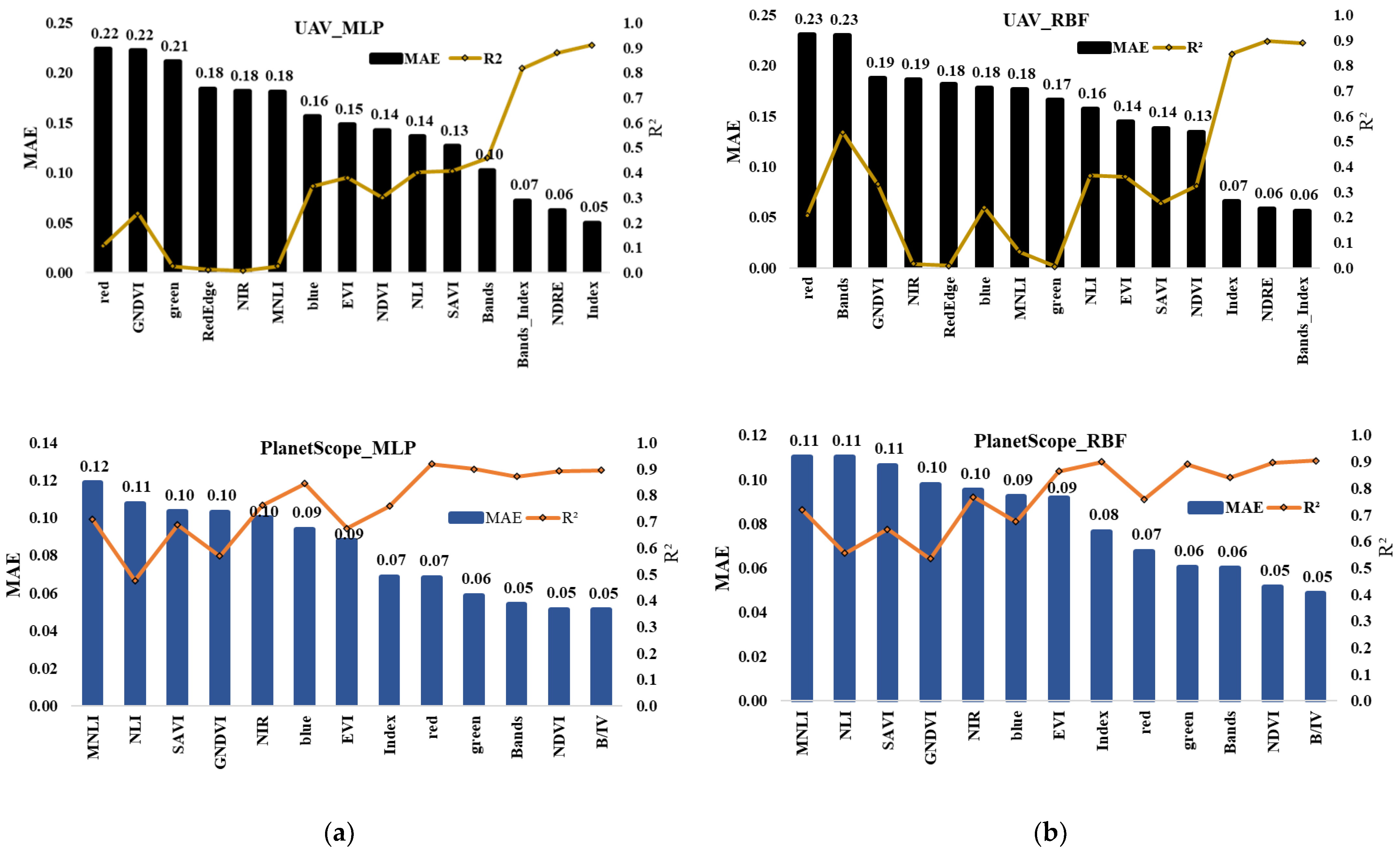
3.3. ANN Performance

Ten models for each topology combination were selected using the IPS approach, considering MAE between 0.05 and 0.06 and R² up to 0.85 in the validation step. As a result, six models for each ANN tested (RBF and MLP) showed the potential to be used when the input variables were from UAV images. In contrast, satellite images resulted in eight models (Table 2). The RBF network used three inputs for all models combined (B/IV_sat; Band_sat; Index_UAV), while the MLP network used four and five inputs (Table 2). In other words, RBF models can be more efficient than MLP due to fewer variables being required to predict the same output, and it could be more useful to growers and field assistance.

Among the topologies tested, the ANNs used 20 neurons in the first hidden layer for the simulations (B/VI_sat; Bandas_sat; Index_UAV). The MLP network used 11 neurons for B/IV_UAV in the first hidden layer and 10 in the second. For the simulations conducted for each variable separately, the RBF model used only 1 neuron in the hidden layer for NDRE_UAV, while the MLP used 20 neurons in the first hidden layer and 10 in the second. However, both models showed the same accuracy (0.06), with only a difference in precision (RBF = 0.88 and MLP = 0.90). Thus, the number of neurons in the hidden layer is not a determining factor in obtaining good ANN models to estimate maturity based on spectral data of peanut crop (Table 2).

We used sensitivity analysis to rank the importance of each input variable used in the models to predict peanut maturity (Tables S1 and S2 in the supplemental material). Based on the performance, accuracy, and precision analysis, the best ANN models using satellite platform to estimate PMI are found when the spectral bands and VI are combined (B/VI_sat) independently of the ANN type, RBF, and MLP networks. The sensitivity analysis for the RBF model used three inputs and had, as the most important variable, the NIR band, followed by the VI, EVI, and MNLI. The MLP network used the four inputs (NDVI, blue, green, and GNDVI) in importance order.

The aerial platform also showed the potential to predict peanut maturity with the vegetation indices for the RBF network. The architecture used the variables NDRE, NLI, and SAVI, with an order of importance of first, second, and third, respectively.

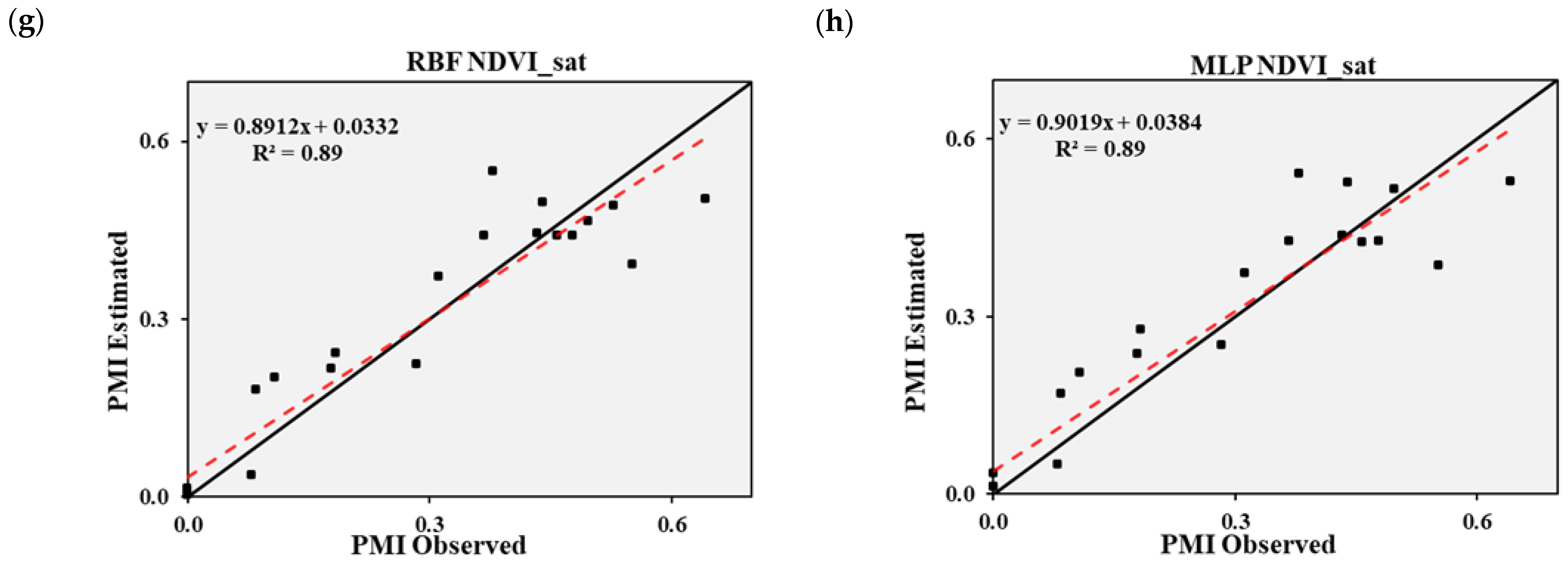
3.4. Validation Models

The performance of RBF and MLP models indicates that the networks are similar for predicting peanut maturity (Figure 5 and Figure 6). In our validation process, is important to point out that when NDV, calculated from satellite image (NDVI_sat), was used as a single input it resulted in a better fitted straight line, and the prediction values were close to the 1:1 line. The RBF model for UAV vegetation indices had the best performance in terms of accuracy and precision for the combined models.

4. Discussion

Our research developed a peanut maturity prediction model integrating orbital and airborne remote sensing. These models will improve the optimal peanut harvest point, considering peanut maturity variability. As peanut plants accumulate growing degree days, the PMI increases, showing the dependence on climate temperature to reach pod maturity [33]. Peanuts have a growth habit that is characterized as indeterminate, which causes a lot of variabilities and makes the identification of the ideal maturity point difficult. Another aspect to consider is the fact that the crop does not show visible physiological changes in leaves to indicate the senescence process in the plant. In other words, this means that, in the same plant, pods can be found in different stages of development (R2 to R8). This variability within the same plant is represented by a gynophore inside the ground containing an intumescent ovary, up to pods with 2/3 or 3/4 of the fruits fully developed, with a typical coloration varying from brown to black [34].

Despite the difficulty in identifying pod maturity, the most widespread method among growers and researchers for determining the PMI is the Hull–Scrape method [6], a destructive and subjective methodology. This method is considered subjective because the pods’ color can be seen to be different between analysts. An assertive harvest can be reaped by accurately determining the ideal point of PMI without subjectivity. Over the years, researchers showed methods to determine the best time to harvest peanuts. However, the proposed methods have significant limitations and uncertainties [11]. The use of remote sensing and machine learning technologies has been helpful for the agricultural sector, especially as an easy and non-destructive way to access the agriculture parameter [35]. However, a simple peanut prediction maturity model with good precision and accuracy is still a challenge for the peanut production sector. This model is needed because, when peanut digging is performed over mature pods, it can return quantitative and qualitative losses.

Trying to solve the main peanut issue related to maturity, [9] observed potential in the use of satellites imagens to predict peanut maturity using non-linear models. The conditions where their models were developed were similar to those of this paper, however, they only tested the Gompetz model to explain peanut maturity. Despite that, this first result was very important once they showed a decrease in the vegetation index, while the PMI increased. This response was similar to our results. Recently [10], proposed the use of RNA to predict peanut maturity in two conditions, irrigated and dryland fields using UAV and multispectral cameras, and the precision models for both fields were higher than 0.90. In this paper, we found similar model performances, especially using the RBF model as input VI calculated by UAV images (R² = 0.91—Figure 6c).

We tested combinations with multiple inputs for the models created using the bands and VIs and individual inputs to generate simpler models. The green band has already shown, in several studies, higher sensitivity to chlorophyll content (chlorophyll a and b) and biomass in monitoring the yield of corn, soybean, potato, and wheat [21,36,37,38]. For the peanut crop, refs. [8,39], using multispectral radiometer sensor and multispectral camera on UAV, respectively, found no potential in using the green band due to its low ability to determine maturity variability at different stages, contrasting with the results of this study, where the green band of the satellite was able to identify crop maturity variability accurately and precisely. The reflection of the generation of non-linear ANN models and the difference between sensors may justify the different results between the studies.

The NDVI presents limitations for vegetation with high density due to the high absorption of radiation in the red wavelength by chlorophyll pigments. However [9], using high-resolution images for the peanut crop, no evidence of saturation for NDVI was found. A result was also observed in this work in which the model generated from the satellite NDVI could express the actual variability of PMI while NDRE showed higher sensitivity to high vegetation density. In addition, our results from satellite images and RNA were more accurate than those of the model tested by [10] using NDVI as an input; we found precision levels of 89% (R² = 0.89), independently of the RNA tested (Figure 5h). Ref. [40], when evaluating the response of NDVI and NDRE for soybean cultivar, reported that NDRE did not show evidence of saturation for proximal sensors. This result was supported by hypotheses that VI which contains the red-edge band, which has been commonly reported in studies with highly dense vegetation [40,41,42].

Although the differences between sensors are apparent, such as sensor type, spatial resolution, spectral resolution, and angle of view, it is essential to look at the models generated from different platform types to generate more robust models [43]. Due to this, it is crucial to conduct research that seeks to study, in depth, the responses and information generated from different types of platforms in remote sensing, considering the distinct characteristics of the sensors and crops.

Regarding the types of networks used in this study, they belong to the same class of ANNs, called feed-forward networks, in which the information processed in the network follows a direction from the input neurons to the output neurons. There are some differences between MLP and RBF networks [44]. RBF networks are more straightforward and generally have more accessible training due to the simple, fixed three-layer structure. MLP nets work universally, and unlike RBF, all neurons define the network’s outputs. In contrast, RBF nets act as approximation nets, obtaining the outputs by specific hidden neurons [45].

5. Conclusions

The MLP and RBF neural networks had similar performances concerning the models created, which allows us to infer that these ANNs can estimate the PMI with high accuracy and precision (R² > 0.87). To monitoring the field and estimate PMI, satellite and UAV images can be used to assist growers and extension agents in preparing machines to dig peanuts. They have the option to use MLP or RBF networking; however, because of the configurations presented, the most appropriated ANN to be used is MLP, with NDVI by satellite as the input. It is important to point out that peanuts have different characteristics compared to other oil seeds, thus, evaluations under different conditions are ideal for creating more robust models. Therefore, studies are needed to verify the applicability of our models using remote sensing and ANN to predict peanut maturity in other genotypes and environments.

References

1. West, P.C.; Gerber, J.S.; Engstrom, P.M.; Mueller, N.D.; Brauman, K.A.; Carlson, K.M.; Cassidy, E.S.; Johnston, M.; MacDonald, G.K.; Ray, D.K.; et al. Leverage points for improving global food security and the environment. Science 2014, 345, 325–328. [Google Scholar] [CrossRef] [PubMed] [Green Version]
2. Radoglou-Grammatikis, P.; Sarigiannidis, P.; Lagkas, T.; Moscholios, I. A Compilation of UAV Applications for Precision Agriculture. Comput. Netw. 2020, 172, 107148. [Google Scholar] [CrossRef]
3. Jung, J.; Maeda, M.; Chang, A.; Bhandari, M.; Ashapure, A.; Landivar-Bowles, J. The Potential of Remote Sensing and Artificial Intelligence as Tools to Improve the Resilience of Agriculture Production Systems. Curr. Opin. Biotechnol. 2021, 70, 15–22. [Google Scholar] [CrossRef] [PubMed]
4. Virnodkar, S.S.; Pachghare, V.K.; Patil, V.C.; Jha, S.K. Remote Sensing and Machine Learning for Crop Water Stress Determination in Various Crops: A Critical Review. Precis. Agric. 2020, 21, 1121–1155. [Google Scholar] [CrossRef]
5. Colvin, B.C.; Tseng, Y.-C.; Tillman, B.L.; Rowland, D.L.; Erickson, J.E.; Culbreath, A.K.; Ferrell, J.A. Consideration of peg strength and disease severity in the decision to harvest peanut in southeastern USA. J. Crop Improv. 2018, 32, 287–304. [Google Scholar] [CrossRef]
6. Williams, E.J.; Drexler, J.S. A Non-Destructive Method for Determining Peanut Pod Maturity. Peanut Sci. 1981, 8, 134–141. [Google Scholar] [CrossRef]
7. Ashapure, A.; Jung, J.; Chang, A.; Oh, S.; Maeda, M.; Landivar, J. A Comparative Study of RGB and Multispectral Sensor-Based Cotton Canopy Cover Modelling Using Multi-Temporal UAS Data. Remote Sens. 2019, 11, 2757. [Google Scholar] [CrossRef] [Green Version]
8. Rowland, D.L.; Sorensen, R.B.; Butts, C.L.; Faircloth, W.H.; Sullivan, D.G. Canopy Characteristics and Their Ability to Predict Peanut Maturity. Peanut Sci. 2008, 35, 43–54. [Google Scholar] [CrossRef] [Green Version]
9. dos Santos, A.F.; Corrêa, L.N.; Lacerda, L.N.; Tedesco-Oliveira, D.; Pilon, C.; Vellidis, G.; da Silva, R.P. High-resolution satellite image to predict peanut maturity variability in commercial fields. Precis. Agric. 2021, 22, 1464–1478. [Google Scholar] [CrossRef]
10. Santos, A.F.; Lacerda, L.N.; Rossi, C.; Moreno, L.d.A.; Oliveira, M.F.; Pilon, C.; Silva, R.P.; Vellidis, G. Using UAV and Multispectral Images to Estimate Peanut Maturity Variability on Irrigated and Rainfed Fields Applying Linear Models and Artificial Neural Networks. Remote Sens. 2022, 14, 93. [Google Scholar] [CrossRef]
11. Li, R.; Zhao, Z.; Monfort, W.S.; Johnsen, K.; Tse, Z.T.H.; Leo, D.J. Development of a smartphone-based peanut data logging system. Precis. Agric. 2021, 22, 1006–1018. [Google Scholar] [CrossRef]
12. Tsouros, D.C.; Bibi, S.; Sarigiannidis, P.G. A Review on UAV-Based Applications for Precision Agriculture. Information 2019, 10, 349. [Google Scholar] [CrossRef] [Green Version]
13. de Oliveira, M.F.; dos Santos, A.F.; Kazama, E.H.; Rolim, G.D.S.; da Silva, R.P. Determination of application volume for coffee plantations using artificial neural networks and remote sensing. Comput. Electron. Agric. 2021, 184, 106096. [Google Scholar] [CrossRef]
14. Khan, I.; Iqbal, M.; Hashim, M.M. Impact of Sowing Dates on the Yield and Quality of Sugar Beet (Beta Vulgaris l.) Cv. California-Kws. Proc. Pak. Acad. Sci. Part B 2020, 57, 51–60. [Google Scholar]
15. Xie, B.; Zhang, H.K.; Xue, J. Deep Convolutional Neural Network for Mapping Smallholder Agriculture Using High Spatial Resolution Satellite Image. Sensors 2019, 19, 2398. [Google Scholar] [CrossRef] [PubMed] [Green Version]
16. Hasan, A.S.M.M.; Sohel, F.; Diepeveen, D.; Laga, H.; Jones, M.G. A survey of deep learning techniques for weed detection from images. Comput. Electron. Agric. 2021, 184, 106067. [Google Scholar] [CrossRef]
17. Ma, Y.; Zhang, Z.; Kang, Y.; Özdoğan, M. Corn Yield Prediction and Uncertainty Analysis Based on Remotely Sensed Variables Using a Bayesian Neural Network Approach. Remote Sens. Environ. 2021, 259, 112408. [Google Scholar] [CrossRef]
18. Alvares, C.A.; Stape, J.L.; Sentelhas, P.C.; Gonçalves, J.D.M.; Sparovek, G. Köppen’s Climate Classification Map for Brazil. Meteorol. Z. 2013, 22, 711–728. [Google Scholar] [CrossRef]
19. Planet. Planet Imagery Product Specification. 2020. Available online: https://assets.planet.com/marketing/PDF/Planet_Surface_Reflectance_Technical_White_Paper.pdf (accessed on 26 November 2021).
20. Rouse, J.W.; Haas, R.H.; Schell, J.A.; Deering, D.W. Monitoring Vegetation Systems in the Great Plains with Erts. NASA Spec. Publ. 1974, 351, 309. [Google Scholar]
21. Gitelson, A.A.; Merzlyak, M.N. Signature Analysis of Leaf Reflectance Spectra: Algorithm Development for Remote Sensing of Chlorophyll. J. Plant Physiol. 1996, 148, 494–500. [Google Scholar] [CrossRef]
22. Gong, P.; Pu, R.; Biging, G.S.; Larrieu, M.R. Estimation of Forest Leaf Area Index Using Vegetation Indices Derived from Hyperion Hyperspectral Data. IEEE Trans. Geosci. Remote Sens. 2003, 41, 1355–1362. [Google Scholar] [CrossRef] [Green Version]
23. Justice, C.O.; Vermote, E.; Townshend, J.R.G.; Defries, R.; Roy, D.P.; Hall, D.K.; Salomonson, V.V.; Privette, J.L.; Riggs, G.; Strahler, A.; et al. The Moderate Resolution Imaging Spectroradiometer (MODIS): Land Remote Sensing for Global Change Research. IEEE Trans. Geosci. Remote Sens. 1998, 36, 1228–1249. [Google Scholar] [CrossRef] [Green Version]
24. Goel, N.S.; Qin, W. Influences of Canopy Architecture on Relationships between Various Vegetation Indices and LAI and Fpar: A Computer Simulation. Remote Sens. Rev. 1994, 10, 309–347. [Google Scholar] [CrossRef]
25. Huete, A.R. A Soil-Adjusted Vegetation Index (SAVI). Remote Sens. Environ. 1988, 25, 295–309. [Google Scholar] [CrossRef]
26. Fitzgerald, G.; Rodriguez, D.; O’Leary, G. Measuring and Predicting Canopy Nitrogen Nutrition in Wheat Using a Spectral Index—The Canopy Chlorophyll Content Index (CCCI). Field Crops Res. 2010, 116, 318–324. [Google Scholar] [CrossRef]
27. Jiang, D.; Yang, X.; Clinton, N.; Wang, N. An Artificial Neural Network Model for Estimating Crop Yields Using Remotely Sensed Information. Int. J. Remote Sens. 2004, 25, 1723–1732. [Google Scholar] [CrossRef]
28. Savegnago, R.; Nunes, B.; Caetano, S.; Ferraudo, A.; Schmidt, G.; Ledur, M.; Munari, D. Comparison of logistic and neural network models to fit to the egg production curve of White Leghorn hens. Poult. Sci. 2011, 90, 705–711. [Google Scholar] [CrossRef] [PubMed]
29. Soares, P.; da Silva, J.; Santos, M. Artificial Neural Networks Applied to Reduce the Noise Type of Ground Roll. J. Seism. Explor. 2015, 24, 1–14. [Google Scholar]
30. Jung, Y.H.; Hong, S.K.; Wang, H.S.; Han, J.H.; Pham, T.X.; Park, H.; Kim, J.; Kang, S.; Yoo, C.D.; Lee, K.J. Flexible Piezoelectric Acoustic Sensors and Machine Learning for Speech Processing. Adv. Mater 2020, 32, e1904020. [Google Scholar] [CrossRef]
31. Miao, Y.; Mulla, D.J.; Robert, P.C. Identifying important factors influencing corn yield and grain quality variability using artificial neural networks. Precis. Agric. 2006, 7, 117–135. [Google Scholar] [CrossRef]
32. Haykin, S.; Lippmann, R. Neural networks, a comprehensive foundation. Int. J. Neural Syst. 1994, 5, 363–364. [Google Scholar] [CrossRef]
33. Awal, M.A.; Ikeda, T. Effect of Elevated Soil Temperature on Radiation-Use Efficiency in Peanut Stands. Agric. For. Meteorol. 2003, 118, 63–74. [Google Scholar] [CrossRef]
34. Growth Stages of Peanut (Arachis Hypogaea L.)1|Peanut Science. Available online: https://meridian.allenpress.com/peanut-science/article/9/1/35/108765/Growth-Stages-of-Peanut-Arachis-hypogaea-L-1 (accessed on 18 April 2022).
35. Shiratsuchi, L.S.; Brandão, Z.N.; Vicente, L.E.; de Castro Victoria, D.; Ducati, J.R.; de Oliveira, R.P.; de Fátima Vilela, M. Sensoriamento Remoto: Conceitos básicos e aplicações na Agricultura de Precisão. In Agricultura de Precisão: Rsultados de um Novo Olhar; Embrapa: Brasília, Brazil, 2014. [Google Scholar]
36. Gitelson, A.A.; Viña, A.; Arkebauer, T.J.; Rundquist, D.C.; Keydan, G.; Leavitt, B. Remote estimation of leaf area index and green leaf biomass in maize canopies. Geophys. Res. Lett. 2003, 30, 1248. [Google Scholar] [CrossRef] [Green Version]
37. Nguy-Robertson, A.L.; Peng, Y.; Gitelson, A.A.; Arkebauer, T.J.; Pimstein, A.; Herrmann, I.; Karnieli, A.; Rundquist, D.C.; Bonfil, D.J. Estimating Green LAI in Four Crops: Potential of Determining Optimal Spectral Bands for a Universal Algorithm. Agric. For. Meteorol. 2014, 192–193, 140–148. [Google Scholar] [CrossRef]
38. Viña, A.; Gitelson, A.A.; Nguy-Robertson, A.L.; Peng, Y. Comparison of Different Vegetation Indices for the Remote Assessment of Green Leaf Area Index of Crops. Remote Sens. Environ. 2011, 115, 3468–3478. [Google Scholar] [CrossRef]
39. Abd-El Monsef, H.; Smith, S.E.; Rowland, D.L.; Abd El Rasol, N. Using Multispectral Imagery to Extract a Pure Spectral Canopy Signature for Predicting Peanut Maturity. Comput. Electron. Agric. 2019, 162, 561–572. [Google Scholar] [CrossRef]
40. Morlin Carneiro, F.; Angeli Furlani, C.E.; Zerbato, C.; Candida de Menezes, P.; da Silva Gírio, L.A.; Freire de Oliveira, M. Comparison between Vegetation Indices for Detecting Spatial and Temporal Variabilities in Soybean Crop Using Canopy Sensors. Precis. Agric. 2020, 21, 979–1007. [Google Scholar] [CrossRef]
41. Taubinger, L.; Amaral, L.; Molin, J.P. Vegetation Indices from Active Crop Canopy Sensor and their Potential Interference Factors on Sugarcane. In Proceedings of the 11th International Conference on Precision Agriculture, Indianapolis, IN, USA, 15–18 July 2012. [Google Scholar]
42. Amaral, L.R.; Molin, J.P.; Portz, G.; Finazzi, F.B.; Cortinove, L. Comparison of crop canopy reflectance sensors used to identify sugarcane biomass and nitrogen status. Precis. Agric. 2015, 16, 15–28. [Google Scholar] [CrossRef]
43. Schuerger, A.C.; Capelle, G.A.; Di Benedetto, J.A.; Mao, C.; Thai, C.N.; Evans, M.D.; Richards, J.T.; Blank, T.A.; Stryjewski, E.C. Comparison of Two Hyperspectral Imaging and Two Laser-Induced Fluorescence Instruments for the Detection of Zinc Stress and Chlorophyll Concentration in Bahia Grass (Paspalum Notatum Flugge.). Remote Sens. Environ. 2003, 84, 572–588. [Google Scholar] [CrossRef]
44. Xie, T.; Yu, H.; Wilamowski, B. Comparison between Traditional Neural Networks and Radial Basis Function Networks. In Proceedings of the 2011 IEEE International Symposium on Industrial Electronics, Gdansk, Poland, 27–30 June 2011; pp. 1194–1199. [Google Scholar]
45. Hashemi Fath, A.; Madanifar, F.; Abbasi, M. Implementation of Multilayer Perceptron (MLP) and Radial Basis Function (RBF) Neural Networks to Predict Solution Gas-Oil Ratio of Crude Oil Systems. Petroleum 2020, 6, 80–91. [Google Scholar] [CrossRef]
Figure 1. Experimental field located in Ribeirão Preto, São Paulo, Brazil.
Agronomy 12 01512 g001
Figure 2. The summarized methodology used to create the non-destructive models to predict peanut maturity index using neural networks and remote sensing.
Agronomy 12 01512 g002
Figure 3. Spatial and temporal variability maps in the function of degree days (aGDD) and box plot distribution for peanut maturity.
Agronomy 12 01512 g003
Figure 4. Accuracy (Mean Absolute Error) and precision (R2) of the model validation for the networks: (a) multi-layer perceptron-MLP; (b) radial basis activation-RBF neural networks.
Agronomy 12 01512 g004
Figure 5. Performance of the satellite data for the models using the variables that showed the best accuracy (MAE) for the two neural networks (RBF and MLP). (a,c,e,g) refer to models with the RBF network, while the letters (b,d,f,h) refer to models of the MLP network.
Agronomy 12 01512 g005aAgronomy 12 01512 g005b
Figure 6. Performance of the UAV data for the models using the variables that showed the best accuracy (MAE) for the two neural networks (RBF and MLP). (a,c) refer to models with the RBF network, while the letters (b,d) refer to models of the MLP network.
Agronomy 12 01512 g006