Article

Delineating the Crop-Land Dynamic due to Extreme Environment Using Landsat Datasets: A Case Study

by
Bijay Halder
1,
Jatisankar Bandyopadhyay
1,
Haitham Abdulmohsin Afan
2,
Maryam H. Naser
3,
Salwan Ali Abed
4,
Khaled Mohamed Khedher
5,6,
Khaldoon T. Falih
7,
Ravinesh Deo
8,
Miklas Scholz
9,10,11,* and
Zaher Mundher Yaseen
12,13,*
1
Department of Remote Sensing and GIS, Vidyasagar University, Midnapore 721102, India
2
Department of Civil Engineering, Al-Maarif University College, Ramadi 31001, Iraq
3
Building and Construction Techniques Engineering Department, AL-Mustaqbal University College, Hillah 51001, Iraq
4
College of Science, University of Al-Qadisiyah, Al Diwaniyah 58001, Iraq
5
Department of Civil Engineering, College of Engineering, King Khalid University, Abha 61421, Saudi Arabia
6
Department of Civil Engineering, High Institute of Technological Studies, Mrezgua University Campus, Nabeul 8000, Tunisia
7
New Era and Development in Civil Engineering Research Group, Scientific Research Center, Al-Ayen University, Thi-Qar 64001, Iraq
8
USQ’s Advanced Data Analytics Research Group, School of Mathematics, Physics and Computing, University of Southern Queensland, Springfield, QLD 4300, Australia
9
Directorate of Engineering the Future, School of Science, Engineering and Environment, The University of Salford, Newton Building, Greater Manchester M5 4WT, UK
10
Department of Civil Engineering Science, School of Civil Engineering and the Built Environment, University of Johannesburg, Kingsway Campus, P.O. Box 524, Aukland Park, Johannesburg 2006, South Africa
11
Department of Town Planning, Engineering Networks and Systems, South Ural State University, 76, Lenin prospekt, 454080 Chelyabinsk, Russia
12
Department of Earth Sciences and Environment, Faculty of Science and Technology, Universiti Kebangsaan Malaysia, Bangi 43600, Selangor, Malaysia
13
Adjunct Research Fellow, USQ’s Advanced Data Analytics Research Group, School of Mathematics Physics and Computing, University of Southern Queensland, Springfield, QLD 4350, Australia
*
Authors to whom correspondence should be addressed.
Agronomy 2022, 12(6), 1268; https://doi.org/10.3390/agronomy12061268
Submission received: 30 March 2022 / Revised: 17 May 2022 / Accepted: 17 May 2022 / Published: 25 May 2022

Abstract

:
Extreme climatic conditions and natural hazard-related phenomenon have been affecting coastal regions and riverine areas. Floods, cyclones, and climate change phenomena have hammered the natural environment and increased the land dynamic, socio-economic vulnerability, and food scarcity. Saltwater intrusion has also triggered cropland vulnerability and, therefore, increased the area of inland brackish water fishery. The cropland area has decreased due to low soil fertility; around 252.06 km2 of cropland area has been lost, and 326.58 km2 of water bodies or inland fishery area has been added in just thirty years in the selected blocks of the North 24 Parganas district, West Bengal, India. After saltwater intrusion, soil fertility appears to have been decreased and crop production has been greatly reduced. The cropland areas were 586.52 km2 (1990), 419.92 km2 (2000), 361.67 km2 (2010) and 334.46 km2 (2020). Gradually the water body areas were increased 156.21 km2 (1990), 328.15 km2 (2000), 397.77 km2 (2010) and 482.78 km2 (2020). The vegetated land area also decreased due to it being converted into inland fishery areas, and around 79.15 km2 were degraded during the last thirty years. The super cyclone Aila, along with other super cyclones and other environmental stresses, like water-logging, soil salinity, and irrigation water scarcity were the reasons for the development of the new fishery areas in the selected blocks. There is a need for proper planning for sustainable development of this area.

1. Introduction

Climate change and environmental degradation have influenced the land dynamic, caused ecosystem damage, and resulted in unexpected life-threatening conditions [1,2]. The land use and land cover (LU/LC) classification and estimation, or LU/LC change, have been the most important factors for earth surface change analysis [3,4]. The classification of land use, land cover, and land alteration were used for studying the earth’s surface change and estimating environmental degradation. The coastal areas, such as South 24 Parganas, North 24 Parganas, and Purba Medinipur of West Bengal state, India, are the most vulnerable, and natural extreme hazard events like floods and super cyclones, have affected the land and coastal area. The results have been shoreline change, saltwater intrusion, increased soil salinity, changed cropland dynamics, and socio-economic losses. The potential zones for surface water or groundwater and their quality assessment, organization, and investigation have continuously been of high importance; subsequently, it is important to communal, anthropological, environmental, health, and economic development [5]. The water quality assessment and water related research activities are the most significant in the present period [6,7,8]. The water organization methodologies are not solely about stopping water contamination or other problems, nevertheless, they aim towards forecasting the technical needs for sustainable water resource management through decision-making or policy-making by the water pollution regulators, and to teach suitable preparation methods to control water shortage or scarcity associated problems [9].
Strong tidal actions, wave, and long-shore tidal currents have continuously adapted, shaped, and redesigned the coastal shorelines in the alternating estuarine or riverine delta region by the hydro-geomorphological processes of erosion and accretion [10,11,12]. The coastal region is the area most vulnerable to cyclones, natural disasters that influence the earth’s surface processes [13,14]. Cropland dynamics influence the food production of this local region because rice is the main food and fish production has high economic values, but ecological degradation has been hammering the local environment with associated rice production losses. Previously, in the early 1980s, cropland categories were good using temporal and supernatural physiognomies [15,16]. The estimation of the time periods having the maximum alteration for cropland categories has been frequently acknowledged [17,18,19,20]. The most common method for this purpose is an image classification constructed using the geo-spatial index like the normalized difference vegetation index (NDVI) [21,22]. Much research has used machine learning methods to categorize the cropland types, such as decision trees [23], support vector machines [24,25], random forest [26] or hidden Markov models [27]. The land dynamics of the selected study blocks are most affected by saltwater intrusion and climatic conditions as croplands and inland fisheries are located there. Therefore, land degradation measurement using the Remote Sensing and GIS procedures are more useful. The area most affected by land dynamics is the southern parts of the North 24 Parganas, which is the area most affected by these problems, so those blocks of North 24 Parganas were selected as the study area.
The North 24 Parganas district is generally impacted by natural disasters and environmental degradation every year, e.g., the Odisha super cyclone (1999), Phyan (2009), Nilam (2012), Phailin (2013), Helen (2013), Hudhud (2014), Vardah (2016), Ockhi (2017), Titli (2018), Fani (2019), Bulbul (2019), Amphan (2020) and Yass (2021). Many cyclones and floods have been associated with extreme climate events [28,29,30,31]. Many cyclone events have occurred like, Aila, Fani, Bulbul, Amphan, and Yash. These cyclones and the deformation of landforms have, therefore, increased the saltwater intrusion over the region. Mainly, the southern parts of the districts like Sandeshkhali-I, Minakhan, Haroa, Barasat-I, Barasat-II, and Hasnabad have been the most affected by saltwater intrusion. The Central inland fishery research institute (http://www.cifri.res.in/ (accessed on 21 February 2022)), which is situated in Barrackpore, influences inland fishery-related awareness, training (water quality and fish production). The satellite-based Remote sensing (RS) and Geographic Information System are influential methods for mapping, monitoring, and measuring the LU/LC alteration analysis using moderate and high resolution of temporal satellite-based imageries, which is cheaper and more effective than the methods used in the traditional procedure [32,33,34,35]. Many researchers have used the LU/LC classification and geospatial indicators for delineating the LU/LC classes and social impacts [36,37]. The Normalized Different Vegetation Index (NDVI) has been widely used for delineating the vegetation condition using a red and near-infrared band of satellite data [38,39]. For water area identification and area estimation, the Normalized Different Water Index (NDWI) has been used [40]. For land use alteration examination, previous studies have used multi-temporal Landsat datasets, and numerous procedures, like Cellular Automata (CA), Markov Chain (MC), regression analysis, and Artificial Neural Network (ANN) [41,42,43]. The CA procedure has been used aimed at changeover algorithms and historical circumstances of dissimilar LU/LC classes of the earth’s surface. The distance from the road, distance from the river area, DEM, slope, and many other earth surface features have been used for the CA model to inaugurate the future LU/LC prediction [44]. Prediction of future land cover change can help gather valuable information about land degradation and future disaster related activities. It is also true that the North 24 Parganas areas have a vital role for rice paddy production and appear to be contributing a large amount of paddy per year. However, inland fisheries transformation has decreased the crop production and, therefore, the results of this study can be helpful for the future investigation, awareness, planning and management purposes.
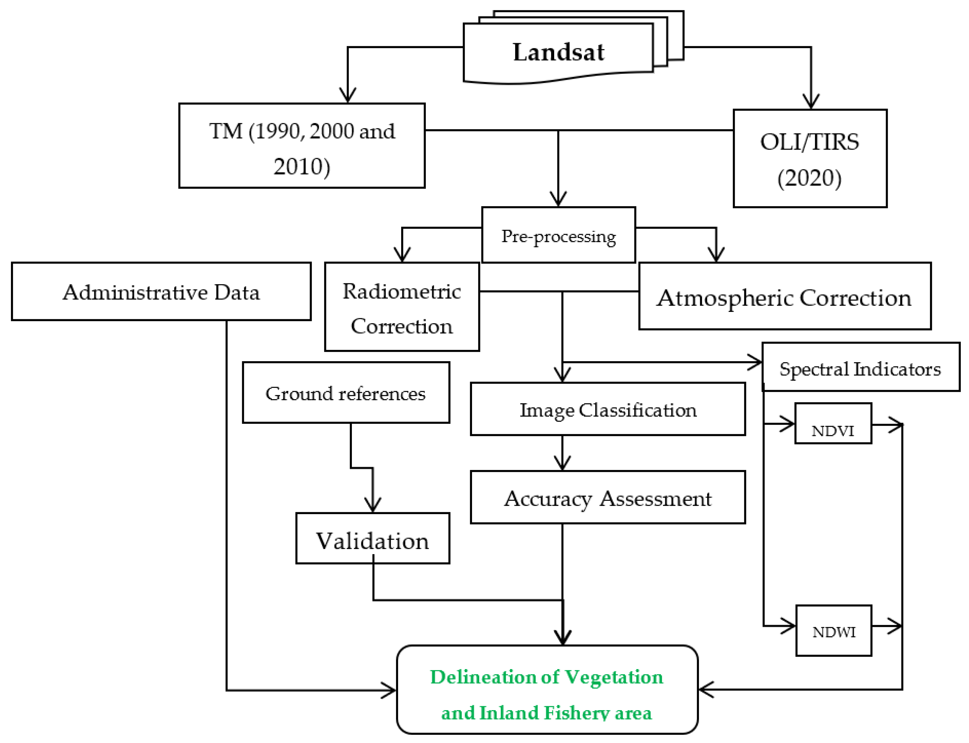
The RS and GIS methods were extensively used for the LU/LC classification and identifying the land area alteration and monitoring the changes and environmental aspects. The Landsat 5 TM and 8 OLI/TIRS datasets for different years were used for mapping the LU/LC classification of the southern parts of North 24 Parganas. The Normalized Different Water Index (NDWI) and the Normalized Different Vegetation Index (NDVI) were used for monitoring the water and vegetation covered area of the study region. The foremost impartial objectives of this study were to: (i) make the LU/LC classification for different years 1990, 2000, 2010, and 2020; (ii) conduct land alteration analysis for different time periods; (iii) identify cropland dynamics and development of inland fishery areas using field data and classification maps; (iv) conduct vegetation and water condition analysis use two different geospatial indicators. The study results will be helpful for local planners, administrative departments like the agricultural department, inland fishery department, policymaker, researchers, and other stakeholders aimed at the development of this study blocks.

2. Study Area

The North 24 Parganas district is situated in West Bengal, which state is located in the eastern portion of India, and the study blocks are in the tropical zone from latitude 22°11′6″ to 23°15′2″ North, and longitude 88°20′ to 89°5′ East. The western parts are in the Kolkata, Howrah, and Hooghly districts. The total area of North 24 Parganas is 4094 km2 and the total population of this district is 10,009,781 (Census of India and North 24 Parganas District handbook, 2011, https://www.census2011.co.in/census/district/11-north-twenty-four-parganas.html (accessed on 23 February 2022)). The headquarters of North 24 Parganas is located at Barasat. The annual average precipitation, or rainfall, is 1550 to 1600 mm. The main urban areas are Barasat, Habra, Madhyamgram, Basirhat, Rajarhat-Newtown, Hasnabad, Dum Dum etc. The average temperatures of this district are 41 °C in the month of May and 10 °C in the month of January, and the relative humidity varies from 50% in the month of March to 90% in the month of July in each year (http://imdkolkata.gov.in/districts/north-24-parganas (accessed on 28 February 2022), Indian Methodological Department, India).
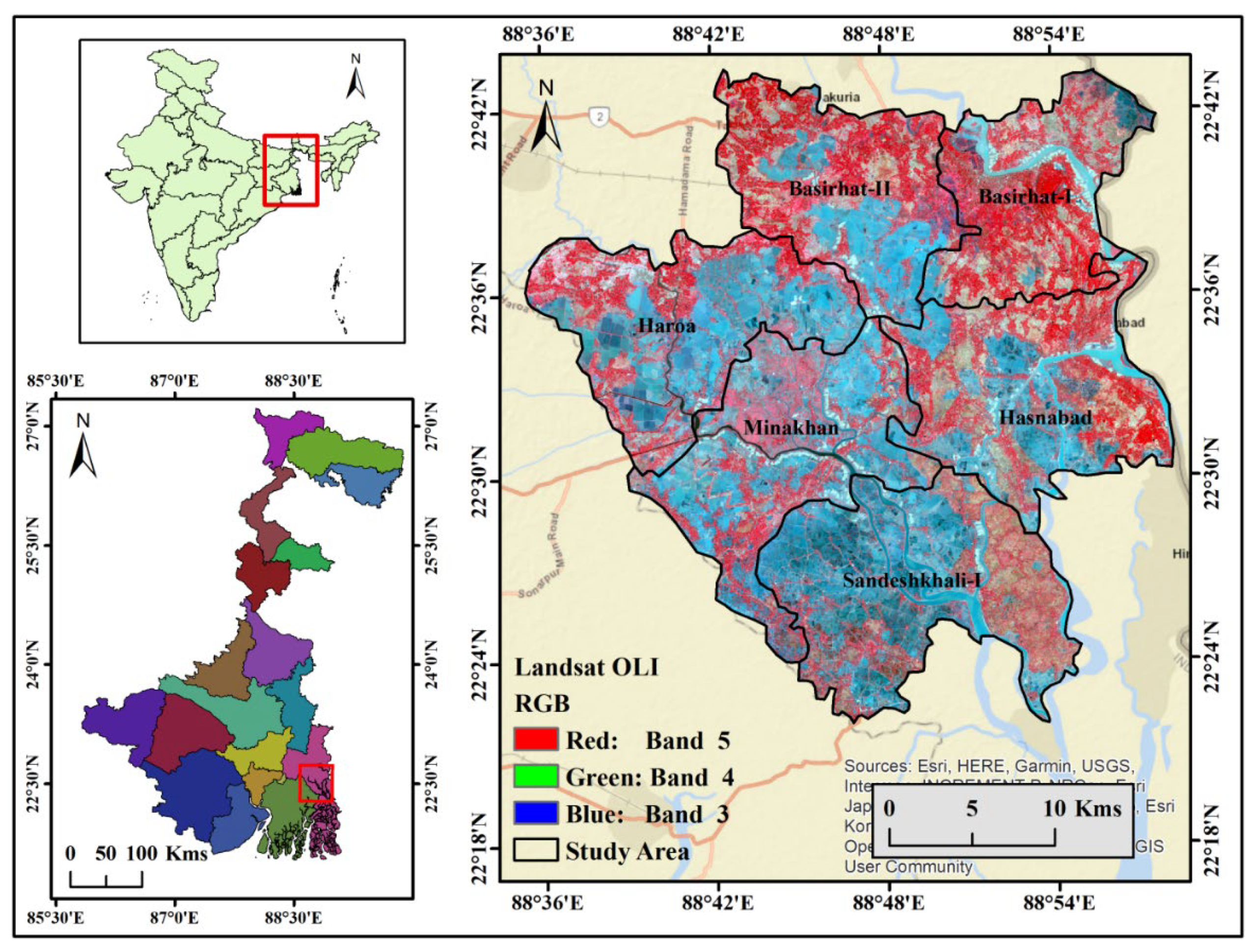
In this study identifying of the area of crop land vulnerability and the area of the inland fishery, six blocks of the North 24 Parganas district were used (there are 22 blocks in the North 24 Parganas district) and the names of those blocks are Haroa, Minakhan, Sandeshkhali-I, Hasnabad, Basirhat-I, and Basirhat-II. Those areas were taken for this study because crop land has been converted into inland fishery in those areas. In the thirty years 1990 to 2020, many crop lands have been converted into brackish water inland fishery use. Gradually, food scarcity has increased due to crop production losses. Farmers are economically building a strong position (http://north24parganas.gov.in/blocks/gaighata/schemes (accessed on 3 March 2022)); however, the land use and land cover (LU/LC) change has been the main reason for crop vulnerability in this study area. The total study area was 927.55 km2 (Figure 1) and it is situated in the southern parts of North 24 Parganas district. The study blocks of North 24 Parganas district are located in the Ganga-Brahmaputra-Meghna delta where extreme environmental events and ecological disturbances have been observed like floods, super cyclones, and manmade disasters. Those climatic conditions are the reason for saltwater intrusion. Saltwater intrusion is the main reason for land use and land cover change and cropland vulnerability. The salt water from the Bay of Bengal has inundated the riverine area and the crop lands are affected by this natural phenomenon. After super cyclone Aila, these areas were affected by saltwater creating huge soil fertility loss related problems. After that, the local farmers, or agriculturalists, have gradually converted the cropland area into inland fisheries.

3. Materials and Method

The water body and cropland dynamics were significantly influenced by the local natural conservation situation and the reserve parts were identified in the study blocks (Figure 2). The areas of inland fishery were increased gradually as the croplands were decreased due to extreme environmental condition and climatic phenomenon in the study area.

3.1. Data Used

Four Landsat 5 Thematic Mapper (TM) and 8 Operational Land Imager/Thermal Infrared Sensor (OLI/TIRS) datasets were used for mapping and monitoring the land dynamic and cropland dynamic in southern selected blocks of North 24 Parganas. The Landsat multi-temporal satellite datasets with less than 10% cloud cover were downloaded from the USGS earth explorer website (https://earthexplorer.usgs.gov/ (accessed on 2 February 2022)). Table 1 shows the sensor, path, row, and data details of different years. The 1990, 2000, 2010 and 2020 Landsat data were used for cropland dynamic and inland fishery area identification over the southern blocks of North 24 Parganas. The administrative boundary of each block and the population data were obtained from Census of India (https://censusindia.gov.in/ (accessed on 5 February 2022)). The ArcGIS 10.4 software (ESRI, Redlands, CA, USA)was used for image classification and monitoring of the inland fishery and cropland situation.

3.2. Satellite Data Pre-Processing

The main objective of this study was to analyse the land alteration due to natural extreme environmental events and climate change. The Landsat data for the four years 1990, 2000, 2010, and 2020 were used for mapping and monitoring the LU/LC change. The satellite datasets were obtained from the earth explorer (USGS website) with minimal alteration in geometric accuracy. The pre-processing of satellite datasets is necessary for LU/LC classification, mapping, and monitoring land dynamic and others earth surface-related work [45]. Geometric correction, atmospheric correction, and radiometric correction are needed for image classification. The ERDAS Imagine version 14 software was used for band combination or layer stacking or band composition, geo-referencing or rectification, masking, and sub-setting or clipping the Area of Interest (AOI). Histogram equalization was used for the enhancement and development of satellite images [46].

3.3. Image Classification and Post Classification

The LU/LC classification of the earth’s surface is the main way to capture the impact of humans on the environment. The ecological balance and environmental conditions are important aspects of our earth’s surface. But the urban expansion, overwhelming population pressure, and hazards such as natural extreme events like cyclones and floods, have influenced the local climatic disorder and environmental degradation [47]. The physical parts like, vegetation, water, soil, and other features have been destroyed by anthropogenic activities. Digital image classification techniques were used for the LU/LC classification [48]. The supervised classification technique with a maximum likelihood algorithm was used for the LU/LC maps classification [49,50]. Land cover was categorised as vegetation area, water bodies, agricultural land, and forest area. Land use/land cover change analysis was used for mapping and monitoring the land dynamic or alteration during the different time periods [51]. After the LU/LC classification, the change detection analysis, accuracy assessment, and the kappa coefficient estimation were the main aspects of the study. The selected blocks of the North 24 Parganas were classified into four classes, agricultural land, water body, vegetation land, and built-up area.
After land use/land cover classification, maps were subjected to an accuracy assessment. The kappa coefficient identification (Table 2) was used for monitoring the error matrix of LU/LC classification [52]. The ERDAS Imagine version 14 software was used for the accuracy assessment and the kappa coefficient. The accuracy valuation of each classified image was carried out by field survey and the data were obtained from Google Earth software. The accuracy assessment and kappa coefficient were calculated used those formulas (Equations (1) and (2)).
O A = ( i = 1 k n i j n )
K i = ( Observed   accuracy Chance   accuracy ) ( 1   Chance   accuracy )
where, nij is representative of the slanting fundamentals in the error matrix, k is the total number of classes in the land use/land cover classification of the selected parts, n is the total number of samples in the error.

3.4. Validation of the Results

The LU/LC classifications derived from different Landsat images had problems due to the difficulty of identifying the proper area and validating the result. Because Landsat data has 30-m resolution, pixel mixing, and alteration were the main problems when identifying the land transformation. For validation of the classification results and accuracy assessment, 300 Google Earth sample collections were verified, and the classification results and the kappa coefficient scale were used for finding the suitable classification (Table 2). Field datasets were used aimed at validating the imagery classification results. The accuracy assessments were estimated at 90.33%, 90.67%, 88.00%, and 86.67% in the years of 1990, 2000, 2010, and 2020, respectively. The kappa coefficients were estimated as 0.86 (1990), 0.87 (2000), 0.83 (2010), and 0.80 (2020) correspondingly.

3.5. Image-Based Geo-Spatial Indices

3.5.1. Normalized Difference Vegetation Index (NDVI)

The delineation of green area is the major work for understanding the vegetated area and the health of the vegetation. Satellite-based RS data from the Landsat 5 TM and 8 OLI/TIRS datasets were used for vegetation monitoring of this area. Many indicators or methods have been extensively used for delineating the forest land area over the earth’s surface, but the normalized difference vegetation index (NDVI) has been the most used for identifying the vegetation area [50]. The vegetation index (NDVI) map was used to identify the area of vegetation cover and its reduction over different time scales from 1990 to 2020. The following formula (Equation (3)) was used for delineating the NDVI maps using satellite images.
NDVI = ( NIR Red NIR + Red )
where Red was denoting that the red band and the second band NIR represented the near infrared band of satellite images. The NDVI map shows −1 to +1. The 0 to +1 represented the densely green space or vegetation, and low index values (<) represented the other LU/LC classes of the study location.

3.5.2. Normalized Difference Water Index (NDWI)

The Normalized Difference Water Index (NDWI) was firstly established by McFeeters in 1996 to detect surface water bodies such as the pond, wetland, river, and lake, that is, the water body environments, and to express the measurement or documentation of their duration [53]. The NDWI index was estimated for use with the Landsat TM and OLI/TIRS Multi-spectral satellite images and it has been positively used with additional satellite sensors anywhere the magnitude of the water areas are desirable [54]. The NDWI was calculated using the Equation (4):
NDWI = ( Green NIR Green + NIR )
This formula uses the Green band and the NIR, or Near Infrared band, of the Landsat 5 TM and 8 OLI/TIRS satellite images. The NDWI index values more than zero were identified as those parts that were actual water surfaces, while values less than or equivalent to zero represented the other LU/LC classes or surfaces in the selected region. Values of the NDWI were estimated in ArcGIS version 10.4 software.

3.5.3. LU/LC Feature Prediction

The LU/LC is a fluctuating earth’s surface feature which is changing gradually but the prediction of future classes of LU/LC features is an additional problem to contemplate. Numerous approaches have been used for LU/LC features forecast like Cellular Automata (CA), Artificial neural network (ANN), regression techniques and Markov Chain (MC) [55,56]. The QGIS software and the MOLUSCE plugin were used for the LU/LC prediction investigation in the selected blocks of the North 24 Parganas district. The MOLUSCE plugin tool was used for LU/LC features prediction and for various types of LU/LC, NDVI, LST, and NDWI forecast and simulation. The well-known algorithms like CA, multi-criteria decision analysis, ANN, and logistic regression were used for the earth’s surface. The DEM, distance from river, distance from road, domination lands water bodies, other LU/LC classes, and slope (LU/LC prediction) and Normalized Difference Water Index (NDWI), Normalized Difference Vegetation Index (NDVI), Normalized Difference Salinity Index (NDSI), and Normalized Difference Built-up Index (NDBI) were used for land use and land cover prediction. The 1990 and 2020 classification year images were used for forecasting the 2050-year LU/LC of these selected blocks. For approximating the reproduction of the LU/LC classes, the geometry requirements had similar resolution and the same geographic projection system. Using the Cellular Automata-Artificial neural network method (CA-ANN), a forecast was created for this study location.

4. Result and Discussion

Remote sensing-based Landsat datasets were used for this study to identify the cropland dynamic and inland fishery area using land use and land cover classification, field data collection, and geospatial indicators. The NDWI maps were used for delineating water body area and NDVI maps were used for vegetation area monitoring from 1990 to 2020 over the southern parts of North 24 Parganas. Supervised classification techniques with maximum likelihood algorithms were used for the LU/LC classification. The results show that quantifiable values of land alteration occurred during the last thirty years and the LU/LC maps and geospatial indicators (NDVI and NDWI) shows that the alteration of land and the socio-economic values also increased.

4.1. Land Dynamic Analysis

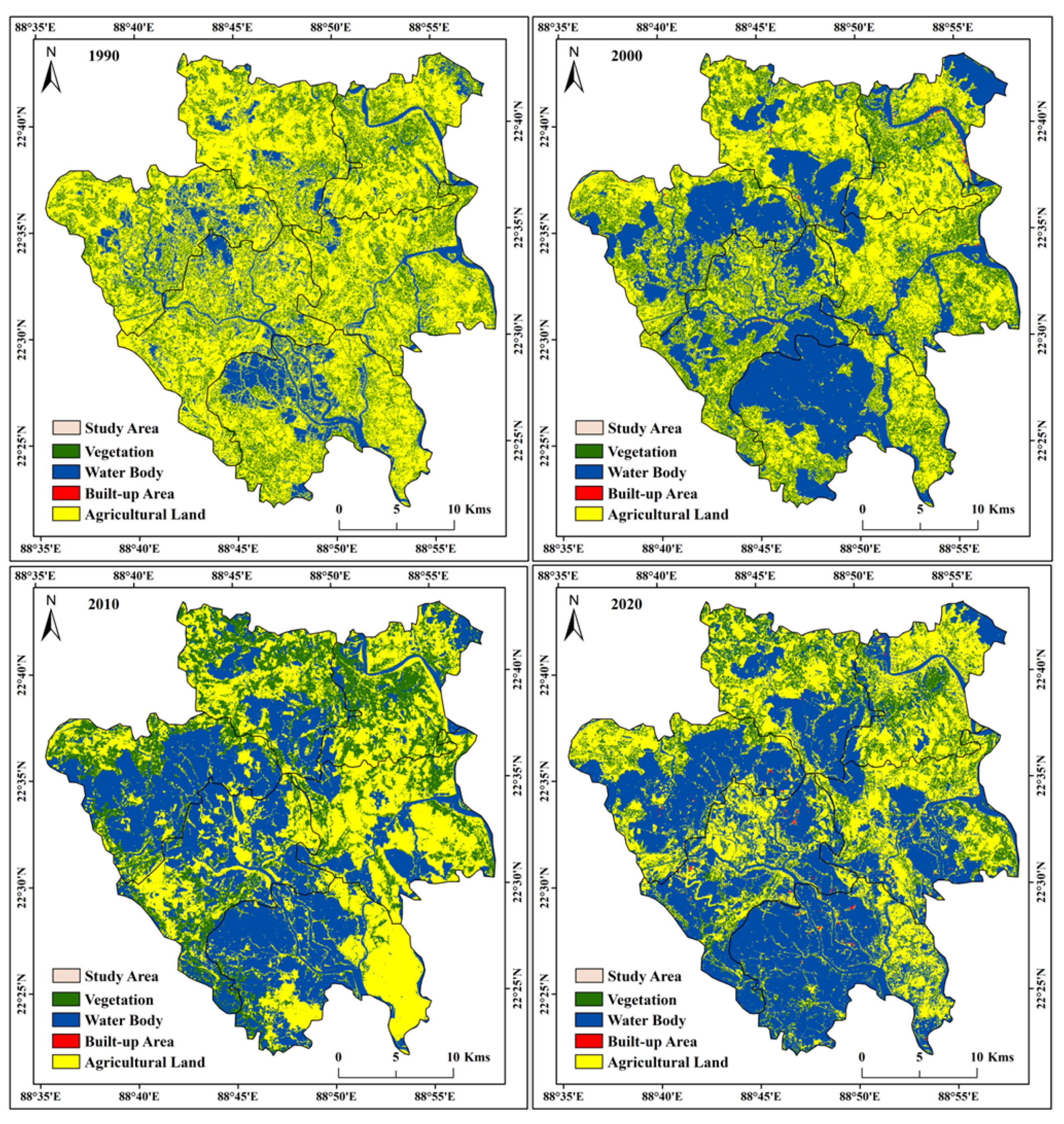
The Landsat 5 TM and 8 OLI/TIRS data of dissimilar years (1990, 2000, 2010, and 2020) were used for this study. A supervised classification technique with maximum likelihood algorithms was used for the LU/LC classification in southern parts of the North 24 Parganas block. Four types of LU/LC classes were identified in this study area, which were built-up land, agricultural land/ cropland water body, and vegetation. The built-up land and water bodies were increased progressively, whereas agricultural land and vegetation areas have been reduced due to several cyclonic floods and extreme environmental conditions over selected blocks of North 24 Parganas. Land transformation is the main occurring result for the LU/LC classification and the LU/LC transformation was augmented by the ecological susceptibility of the study location. The ecosystem was mostly affected by aspects due of land alteration. Agricultural land or croplands were converted into inland fishery areas and the riverine areas were mostly affected by several extreme natural events (Table 3 and Table 4).
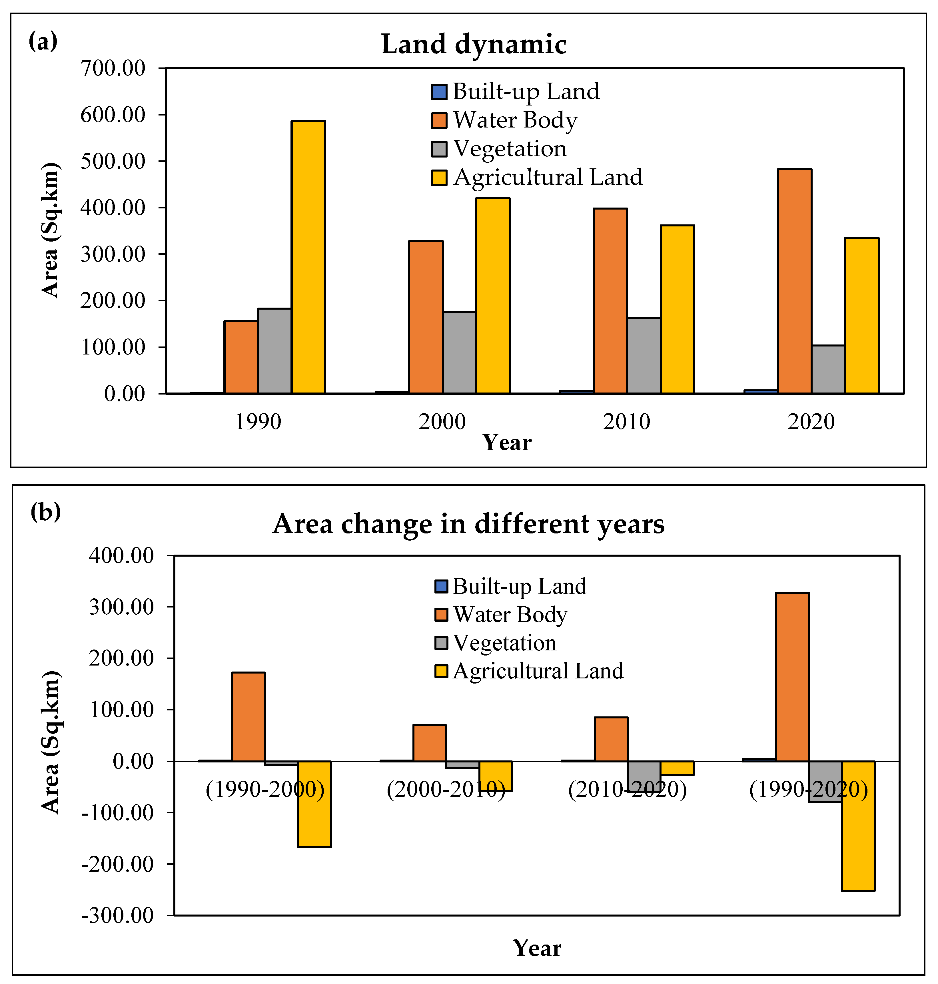
The area of built-up lands in the four years were 2.23 km2 (1990), 3.75 km2 (2000), 5.43 km2 (2010), and 6.86 km2 (2020). The areas of built-up land were mainly located in the Rampur, Sorberia, Basirhat, Hasnabad, Rameswarpur, Taki, and Haroa areas. Basically, area of built-up lands became less in the study area. Areas of croplands and inland fishery mostly fluctuated in the terms of the land use classes in the study blocks (Table 3). Vegetation land area also decreased due to anthropogenic activities and natural extreme events over the study area. Basirhat-I and Basirhat-II were the two blocks most vegetated in the year 1990, but after that, the vegetation area decreased (Figure 3). A total area of 1852.61 km2 (19.69%) of vegetation land was identified in the year 1990, but after that vegetation area was gradually decreased, as shown by the LU/LC classification results of 175.74 km2 (2000), 162.69 km2 (17.54%), and 103.46 km2 (11.15%) (Figure 3).
The area of agricultural land or croplands identified in the classification maps were 582.52 km2 (63.23%), 419.92 km2 (45.27%), 361.67 km2 (38.99%), and 334.46 km2 (36.06%) in the years 1990, 2000, 2010 and 2020, respectively (
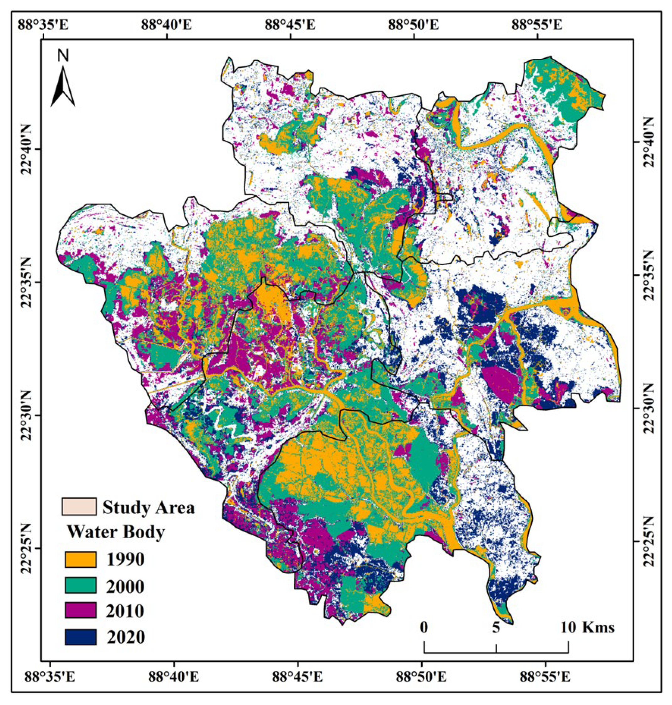
Figure 4a,b). Agricultural cropland was the most affected LU/LC class of this region because of natural extreme events and man-made hazards. The water bodies were mainly river and inland fishery areas. The Landsat data for these four years were used for this study to identify the increased water area over the study area. The bodies of inland fishery areas were located in the Hatgachi, Sandeshkhali, Bayar Mari Abad, Khariat Abad, Sankardaha Abad, Matbari Abad, Bhurkunda, Mallick Gheri, Ramjay Gheri, and Ranigacchi areas. Those areas were mostly converted to inland fishery areas and the local names of those inland fisheries are ‘Bheri’. The water bodies occupied 156.21 km2 (16.84%), 328.15 km2 (35.38%), 397.77 km2 (42.88%), and 482.78 km2 (52.05%) in the years 1990, 2000, 2010, and 2020, respectively.
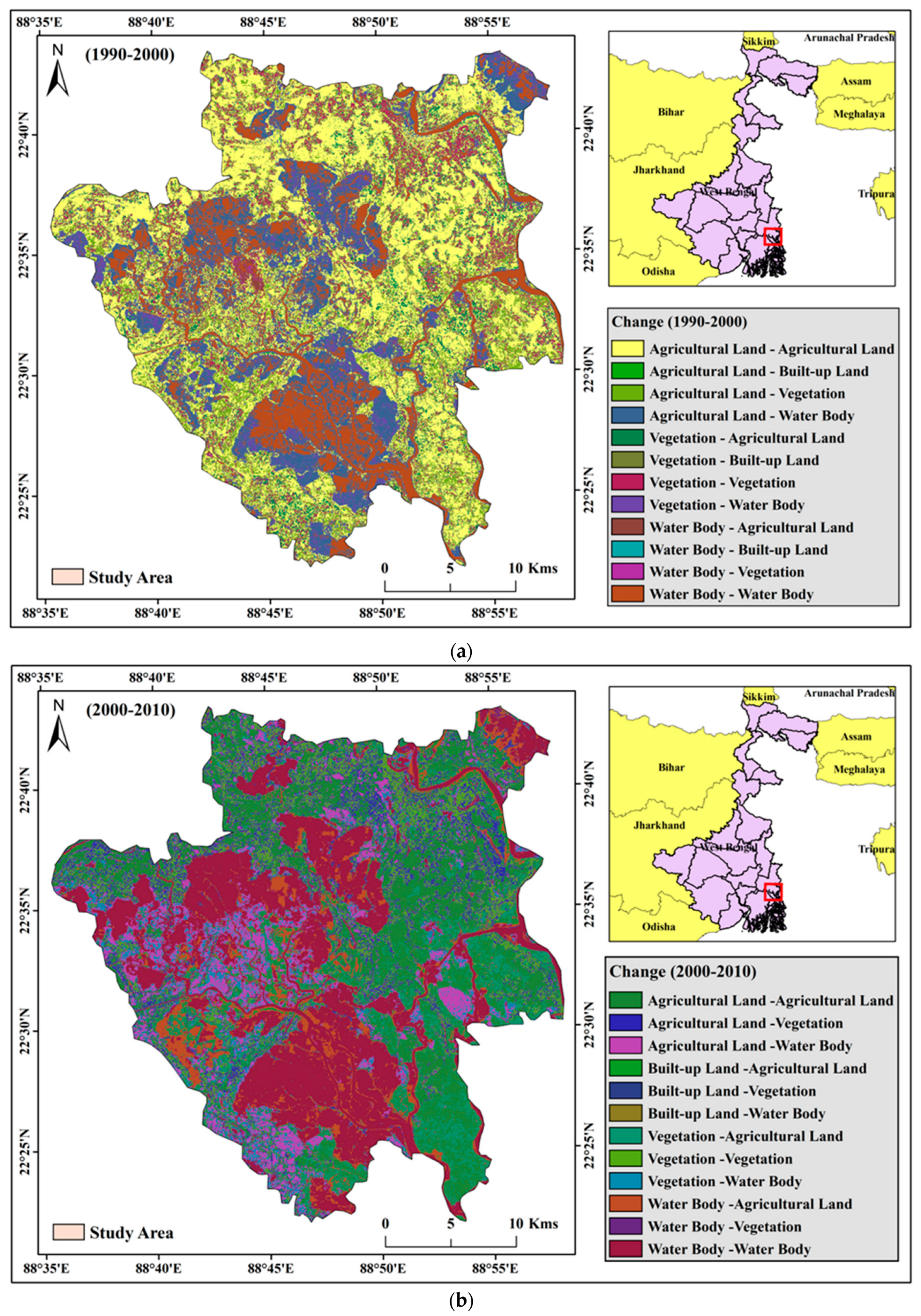
Land alteration or transformation also occurred in the study area and the changed areas for different years were calculated to monitor the yearly land alteration in the study area. From the year 1990 to 2020, the built-up area was increased by 1.52 km2, water body area was increased by 171.94 km2, vegetation and agricultural land were decreased by 6.86 km2 and 166.60 km2, respectively (Table 4). Land-use change and land alteration phenomena are natural conditions, but identification of the reason for land alteration is the most effective way of monitoring the land dynamic [57,58]. From the year 2000 to 2010, the land classes areas were 1.68 km2 for built-up land, 69.62 km2 for water bodies which were increased, and 13.06 km2 for vegetation and 58.25 km2 for agricultural cropland which were both decreased (Figure 5). The same situation was identified by the study area. Many portions of the study area were rehabilitated into the inland fisheries areas due to cyclones and other extreme environmental conditions (
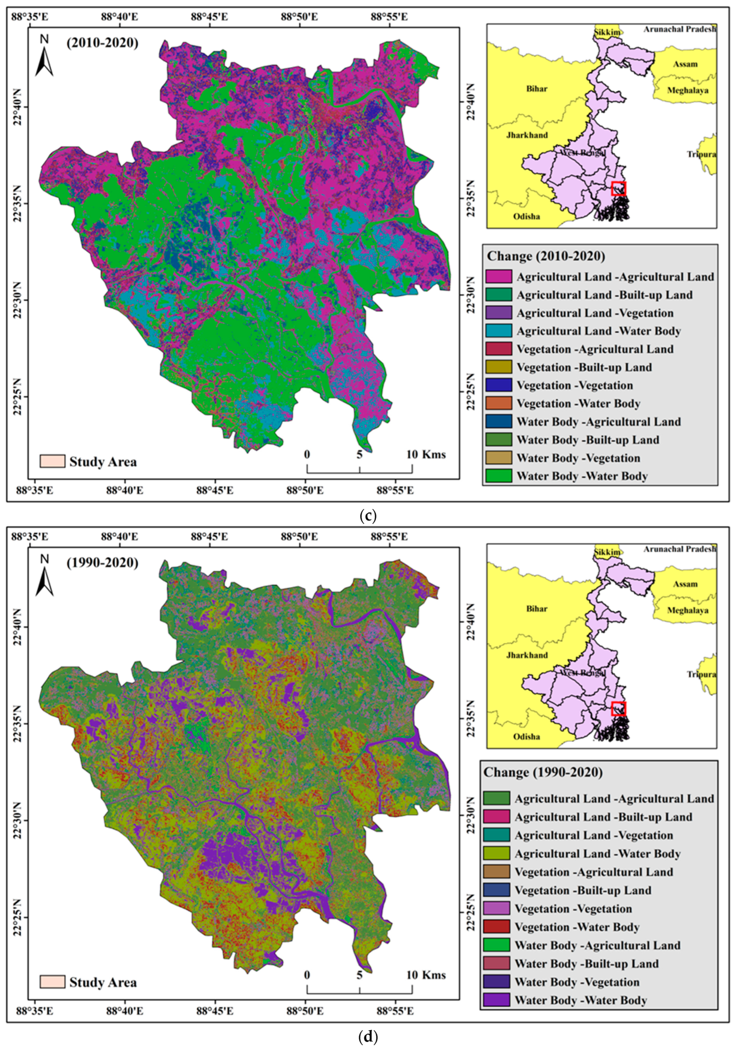
Figure 6). Over the thirty years (1990–2020), the built-up area and water bodies areas were increased 4.63 km2 and 326.58 km2, respectively, also the vegetation and agricultural cropland areas were decreased around 79.15 km2 and 252.06 km2, accordingly (Figure 7a–d). The accuracy assessments were estimated at 90.33%, 90.67%, 88.00%, and 86.67% in the years of 1990, 2000, 2010, and 2020, respectively. The kappa coefficients were identified as 0.86 (1990), 0.87 (2000), 0.83 (2010), and 0.80 (2020), correspondingly (Table 5, Table 6, Table 7 and Table 8).

4.2. Geospatial Indicator

Geospatial indicators have been widely used for delineating the different index-based maps. The Landsat 4–5 TM, 7 ETM+, 8 OLI/TIRS, and Sentinel-2A/B datasets have been used for identification of different geospatial indicators. The most used indicators have been the Normalized Difference Water Index (NDWI), Normalized Difference Vegetation Index (NDVI), Soil-Adjacent Vegetation Index (SAVI), Ratio Vegetation Index (RVI), Transformed Normalized Difference Vegetation Index (TNDVI), Enhance Vegetation Index (EVI), Modified Normalized Difference Water Index (MNDWI), Water Ratio Index (WRI) and Normalized Difference Salinity Index (NDSI) for vegetation, water body, and salinity identification of an area. This study used two geospatial indicators (NDVI and NDWI) for delineating the vegetation scenario and water area identification. Moreover, the indices were used for the validation of the classification. Agricultural land and water area, mainly the area of inland fishery, dominated land classes of the southern parts of North 24 Parganas.
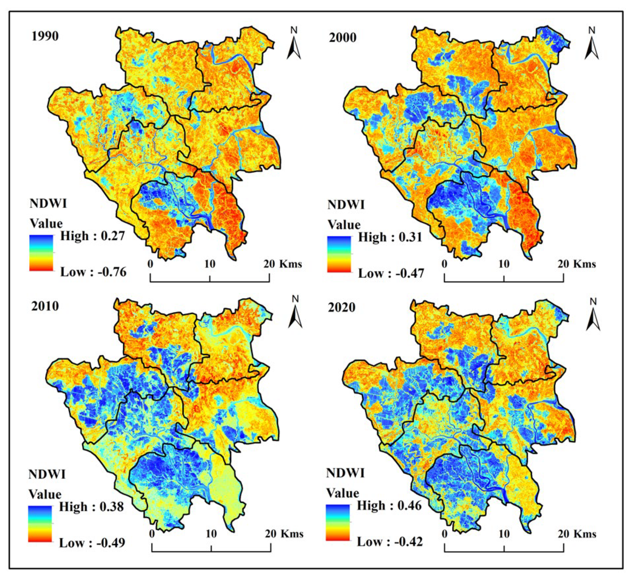
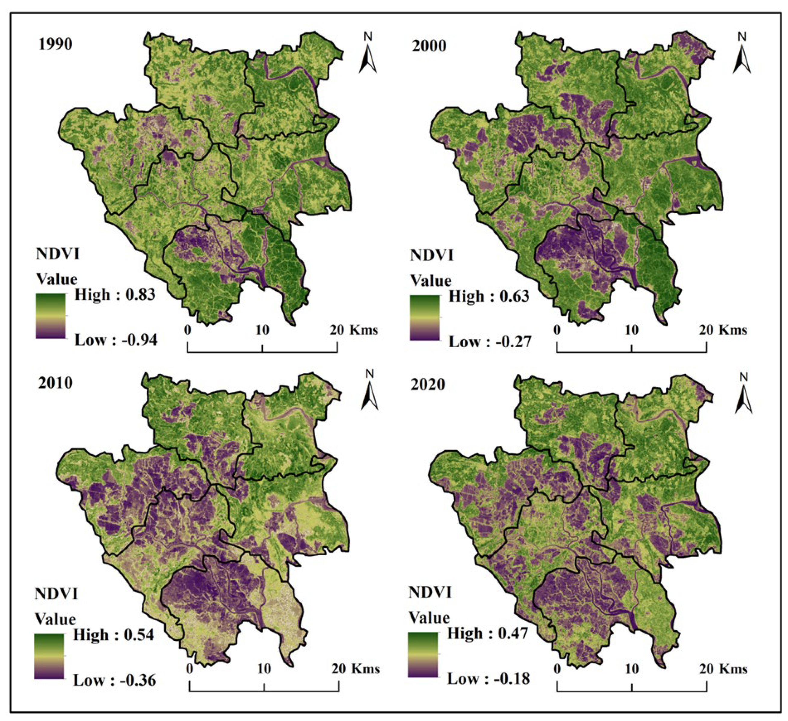
 Figure 8 and Figure 9 show that the NDVI and NDWI maps for different time periods of the southern parts of North 24 Parganas. In the year 1990, the vegetation area occupied a huge amount in the south, north and north-east parts of the study area. After that, the green space area was greatly reduced by human modification and saltwater intrusion over the study area. The green colour shows the vegetated area, and the blue colour indicates the water area. The high values of NDVI were 0.83 (1990), 0.63 (2000), 0.54 (2010), and 0.47 (2020). The NDVI maps show that the vegetation area was degraded, and water bodies increased (Figure 8). Normalized Different Water Index (NDWI) maps were used for defining the area of water bodies in the study location. In the initial phase, the areas of water bodies or inland fisheries, were less and only showed in the Sandeshkhali-I and Haroa blocks, but after the saltwater intrusion, extreme environmental conditions, and disaster-related work, those areas had a huge amount of water area change. The highest values of NDWI were, 0.27 (1990), 0.31 (2000), 0.38 (2010), and 0.46 (2020) (Figure 9). The Aila, Fani, Bulbul, Amphan, and Yash cyclones have destroyed the region and similarly, the inland fishery areas were increased.

4.3. Impact of Cropland Dynamic

Crop production is very important for West Bengal because many people are dependent on rice. Rice is the main food in West Bengal, but it was the rice-growing areas that have been converted into inland fishery areas. Farmers are economically well off for cultivating the fish, but the resultant rice scarcity has increased due to loss of crop land. It was mainly the riverine areas that were converted from cropland into inland fishery use. An administrative awareness program, planning and water quality related information and training was given by the government. The number of markets and preservative companies were increased due to inland fish cultivation, but crop production was decreased on this study area. Around 586.52 km2 (63.23%) of agricultural cropland area was identified in the year 1990, and the most cropped production block was Sandeshkhali-I. After several natural disasters and environmental changes, these blocks were almost all converted from cropland to inland fishery area (Figure 7). In 2020, the agricultural cropland was identified 334.46 km2 (36.06%).

4.4. Impact of Inland Fishery Alteration

Inland fisheries are a more profitable use of this area because of food production and the international demand for fish. Mainly the southern parts of North 24 Parganas are farming different shrimp and crabs for their livelihood. The southern parts of the West Bengal and Odisha coast are regularly affected by several cyclones and natural disasters yearly, that is why those areas are mainly facing a huge amount of saltwater intrusion and the associated decreased soil fertility rate and soil pH, which were the most significant parameters for crop production. But this problem has been widely affected over the area. Several natural disasters like the Aila, Fani, Bulbul, Amphan, and Yash cyclones have affected the riverine area and influence the land dynamic. Fish cultivation is more profitable for the farmers, but the overwhelming land alteration has affected the natural environment and the flora and fauna. The ecosystem of the rural areas has been affected by this type of land alteration.
In the year 1990, 156.21 km2 (16.84%) of the land was identified as water bodies, but several years of cyclonic activities changed the areal conditions over the study area. Most of the inland fishery areas were identified in Sandeshkhali-I and Haroa during 1990 (Figure 6). But after that, several cyclones and environmental disasters have affected the area and influenced land alteration. The Sandeshkhali-I block was the most affected area and had the maximum amount of terrestrial land that was rehabilitated cropland altered to inland fisheries lands. In the year 2020, 482.78 km2 (52.05%) area was under water bodies. This change influenced the land alteration and crop area dynamic. People were mostly building their economic development due to fish production and high international demands for fish-related food production, but the land alteration has degraded the local ecology and environment. Mangrove areas are a natural barrier, which protects the land from extreme environmental and natural disasters. Only the Sandeshkhali-II block has some parts of the mangrove area remaining; the rest of the area is not covered by mangrove forest. The reason for floodwater intrusion is that low land areas and the Ganga delta have a huge amount of high tide related problems. During high tides, many land areas are cover by water. The cyclonic condition has triggered this phenomenon and decreased the soil fertility rate.

4.5. Socio-Economic Values due to Land Alteration

The surface water body change analysis and crop vulnerability area identification was the most effective research work for delineating food scarcity and land dynamic identification. Furthermore, the causes of land dynamics and mitigation strategies are more essential for forthcoming development and sustainable expansion of this area. The southern parts of North 24 Parganas are a riverine area, and those six blocks were the most affected by the natural extreme environment. Cyclones Aila, Bulbul, Fani, Amphan, Yash, and many other natural disasters have triggered the changes in the natural environment and reduced local soil fertility. Good soil fertility and soil quality (pH, nitrogen, etc.) are essential for crop production, but the floods have affected that region, and low soil fertility has triggered the conversion of cropland into inland fishery area over the southern parts of North 24 Parganas. Sandeshkhali-I is the most affected block of North 24 Parganas, with most of the land now covered in inland fisheries. In the initial phase or year of this study, 1990, the area did not support this type of inland fishery, but after Aila, those regions were where the cropland was converted into an inland fishery area. The Kanmari, Chunchura, Matbari Abad, Malancha, Kachurhula, Muchikhola, and Ramchakir Gheri zones then supported an enormous quantity of inland fisheries area.
This remote sensing (RS) and geographic information system (GIS) based study has indicated that the land dynamic over thirty years in southern parts of North 24 Parganas has changed. The Landsat 5 TM and 8 OLI/TIRS datasets were used for this study from 1990 to 2020 at 10-year intervals. The NDVI and NDWI geospatial indices were used for green space or vegetation degradation and water area change analysis. The geospatial indicator was widely used for monitoring the land-related study and different NDWI maps for the four years show that the water areas have changed due to climate change and extreme environmental conditions. The Sandeshkhali-I, Haroa, and Minakhan blocks have been most affected by the saltwater interruption because the river areas were situated only on those blocks. This study has identified that the area of cropland has changed, and the inland fishery area has increased, which has developed the local farmer’s economic well-being and they are building their life towards a sustainable healthy livelihood. Government and policymakers also build such type of planning for the overall development of those areas.
West Bengal is the highest rice-producing state of India, but with the overwhelming population pressure and urban expansion towards rural and fringe areas, the areas of cropland and vegetation has decreased. The vegetation area was converted by the local people for building the settlement. The natural extreme environmental conditions and methodological conditions have affected the coastal area, which was the most demanded parts for crop production, by saltwater intrusion and reduced soil fertility rate. But the natural environment and man-made disasters have affected the selected blocks of North 24 Parganas and increased the inland fishery area due to saltwater intrusion. Farmers are mostly economically stronger because of fish production. National and international fish cultivation demands are very high, and farmers have increased their profit by farming fish and crabs. Mainly, the selected blocks of North 24 Parganas were farming brackish water inland fish after conversion of cropland to fishery areas, and farmers were most economically strong and built proper environmental conditions over the study area. The Central Inland Fishery Research Institute (http://www.cifri.res.in/ (accessed on 28 February 2022)), which is situated in Barrackpore, runs an awareness program for farmers, training, and a water quality monitoring centre for the development of fish production, for the general improvement of this study location.

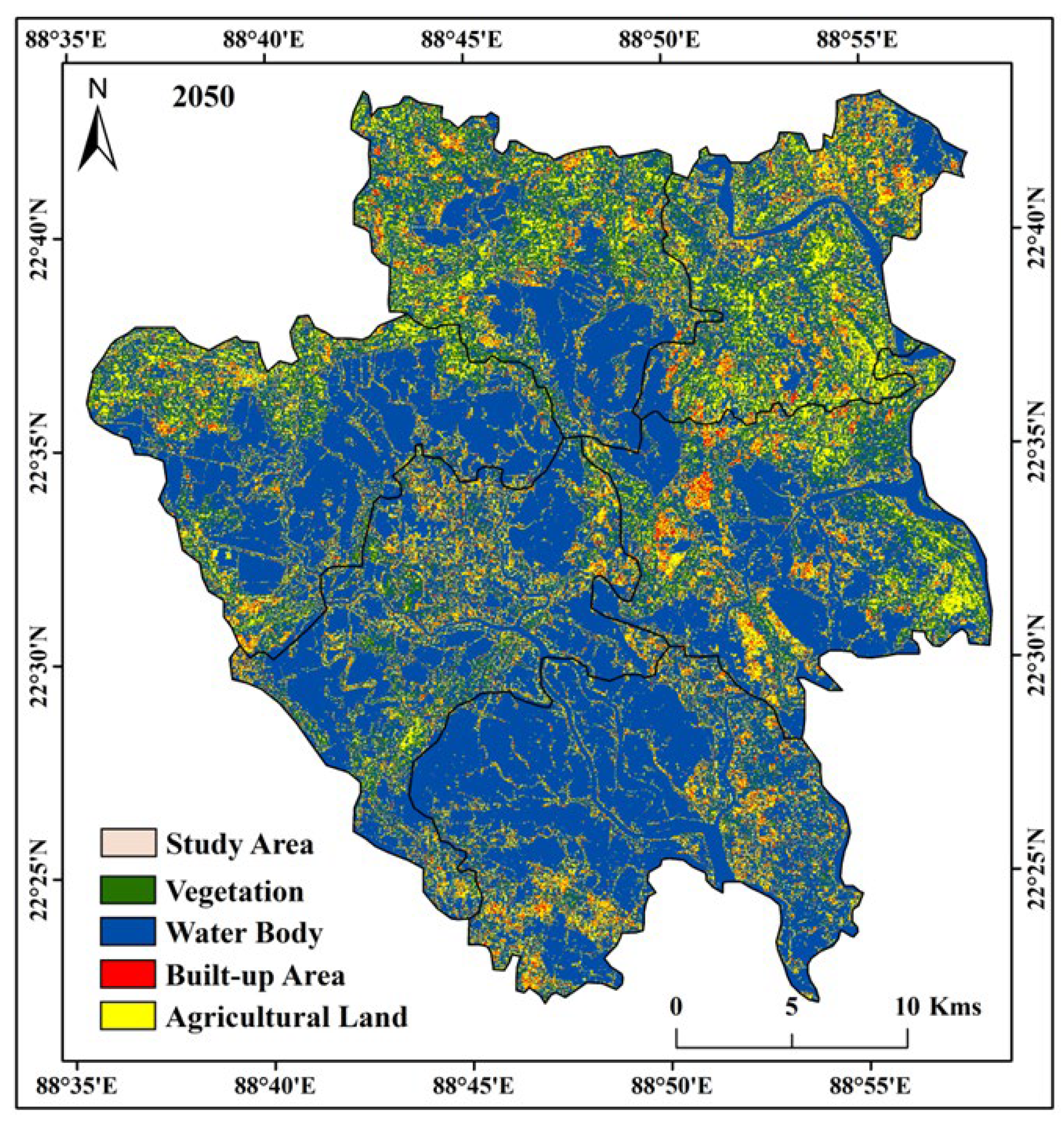
4.6. Land Use/Land Cover Prediction for 2050

For the LU/LC forecast for the year 2050, the two different image classification maps of 1990 and 2020, distance from road and the digital elevation model (DEM) were used with the QGIS software MOLUSCE plugin toolbar or algorithm. The forecast map shows that the natural disaster connected phenomena will augment the agricultural land alteration and control the water bodies or inland fisheries location. The soil salinity of the land and the inland fisheries lands will both be increased in forthcoming years. In the predicted LU/LC map for the year 2050, the water body or inland fishery was identified as 614.73 km2 (66.27%), agricultural land as 217.38 km2 (23.44%), vegetation as 76.85 km2 (8.28%), and built-up land as occupying 18.58 km2 or 2% of the total area (Figure 10). The water bodies or inland fishery area will have increased gradually and the agricultural cropland and vegetation significantly been decreased. Due to urban expansion and overwhelming population pressure, the settlements land will be likewise increased [59]. The reduced agricultural cropland and vegetation land combined with the local climatic disorder will result in a degraded environmental condition. The fishery area will be increased gradually and the area along the river side will be the most affected by this LU/LC change. The Sandeshkhali-I, Minakhan, Haroa and Basirhat-II blocks will be the most affected by 2050.

5. Limitation and Recommendation

The Landsat 5 TM and 8 OLI/TIRS datasets were used for calculating the LU/LC change, then geospatial indicators (NDVI and NDWI) were used for identification in the selected blocks of North 24 Parganas district, West Bengal, India. Four multi-temporal datasets were used for this cropland dynamic and inland fishery area identification (1990, 2000, 2010 and 2020). Due to resolution problems and pixel mixing problems, the area identification was more difficult for and is a limitation of the Landsat data. Additionally, the area of cloud cover and pixel identification were the most important limitations of these images. But the Landsat data have been widely used for earth surface change analysis. The CA-ANN model was used for the LU/LC prediction of the study location [42]. The QGIS software was used for the purpose of the LU/LC prediction, where some of the most significant variables for prediction such as the road density, elevation, slope, and residential areas were used. The CA-ANN model is not used for established designated standards in the structure of each weighting contribution criterion contributing to their significance [60]. The LU/LC did not forecast 100% correctly through several models, therefore better prediction is desirable for future development and management in the study location. This study was also accommodating for the administrators, policymakers, local planners, other stakeholders and researchers for their study and development of this area. The future research scope for this area, are flood susceptibility mapping, soil salinity identification, cropland losses estimation, green space decreased identification, groundwater potential zone and groundwater quality assessment, socio-economic impact study, and improvement of farmers income study.

6. Conclusions

Land dynamics has increased the land scarcity for some areas like urban, peri-urban, and fringe areas, because vegetation and agricultural land has been converted into built-up or industrial land. The North 24 Parganas district is the most land dynamic district of West Bengal because of croplands being converted into inland fisheries due to extreme weather conditions. The Western parts of this district are joint with the megacity Kolkata and the southern parts are mangrove forests. The southern parts of this area have some important rivers, which are the main water source for some time. The Bay of Bengal is situated in the southern part of this area. Every year, the natural environment has been destroyed by the changing climate conditions, floods, cyclones, and many other natural and manmade hazards. This location has been subjected to an enormous volume of saltwater intrusion due to the riverine area that has damaged the cropland over these study areas. The Sandeshkhali, Basirhat, Haroa, Hasnabad, and Minakhan areas are the most affected by natural phenomena and the cyclonic storms that have hammered the natural environment. Due to saltwater intrusion, the land conversion has occurred in the land use and land cover classification map. In 1990, the agricultural land, or mainly the cropland occupied a large area in the selected blocks but after that, the extreme events of climatic change have destroyed the cropland and increased the inland fisheries areas over the study region.
Cropland vulnerability assessment is the most recent work for this study area because most of the people of West Bengal are dependent on rice cultivation and the main food is rice and related items. But the natural cyclones have increased cropland vulnerability over the southern parts of North 24 Parganas. The most affected blocks are the Sandeshkhali-I, Hasnabad, and Haroa. After the super cyclone, Aila, the South, and North 24 Parganas were most affected, and saltwater intrusion has damaged the soil fertility and crop production capacity. The soil is now mostly saline and rice cultivation is not suitable for those areas. Because of this natural climatic condition, many farmers have converted the cropland into brackish water inland fishery areas, resulting in increased crop vulnerability and reduced food security for this location. The cropland area was reduced around 252.06 km2 (1990 to 2020) due to saltwater intrusion and man-made hazards. Gradually the water area was increased by 326.58 km2 (1990 to 2020). Vegetated land area also decreased due to anthropogenic activities and salinity incensement of this area. Around 79.15 km2 of vegetation portions have been lost due to climatic conditions and human activities. There is a need for proper planning, management, and an increased awareness for this problem, and for some mitigation strategies to figure out the sustainable development goals for the study location. Otherwise, saltwater intrusion and land dynamics will increase the crop vulnerability and inland fishery over the study area. The study results can accommodate the policymakers, local administrators, and other stakeholders in building proper planning for those blocks and increasing a better healthy life. Future study is required for the development of this area, such as the identification of areas of flood susceptibility, soil salinity, crop production and fish production, and the socio-economic conditions of this area, and agricultural application. This study method can also be used for future study over some other areas with or without suitable modification.

Author Contributions

Conceptualization, B.H., S.A.A., R.D., M.S. and Z.M.Y.; data curation, B.H., R.D., M.S. and Z.M.Y.; formal analysis, B.H., J.B., H.A.A., M.H.N., S.A.A., K.M.K., K.T.F., R.D., M.S. and Z.M.Y.; investigation, J.B., H.A.A., M.H.N., K.M.K., K.T.F., R.D. and Z.M.Y.; methodology, B.H., M.H.N., K.M.K., K.T.F. and M.S.; project administration, Z.M.Y.; resources, Z.M.Y.; software, B.H.; supervision, K.M.K.; validation, B.H., J.B., M.H.N., S.A.A., R.D. and M.S.; visualization, B.H., J.B., H.A.A., K.T.F., R.D. and Z.M.Y.; writing—original draft, B.H., J.B., H.A.A., M.H.N., S.A.A., K.M.K., K.T.F., R.D., M.S. and Z.M.Y. All authors have read and agreed to the published version of the manuscript.

Funding

This work was financially supported predominantly by WATERAGRI (European Union Horizon 2020 research and innovation programme under Grant Agreement Number 858735).

Data Availability Statement

Data are presented in the article.

Acknowledgments

The first two authors are thankful to the Vidyasagar University for this research opportunity and truly thankful to the local government body for field survey and data collection. This work was supported by the King Khalid University, Abha, Saudi Arabia (by grant number R.G.P. 3/237/43). We express our gratitude to the Deanship of Scientific Research, King Khalid University, for its support of this study.

Conflicts of Interest

The authors declare no conflict of interest.

References

  1. Choudhury, D.; Das, K.; Das, A. Assessment of Land Use Land Cover Changes and Its Impact on Variations of Land Surface Temperature in Asansol-Durgapur Development Region. Egypt. J. Remote Sens. Sp. Sci. 2019, 22, 203–218. [Google Scholar] [CrossRef]
  2. Kumar, D.; Pfeiffer, M.; Gaillard, C.; Langan, L.; Scheiter, S. Climate Change and Elevated CO2 Favor Forest over Savanna under Different Future Scenarios in South Asia. Biogeosciences 2021, 18, 2957–2979. [Google Scholar] [CrossRef]
  3. Siddique, M.A.; Dongyun, L.; Li, P.; Rasool, U.; Khan, T.U.; Farooqi, T.J.A.; Wang, L.; Fan, B.; Rasool, M.A. Assessment and Simulation of Land Use and Land Cover Change Impacts on the Land Surface Temperature of Chaoyang District in Beijing, China. PeerJ 2020, 8, e9115. [Google Scholar] [CrossRef] [PubMed]
  4. Salman, S.A.; Shahid, S.; Sharafati, A.; Salem, G.S.A.; Bakar, A.A.; Farooque, A.A.; Chung, E.-S.; Ahmed, Y.A.; Mikhail, B.; Yaseen, Z.M. Projection of Agricultural Water Stress for Climate Change Scenarios: A Regional Case Study of Iraq. Agriculture 2021, 11, 1288. [Google Scholar] [CrossRef]
  5. Sun, F.; Sun, W.; Chen, J.; Gong, P. Comparison and Improvement of Methods for Identifying Waterbodies in Remotely Sensed Imagery. Int. J. Remote Sens. 2012, 33, 6854–6875. [Google Scholar] [CrossRef]
  6. Meng, X.; Zhang, Y.; Yu, X.; Zhan, J.; Chai, Y.; Critto, A.; Li, Y.; Li, J. Analysis of the Temporal and Spatial Distribution of Lake and Reservoir Water Quality in China and Changes in Its Relationship with GDP from 2005 to 2010. Sustainability 2015, 7, 2000–2027. [Google Scholar] [CrossRef] [Green Version]
  7. Khaleefa, O.; Kamel, A.H. On The Evaluation of Water Quality Index: Case Study of Euphrates River, Iraq. Knowl.-Based Eng. Sci. 2021, 2, 35–43. [Google Scholar] [CrossRef]
  8. Yaseen, Z.M. An Insight into Machine Learning Models Era in Simulating Soil, Water Bodies and Adsorption Heavy Metals: Review, Challenges and Solutions. Chemosphere 2021, 277, 130126. [Google Scholar] [CrossRef]
  9. Tiyasha, T.; Bhagat, S.K.; Fituma, F.; Tung, T.M.; Shahid, S.; Yaseen, Z.M. Dual Water Choices: The Assessment of the Influential Factors on Water Sources Choices Using Unsupervised Machine Learning Market Basket Analysis. IEEE Access 2021, 9, 150532–150544. [Google Scholar] [CrossRef]
  10. Adarsa, J.; Shamina, S.; Arkoprovo, B. Morphological Change Study of Ghoramara Island, Eastern India Using Multi Temporal Satellite Data; International Science Congress Association: Indore, India, 2012. [Google Scholar]
  11. Ghosh, A.; Mukhopadhyay, S. Quantitative Study on Shoreline Changes and Erosion Hazard Assessment: Case Study in Muriganga–Saptamukhi Interfluve, Sundarban, India. Model. Earth Syst. Environ. 2016, 2, 75. [Google Scholar] [CrossRef] [Green Version]
  12. Raju, D.K.; Santosh, K.; Chandrasekar, J.; Tiong-Sa, T. Coastline Change Measurement and Generating Risk Map for the Coast Using Geographic Information System. In Proceedings of the Joint International Conference on Theory, Data Handling and Modelling in GeoSpatial Information Science, Hong Kong, China, 26–28 May 2010. [Google Scholar]
  13. Ghosh, M.K.; Kumar, L.; Roy, C. Monitoring the Coastline Change of Hatiya Island in Bangladesh Using Remote Sensing Techniques. ISPRS J. Photogramm. Remote Sens. 2015, 101, 137–144. [Google Scholar] [CrossRef]
  14. Tao, H.; Al-Bedyry, N.K.; Khedher, K.M.; Shahid, S.; Yaseen, Z.M. River Water Level Prediction in Coastal Catchment Using Hybridized Relevance Vector Machine Model with Improved Grasshopper Optimization. J. Hydrol. 2021, 598, 126477. [Google Scholar] [CrossRef]
  15. Odenweller, J.B.; Johnson, K.I. Crop Identification Using Landsat Temporal-Spectral Profiles. Remote Sens. Environ. 1984, 14, 39–54. [Google Scholar] [CrossRef]
  16. Badhwar, G.D. Automatic Corn-Soybean Classification Using Landsat MSS Data. I. Near-Harvest Crop Proportion Estimation. Remote Sens. Environ. 1984, 14, 15–29. [Google Scholar] [CrossRef]
  17. Bargiel, D. A New Method for Crop Classification Combining Time Series of Radar Images and Crop Phenology Information. Remote Sens. Environ. 2017, 198, 369–383. [Google Scholar] [CrossRef]
  18. Blaes, X.; Vanhalle, L.; Defourny, P. Efficiency of Crop Identification Based on Optical and SAR Image Time Series. Remote Sens. Environ. 2005, 96, 352–365. [Google Scholar] [CrossRef]
  19. Conrad, C.; Dech, S.; Dubovyk, O.; Fritsch, S.; Klein, D.; Löw, F.; Schorcht, G.; Zeidler, J. Derivation of Temporal Windows for Accurate Crop Discrimination in Heterogeneous Croplands of Uzbekistan Using Multitemporal RapidEye Images. Comput. Electron. Agric. 2014, 103, 63–74. [Google Scholar] [CrossRef]
  20. Waldhoff, G.; Lussem, U.; Bareth, G. Multi-Data Approach for Remote Sensing-Based Regional Crop Rotation Mapping: A Case Study for the Rur Catchment, Germany. Int. J. Appl. Earth Obs. Geoinf. 2017, 61, 55–69. [Google Scholar] [CrossRef]
  21. Simonneaux, V.; Duchemin, B.; Helson, D.; Er-Raki, S.; Olioso, A.; Chehbouni, A.G. The Use of High-resolution Image Time Series for Crop Classification and Evapotranspiration Estimate over an Irrigated Area in Central Morocco. Int. J. Remote Sens. 2008, 29, 95–116. [Google Scholar] [CrossRef] [Green Version]
  22. Wardlow, B.; Egbert, S.; Kastens, J. Analysis of Time-Series MODIS 250 m Vegetation Index Data for Crop Classification in the U.S. Central Great Plains. Remote Sens. Environ. 2007, 108, 290–310. [Google Scholar] [CrossRef] [Green Version]
  23. Peña-Barragán, J.M.; Ngugi, M.K.; Plant, R.E.; Six, J. Object-Based Crop Identification Using Multiple Vegetation Indices, Textural Features and Crop Phenology. Remote Sens. Environ. 2011, 115, 1301–1316. [Google Scholar] [CrossRef]
  24. Duro, D.C.; Franklin, S.E.; Dubé, M.G. A Comparison of Pixel-Based and Object-Based Image Analysis with Selected Machine Learning Algorithms for the Classification of Agricultural Landscapes Using SPOT-5 HRG Imagery. Remote Sens. Environ. 2012, 118, 259–272. [Google Scholar] [CrossRef]
  25. Mathur, A.; Foody, G.M. Crop Classification by Support Vector Machine with Intelligently Selected Training Data for an Operational Application. Int. J. Remote Sens. 2008, 29, 2227–2240. [Google Scholar] [CrossRef] [Green Version]
  26. Long, J.A.; Lawrence, R.L.; Greenwood, M.C.; Marshall, L.; Miller, P.R. Object-Oriented Crop Classification Using Multitemporal ETM+ SLC-off Imagery and Random Forest. GIScience Remote Sens. 2013, 50, 418–436. [Google Scholar] [CrossRef]
  27. Siachalou, S.; Mallinis, G.; Tsakiri-Strati, M. A Hidden Markov Models Approach for Crop Classification: Linking Crop Phenology to Time Series of Multi-Sensor Remote Sensing Data. Remote Sens. 2015, 7, 3633–3650. [Google Scholar] [CrossRef] [Green Version]
  28. Behera, M.D.; Prakash, J.; Paramanik, S.; Mudi, S.; Dash, J.; Varghese, R.; Roy, P.S.; Abhilash, P.C.; Gupta, A.K.; Srivastava, P.K. Assessment of Tropical Cyclone Amphan Affected Inundation Areas Using Sentinel-1 Satellite Data. Trop. Ecol. 2022, 63, 9–19. [Google Scholar] [CrossRef]
  29. Halder, B.; Bandyopadhyay, J. Monitoring the Tropical Cyclone ‘Yass’ and ‘Amphan’ Affected Flood Inundation Using Sentinel-1/2 Data and Google Earth Engine. Model. Earth Syst. Environ. 2022, 1–16. [Google Scholar] [CrossRef]
  30. Hassan, M.M.; Ash, K.; Abedin, J.; Paul, B.K.; Southworth, J. A Quantitative Framework for Analyzing Spatial Dynamics of Flood Events: A Case Study of Super Cyclone Amphan. Remote Sens. 2020, 12, 3454. [Google Scholar] [CrossRef]
  31. Halder, B.; Das, S.; Bandyopadhyay, J.; Banik, P. The Deadliest Tropical Cyclone ‘Amphan’: Investigate the Natural Flood Inundation over South 24 Parganas Using Google Earth Engine. Saf. Extrem. Environ. 2021, 3, 63–73. [Google Scholar] [CrossRef]
  32. Bhatta, B.; Saraswati, S.; Bandyopadhyay, D. Urban Sprawl Measurement from Remote Sensing Data. Appl. Geogr. 2010, 30, 731–740. [Google Scholar] [CrossRef]
  33. Belal, A.A.; Moghanm, F.S. Detecting Urban Growth Using Remote Sensing and GIS Techniques in Al Gharbiya Governorate, Egypt. Egypt. J. Remote Sens. Sp. Sci. 2011, 14, 73–79. [Google Scholar] [CrossRef] [Green Version]
  34. Srivastava, A.; Sahoo, B.; Raghuwanshi, N.S.; Singh, R. Evaluation of Variable-Infiltration Capacity Model and MODIS-Terra Satellite-Derived Grid-Scale Evapotranspiration Estimates in a River Basin with Tropical Monsoon-Type Climatology. J. Irrig. Drain. Eng. 2017, 143, 4017028. [Google Scholar] [CrossRef] [Green Version]
  35. MohanRajan, S.N.; Loganathan, A.; Manoharan, P. Survey on Land Use/Land Cover (LU/LC) Change Analysis in Remote Sensing and GIS Environment: Techniques and Challenges. Environ. Sci. Pollut. Res. 2020, 27, 29900–29926. [Google Scholar] [CrossRef] [PubMed]
  36. Mishra, K.; Prasad, P.R.C. Automatic Extraction of Water Bodies from Landsat Imagery Using Perceptron Model. J. Comput. Environ. Sci. 2015, 2015, 903465. [Google Scholar] [CrossRef] [Green Version]
  37. Awadh, S.M.; Al-Sulttani, A.H.; Yaseen, Z.M. Temporal Dynamic Drought Interpretation of Sawa Lake: Case Study Located at the Southern Iraqi Region. Nat. Hazards 2022, 112, 619–638. [Google Scholar] [CrossRef]
  38. Gascon, M.; Cirach, M.; Martínez, D.; Dadvand, P.; Valentín, A.; Plasència, A.; Nieuwenhuijsen, M.J. Normalized Difference Vegetation Index (NDVI) as a Marker of Surrounding Greenness in Epidemiological Studies: The Case of Barcelona City. Urban For. Urban Green. 2016, 19, 88–94. [Google Scholar] [CrossRef]
  39. Hashim, B.M.; Al Maliki, A.; Sultan, M.A.; Shahid, S.; Yaseen, Z.M. Effect of Land Use Land Cover Changes on Land Surface Temperature during 1984–2020: A Case Study of Baghdad City Using Landsat Image. Nat. Hazards 2022, 112, 1223–1246. [Google Scholar] [CrossRef]
  40. McFeeters, S.K. The Use of the Normalized Difference Water Index (NDWI) in the Delineation of Open Water Features. Int. J. Remote Sens. 1996, 17, 1425–1432. [Google Scholar] [CrossRef]
  41. Balzter, H. Markov Chain Models for Vegetation Dynamics. Ecol. Modell. 2000, 126, 139–154. [Google Scholar] [CrossRef] [Green Version]
  42. Santé, I.; García, A.M.; Miranda, D.; Crecente, R. Cellular Automata Models for the Simulation of Real-World Urban Processes: A Review and Analysis. Landsc. Urban Plan. 2010, 96, 108–122. [Google Scholar] [CrossRef]
  43. Zenil, H. Compression-Based Investigation of the Dynamical Properties of Cellular Automata and Other Systems. Complex Syst. 2010, 19, 1–28. [Google Scholar] [CrossRef]
  44. Ménard, A.; Marceau, D.J. Exploration of Spatial Scale Sensitivity in Geographic Cellular Automata. Environ. Plan. B Plan. Des. 2005, 32, 693–714. [Google Scholar] [CrossRef]
  45. Halder, B.; Bandyopadhyay, J.; Banik, P. Assessment of Hospital Sites’ Suitability by Spatial Information Technologies Using AHP and GIS-Based Multi-Criteria Approach of Rajpur–Sonarpur Municipality. Model. Earth Syst. Environ. 2020, 6, 2581–2596. [Google Scholar] [CrossRef]
  46. Meshesha, T.W.; Tripathi, S.K.; Khare, D. Analyses of Land Use and Land Cover Change Dynamics Using GIS and Remote Sensing during 1984 and 2015 in the Beressa Watershed Northern Central Highland of Ethiopia. Model. Earth Syst. Environ. 2016, 2, 1–12. [Google Scholar] [CrossRef] [Green Version]
  47. Halder, B.; Haghbin, M.; Farooque, A.A. An Assessment of Urban Expansion Impacts on Land Transformation of Rajpur-Sonarpur Municipality. Knowl.-Based Eng. Sci. 2021, 2, 34–53. [Google Scholar] [CrossRef]
  48. Shahkooeei, E.; Arekhi, S.; Kani, A.N. Remote Sensing and GIS for Mapping and Monitoring Land Cover and Land Use Changes Using Support Vector Machine Algorithm (Case Study: Ilam Dam Watershed). Int. Res. J. Appl. Basic Sci. 2014, 8, 464–473. [Google Scholar]
  49. Cohen, J.L.; Furtado, J.C.; Barlow, M.; Alexeev, V.A.; Cherry, J.E. Asymmetric Seasonal Temperature Trends. Geophys. Res. Lett. 2012, 39, 1–7. [Google Scholar] [CrossRef]
  50. Halder, B.; Banik, P.; Bandyopadhyay, J. Mapping and Monitoring Land Dynamic Due to Urban Expansion Using Geospatial Techniques on South Kolkata. Saf. Extrem. Environ. 2021, 3, 27–42. [Google Scholar] [CrossRef]
  51. Ramachandra, T.V.; Bharath, S.; Gupta, N. Modelling Landscape Dynamics with LST in Protected Areas of Western Ghats, Karnataka. J. Environ. Manag. 2018, 206, 1253–1262. [Google Scholar] [CrossRef]
  52. Cheruto, M.C.; Kauti, M.K.; Kisangau, P.D.; Kariuki, P. Assessment of Land Use and Land Cover Change Using GIS and Remote Sensing Techniques: A Case Study of Makueni County, Kenya. J. Remote Sens. GIS 2016, 5, 1000175. [Google Scholar] [CrossRef]
  53. McFeeters, S. Using the Normalized Difference Water Index (NDWI) within a Geographic Information System to Detect Swimming Pools for Mosquito Abatement: A Practical Approach. Remote Sens. 2013, 5, 3544–3561. [Google Scholar] [CrossRef] [Green Version]
  54. Chowdary, V.M.; Chandran, R.V.; Neeti, N.; Bothale, R.V.; Srivastava, Y.K.; Ingle, P.; Ramakrishnan, D.; Dutta, D.; Jeyaram, A.; Sharma, J.R.; et al. Assessment of Surface and Sub-Surface Waterlogged Areas in Irrigation Command Areas of Bihar State Using Remote Sensing and GIS. Agric. Water Manag. 2008, 95, 754–766. [Google Scholar] [CrossRef]
  55. Yaseen, Z.M.; Sulaiman, S.O.; Deo, R.C.; Chau, K.-W. An Enhanced Extreme Learning Machine Model for River Flow Forecasting: State-of-the-Art, Practical Applications in Water Resource Engineering Area and Future Research Direction. J. Hydrol. 2018, 569, 387–408. [Google Scholar] [CrossRef]
  56. Yaseen, Z.M.; Shahid, S. Drought Index Prediction Using Data Intelligent Analytic Models: A Review. In Intelligent Data Analytics for Decision-Support Systems in Hazard Mitigation; Springer: Berlin/Heidelberg, Germany, 2020; pp. 1–27. [Google Scholar]
  57. Alsharif, A.A.A.; Pradhan, B. Urban Sprawl Analysis of Tripoli Metropolitan City (Libya) Using Remote Sensing Data and Multivariate Logistic Regression Model. J. Indian Soc. Remote Sens. 2013, 42, 149–163. [Google Scholar] [CrossRef]
  58. Silk, J. Book Reviews: The Restless Urban Landscape; Knox, P., Ed.; Prentice Hall: Englewood Cliffs, NJ, USA, 1993; pp. 9, 285. ISBN 0137554141. [Google Scholar]
  59. Mehr, A.D.; Akdegirmen, O. Estimation of Urban Imperviousness and Its Impacts on Flashfloods in Gazipaşa, Turkey. Knowl.-Based Eng. Sci. 2021, 2, 9–17. [Google Scholar] [CrossRef]
  60. Shatnawi, N.; Qdais, H.A. Mapping Urban Land Surface Temperature Using Remote Sensing Techniques and Artificial Neural Network Modelling. Int. J. Remote Sens. 2019, 40, 3968–3983. [Google Scholar] [CrossRef]
Figure 1. Location map of the selected study area. The red frame shows the identification of the study location.
Agronomy 12 01268 g001
Figure 2. Entire methodology of the study area.
Agronomy 12 01268 g002
Figure 3. Land use and land cover classification maps of different time periods in the study area like 1990, 2000, 2010, and 2020.
Agronomy 12 01268 g003
Figure 4. LU/LC classification area calculation; (a) total LU/LC classes in different time periods; (b) loss/gain analysis of different years.
Agronomy 12 01268 g004
Figure 5. Agricultural Land dynamic in different time periods.
Agronomy 12 01268 g005
Figure 6. Water body change analysis of different study time.
Agronomy 12 01268 g006
Figure 7. Change detection analysis of different time periods. (a) 1990–2000; (b) 2000–2010; (c) 2010–2020; and (d) 1990–2020. The red frame shows the identification of the study location.
Agronomy 12 01268 g007aAgronomy 12 01268 g007b
Figure 8. Normalized Different Vegetation Index (NDVI) maps of the study area.
Agronomy 12 01268 g008
Figure 9. Normalized Difference Water Index (NDWI) maps of the study area.
Agronomy 12 01268 g009
Figure 10. Prediction map of the study area in the year 2050.
Agronomy 12 01268 g010
Table 1. Details of satellite data and acquisition dates.
SatelliteSensorDatePath and RowData Source
Landsat 5TM14 November 1990138,044https://earthexplorer.usgs.gov/ (accessed on 2 February 2022)
9 November 2000138,044
6 February 2010138,044
Landsat 8OLI/TIRS18 December 2020138,044
Table 2. Scale of Kappa coefficient and the strength of agreement.
Sl No.Value of KStrength of Agreement
1<0.20Poor
20.21–0.40Fair
30.41–0.60Moderate
40.61–0.80Good
50.81–1.00Very good
Table 3. LU/LC area change examination.
Class NameArea in Sq. kmArea in Percentage (%)
19902000201020201990200020102020
Built-up Land2.233.755.436.860.240.400.590.74
Water Body156.21328.15397.77482.7816.8435.3842.8852.05
Vegetation182.61175.74162.69103.4619.6918.9517.5411.15
Agricultural Land586.52419.92361.67334.4663.2345.2738.9936.06
Total927.55927.55927.55927.55
Table 4. Loss and gain analysis of the LU/LC classes.
Class NameArea Change (Sq. km)
(1990–2000)(2000–2010)(2010–2020)(1990–2020)
Built-up Land1.521.681.434.63
Water Body171.9469.6285.02326.58
Vegetation−6.86−13.06−59.23−79.15
Agricultural Land−166.60−58.25−27.21−252.06
Table 5. Accuracy assessment and kappa coefficient in the year of 1990.
Class NameGround Truth/ReferencesRow TotalCommission ErrorUser Accuracy
Water BodyAgricultural Land VegetationBuilt-Up Land
Water body68331759.33%90.67%
Agricultural Land 3996211010.00%90.00%
Vegetation269611058.57%91.43%
Built-up Land01181020.00%80.00%
Column Total7310910612300
Omission Error6.85%9.17%9.43%33.33%
Producer Accuracy93.15%90.83%90.57%66.67%
Overall Accuracy90.33% Kappa Coefficient0.86
Bold indicates the variaiton.
Table 6. Accuracy assessment and kappa coefficient in the year of 2000.
Class NameGround Truth/ReferencesRow TotalCommission ErrorUser Accuracy
Water BodyAgricultural Land VegetationBuilt-Up Land
Water body90431988.16%91.84%
Agricultural Land 294511027.84%92.16%
Vegetation15792879.20%90.80%
Built-up Land11291330.77%69.23%
Column Total941048913300
Omission Error4.26%9.62%11.24%30.77%
Producer Accuracy95.74%90.38%88.76%69.23%
Overall Accuracy90.67% Kappa Coefficient0.87
Bold indicates the variaiton.
Table 7. Accuracy assessment and kappa coefficient in the year of 2010.
Class NameGround Truth/ReferencesRow TotalCommission ErrorUser Accuracy
Water BodyAgricultural Land VegetationBuilt-Up Land
Water body10195211713.68%86.32%
Agricultural Land 38242919.89%90.11%
Vegetation346917710.39%89.61%
Built-up Land012121520.00%80.00%
Column Total107968017300
Omission Error5.61%14.58%13.75%29.41%
Producer Accuracy94.39%85.42%86.25%70.59%
Overall Accuracy88.00% Kappa Coefficient0.83
Bold indicates the variaiton.
Table 8. Accuracy assessment and kappa coefficient in the year of 2020.
Class NameGround Truth/ReferencesRow TotalCommission ErrorUser Accuracy
Water BodyAgricultural Land VegetationBuilt-Up Land
Water body11567112910.85%89.15%
Agricultural Land 673428514.12%85.88%
Vegetation365916914.49%85.51%
Built-up Land301131723.53%76.47%
Column Total127857117300
Omission Error9.45%14.12%16.90%23.53%
Producer Accuracy90.55%85.88%83.10%76.47%
Overall Accuracy86.67% Kappa Coefficient0.80
Bold indicates the variaiton.
Publisher’s Note: MDPI stays neutral with regard to jurisdictional claims in published maps and institutional affiliations.

