
The Quantitative Features Analysis of the Nonlinear Model of Crop Production by Hybrid Soft Computing Paradigm


Abstract
1. Introduction
- Nonlocal strategies are used to approximate nonlinear terms in continuous systems.
- We use the developed nonlinear computational model [8] to determine the effects of insecticides, insects, and external efforts on agricultural crop production in order to achieve optimal crop production.
- Using artificial neural networks, a Levenberg–Marquardt technique (LMT) trains hidden neurons and validates the reference data set obtained using the “NDSolve” tool in Mathematica for different insecticide spraying rates instances.
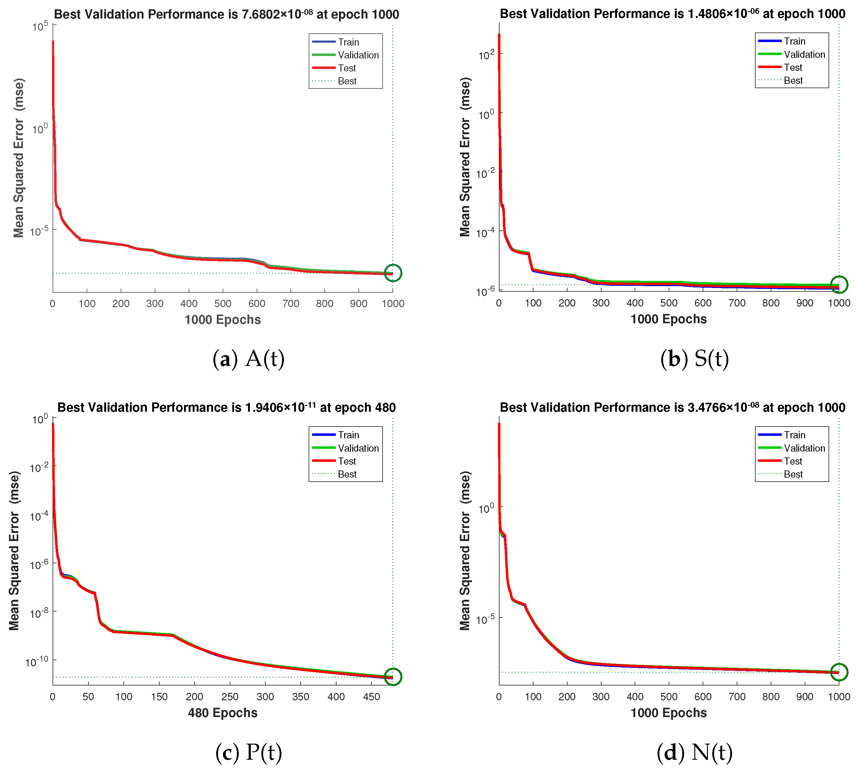
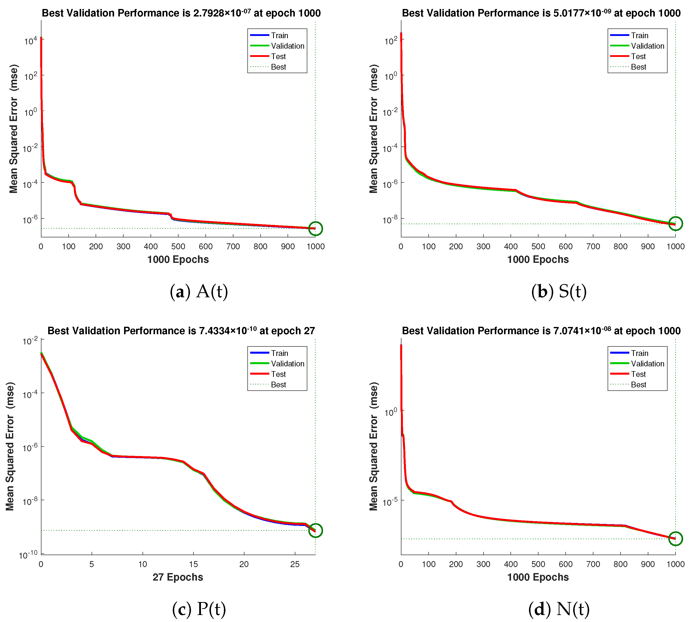
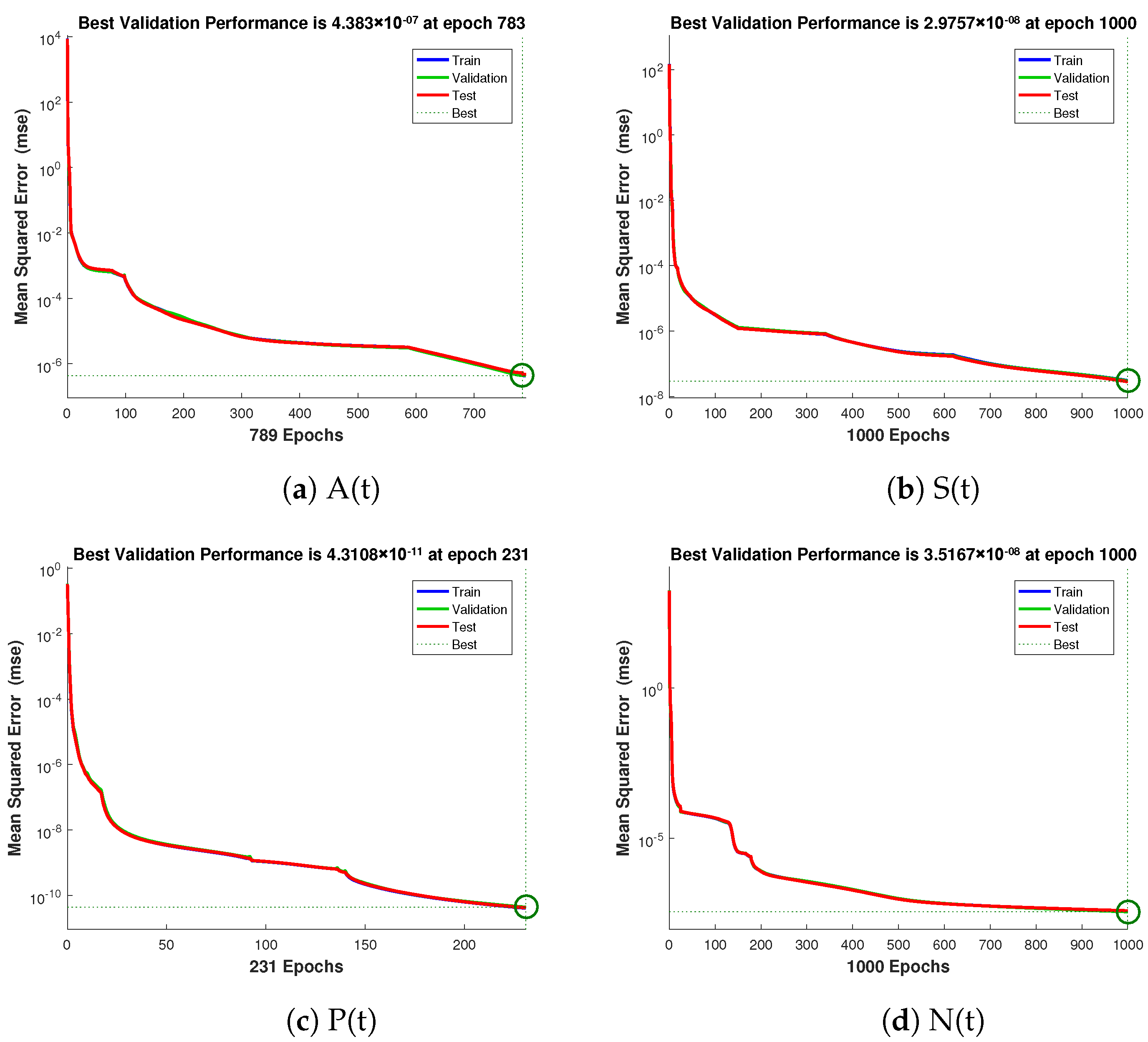
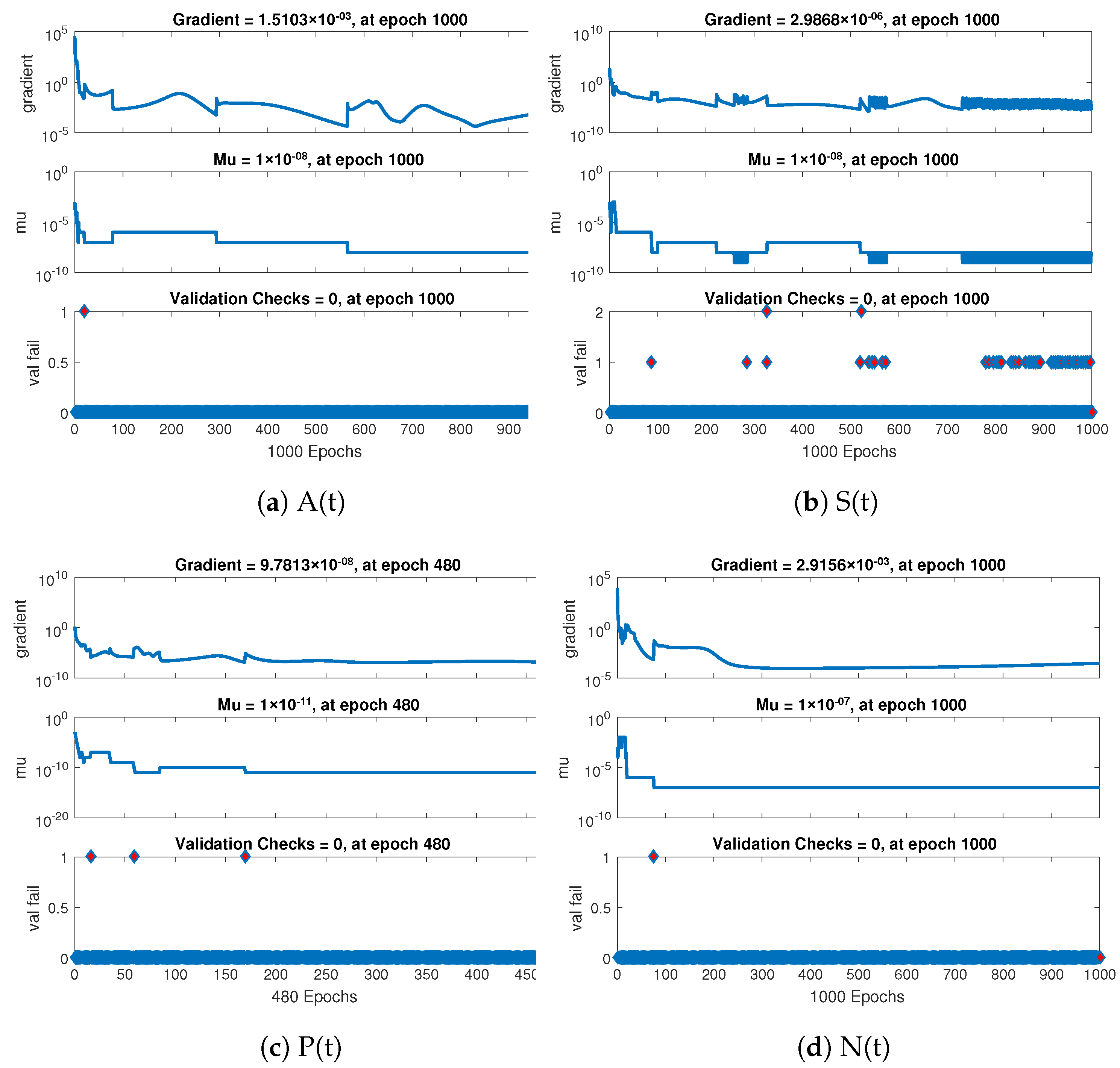
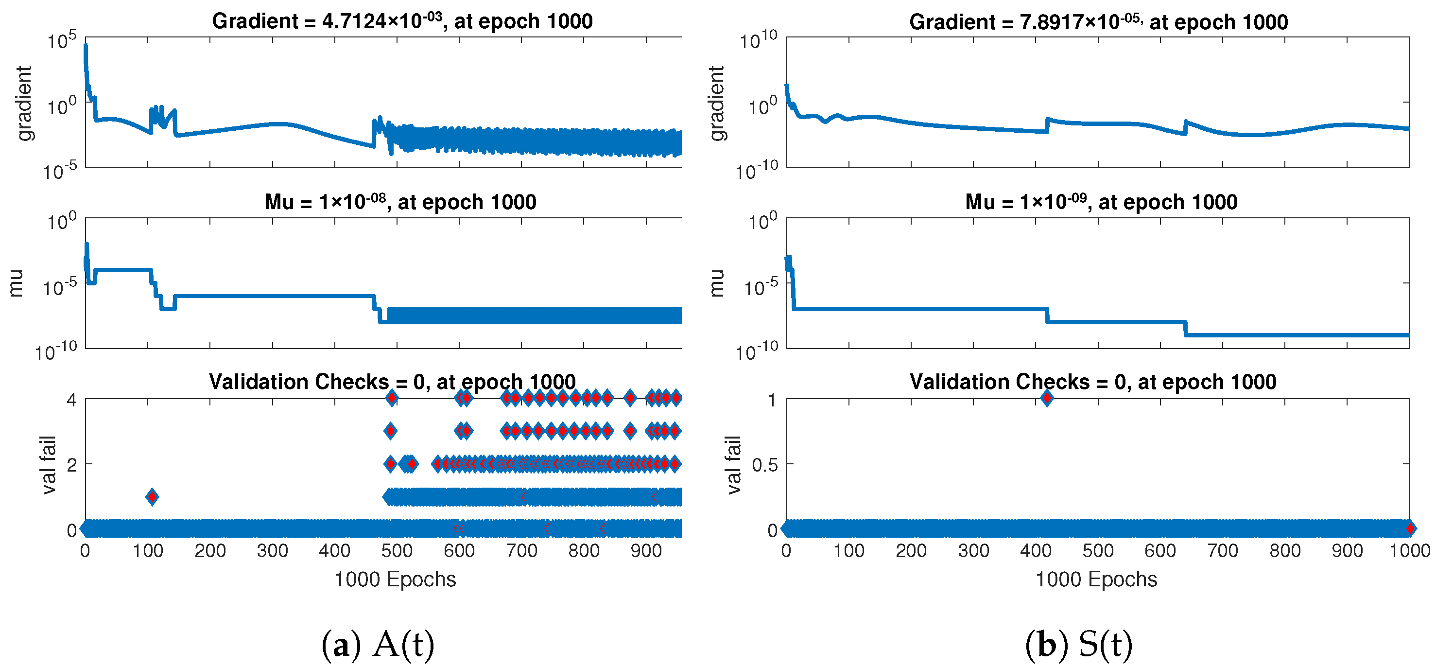
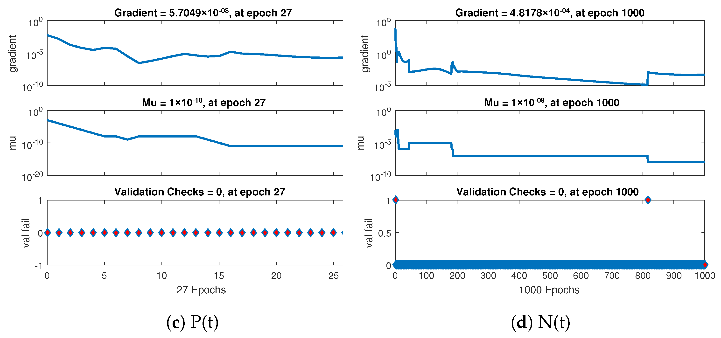
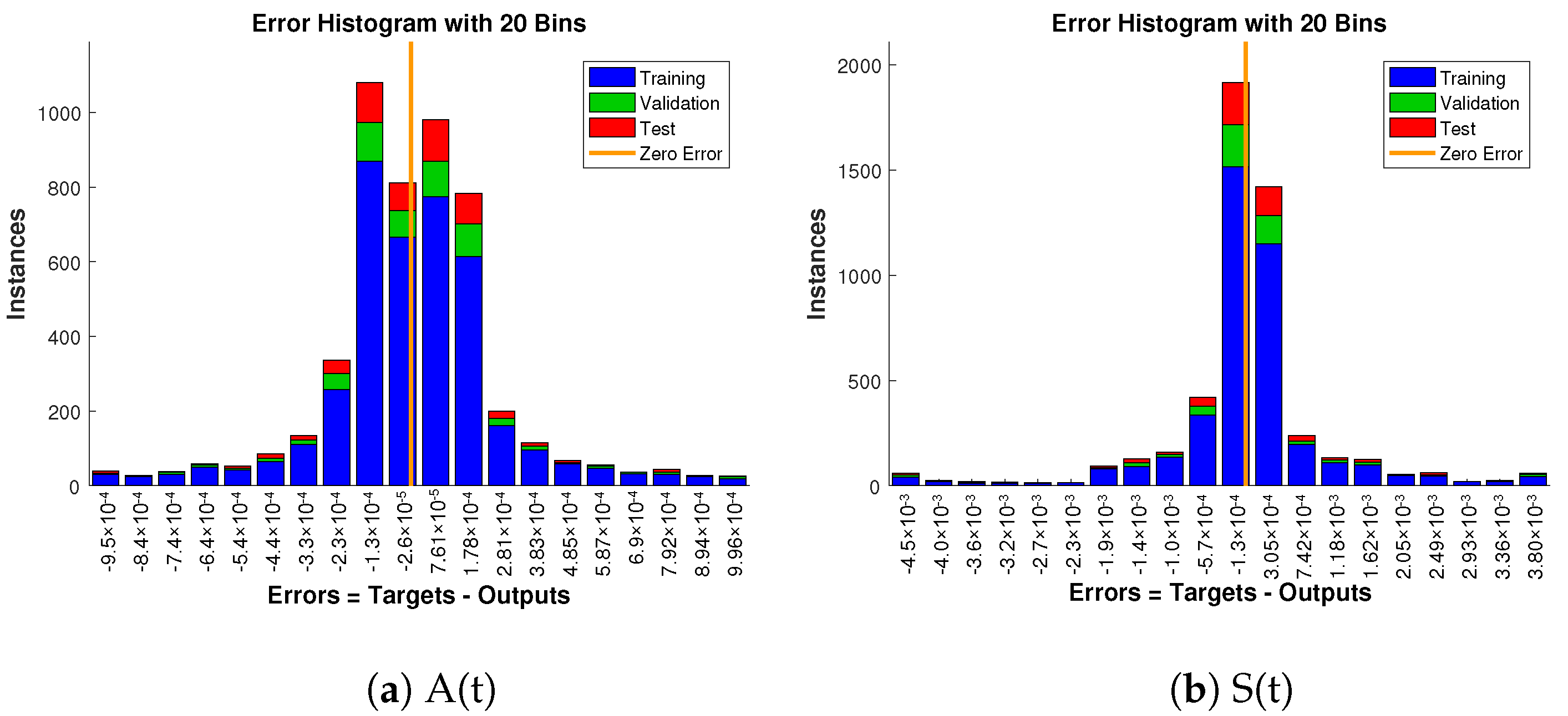
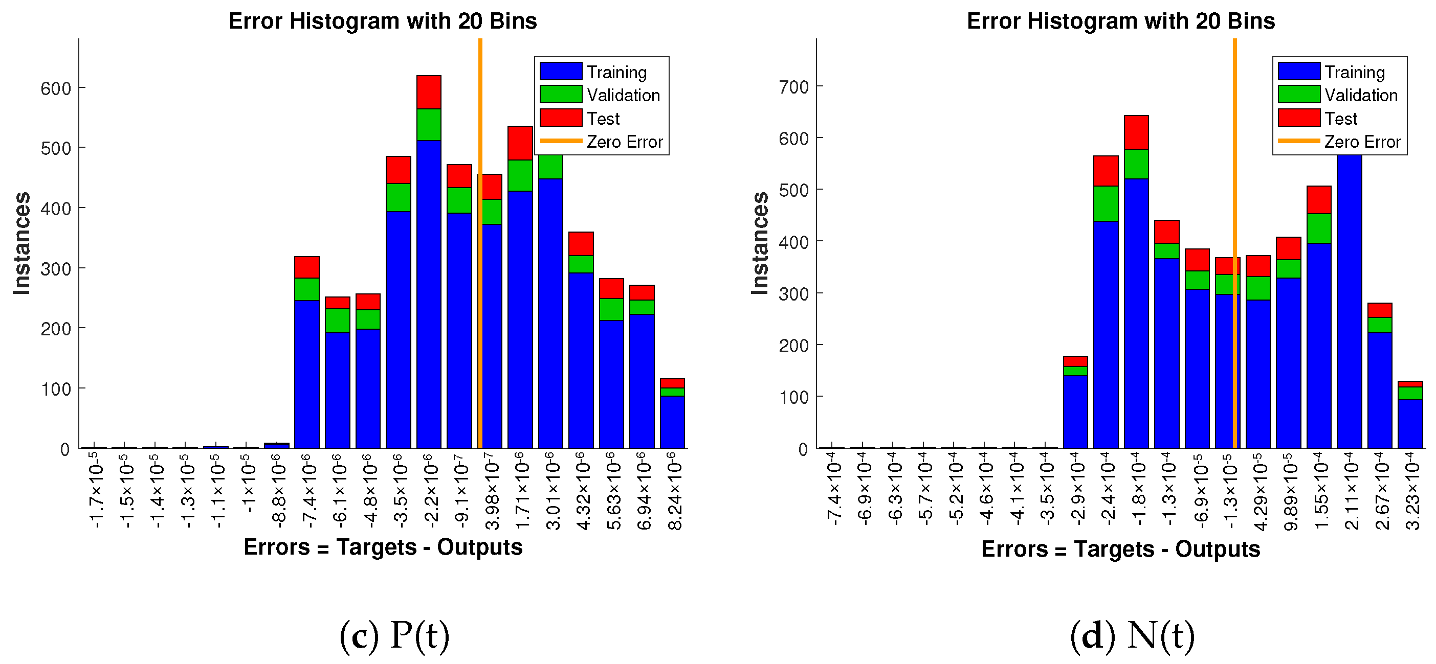
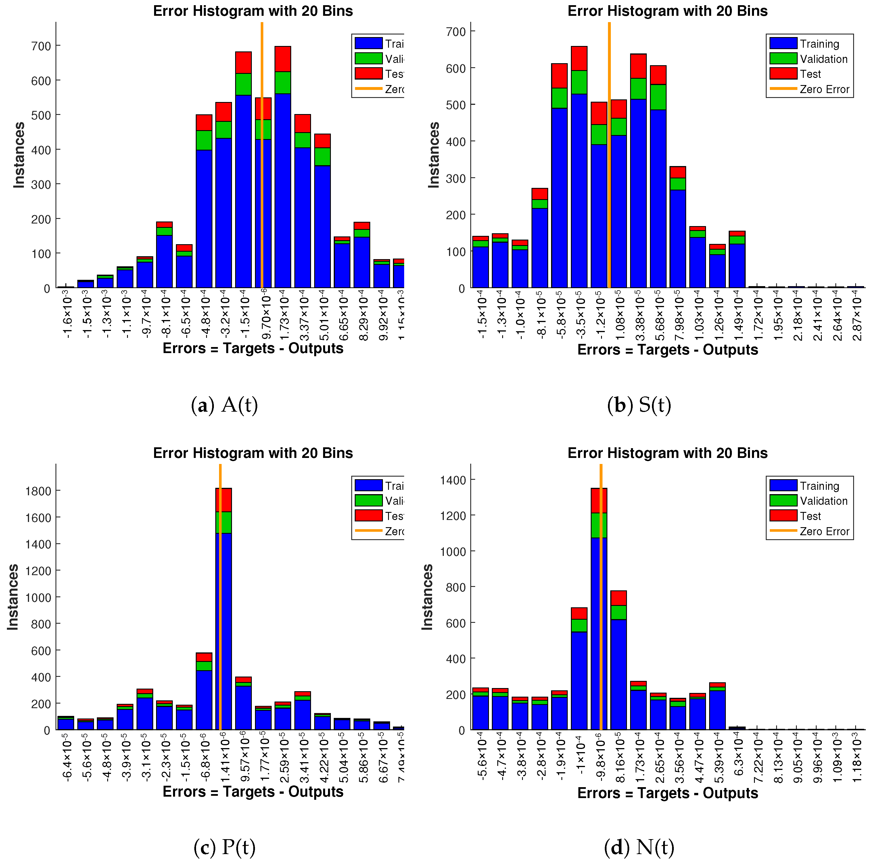
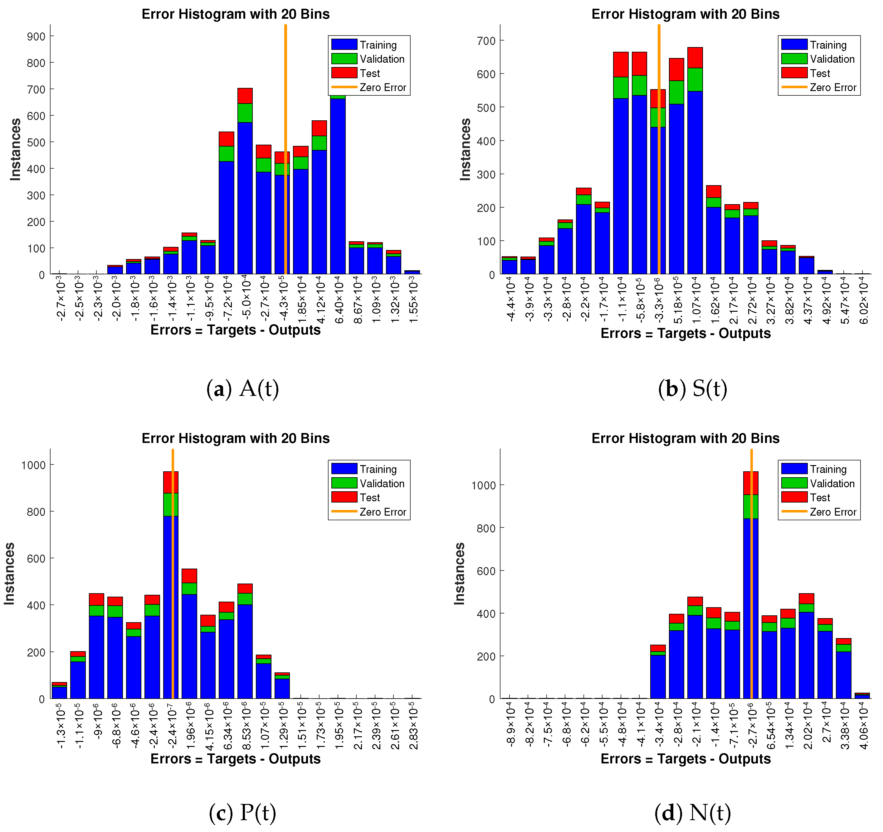
- Based on curve fitting, regression, the mean squared error (MSE), and total and absolute errors, the technique has to prove its convergence, accuracy, and processing cost through extensive graphical study.
2. Problem Formulation
3. Design Methodology
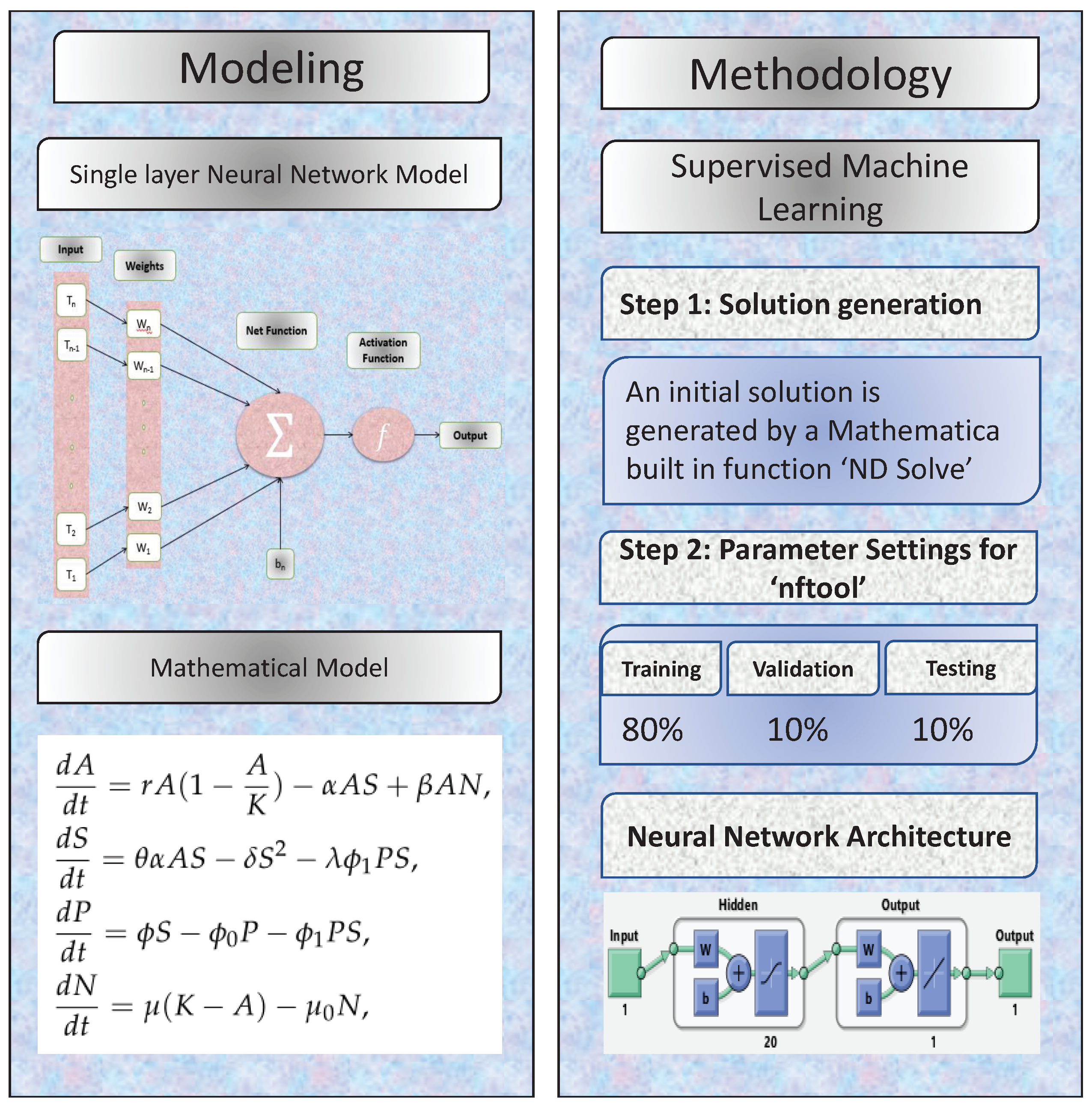
- The “NDSolve” function in Mathematica is used to solve the model (1) numerically for the initial data collection.
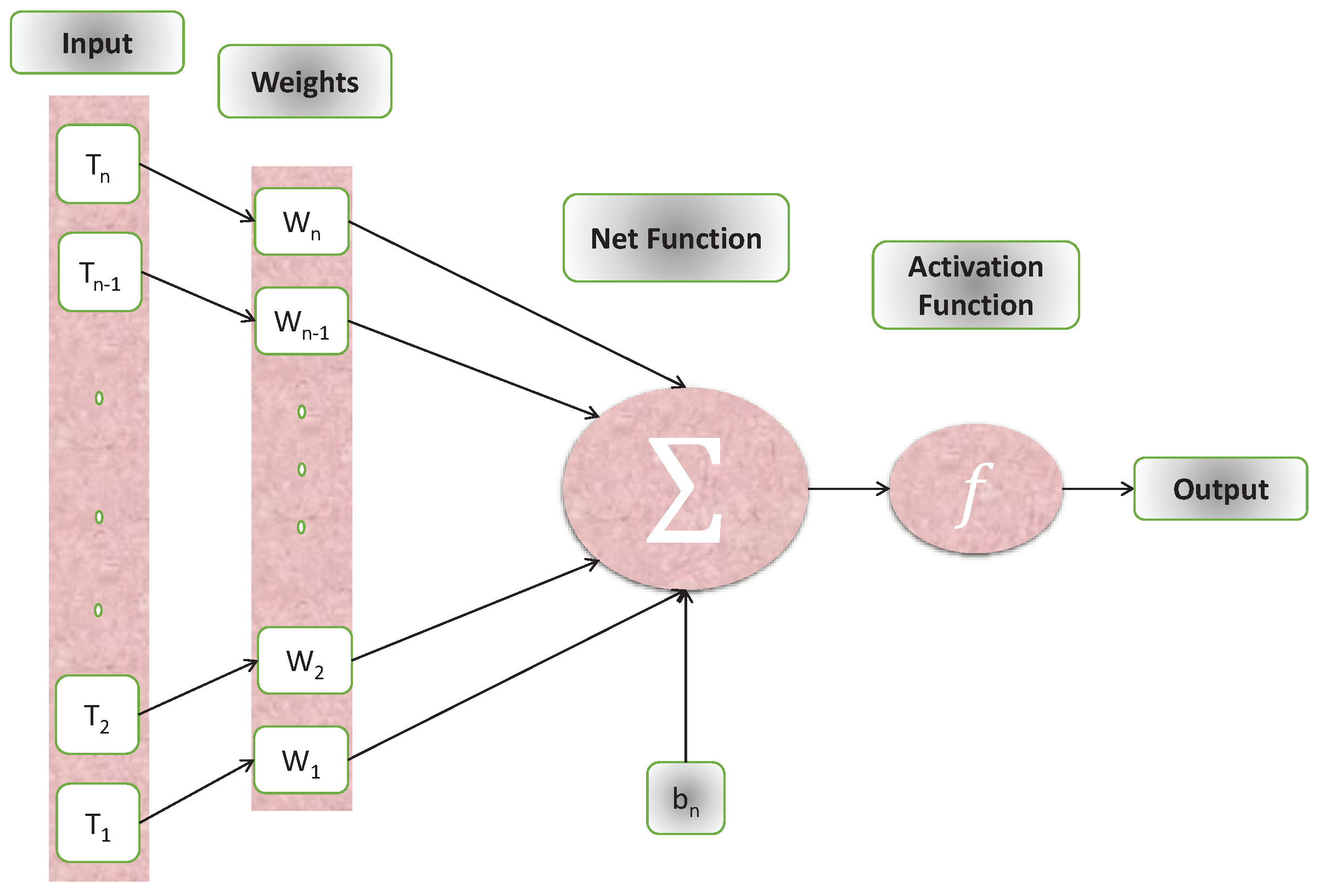
- For different cases of the problem, the Levenberg Marquardt method uses neural networks with 20 hidden neurons to approximate answers. Figure 1 depicts the NN’s-LMT approach as a single neuron model.
4. Results and Discussions
5. Conclusions
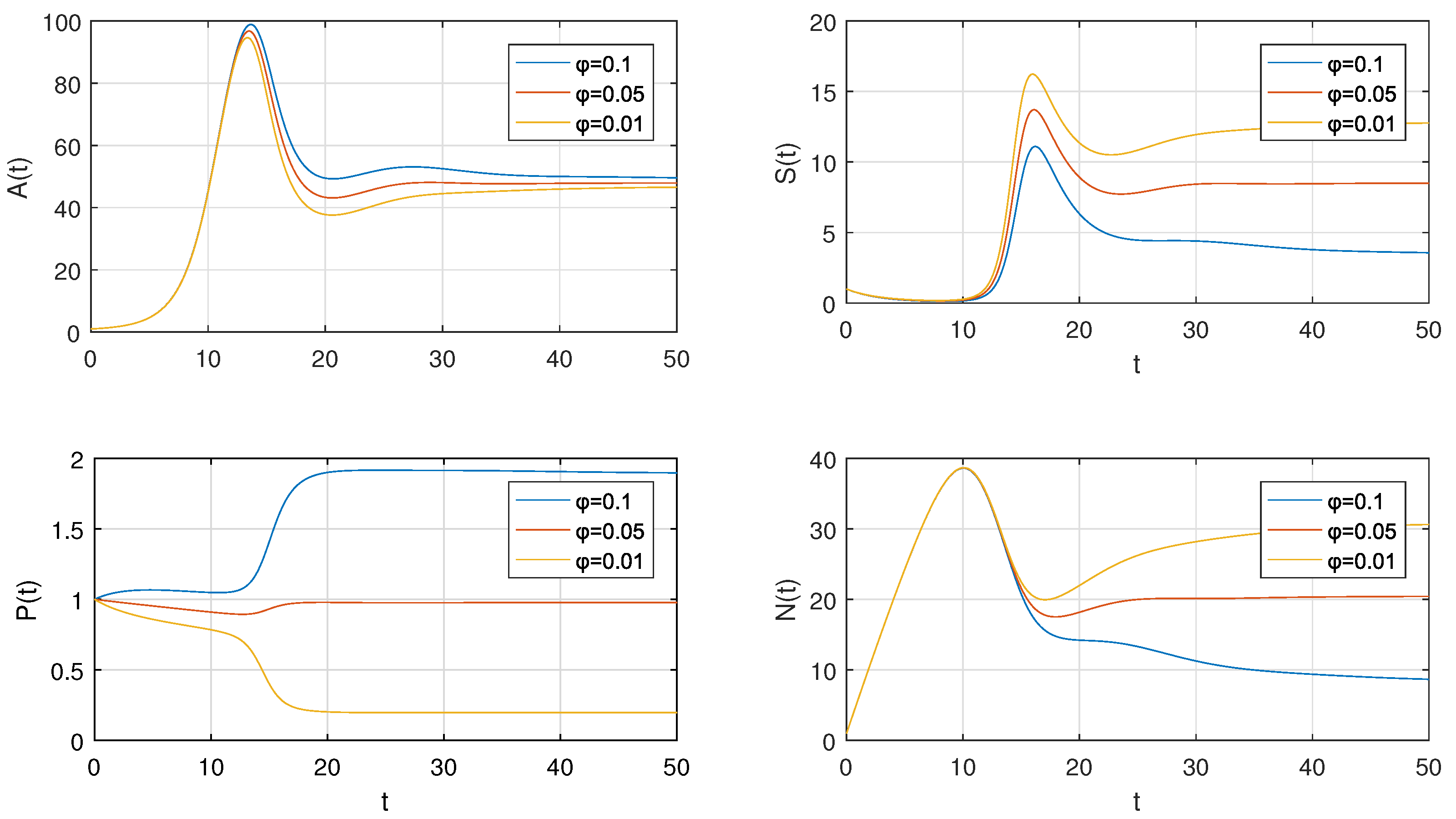
- Results shows in the figure illustrate that the decrease in spraying rate of insecticides causes decrease in crop production and insecticides concentration while increases the insects density and external effort.
- To relate the sparing rate of insecticides with the given model is that it relates inversely with crop production and insecticides concentration while directly relates to incests density and external efforts.
- Thorough graphical analysis is performed using mean squared error, error histograms, absolute errors, regressions, and computing complexity to demonstrate the resilience, correctness, and efficiency of the developed system.
Author Contributions
Funding
Institutional Review Board Statement
Informed Consent Statement
Data Availability Statement
Acknowledgments
Conflicts of Interest
References
- FSIN: Global Report on Food Crises. 2019. Available online: https://www.wfp.org/publications/2019-global-report-food-crises (accessed on 15 December 2021).
- Oerke, E.C. Crop losses to pests. J. Agric. Sci. 2006, 144, 31–43. [Google Scholar] [CrossRef]
- Shankar, C.; Dhyani, S.K. Insect pest of Jatropha curcas L. and the potential for their management. Curr. Sci. 2006, 91, 162–163. [Google Scholar]
- Sun, S.; Chen, L. Mathematical modelling to control a pest population by infected pests. Appl. Math. Model. 2009, 33, 2864–2873. [Google Scholar] [CrossRef]
- Xiao, Y.N.; Chen, L.S. Modeling and analysis of a predator-prey model with disease in the prey. Math. Biosci. 2001, 171, 59–82. [Google Scholar] [CrossRef]
- Wang, X.; Tao, Y.; Song, X. Analysis of pest-epidemic model by releasing diseased pest with impulsive transmission. Nonlinear Dyn. 2011, 65, 175–185. [Google Scholar] [CrossRef]
- Tang, S.; Cheke, R.A. State-dependent impulsive models of integrated pest management (IPM) strategies and their dynamic consequences. J. Math. Biol. 2005, 50, 257–292. [Google Scholar] [CrossRef] [PubMed]
- Misra, A.K.; Jha, N.; Patel, R. Modeling the Effects of Insects and Insecticides with External Efforts on Agricultural Crops. Differ. Equ. Dyn. Syst. 2020, 28, 1–18. [Google Scholar] [CrossRef]
- Uyovbisere, E.O.; Lombim, G. Efficient fertilizer use for increased crop production: The sub-humid Nigeria experience. Fertil. Res. 1991, 29, 81–94. [Google Scholar] [CrossRef]
- Misra, A.K.; Tiwari, P.K.; Chandra, P. Modeling the control of algal bloom in a lake by applying some external efforts with time delay. Differ. Equ. Dyn. Syst. 2017, 29, 539–568. [Google Scholar] [CrossRef]
- Lambert, J.D. Numerical Methods for Ordinary Differential Systems: The Initial Value Problem; John Wiley and Sons: Chichester, UK, 1991. [Google Scholar]
- Mickens, R.E. Nonstandard Finite Difference Models of Differential Equations; World Scientific: River Edge, NJ, USA, 1994. [Google Scholar]
- Mickens, R.E. Nonstandard finite difference schemes for differential equations. J. Differ. Equ. Appl. 2002, 8, 823–847. [Google Scholar] [CrossRef]
- Anguelov, R.; Lubuma, J.M.S. Contributions to the mathematics of the nonstandard finite difference method and applications. Numer. Methods Partial Differ. Equ. 2001, 17, 518–543. [Google Scholar] [CrossRef]
- Mickens, R.E. Dynamic consistency: A fundamental principle for constructing nonstandard finite difference schemes for differential equations. J. Differ. Equ. Appl. 2005, 11, 645–653. [Google Scholar] [CrossRef]
- Patidar, K.C. Nonstandard finite difference methods: Recent trends and further developments. J. Differ. Equ. Appl. 2016, 22, 817–849. [Google Scholar] [CrossRef]
- Obayomi, A.A.; Olabode, B.T. Comparative analysis of standard and non-standard finite difference schemes for the logistic equations. J. Emerg. Trends Eng. Appl. Sci. (JETEAS) 2013, 4, 317–321. [Google Scholar]
- Dimitrov, D.T.; Kojouharov, H.V. Positive and elementary stable nonstandard numerical methods with applications to predator-prey models. J. Comput. Appl. Math. 2006, 1–2, 98–108. [Google Scholar] [CrossRef]
- Chen-Charpentiera, B.M.; Dimitrovb, D.T.; Kojouharov, H.V. Combined nonstandard numerical methods for ODEs with polynomial right-hand sides. Math. Comput. Simul. 2006, 73, 105–113. [Google Scholar] [CrossRef]
- Anguelov, R.; Kama, P.; Lubuma, J.M.S. On non-standard finite difference models of reaction-diffusion equations. J. Comput. Appl. Math. 2005, 175, 11–29. [Google Scholar] [CrossRef][Green Version]
- Jansen, H.; Twizell, E.H. An unconditionally convergentdiscretization of the SEIR model. Math. Comput. Simul. 2002, 58, 147–158. [Google Scholar] [CrossRef]
- Basir, F.A.; Banerjee, A.; Ray, S. Role of farming awareness in crop pest management: A mathematical model. J. Theor. Biol. 2019, 461, 59–67. [Google Scholar] [CrossRef] [PubMed]
- Misra, A.K.; Jha, N.; Patel, R. Modeling the effects of insects and insecticides on agricultural crops with NSFD method. J. Appl. Math. Comput. 2020, 63, 197–215. [Google Scholar] [CrossRef]


| Parameter | Representation | Value | Source |
|---|---|---|---|
| r | Crop intrinsic growth rate | 0.2 | [22] |
| K | Carrying capacity of crop | 50 | [22] |
| Insect crop consumption rate | 0.025 | [22] | |
| Crop production rising as a result of external efforts | 0.01 | [23] | |
| Insect conversion efficiency | 0.6 | [23] | |
| Insect mortality owing to intra-specific competition | 0.05 | [22] | |
| Insecticide spray rate | 0.1 | [23] | |
| Insecticide depletion rate | 0.01 | [23] | |
| Insecticide uptake rate | 0.05 | [23] | |
| Insects depletion rate because of insecticides | 6 | [23] | |
| External effort application rate | 0.1 | [8] | |
| External efforts’ depletion rate | 0.01 | [8] |
| Index | Description |
|---|---|
| Training samples | |
| Validation samples | |
| Testing samples | |
| Hidden Neuron | 20 |
| Maximum Iteration | 1000 |
| Max. Validation fails | 6 |
| Learning methodology | Lavenberg-Marquardt |
| A(t) | S(t) | P(t) | N(t) | |
|---|---|---|---|---|
| Hidden Neuron | 20 | 20 | 20 | 20 |
| Training | ||||
| Validation | ||||
| Testing | ||||
| Gradient | ||||
| Mu | ||||
| Epochs | 1000 | 1000 | 480 | 1000 |
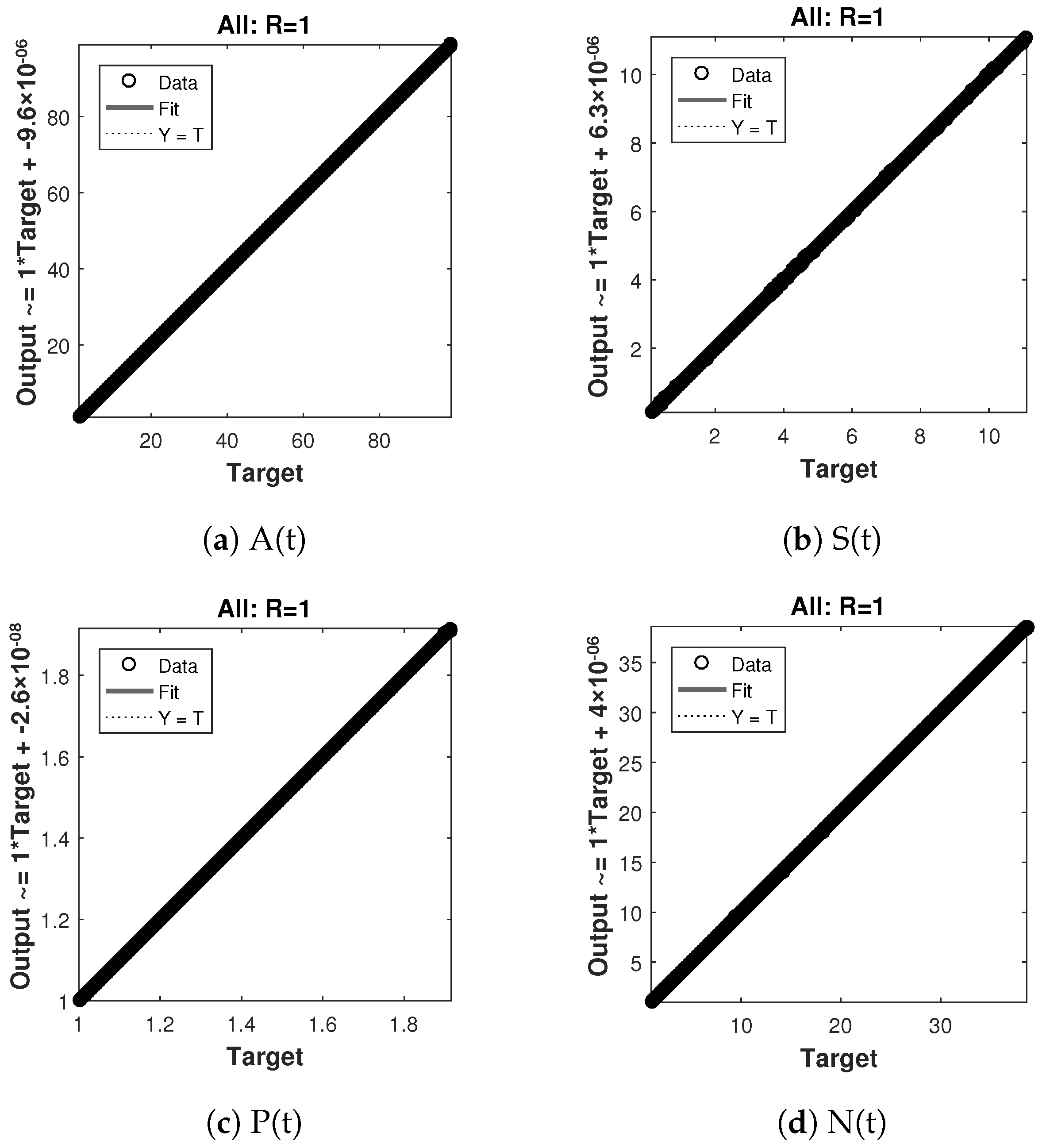
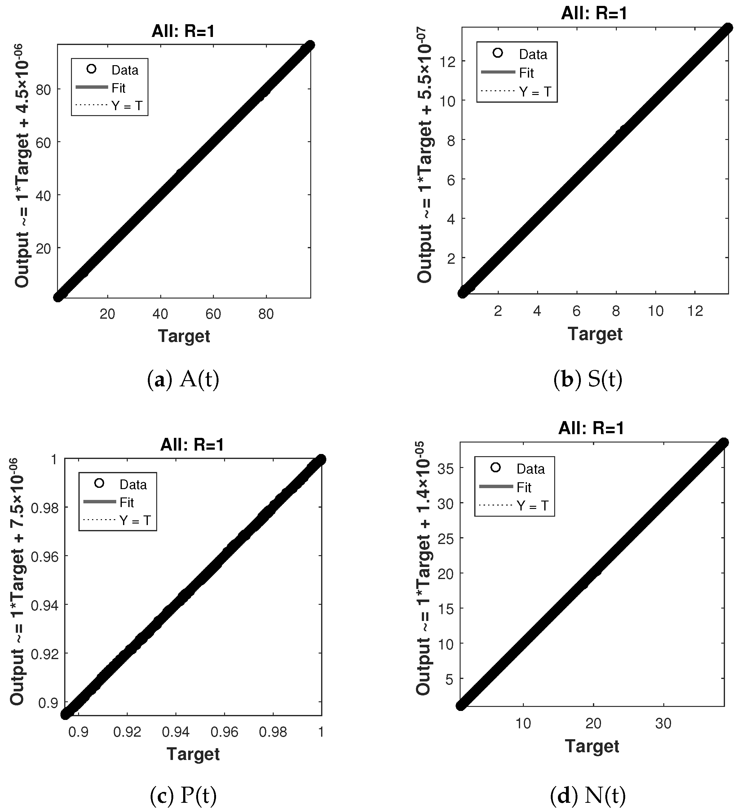
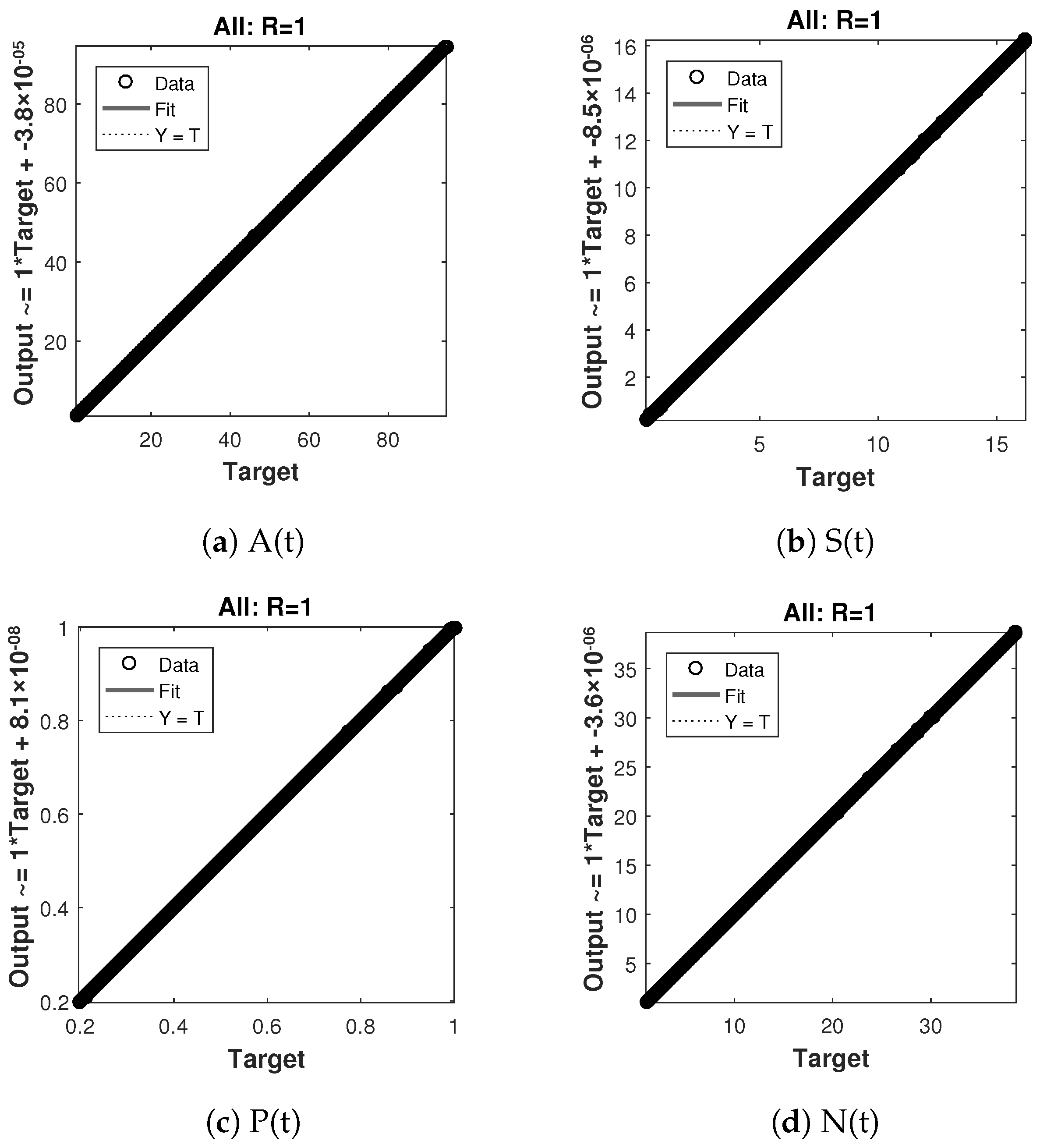
| Regression | 1 | 1 | 1 | 1 |
| Time | ≤10 s | ≤10 s | ≤10 s | ≤10 s |
| A(t) | S(t) | P(t) | N(t) | |
|---|---|---|---|---|
| Hidden Neuron | 20 | 20 | 20 | 20 |
| Training | ||||
| Validation | ||||
| Testing | ||||
| Gradient | ||||
| Mu | ||||
| Epochs | 1000 | 1000 | 27 | 1000 |
| Regression | 1 | 1 | 1 | 1 |
| Time | ≤10 s | ≤10 s | ≤10 s | ≤10 s |
| A(t) | S(t) | P(t) | N(t) | |
|---|---|---|---|---|
| Hidden Neuron | 20 | 20 | 20 | 20 |
| Training | ||||
| Validation | ||||
| Testing | ||||
| Gradient | ||||
| Mu | ||||
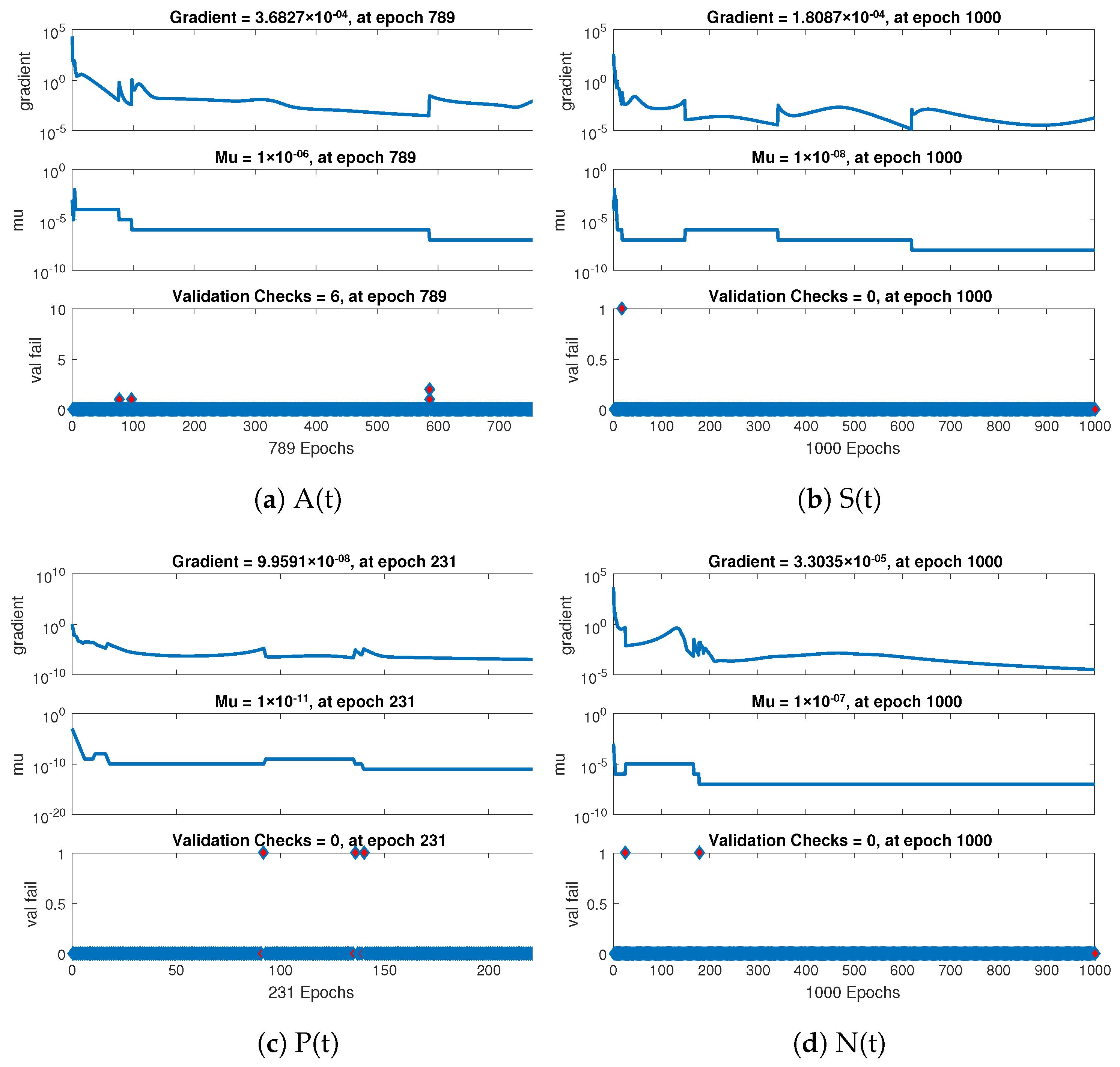
| Epochs | 789 | 1000 | 231 | 1000 |
| Regression | 1 | 1 | 1 | 1 |
| Time | ≤10 s | ≤10 s | ≤10 s | ≤10 s |
| Inputs | 1 | 2 | 3 | 4 | 5 | 6 | 7 | 8 | 9 | 10 |
|---|---|---|---|---|---|---|---|---|---|---|
| Numerical solutions | 1.231999 | 1.600315 | 2.184486 | 3.122899 | 4.656205 | 7.198827 | 11.43996 | 18.42872 | 29.45704 | 45.33719 |
| NN-LMA | 1.23214 | 1.600123 | 2.184666 | 3.122719 | 4.656247 | 7.198916 | 11.43973 | 18.4289 | 29.4569 | 45.33731 |
| Numerical solutions | 0.718154 | 0.520317 | 0.381155 | 0.283382 | 0.215257 | 0.168978 | 0.139796 | 0.125909 | 0.129818 | 0.163819 |
| NN-LMA | 0.717992 | 0.520488 | 0.38101 | 0.283403 | 0.21541 | 0.168843 | 0.139648 | 0.126113 | 0.130011 | 0.163525 |
| Numerical solutions | 1.031674 | 1.050653 | 1.061166 | 1.065945 | 1.066816 | 1.065051 | 1.061585 | 1.057178 | 1.052588 | 1.048885 |
| NN-LMA | 1.031675 | 1.050653 | 1.061167 | 1.065943 | 1.066818 | 1.065049 | 1.061586 | 1.05718 | 1.052586 | 1.048888 |
| Numerical solutions | 5.854973 | 10.63225 | 15.31545 | 19.87775 | 24.27422 | 28.42849 | 32.21092 | 35.40698 | 37.68503 | 38.60243 |
| NN-LMA | 5.855071 | 10.63231 | 15.31542 | 19.87763 | 24.27445 | 28.42841 | 32.21072 | 35.40719 | 37.68505 | 38.60219 |
| Inputs | 1 | 2 | 3 | 4 | 5 | 6 | 7 | 8 | 9 | 10 |
|---|---|---|---|---|---|---|---|---|---|---|
| Numerical solutions | 1.231945 | 1.599908 | 2.183103 | 3.119391 | 4.64842 | 7.182779 | 11.40845 | 18.36951 | 29.35154 | 45.16059 |
| NN-LMA | 1.232365 | 1.599246 | 2.183918 | 3.118602 | 4.649011 | 7.182732 | 11.40773 | 18.37041 | 29.35108 | 45.1601 |
| Numerical solutions | 0.722854 | 0.532449 | 0.399239 | 0.305263 | 0.239264 | 0.194265 | 0.166499 | 0.155516 | 0.16636 | 0.217773 |
| NN-LMA | 0.722864 | 0.532416 | 0.399263 | 0.305272 | 0.239222 | 0.194298 | 0.166512 | 0.155474 | 0.166413 | 0.217726 |
| Numerical solutions | 0.990247 | 0.980835 | 0.971617 | 0.962519 | 0.953504 | 0.94456 | 0.935694 | 0.926928 | 0.918317 | 0.909981 |
| NN-LMA | 0.990207 | 0.980864 | 0.971587 | 0.96255 | 0.953471 | 0.94458 | 0.935701 | 0.926895 | 0.918334 | 0.910002 |
| Numerical solutions | 5.854975 | 10.63227 | 15.31555 | 19.87808 | 24.27509 | 28.43049 | 32.21519 | 35.4156 | 37.70158 | 38.63262 |
| NN-LMA | 5.85497 | 10.63235 | 15.31552 | 19.87813 | 24.27513 | 28.43043 | 32.21524 | 35.41562 | 37.70151 | 38.63267 |
| Inputs | 1 | 2 | 3 | 4 | 5 | 6 | 7 | 8 | 9 | 10 |
|---|---|---|---|---|---|---|---|---|---|---|
| Numerical solutions | 1.231901 | 1.599577 | 2.181964 | 3.116445 | 4.641767 | 7.168801 | 11.38041 | 18.31555 | 29.2526 | 44.9884 |
| NN-LMA | 1.232696 | 1.598347 | 2.183202 | 3.115144 | 4.643025 | 7.167724 | 11.38085 | 18.31672 | 29.25189 | 44.99043 |
| Numerical solutions | 0.726644 | 0.542418 | 0.4145 | 0.324321 | 0.260921 | 0.217946 | 0.1925 | 0.185519 | 0.204918 | 0.277033 |
| NN-LMA | 0.726608 | 0.542258 | 0.414658 | 0.324249 | 0.260798 | 0.218211 | 0.192249 | 0.185623 | 0.20494 | 0.276839 |
| Numerical solutions | 0.956984 | 0.924296 | 0.898302 | 0.876817 | 0.858437 | 0.842199 | 0.827383 | 0.81337 | 0.799473 | 0.784613 |
| NN-LMA | 0.956987 | 0.924286 | 0.898311 | 0.876807 | 0.858447 | 0.842192 | 0.827382 | 0.813377 | 0.799465 | 0.784617 |
| Numerical solutions | 5.854976 | 10.63229 | 15.31563 | 19.87836 | 24.27582 | 28.4322 | 32.2189 | 35.42322 | 37.71655 | 38.66066 |
| NN-LMA | 5.855104 | 10.63241 | 15.3153 | 19.87845 | 24.27608 | 28.43191 | 32.21896 | 35.4234 | 37.71626 | 38.66098 |
Publisher’s Note: MDPI stays neutral with regard to jurisdictional claims in published maps and institutional affiliations. |
© 2022 by the authors. Licensee MDPI, Basel, Switzerland. This article is an open access article distributed under the terms and conditions of the Creative Commons Attribution (CC BY) license (https://creativecommons.org/licenses/by/4.0/).
Share and Cite
Sulaiman, M.; Umar, M.; Nonlaopon, K.; Alshammari, F.S. The Quantitative Features Analysis of the Nonlinear Model of Crop Production by Hybrid Soft Computing Paradigm. Agronomy 2022, 12, 799. https://doi.org/10.3390/agronomy12040799
Sulaiman M, Umar M, Nonlaopon K, Alshammari FS. The Quantitative Features Analysis of the Nonlinear Model of Crop Production by Hybrid Soft Computing Paradigm. Agronomy. 2022; 12(4):799. https://doi.org/10.3390/agronomy12040799
Chicago/Turabian StyleSulaiman, Muhammad, Muhammad Umar, Kamsing Nonlaopon, and Fahad Sameer Alshammari. 2022. "The Quantitative Features Analysis of the Nonlinear Model of Crop Production by Hybrid Soft Computing Paradigm" Agronomy 12, no. 4: 799. https://doi.org/10.3390/agronomy12040799
APA StyleSulaiman, M., Umar, M., Nonlaopon, K., & Alshammari, F. S. (2022). The Quantitative Features Analysis of the Nonlinear Model of Crop Production by Hybrid Soft Computing Paradigm. Agronomy, 12(4), 799. https://doi.org/10.3390/agronomy12040799