AgroML: An Open-Source Repository to Forecast Reference Evapotranspiration in Different Geo-Climatic Conditions Using Machine Learning and Transformer-Based Models

Abstract

Accurately forecasting reference evapotranspiration (ET₀) values is crucial to improve crop irrigation scheduling, allowing anticipated planning decisions and optimized water resource management and agricultural production. In this work, a recent state-of-the-art architecture has been adapted and deployed for multivariate input time series forecasting (transformers) using past values of ET₀ and temperature-based parameters (28 input configurations) to forecast daily ET₀ up to a week (1 to 7 days). Additionally, it has been compared to standard machine learning models such as multilayer perceptron (MLP), random forest (RF), support vector machine (SVM), extreme learning machine (ELM), convolutional neural network (CNN), long short-term memory (LSTM), and two baselines (historical monthly mean value and a moving average of the previous seven days) in five locations with different geo-climatic characteristics in the Andalusian region, Southern Spain. In general, machine learning models significantly outperformed the baselines. Furthermore, the accuracy dramatically dropped when forecasting ET₀ for any horizon longer than three days. SVM, ELM, and RF using configurations I, III, IV, and IX outperformed, on average, the rest of the configurations in most cases. The best NSE values ranged from 0.934 in Córdoba to 0.869 in Tabernas, using SVM. The best RMSE, on average, ranged from 0.704 mm/day for Málaga to 0.883 mm/day for Conil using RF. In terms of MBE, most models and cases performed very accurately, with a total average performance of 0.011 mm/day. We found a relationship in performance regarding the aridity index and the distance to the sea. The higher the aridity index at inland locations, the better results were obtained in forecasts. On the other hand, for coastal sites, the higher the aridity index, the higher the error. Due to the good performance and the availability as an open-source repository of these models, they can be used to accurately forecast ET₀ in different geo-climatic conditions, helping to increase efficiency in tasks of great agronomic importance, especially in areas with low rainfall or where water resources are limiting for the development of crops.

1. Introduction

The worldwide population is increasing to alarming values that will require almost 50% more food to meet the demand in 2050 [1]. Therefore, research into new methodologies to outperform agroclimatic forecasts (solar radiation, precipitation, or evapotranspiration) is a relevant task that allows the optimization of water resource management, the improvement of irrigation scheduling, and, indeed, contributes to the great challenge of increasing food production. Furthermore, it is significantly impactful in arid and semiarid areas such as the Andalusian region (Southern Spain), where crop water uses are elevated and the scarce precipitation is limiting growth and agricultural yield.

Crop evapotranspiration measures the crops’ water demand, being affected by atmospheric parameters (such as temperature, wind speed, or solar radiation), specific crop type, soil characteristics, as well as management and environmental conditions. The evapotranspiration rate from a reference surface with no shortage of water is named reference evapotranspiration (ET₀), which studies the evaporative demand of the atmosphere independently of the surface, the crop type, its development stage, and the management practices. Its calculation can be accurately determined using physics-based methods such as the FAO56-PM [2], which has been assessed globally in different climatic conditions and countries, including Korea [3], Argentina [4], and Tunisia [5], among others. However, measuring all the required parameters (air temperature, relative humidity, wind speed, and solar radiation) is very costly in installation and maintenance. Moreover, Automated Weather Stations (AWS) usually contain non-reliable long-term datasets, mainly for wind speed and solar radiation, due to a lack of maintenance or miscalibration [6]. These are the reasons why the geographical density of complete AWS is generally low, especially in rural areas and developing countries [7,8].

Therefore, developing new algorithms with fewer climatic input parameters is of high interest. In this context, Hargreaves and Samani [9] introduced an empirical equation (HS) that uses maximum and minimum daily air temperature values (Tx and Tn, respectively) and extraterrestrial solar radiation (Ra). Different studies have assessed HS in different aridity conditions and countries, such as Iran [10], Italy [11], Bolivia [11], China [12], and others. Nevertheless, advances in computation during the last several decades led to the application of new methodologies based on Artificial Intelligence (AI) with a very intensive computational cost. Thanks to the progress in CPU and GPU computation, the time spent training these models has dropped significantly, allowing scientists to apply them without needing a vast CPU/GPU farm and obtaining promising results in all sectors, especially agriculture. For example, Karimi et al. [13] evaluated the performance of random forest (RF) and other empirical methods to estimate ET₀ when several meteorological data were missing. RF surpassed the other models for temperature-based data availability when using Tx, Tn, Ra, and relative humidity (RH) as input features. Ferreira and da Cunha [14] assessed RF, extreme gradient boosting (XGB), multilayer perceptron (MLP), and convolutional neural network (CNN) to estimate daily ET₀ through different approaches, using hourly temperature and relative humidity as features in different AWS in Brazil. CNN outperformed the rest of the models for most statistics and locations in both local and regional approaches. However, no optimization algorithm was used during hyperparameter tuning. Yan et al. [15] evaluated XGB to estimate daily ET₀ in two different regions (an arid and humid region) from China and seven meteorological input combinations using maximum and minimum daily temperature (Tx and Tn, respectively), extraterrestrial solar radiation (Ra), relative humidity (RH), wind speed (U₂), and sunshine hours (n). In order to tune the different hyperparameters, the Whale Optimization Algorithm (WOA) was used. Their results showed that using local and external (neighbor stations) datasets obtained even better performance than using only local data in some cases. Therefore, this strategy is very promising when there is a lack of long-term records. Wu et al. [16] studied the performance of extreme learning machines (ELM) in different locations from China. They analyzed the use of the K-means clustering algorithm and the Firefly Algorithm (FFA) to estimate monthly mean daily ET₀ using Tx, Tn, Ra, and Tm (mean daily temperature). Nourani et al. [17] assessed support vector regression (SVR), Adaptive Fuzzy Inference System (ANFIS), MLP, and multiple linear regression (MLR) to forecast monthly ET₀ in Turkey, North Cyprus, and Iraq. Moreover, three ensemble methods were applied (simple averaging, weighted averaging, and neural ensemble) to outperform the performance and reliability of single modeling. The use of neural ensemble models highly outperformed single modeling in all cases, although simple and weighted averaging did not significantly perform better. Ferreira and da Cunha [18] evaluated the performance of daily ET₀ forecasts (up to 7 days) using CNN, long short-term memory (LSTM), CNN-LSTM, RF, and MLP using hourly data from different weather stations with heterogeneous aridity index characteristics in Brazil. In all cases, the use of the machine learning (ML) models outperformed the baselines, where CNN-LSTM performed the best in both local and regional scenarios using Tx, Tn, maximum and minimum relative humidity (RHx and RHn, respectively), wind speed, solar radiation (Rs), Ra, the day of the year (DOY), and ET₀ values from a lag window in the past (up to 30 days). In order to tune the different hyperparameters, a random search algorithm with 30 epochs was used.

In addition to these well-known and standard ML models, new architectures have been recently developed to deal with natural language programming (NLP) problems with outstanding results, called transformers [19]. The transformer model is an encoder–decoder architecture based on a self-attention mechanism that looks at an input sequence and decides which timesteps are valuable. The promising results of transformers have fostered their use on time series problems due to its apparent relationship. In both types of problems, words/parameter values are more or less meaningful based on their position. Therefore, several scientists have evaluated attention-based architectures in forecasting problems. For example, Wu et al. [20] proposed an Adversarial Sparse Transformer (AST) based on generative adversarial networks (GAN). They assessed it to forecast five different public datasets: (I) an hourly time series electricity consumption dataset, (II) an hourly traffic level from the San Francisco dataset, (III) an hourly solar power production dataset, and (IV) an hourly time series dataset from the M4 competition. Furthermore, [21] analyzed a transformed-based architecture to forecast influenza-like illness (ILI), obtaining promising results. Finally, Li et al. [22] evaluated the performance of transformers in time series forecasting using the same public datasets as Wu et al. [20] and obtained more accurate modeling with long-term dependencies.

This work is motivated by the need to minimize error in daily ET₀ forecasts, which is one of the main drawbacks in the reviewed literature, as well as the outstanding and promising performance of transformers and transformer-based models in different fields. Thereby, this work is the first one using a multivariate input transformer-based architecture in order to forecast daily ET₀ (from one to seven days ahead). The development and assessment have been carried out using past values of ET₀ and temperature-based measured variables as features in five sites of Andalusia (Córdoba, Málaga, Conil, Tabernas, and Aroche) with different geo-climatic characteristics. Moreover, standard ML models such as RF, MLP, SVR, ELM, CNN, and LSTM have been also evaluated in conjunction with Bayesian optimization to tune all their different hyperparameters. Thus, the main objectives of this work are (a) to assess the performance of the proposed transformer model to forecast ET₀ and to compare it to standard ML models and two simple baselines (historical monthly mean value and mean of previous seven days); (b) to evaluate different input feature configurations based on ET₀ past values and several temperature-based features to forecast ET₀, and (c) to analyze the forecast efficiency depending on the different geo-climatic characteristics of the sites.

2. Materials and Methods

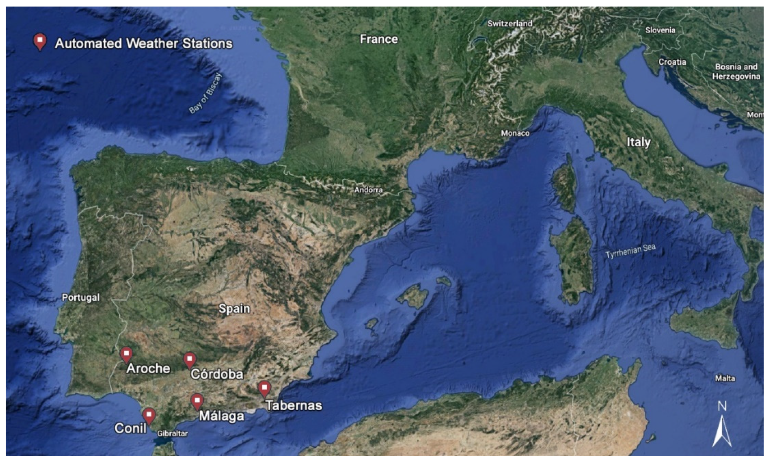
2.1. Study Area and Dataset

Andalusia is located in the southwest of Europe, ranging from 37° to 39° N, from 1° to 7° W, and occupying an extension of 87,268 km². This work was carried out with data from five locations in Andalusia (Figure 1), with different geo-climatic characteristics and representing great variability in terms of UNEP aridity index [23] in this region (ranging from 0.555—dry subhumid—in Aroche, to 0.177—arid—in Tabernas). The coordinates and other characteristics of the AWS are reported in

Table 1. Geo-climatic characteristics of the locations assessed in this work (ARO—Aroche, CON—Conil de la Frontera, COR—Córdoba, MAG—Málaga, and TAB—Tabernas). Time period from 2000 to 2018.

Site	Lon. (° W)	Lat. (° N)	Alt. (m)	Mean Annual Precipitation (mm)	UNEP Aridity Index	Total Available Days
Aroche (ARO)	6.94	37.95	293	632	0.555 (dry-subhumid)	6399
Conil de la Frontera (CON)	6.13	36.33	22	470	0.479 (semiarid)	5868
Córdoba (COR)	4.80	37.85	94	589	0.462 (semiarid)	6397
Málaga (MAG)	4.53	36.75	55	434	0.366 (semiarid)	6438
Tabernas (TAB)	2.30	37.09	502	237	0.178 (arid)	6694

. In contrast, in

Table 2. Minimum (Min), mean, maximum (Max), and standard deviation (Std) values of all the daily parameters measured: maximum air temperature (Tx), mean air temperature (Tm), minimum air temperature (Tn), maximum relative humidity (RHx), mean relative humidity (RHm), minimum relative humidity (RHn), wind speed at 2 m height (U₂), solar radiation (Rs), reference evapotranspiration (ET₀) at each location (ARO—Aroche, CON—Conil de la Frontera, COR—Córdoba, MAG—Málaga, and TAB—Tabernas) and for the whole dataset (2000–2018).

		Tx (°C)	Tm (°C)	Tn (°C)	RHx (%)	RHm (%)	RHn (%)	U2 (m/s)	Rs (MJ/m2 day)	ET0 (mm)
ARO	Min	2.5	−0.2	−8.0	32.5	17.2	5.0	0.3	1.0	0.3
	Mean	23.2	16.1	8.9	89.5	65.9	39.0	1.2	17.8	3.2
	Max	44.0	34.1	24.9	100.0	100.0	100.0	5.8	34.3	8.7
	Std	8.1	6.8	5.6	11.2	17.7	19.4	0.5	8.8	2.0
CON	Min	6.4	0.7	−5.3	39.9	24.3	6.9	0.0	0.5	0.4
	Mean	23.0	17.4	12.1	89.3	72.5	50.5	1.3	18.0	3.2
	Max	41.3	31.9	26.9	100.0	99.6	97.1	7.9	31.7	9.3
	Std	5.7	5.2	5.3	9.0	12.3	14.6	1.0	7.8	1.8
COR	Min	3.3	0.0	−8.3	38.9	21.8	4.3	0.0	0.5	0.3
	Mean	24.6	17.4	11.0	86.8	64.1	37.3	1.6	17.7	3.6
	Max	45.7	34.7	27.6	100.0	100.0	100.0	7.5	33.2	9.6
	Std	8.5	7.3	6.2	12.0	18.1	19.3	0.7	8.5	2.3
MAG	Min	6.2	3.3	−4.2	36.0	19.4	4.6	0.0	0.3	0.4
	Mean	23.9	18.2	12.6	85.1	63.4	39.1	1.3	18.2	3.4
	Max	42.7	33.7	26.8	100.0	99.7	98.3	4.6	32.4	10.3
	Std	6.3	5.8	5.5	10.5	14.2	15.1	0.5	8.2	1.9
TAB	Min	4.3	−1.2	−8.2	28.6	16.8	2.8	0.1	0.2	0.4
	Mean	23.2	16.4	9.8	85.7	59.9	32.9	1.9	18.4	3.8
	Max	42.5	32.1	26.0	100.0	97.5	95.0	9.9	32.8	10.6
	Std	7.2	6.6	6.2	11.9	15.1	14.8	0.9	7.8	2.0

, the minimum, mean, maximum, and standard deviation values of minimum, mean, and maximum daily air temperature (Tn, Tm, and Tx, respectively), relative humidity (RHn, RHm, RHx, respectively), wind speed (U₂), solar radiation (Rs), and reference evapotranspiration (ET₀) data are shown. The dataset used in this study belongs to the Agroclimatic Information Network of Andalusia (RIA), which can be downloaded at https://www.juntadeandalucia.es/agriculturaypesca/ifapa/ria/servlet/FrontController (accessed on 1 February 2022).

In this work, because the accurate estimation of ET₀ using limited meteorological data has been improved in recent years [14,24] and due to the high availability of temperature records, only temperature-based and ET₀ values from the past have been used as input features to forecast ET₀. Specifically, two different windows have been evaluated, the use of 15 and 30 days from the past. Moreover, several temperature-based variables have been calculated, such as EnergyT (the area below the intraday temperature in a whole day), HourminTx (the time when Tx occurs), HourminTn (the time when Tn occurs), HourminSunset (the time when sunset occurs), HourminSunrise (the time when sunrise occurs), es (mean saturation vapor pressure), ea (actual vapor pressure) and VPD (vapor pressure deficit), Tx-Tn, HourminSunset-HourminTx, and HourminSunrise-HourminTn. All the configurations assessed in this work contained Tx, Tn, Tx-Tn, and Ra as features due to their very high Pearson correlation (Figure 2), and the rest of the configurations were selected based on their Pearson correlation values and the previous results on these same locations regarding ET₀ and solar radiation [24,25,26] estimations. The 27 different assessed configurations are shown in

Table 3. Configuration table with all configurations. HTx represents HourminTx, HTn represents HourminTn, HSs represents HourminSunset, and HSr represents HourminSunrise.

Conf.	Tx	Tn	Tx-Tn	Ra	EnergyT	ea	es	VPD	HTx	HTn	HSs-HTx	HSr-HTn	ET0
I	X	X	X	X		X							X
II	X	X	X	X	X	X							X
III	X	X	X	X	X		X						X
IV	X	X	X	X	X								X
V	X	X	X	X	X						X		X
VI	X	X	X	X	X							X	X
VII	X	X	X	X	X					X			X
VIII	X	X	X	X	X	X			X				X
IX	X	X	X	X	X		X		X				X
X	X	X	X	X	X				X				X
XI	X	X	X	X	X				X		X		X
XII	X	X	X	X	X				X			X	X
XIII	X	X	X	X	X	X	X	X	X	X	X	X	X
XIV	X	X	X	X	X	X			X	X			X
XV	X	X	X	X	X		X		X	X			X
XVI	X	X	X	X	X				X	X			X
XVII	X	X	X	X	X				X	X	X		X
XVIII	X	X	X	X	X				X	X		X	X
XIX	X	X	X	X	X			X	X	X			X
XX	X	X	X	X	X			X	X				X
XXI	X	X	X	X	X			X					X
XXII	X	X	X	X			X						X
XXIII	X	X	X	X									X
XXIV	X	X	X	X							X		X
XXV	X	X	X	X								X	X
XXVI	X	X	X	X						X			X
XXVII	X	X	X	X					X				X

.

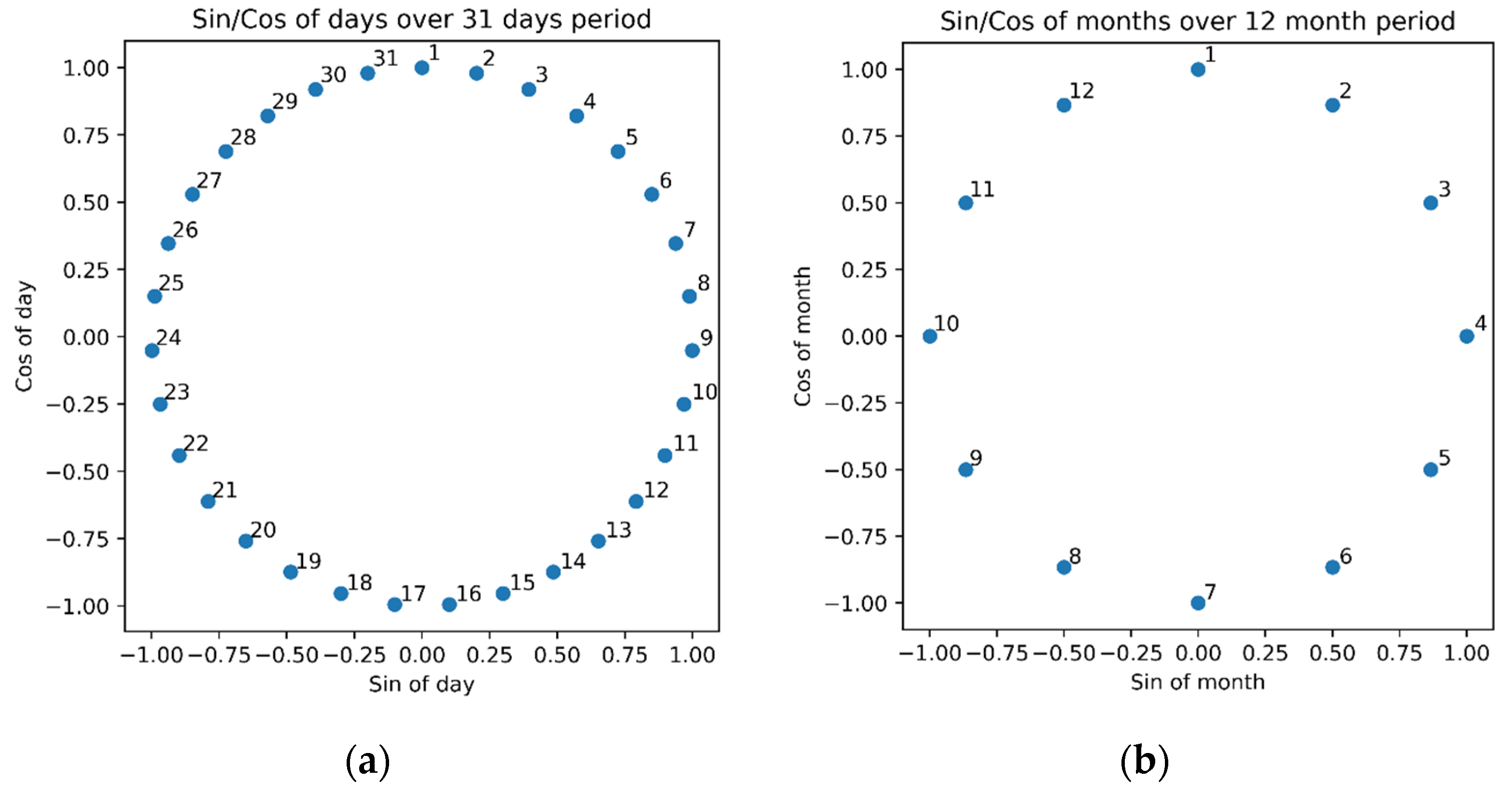
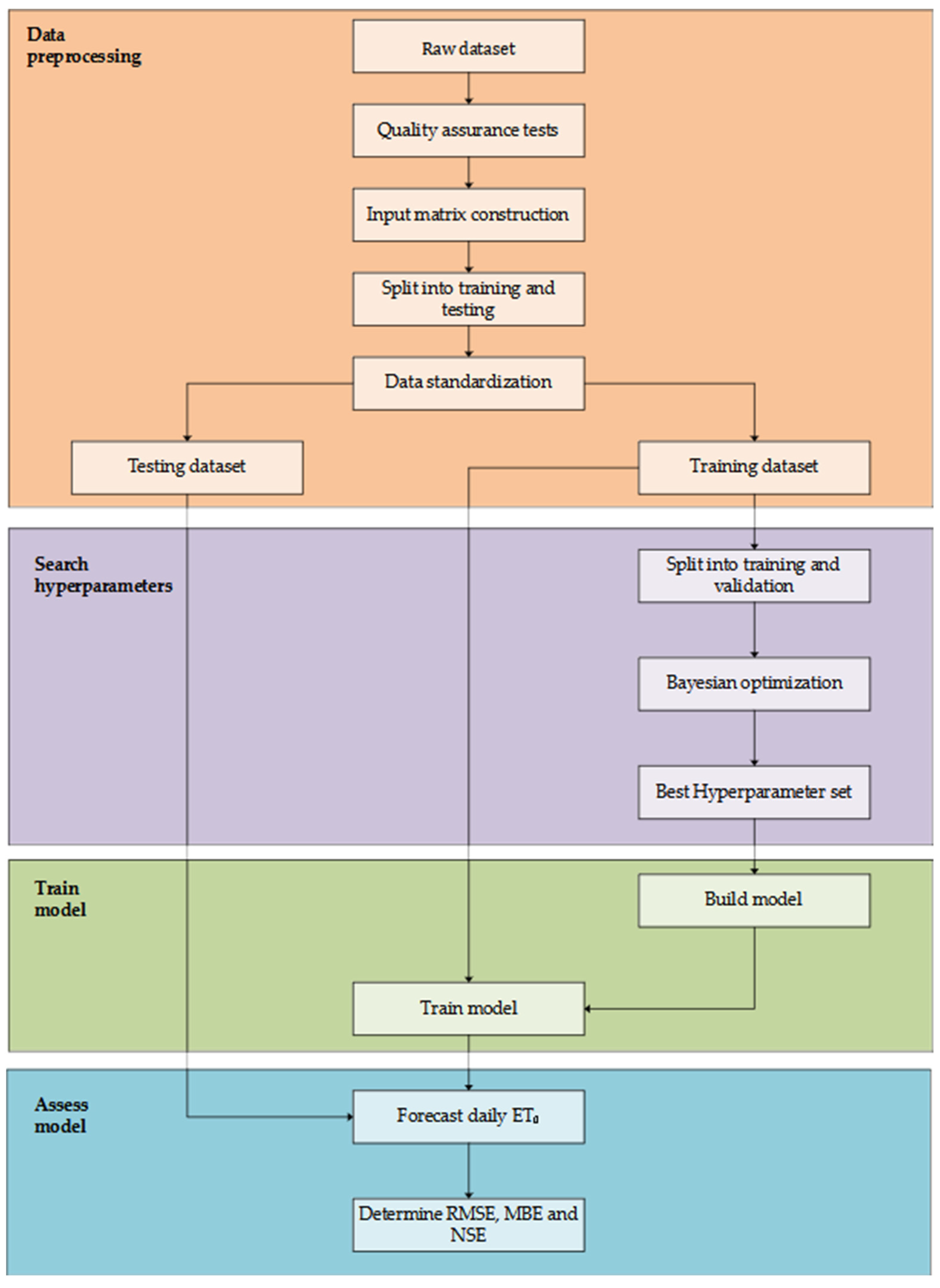
2.2. Preprocessing Methodology

In machine learning applications, a vital prerequisite to guarantee accurate modeling is the use of reliable datasets. In this work, the control guidelines reported by Estévez et al. [6] have been followed to identify erroneous and questionable data from sensor measurements by applying different tests (range, internal consistency, step, and persistence) and a spatial consistency test [27]. These quality assurance procedures have been successfully employed in different countries [4,28,29]. Afterward, the input and output matrices had to be built depending on the number of lag days from the past (15 or 30), the features to use (up to 27 input configurations), and the number of days to forecast (up to 7 days). In Figure 3 and Figure 4, a mind map with all the possibilities is shown. It is worth noting that a MIMO (Multiple Input Multiple Output) approach was used in models that allowed it, whereas a direct approach was considered in the others according to the results of Ferreira and da Cunha [18].

Consequently, using configuration 1 and 15 lag days as an example, the values from day to day—14 of Tx, Tn, Tx-Tn, Ra, ea, and ET₀ are used as input features (a total of 90 values) for all the ML models (except for transformers—see Section 2.5.7), where Tx and Tn are directly given by AWS, and Ra and ea can be calculated using Tx, Tn, and the latitude, as stated by [2]. Finally, ET₀ is calculated using the well-known FAO56-PM method.

Later, in order to train, tune all the hyperparameters, and assess the final performance of the model, for each location, the dataset was split into training (70% of the entire dataset length), validation (20% of the training dataset length), and testing (30% of the entire dataset length) using a holdout technique. Next, the Bayesian optimization algorithm was used to tune all the hyperparameters (the hyperparameter space can be seen in Table S1, Supplementary Materials). Eventually, after the best hyperparameter set was found, the final model was trained using the entire training dataset (70% of the entire dataset length) and evaluated using the testing dataset. Figure 5 shows an overview of this methodology.

2.3. Reference Evapotranspiration Calculation

In this work, the ET₀ (FAO56-PM) values were used as input and target values. They were determined following the procedure of [2], and can be mathematically expressed as Equation (1):

$${\mathrm{ET}}_0=\frac{0.408∆\left(\mathrm{Rn}-\mathrm{G}\right)+\gamma \frac{900}{T+273}{U}_2\left(\mathrm{es}-\mathrm{ea}\right)}{∆+\gamma \left(1+0.34{\mathrm{U}}_2\right)}$$

(1)

where ET₀ is the reference evapotranspiration (mm day⁻¹), 0.408 corresponds to a coefficient (MJ⁻¹ m² mm), $∆$ is the slope of the saturation vapor pressure versus temperature curve (kPa °C⁻¹), Rn is the net radiation calculated at the crop surface (MJ m⁻² day⁻¹), G is the soil heat flux density at the soil surface (MJ m⁻² day⁻¹), $\gamma$ is the psychrometric constant (kPa °C⁻¹), T is the mean daily air temperature (°C), U₂ is the mean daily wind speed at 2 m height (m s⁻¹), and es and ea are the saturation vapor pressure and the mean actual vapor pressure, respectively (kPa).

2.4. Baselines

In order to compare the performance of the developed models and configurations, it is crucial to have a baseline performance as a starting point. In this sense, two empirical baselines have been proposed in this work, following the methodology proposed by Ferreira and da Cunha [18]. In the first place, a moving average from the last 7 days was used. Secondly, the historical average monthly values from the training dataset were used for the corresponding forecast day.

2.5. Machine Learning Models

2.5.1. Multilayer Perceptron

The multilayer perceptron (MLP) is one of the most used agronomical and hydrological AI models [14,30,31]. Its popularity is based on its similarities to neurons in the biological nervous system, easy coding, and promising results in most cases. They are structured in three kinds of layers, the input and output layer, representing the inputs and outputs of the model, respectively, and the hidden layers, where all the neurons are located. The neurons work together to create stimuli (reference evapotranspiration forecast values) based on different inputs (the input matrix containing features from the past). A back-propagation algorithm makes the neurons learn (automatically update all weights and biases) and improve every mini batch every epoch. A single neuron architecture can be seen in Figure 6.

2.5.2. Extreme Learning Machine

Extreme learning machine models (ELM) were first introduced by Huang et al. [32] as a single hidden layer feed-forward neural network with the following main characteristics: (I) the input weights and biases are randomly generated and (II) the output weights and biases are analytically determined. As a result, these models do not require any training process and have a meager computational cost, with promising results in ET₀ [24,33,34]. However, on the other hand, when the model is working with massive datasets, the amount of random access memory (RAM) required is enormous.

2.5.3. Support Vector Machine for Regression

Support vector machine (SVM) models for regression tasks, also known as support vector regression (SVR) models, are supervised AI models based on a different functionality than neuron-based architectures such as MLP and ELM. They search for the best hyperplane (and its margins) that contains all data points. Thus, it could be easily related to linear regression with the flexibility of defining how much error can be considered acceptable. Moreover, one of their most important features is the use of kernels to allow the model to operate on a high-dimensional feature space. SVMs can be mathematically expressed as a minimization problem of Equation (2) with the constraints in Equation (3).

$$MIN \left(\frac{1}{2} \Vert {w\Vert }^2+C {\displaystyle \sum }_{i=1}^n\left|{\xi }_i\right| \right) \ge 0$$

(2)

$$\left|y_i-w_i{x}_i\right|\le \epsilon +\left|{\xi }_i\right|$$

(3)

where w_i corresponds to the weight vector, x_i to the input vector, y_i to the output vector, $\epsilon$ represents the margins, ξ represents the deviation of values to the margins, C is a coefficient to penalize deviation to the margins, and n is the length of the training dataset. For further details, the work of [35] can be consulted.

2.5.4. Random Forest

A random forest (RF) is composed of the conjunction of multiple tree-based models in order to improve the overall result (ensemble model). The general idea is that different models are trained on different data samples (bootstrap) and feature sets. Instead of searching for the best features when splitting nodes, it searches among a random subset of the features. Thus, it results in greater diversity and better final performance.

2.5.5. Convolutional Neural Network

Convolutional neural network (CNN) models were first developed for image classification problems, where the convolution algorithm captures local patterns to learn a representation of figures to classify them. Moreover, this process can be extrapolated to 1D sequences of data such as time series datasets. One of the advantages of using convolutions is that they can obtain local features’ relationships without the requirement of an extensive preprocessing method and can obtain outstanding results in ET₀ [14,36,37] and in other agro-climatic parameters [25,38,39].

Typically, such CNNs are composed of three layers: the convolutional layer, the pooling layer, and a fully connected layer. The convolutional layer is used to extract local relationships between the different features and timesteps. The pooling layer is added after the convolutional layer, and it gradually reduces the feature map. Finally, a fully connected layer is used to forecast the seven-day horizon ET₀ values (in this work). For further details, the work of Aloysius et al. [40] can be reviewed.

2.5.6. Long Short-Term Memory

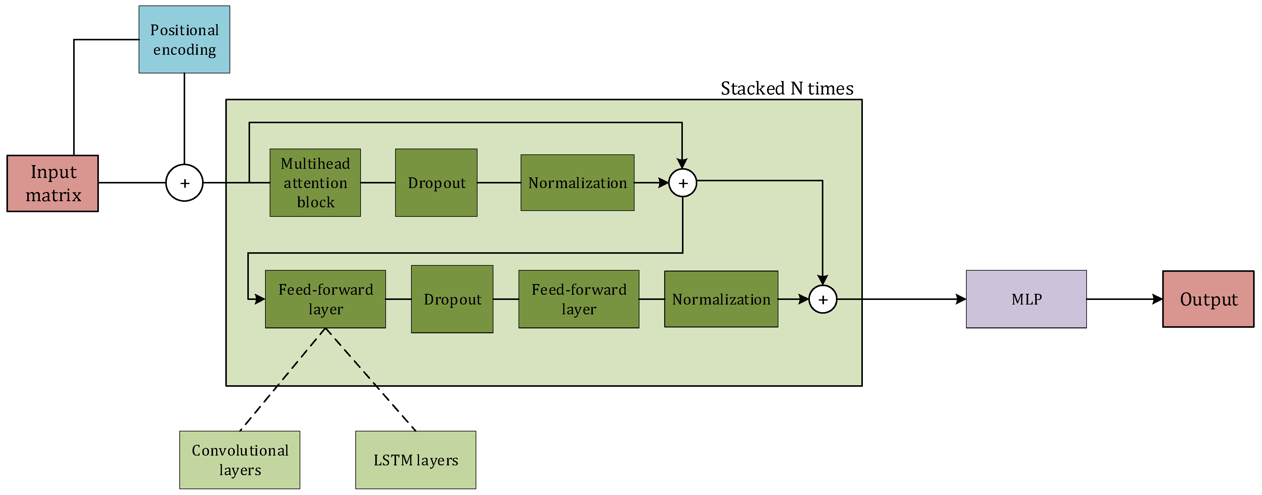
Long short-term memory (LSTM) models were first introduced by Hochreiter et al. [41] as a recurrent neural network (RNN)-based model that could deal with long-term dependencies and address the vanishing gradient problem. In order to control the information flow, the LSTM block contains an input gate, an output gate, a forget gate, a cell state, and a hidden state. The gates are in charge of deciding which information is allowed on the cell state, i.e., whether a piece of information is relevant to keep or forget during training. The cell and hidden state can be seen as the memory of the network, used to carry relevant information throughout the sequence.

2.5.7. Transformers

A new state-of-the-art architecture has been recently presented for NLP problems, the transformers [19]; see Figure 7. One of the main motivations of transformers is to deal with the vanishing gradient problem of LSTM when working with long sequences. Although LSTMs can theoretically propagate crucial information over infinitely long sequences, due to the vanishing gradient problem, they pay more attention to recent tokens and eventually forget earlier tokens. In contrast, transformers use an attention mechanism, which learns the relevant subset of the sequences to accomplish the specific task. For a single head, the operation can be expressed as Equation (4),

$$Attention\left(Q, K, V\right)=Softmax(\frac{Q K^T}{\sqrt{d_k}})V$$

(4)

where Q, K, and V represent the query, key, and value, respectively, as an analogy to a database, and d_k corresponds to queries and keys’ dimension. As stated by Yıldırım and Asgari-Chenaghlu (2021), the attention mechanism can be defined as follows: “This can also be seen as a database where we use the query and keys in order to find out how much various items are related in terms of numeric evaluation. Multiplication of attention score and the V matrix produces the final result of this type of attention mechanism”. In particular, transformers use a multi-head attention mechanism, which can be mathematically expressed as Equation (5).

$$MultiHead\left(Q, K, V\right)=\left[Hea{d}_1, \dots , Hea{d}_h\right]W_0$$

(5)

where Head_i is attention (QW_i, KW_i, VW_i) and W denotes all the learnable parameter matrices.

Generally, the transformer is an encoder–decoder architecture. Considering a translation task from English to Spanish, the encoder takes an input sequence (‘I am from Spain’) and maps it into a higher-dimensional space using a multi-headed attention, an adding, a normalization, and a fully connected feed-forward layer. The abstract vector obtained in the encoder module is fed into the decoder, which uses it to obtain the translated sentence (‘Soy de España’). It is worth noting that both the encoder and decoder are composed of modules that can be stacked on top of each other multiple times. However, before carrying out any mathematical operation to the input data, it is required to convert words into numbers. The embedding layer is used for this purpose, transforming words into a vector of numbers that can be easily recognized by the model.

Another vital aspect to consider is the need for transformers to learn the temporal dependencies of the different timestamps through positional encoding because they do not inherently carry it out. In this work, the positional encoding was achieved using Equations (6) and (7) for monthly and daily values (Figure 8). In this way, 31 January and 2 February are close, but 5 May and 26 July are not.

$$P{E}_{\left(pos, 2i\right)}=\sin \left(\frac{pos}{{\mathrm{10,000}}^{2i/d_{model}}}\right)$$

(6)

$$P{E}_{\left(pos, 2i+1\right)}=\cos \left(\frac{pos}{{\mathrm{10,000}}^{2i/d_{model}}}\right)$$

(7)

where pos represents the position, d_model is the input dimension, and i represents the index in the vector. It is worth noting that this temporal dependency information is shared with the rest of the models as new features in this work to make the comparison between models as fair as possible. Thus, new features are included in all configurations. For example, in configuration 1, the input features would be Tx, Tn, Tx-Tn, Ra, ea, ET0, Sin_day (sine of days over 31 days period), Cos_day (cosine of days over 31 days period), Sin_month (sine of days over 12 month period) and Cos_month (cosine of days over 12 month period).

The architecture used in this work can be seen in Figure 9. It is based on the original transformer architecture from Vaswani et al. [19] and the attention-based architecture of Song et al. [42]. Several aspects were modified. First, since the input data already have numerical values, the embedding layer was omitted. Then, the positional encoding included new features in the input matrix instead of adding their values to the “embedded vector”. Consequently, four more features were used in this model (sine and cosine positional encoding for days in a month, and sine and cosine positional encoding for months in a year). Finally, the SoftMax layer was also deleted because we are dealing with a regression problem (forecasting ET₀). Thus, the processing of data in the proposed transformer-based model can be described as follows. Firstly, the input matrix passes through a positional encoding mechanism. Then, the positional encoding features are added to the input matrix. Later, the data go to an attention-based block containing multi-head attention, dropout, normalization, addition, and feed-forward layers. Two different variations have been tested depending on the model used in the feed-forward layer: TransformerCNN, where a convolutional approach has been used, and TransformerLSTM, where an LSTM approach has been implemented. Eventually, the processed data go to an MLP model to carry out the regression task. The following works provide further details [19,21,43,44] and the code can be checked at the AgroML GitHub repository.

2.6. Bayesian Optimization

The most critical aspect to obtain accurate performance in machine learning models is choosing the fittest hyperparameter set. The results could dramatically change from outstanding to very poor. A prevalent practice among the scientific community in agronomy and hydrology is using a trial-and-error approach [14,18,36], evaluating from dozens to hundreds of sets. However, it is not an efficient approach because the process is too slow if the hyperparameter space is large, spending a significant amount of time on non-promising configurations. Otherwise, if the hyperparameter space is made to be small, one may obtain a suboptimal model. Several optimization algorithms have been assessed to solve this problem—for example, Particle Swarm Optimization (PSO), Grey Wolf Optimizer (GWO), Genetic Algorithms (GA), Bayesian Optimization (BO), and the Whale Optimization Algorithm (WOA), among others [31,45,46,47].

In this work, the BO algorithm has been proposed due to its high sample efficiency and popularity in automated machine learning libraries such as Auto-Weka 2.0 [48], Auto-Keras [49], and Auto-Sklearn [50] and they can be consulted in Hutter et al. [51]. Part of its popularity is related to the close relationship to human behavior when carrying out this same process [52,53], where prior results are considered to choose the following set. BO is based on Bayes’ theorem, and it can be explained using the following four steps: (I) definition of the hyperparameter space; (II) the algorithm first tries several random sets; (III) the algorithm takes into account the previously assessed configuration sets when choosing the following one, balancing between exploitation (it exploits regions that are known to have good performance) and exploration (choosing region with higher uncertainty), and evaluating it; (IV) if the process has not finished yet, it goes to step 3.

In this work, BO has been implemented using Scikit-Optimize (gp_minimize) and Python 3.8. In all cases, this process was configured using 50 Bayesian epochs (80% of them were randomly chosen), selected after a trial-and-error algorithm among 50, 100, 150, and 200 Bayesian epochs, the mean absolute error (MAE) as the objective function, and the rest of parameters as default. The hyperparameter space can be found in Table S1, Supplementary Materials and their results in Table S2.

2.7. Evaluation Metrics

The models’ performance has been evaluated by using the following parameters: mean bias error (MBE), root mean square error (RMSE), and the Nash–Sutcliffe model efficiency coefficient (NSE). The MBE, RMSE, and NSE are defined as Equations (8)–(10):

$$\mathrm{MBE}=\frac{1}{n}{\displaystyle \sum }_{i=1}^n{x}_i-y_i$$

(8)

$$\mathrm{RMSE}=\sqrt{\frac{1}{n}{\displaystyle \sum }_{i=1}^n{\left(x_i-y_i\right)}^2}$$

(9)

$$\mathrm{NSE}=1-\frac{{\displaystyle {{\displaystyle \sum }}_{i=1}^n}{\left(x_i-y_i\right)}^2}{{\displaystyle {{\displaystyle \sum }}_{i=1}^n}{\left(x_i-\overline{x}\right)}^2}$$

(10)

where x and y correspond to the observed and forecasted ET₀ values, respectively, n represents the number of records in the testing dataset, and the bar denotes the mean.

3. Results and Discussion

It is worth noting that the code developed in this work is available on GitHub in the public repository called AgroML, which can be found at https://github.com/Smarity/agroML (accessed on 1 February 2022). This new library focuses on helping scientists to research state-of-the-art machine learning models, mainly focused on agronomy estimations and forecasts but easily extrapolated to other sectors and problems. It lets new scientists test these models on their datasets, and experienced scientists commit new features and architectures. The code has been programmed in standard Python using Tensorflow, Scikit-Learn, Scikit-Optimize, Pandas, and Numpy.

3.1. Baseline Performance

Table 4. RMSE values for ET₀ forecast during seven forecast horizons and the two empirical baselines (B1—using the average value from the last seven days—and B2—using the mean monthly value from the training dataset).

Location	Baseline	Forecast Horizon
		1	2	3	4	5	6	7
COR	B1	0.7551	0.8733	0.9365	0.9926	1.0172	1.0363	1.0644
	B2	0.8374	0.8374	0.8374	0.8374	0.8374	0.8374	0.8374
MAG	B1	0.7665	0.9084	0.9439	0.9632	0.9902	1.0140	1.0188
	B2	0.8143	0.8143	0.8143	0.8143	0.8143	0.8143	0.8143
TAB	B1	0.8515	0.9961	1.0451	1.0938	1.1075	1.1568	1.1628
	B2	0.9176	0.9176	0.9176	0.9176	0.9176	0.9176	0.9176
CON	B1	0.7987	1.0675	1.1950	1.2474	1.2404	1.2444	1.2778
	B2	0.9567	0.9567	0.9567	0.9567	0.9567	0.9567	0.9567
ARO	B1	0.6390	0.7882	0.8840	0.9337	0.9820	0.9901	1.0032
	B2	0.8027	0.8027	0.8027	0.8027	0.8027	0.8027	0.8027
Mean	B1	0.7622	0.9277	1.0009	1.0461	1.0675	1.0883	1.1054
	B2	0.8667	0.8667	0.8667	0.8667	0.8667	0.8667	0.8667

and

Table 5. NSE values for ET₀ forecast during seven forecast horizons and the two empirical baselines (B1—using the average value from the last seven days—and B2—using the mean daily monthly value from the training dataset).

Location	Model	Forecast Horizon
		1	2	3	4	5	6	7
COR	B1	0.8926	0.8564	0.8349	0.8145	0.8052	0.7978	0.7868
	B2	0.8680	0.8680	0.8680	0.8680	0.8680	0.8680	0.8680
MAG	B1	0.8376	0.7719	0.7538	0.7436	0.7290	0.7157	0.7129
	B2	0.8167	0.8167	0.8167	0.8167	0.8167	0.8167	0.8167
TAB	B1	0.8197	0.7531	0.7283	0.7023	0.6947	0.6671	0.6638
	B2	0.7906	0.7906	0.7906	0.7906	0.7906	0.7906	0.7906
CON	B1	0.8235	0.6844	0.6042	0.5684	0.5728	0.5695	0.5455
	B2	0.7465	0.7465	0.7465	0.7465	0.7465	0.7465	0.7465
ARO	B1	0.9038	0.8537	0.8160	0.7949	0.7732	0.7696	0.7636
	B2	0.8481	0.8481	0.8481	0.8481	0.8481	0.8481	0.8481
Mean	B1	0.8554	0.7849	0.7474	0.7247	0.7150	0.7039	0.6945
	B2	0.8140	0.8140	0.8140	0.8140	0.8140	0.8140	0.8140

show the RMSE and NSE performance for the baselines along the different forecast horizons (up to 1 week), where B1 refers to the moving average of the last seven ET₀ values and B2 the use of mean historical monthly ET₀ values (mean ET₀ values for each month of the year). Generally, B2 outperformed B1 for all the forecast horizons except for one day ahead, where B1 performed better in all sites. Moreover, B1 obtained the most accurate forecasts on the one day ahead horizon, and it gradually dropped when the forecast horizon increased. In Aroche, the most humid site, the best performance in both RMSE and NSE values was obtained (NSE = 0.9038 and RMSE = 0.6390), followed by Córdoba, Málaga, Conil, and Tabernas (the most arid site), in this order. This suggests a relationship between the aridity index, distance to the sea, and the performance of the models. In inland locations, the higher the aridity index, the fewer the forecasting errors. On the other hand, in coastal locations, the opposite occurs. The higher the aridity index and the farther from the sea, the more precise the ET₀ modeling. Finally,

Table 6. MBE values for ET₀ forecast during seven forecast horizons and the two empirical baselines (B1—using the average value from the last seven days—and B2—using the mean daily monthly value from the training dataset).

Location	Model	Forecast Horizon
		1	2	3	4	5	6	7
COR	B1	−0.0002	−0.0001	−0.0001	0.0000	−0.0002	−0.0001	0.0007
	B2	0.1033	0.1033	0.1033	0.1033	0.1033	0.1033	0.1033
MAG	B1	0.0000	0.0002	0.0000	0.0000	−0.0008	−0.0016	−0.0015
	B2	0.0710	0.0710	0.0710	0.0710	0.0710	0.0710	0.0710
TAB	B1	0.0003	0.0003	0.0000	−0.0018	−0.0034	−0.0041	−0.0046
	B2	0.0972	0.0972	0.0972	0.0972	0.0972	0.0972	0.0972
CON	B1	0.0014	0.0047	0.0084	0.0117	0.0157	0.0198	0.0236
	B2	−0.0113	−0.0113	−0.0113	−0.0113	−0.0113	−0.0113	−0.0113
ARO	B1	0.0006	0.0011	0.0012	0.0021	0.0029	0.0036	0.0052
	B2	0.1787	0.1787	0.1787	0.1787	0.1787	0.1787	0.1787
Mean	B1	0.0004	0.0012	0.0019	0.0024	0.0028	0.0035	0.0047
	B2	0.0878	0.0878	0.0878	0.0878	0.0878	0.0878	0.0878

shows the MBE values for the different stations and forecast horizons. In this case, B1 outperformed B2 in most of the cases.

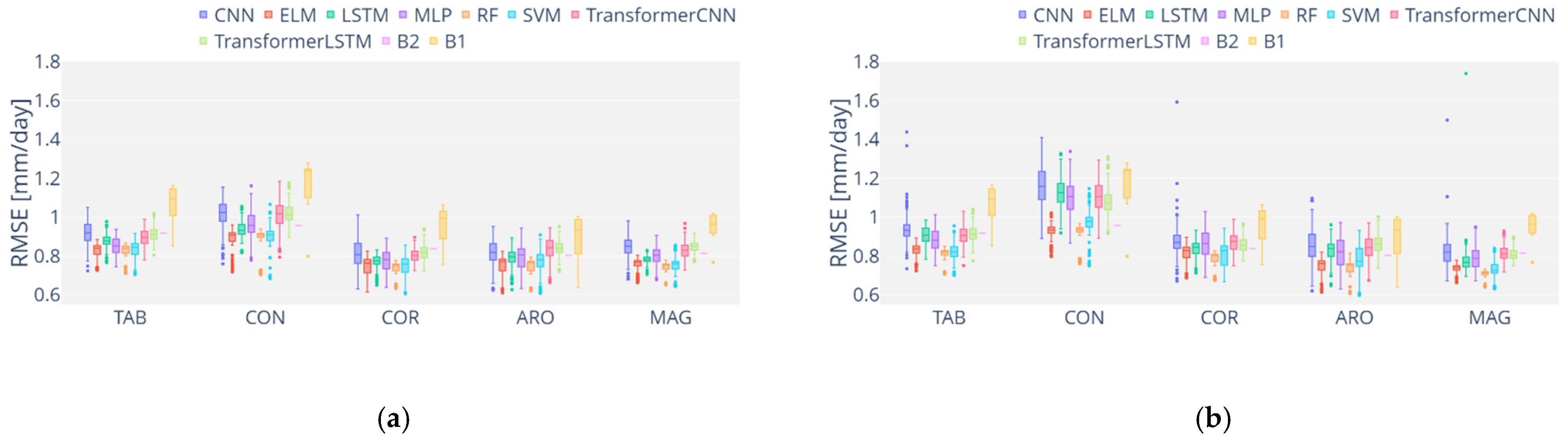
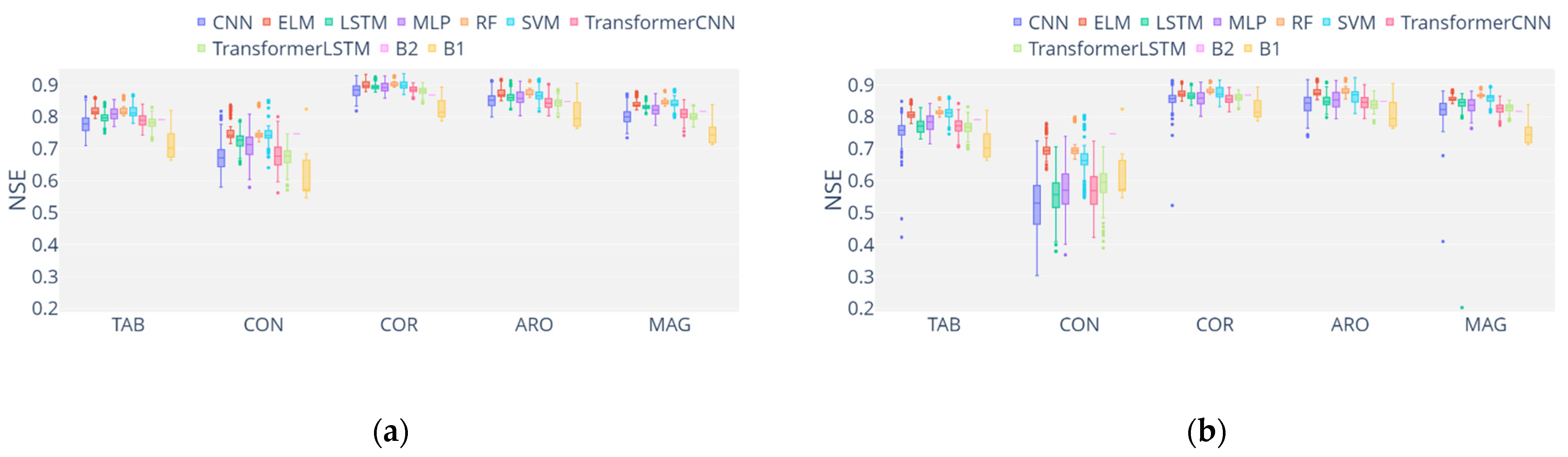
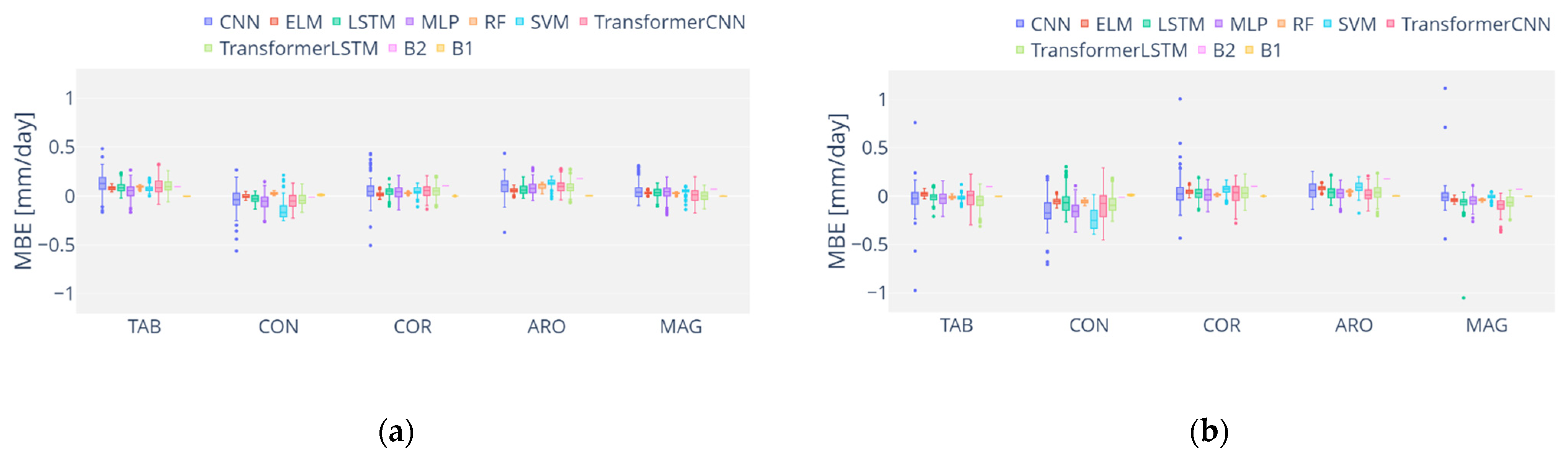
3.2. Analysis of ML Performance

Table 7. Minimum (Min.), mean, and maximum (Max.) of NSE, RMSE, and MBE values for all locations (TAB—Tabernas, CON—Conil, COR—Córdoba, ARO—Aroche, MAG—Málaga) and models using two different lag day windows (15 days and 30 days). T_CNN refers to transformer using CNN in the feed-forward layer, while T_LSTM refers to transformers using LSTM in this same layer.

Station	Model	Lag Days	NSE			RMSE			MBE
			Min	Mean	Max	Min	Mean	Max	Min	Mean	Max
TAB	CNN	15	0.710	0.778	0.862	0.723	0.916	1.050	0.001	0.123	0.484
		30	0.423	0.752	0.848	0.734	0.939	1.438	0.000	−0.026	−0.974
	ELM	15	0.794	0.820	0.860	0.727	0.825	0.885	0.043	0.082	0.126
		30	0.778	0.807	0.853	0.722	0.830	0.892	−0.000	0.021	0.079
	LSTM	15	0.749	0.797	0.845	0.766	0.877	0.976	−0.003	0.088	0.236
		30	0.730	0.771	0.828	0.783	0.905	0.984	0.000	−0.009	−0.209
	MLP	15	0.769	0.810	0.854	0.743	0.848	0.936	0.000	0.046	0.265
		30	0.715	0.781	0.841	0.750	0.883	1.012	−0.000	−0.029	−0.210
	RF	15	0.802	0.821	0.867	0.710	0.823	0.866	0.057	0.094	0.117
		30	0.799	0.819	0.859	0.706	0.805	0.850	0.000	−0.011	−0.033
	SVM	15	0.779	0.817	0.869	0.704	0.831	0.915	0.000	0.074	0.183
		30	0.746	0.812	0.862	0.700	0.818	0.955	0.000	−0.018	0.121
	T_CNN	15	0.742	0.789	0.840	0.779	0.893	0.989	0.000	0.100	0.324
		30	0.705	0.770	0.841	0.750	0.905	1.029	−0.000	−0.017	−0.297
	T_LSTM	15	0.726	0.780	0.829	0.804	0.912	1.019	0.002	0.099	0.257
		30	0.699	0.765	0.831	0.775	0.916	1.040	0.000	−0.050	−0.312
CON	CNN	15	0.580	0.674	0.817	0.759	1.017	1.154	0.000	−0.037	−0.560
		30	0.303	0.520	0.724	0.889	1.164	1.409	0.002	−0.151	−0.706
	ELM	15	0.716	0.753	0.837	0.717	0.885	0.959	0.000	0.000	0.048
		30	0.635	0.697	0.779	0.796	0.927	1.021	−0.002	−0.057	−0.122
	LSTM	15	0.651	0.724	0.788	0.816	0.936	1.055	0.000	−0.029	−0.131
		30	0.378	0.552	0.706	0.919	1.126	1.326	0.000	−0.061	0.304
	MLP	15	0.579	0.709	0.808	0.778	0.959	1.160	0.000	−0.059	−0.260
		30	0.368	0.573	0.738	0.866	1.099	1.338	0.003	−0.153	−0.371
	RF	15	0.721	0.754	0.843	0.703	0.883	0.939	0.003	0.026	0.057
		30	0.667	0.704	0.799	0.759	0.915	0.967	−0.020	−0.054	−0.099
	SVM	15	0.640	0.752	0.851	0.684	0.885	1.065	0.000	−0.146	−0.250
		30	0.547	0.672	0.804	0.749	0.961	1.146	0.015	−0.235	−0.393
	T_CNN	15	0.561	0.679	0.800	0.794	1.008	1.184	0.000	−0.047	−0.225
		30	0.422	0.569	0.723	0.891	1.104	1.294	−0.001	−0.096	−0.451
	T_LSTM	15	0.570	0.674	0.746	0.895	1.018	1.177	0.000	−0.035	−0.166
		30	0.389	0.588	0.707	0.917	1.080	1.310	0.000	−0.082	−0.259
COR	CNN	15	0.818	0.882	0.929	0.630	0.808	1.011	0.000	0.056	−0.505
		30	0.522	0.853	0.913	0.670	0.873	1.592	0.000	0.035	1.003
	ELM	15	0.879	0.900	0.932	0.614	0.745	0.824	0.000	0.015	0.084
		30	0.848	0.874	0.909	0.686	0.813	0.896	−0.001	0.046	0.128
	LSTM	15	0.877	0.894	0.924	0.649	0.771	0.831	0.000	0.041	0.178
		30	0.835	0.865	0.902	0.713	0.841	0.932	0.000	0.027	0.193
	MLP	15	0.858	0.893	0.927	0.639	0.773	0.891	−0.000	0.038	0.211
		30	0.801	0.858	0.908	0.690	0.860	1.029	−0.001	0.011	0.172
	RF	15	0.892	0.903	0.928	0.633	0.734	0.776	0.011	0.029	0.045
		30	0.870	0.883	0.912	0.674	0.783	0.826	0.000	0.015	0.033
	SVM	15	0.869	0.900	0.934	0.605	0.744	0.855	−0.000	0.053	0.130
		30	0.832	0.875	0.914	0.667	0.809	0.942	0.000	0.064	0.167
	T_CNN	15	0.857	0.885	0.906	0.725	0.802	0.896	0.003	0.052	0.207
		30	0.815	0.855	0.892	0.749	0.870	0.988	0.000	0.023	−0.280
	T_LSTM	15	0.842	0.880	0.906	0.724	0.818	0.939	−0.000	0.048	0.204
		30	0.824	0.859	0.885	0.773	0.859	0.965	0.000	0.037	0.230
ARO	CNN	15	0.799	0.851	0.913	0.624	0.816	0.951	0.000	0.106	0.436
		30	0.737	0.840	0.916	0.620	0.851	1.097	0.001	0.056	0.256
	ELM	15	0.850	0.874	0.917	0.609	0.751	0.823	−0.001	0.056	0.113
		30	0.853	0.878	0.918	0.613	0.744	0.819	0.020	0.082	0.141
	LSTM	15	0.823	0.860	0.912	0.627	0.792	0.892	0.000	0.068	0.196
		30	0.798	0.850	0.908	0.647	0.827	0.960	−0.002	0.038	0.220
	MLP	15	0.803	0.861	0.911	0.632	0.789	0.943	−0.001	0.079	0.288
		30	0.793	0.853	0.913	0.630	0.815	0.972	0.000	0.020	0.164
	RF	15	0.860	0.877	0.914	0.620	0.742	0.794	0.022	0.098	0.139
		30	0.855	0.883	0.920	0.606	0.730	0.814	0.009	0.047	0.070
	SVM	15	0.817	0.869	0.918	0.607	0.764	0.908	−0.003	0.136	0.200
		30	0.810	0.868	0.922	0.597	0.772	0.931	0.006	0.091	0.201
	T_CNN	15	0.802	0.845	0.902	0.664	0.834	0.945	0.002	0.099	0.281
		30	0.794	0.845	0.901	0.674	0.840	0.970	0.000	0.018	0.210
	T_LSTM	15	0.800	0.843	0.885	0.719	0.840	0.950	0.000	0.089	0.278
		30	0.780	0.838	0.882	0.736	0.859	1.001	0.000	0.042	0.238
MAG	CNN	15	0.734	0.800	0.871	0.681	0.847	0.980	0.000	0.046	0.311
		30	0.409	0.819	0.880	0.672	0.823	1.499	0.000	−0.003	1.113
	ELM	15	0.821	0.841	0.878	0.662	0.756	0.804	0.000	0.031	0.071
		30	0.841	0.857	0.884	0.663	0.736	0.777	−0.001	−0.040	−0.084
	LSTM	15	0.810	0.830	0.862	0.705	0.782	0.828	0.000	0.036	0.132
		30	0.202	0.840	0.872	0.695	0.773	1.739	0.000	−0.069	−1.052
	MLP	15	0.773	0.823	0.872	0.678	0.798	0.904	0.000	0.036	0.195
		30	0.763	0.835	0.880	0.672	0.788	0.948	0.000	−0.048	−0.261
	RF	15	0.832	0.849	0.882	0.651	0.738	0.778	0.000	0.027	0.044
		30	0.859	0.869	0.892	0.640	0.704	0.732	−0.020	−0.039	−0.061
	SVM	15	0.797	0.843	0.885	0.643	0.750	0.855	0.000	0.049	−0.138
		30	0.814	0.858	0.894	0.631	0.731	0.839	0.000	−0.006	−0.094
	T_CNN	15	0.741	0.809	0.853	0.727	0.829	0.967	0.001	0.009	0.198
		30	0.773	0.825	0.864	0.716	0.812	0.928	0.002	−0.097	−0.371
	T_LSTM	15	0.768	0.801	0.835	0.771	0.846	0.916	0.000	0.001	−0.130
		30	0.787	0.827	0.852	0.749	0.808	0.897	0.000	−0.063	−0.247

shows the minimum, mean, and maximum NSE, RMSE, and MBE values for all the sites and models using two different lag intervals (15 and 30 days). Generally, in terms of NSE and RMSE, the use of 15 days slightly outperformed all the models using 30 lag days for almost all the cases. On the other hand, the MBE performance for all models, locations, and lag days was very similar. Additionally, ML approaches highly outperformed the baselines, although the CNN and the transformer-based models gave the worst results in all sites. In Tabernas, the most arid site, in terms of NSE and RMSE, all the ML models surpassed the baseline performance. SVM obtained the best values (NSE = 0.869 and RMSE = 0.700 mm/day), followed very closely by RF (NSE = 0.867 and RMSE = 0.706 mm/day), which outperformed, on average, the rest of the models. On the other hand, the CNN model obtained the worst modeling for 30 lag days (NSE = 0.423 and RMSE = 1.438 mm/day). All the models obtained high mean MBE metrics, obtaining the highest MBE value (−0.974 mm/day) using CNN and 30 lag days. In Conil, the best values were obtained by SVM (RMSE = 0.684 mm/day), RF (RMSE = 0.703 mm/day), and ELM (RMSE = 0.717 mm/day), in this order and for 15 lag days. In terms of NSE, these three models also gave the best performance on mean values and for 15 lag days, whereas the worst were obtained by CNN (NSE = 0.520) for 30 lag days. In Córdoba, SVM and ELM using 15 lag days outperformed the rest of the models in both RMSE (0.605 and 0.614 mm/day) and NSE (0.934 and 0.932), respectively. Moreover, on average, the best results were obtained in Córdoba compared to the rest of the sites (NSE > 0.85, RMSE < 0.80 mm/day, and MBE ≈ 0.0 mm/day). In Aroche, the most humid site, the NSE values ranged from 0.737 (CNN model) to 0.922 (SVM model) and the RMSE values ranged from 0.597 mm/day (SVM model) to 1.097 mm/day (CNN model). Finally, in Málaga, the results using 30 lag days were slightly better for all models. SVM and RF outperformed the rest of the models in terms of NSE (0.894 and 0.892, respectively) and RMSE (0.631 mm/day and 0.640 mm/day, respectively), whereas the worst results were obtained using CNN (NSE = 0.409 and RMSE = 1.499 mm/day) and LSTM (NSE = 0.202 and RMSE = 1.739 mm/day).

In Figure 10, Figure 11 and Figure 12, the RMSE and NSE values for all forecasting predictions in the different sites are shown in a boxplot, respectively. Firstly, no significant performance distinctions were observed from the two approaches depending on the number of lag days (15 and 30 days). However, the first approach (15 lag days) slightly outperformed the second (30 lag days) on mean values, and more precision was observed (a lower interquartile range). Moreover, the number of outliers having non-accurate modeling was much higher using the second approach. Then, as a general rule, using daily values from 15 days in the past is recommended over using 30 days. Furthermore, regarding the efficiency of different models, SVM, RF, and ELM were predominantly better than the rest of the models according to NSE and RMSE values, giving more precise results. In contrast, CNN and both transformer models were at the bottom in the ranking. Finally, the MBE results are plotted in a boxplot. The results were very accurate in both approaches and for all the models and sites, but CNN gave more outliers, especially using the 30 lag days approach.

To further analyze these results, Figure 13, Figure 14 and Figure 15 show the best statistic values (NSE, RMSE, and MBE, respectively) of all the models and sites for the different forecast horizons used. In terms of NSE (Figure 13), all ML models highly outperformed B1 and B2 in all the forecast horizons and locations, except for Conil. In Conil, only SVM, RF, and ELM outperformed both B1 and B2 in all cases. On the other hand, the transformers, CNN, and MLP models underperformed B1 and B2 for a horizon higher than 3 days. Regarding RMSE, the results were similar to those shown in Figure 12. However, a more significant improvement in ML models is appreciated for most models and horizons. In terms of MBE (Figure 13, Figure 14 and Figure 15), B2 obtained significantly worse results in Aroche, Córdoba, Málaga, and Tabernas, where ML performed very accurately in all cases. In Conil, there were no major differences in performance between all the models. Thereby, due to these results, it could be stated that the use of ML models to forecast ET₀ up to a week is highly recommended, especially SVM, RF, and ELM models. Generally, B1 highly outperformed B2 to forecast ET₀ values one day ahead, but its performance profoundly decreased for higher horizons, obtaining even worse results than B2. This denotes a low autocorrelation of daily ET₀ values but a higher relation with historical monthly values. Moreover, SVM generally showed the best performance in terms of NSE and RMSE, whereas, regarding MBE, all models performed very accurately. Finally, it is worth noting that in Conil (a coastal site with an aridity index close to being a dry sub-humid climate), the best ML models (SVM, RF, and ELM) could not highly outperform B2 as in the rest of the locations when forecasting more than two days ahead, due to the effect of the close distance to the sea and the higher aridity index.

3.3. Assessing the Different Configurations

In order to evaluate the performance of the different configurations at all locations,

Table 8. Mean and minimum RMSE values (mm/day) for the different configurations at each location. The format is: mean (minimum). The best values are in bold.

Conf.	TAB	CON	COR	ARO	MAG	Mean
I	0.806 (0.704)	0.886 (0.695)	0.720 (0.614)	0.686 (0.605)	0.724 (0.648)	0.764
II	0.801 (0.709)	0.909 (0.697)	0.718 (0.618)	0.703 (0.615)	0.732 (0.631)	0.772
III	0.786 (0.701)	0.920 (0.694)	0.710 (0.633)	0.693 (0.603)	0.730 (0.643)	0.767
IV	0.794 (0.703)	0.897 (0.694)	0.724 (0.630)	0.693 (0.604)	0.734 (0.646)	0.768
V	0.812 (0.706)	0.914 (0.700)	0.741 (0.621)	0.704 (0.598)	0.732 (0.632)	0.780
VI	0.812 (0.709)	0.870 (0.687)	0.720 (0.622)	0.725 (0.602)	0.743 (0.645)	0.774
VII	0.805 (0.703)	0.902 (0.689)	0.728 (0.621)	0.710 (0.601)	0.733 (0.648)	0.775
VIII	0.805 (0.709)	0.925 (0.693)	0.737 (0.617)	0.717 (0.606)	0.725 (0.642)	0.781
IX	0.799 (0.708)	0.883 (0.694)	0.735 (0.642)	0.693 (0.613)	0.726 (0.639)	0.767
X	0.803 (0.704)	0.897 (0.699)	0.734 (0.620)	0.687 (0.613)	0.730 (0.641)	0.770
XI	0.811 (0.709)	0.931 (0.698)	0.740 (0.617)	0.686 (0.597)	0.702 (0.640)	0.774
XII	0.823 (0.712)	0.926 (0.697)	0.732 (0.640)	0.706 (0.605)	0.722 (0.641)	0.781
XIII	0.814 (0.708)	0.933 (0.691)	0.734 (0.605)	0.726 (0.615)	0.737 (0.642)	0.788
XIV	0.809 (0.714)	0.892 (0.688)	0.737 (0.643)	0.721 (0.615)	0.741 (0.643)	0.780
XV	0.811 (0.708)	0.899 (0.715)	0.730 (0.614)	0.698 (0.612)	0.721 (0.645)	0.771
XVI	0.824 (0.709)	0.904 (0.693)	0.722 (0.619)	0.706 (0.599)	0.736 (0.633)	0.778
XVII	0.810 (0.708)	0.921 (0.691)	0.753 (0.615)	0.726 (0.599)	0.734 (0.633)	0.788
XVIII	0.805 (0.707)	0.904 (0.718)	0.729 (0.622)	0.719 (0.606)	0.735 (0.647)	0.778
XIX	0.803 (0.707)	0.905 (0.688)	0.736 (0.616)	0.711 (0.605)	0.722 (0.633)	0.775
XX	0.816 (0.713)	0.879 (0.695)	0.733 (0.610)	0.719 (0.604)	0.747 (0.642)	0.778
XXI	0.801 (0.700)	0.920 (0.721)	0.725 (0.623)	0.696 (0.608)	0.738 (0.643)	0.776
XXII	0.792 (0.709)	0.893 (0.698)	0.728 (0.615)	0.709 (0.609)	0.722 (0.637)	0.768
XXIII	0.803 (0.713)	0.904 (0.696)	0.719 (0.627)	0.705 (0.604)	0.786 (0.643)	0.783
XXIV	0.823 (0.709)	0.917 (0.695)	0.741 (0.640)	0.696 (0.608)	0.731 (0.635)	0.781
XXV	0.821 (0.711)	0.863 (0.691)	0.720 (0.618)	0.714 (0.613)	0.733 (0.655)	0.770
XXVI	0.822 (0.713)	0.894 (0.684)	0.736 (0.615)	0.711 (0.605)	0.730 (0.647)	0.778
XXVII	0.803 (0.710)	0.917 (0.699)	0.714 (0.627)	0.718 (0.612)	0.734 (0.636)	0.777

shows the average and best RMSE values of each configuration in the different sites. In Tabernas, configurations III, XXII, IV, and IX obtained the most accurate results on mean, whereas configurations XVI, XII, and XXIV were the worst. In Conil, the best configurations in terms of mean RMSE were XXV, VI, and XX. Furthermore, configuration XXVI obtained the best value in absolute terms. On the other hand, configurations XIII, XI, and XII performed the worst on average. In Córdoba, regarding mean values, configurations XVII, XXIV, and V were at the bottom, whereas configurations III, XXVII, and II were at the top of the ranking. In Aroche, configuration V obtained the lowest RMSE value (RMSE = 0.598 mm/day). Moreover, considering the mean values, all configurations obtained very similar performance, beginning with RMSE = 0.764 mm/day (configuration I), followed closely by configurations IV (RMSE = 0.764 mm/day), III (RMSE = 0.767 mm/day), IX (RMSE = 0.767 mm/day), and XXII (RMSE = 0.768 mm/day), and finally RMSE = 0.788 mm/day (configurations XIII and XVII). Thus, it could be stated that in terms of the mean, although there were no significant differences in performance between the best and worst configurations, the use of configurations I, III, IV, and IX is recommended.

3.4. Overall Discussion

In this work, several aspects were evaluated in forecasting daily ET₀ at five locations in the Andalusia region (Southern Spain) with different geo-climatic conditions. Firstly, a new state-of-the-art architecture for NLP problems was assessed to forecast daily ET₀, the transformers. Specifically, two different approaches were evaluated, TransformerCNN and TransformerLSTM, and they were compared to standard machine learning models such as MLP, SVM, RF, or CNN, among others. In general, the results obtained using standard machine learning approaches such as RF, SVM, and ELM highly outperformed the rest of the models assessed in this work. Moreover, transformer-based models did not perform as expected in all cases when compared to standard ML models. However, their results were better than the baselines for most sites and cases (except for Conil). Secondly, another critical aspect to highlight in this work is that even using a self-attention mechanism (transformer-based models), the use of 30 lag days instead of 15 lag days was not beneficial to forecasting daily ET₀. On the contrary, slightly better results were obtained when 15 lag days were used, along with fewer serious outliers. Moreover, when comparing the different feature input configurations proposed in this study, none of them predominantly outperformed the rest, although configurations XIII, XIV, XX, and XXI were better on average. Figure 16, Figure 17 and Figure 18 show a scatter plot of measured vs. predicted ET₀ values using the best ML model and configuration for 1 and 7 days ahead.

Furthermore, the results of the proposed models were significantly better than those reported by Ferreira and da Cunha [18] in terms of RMSE and NSE using different deep learning approaches in Brazil in AWS with an aridity index ranging from 0.3 to 1.6. The best NSE performances in Brazil ranged from 0.35 to 0.62 (approximately), whereas in this work, the best NSE values ranged from 0.60 to 0.95 (approximately). Moreover, this work also obtained slightly better NSE values than those reported by Nourani et al. [17] using ensemble modeling in different weather stations from Iran, Turkey, and Cyprus. These previous works used temperature, relative humidity, solar radiation, and wind speed values as input features, whereas all the configurations of this work were temperature-based variables. Additionally, comparing the results to those obtained by de Oliveira and Lucas et al. [54], the assessed models in the present work outperformed their CNN and ensemble CNN results in Brazil.

In all, the models developed in this work, especially SVM, ELM, and RF, are able to accurately forecast ET₀ for one week ahead using only temperature-based parameters and ET₀ past values. This issue is vital for improving crop irrigation scheduling, allowing adequate and anticipated planning, and contributing to agricultural production. Furthermore, providing reliable ET₀ future values positively impacts the current challenge of optimizing water resource management, especially in arid and semiarid locations.

4. Conclusions

In this work, several machine learning models have been developed and assessed for daily ET₀ forecasting from 1 to 7 days ahead using different input configurations, as well as different lag days. In general, all the ML approaches outperformed the baselines for all the forecast horizons and most locations, but SVM, RF, and ELM highly outperformed the rest of the models evaluated for most sites except for Conil de la Frontera, with unusually low wind speed values in this region. On the other hand, the transformers were, on average, at the bottom of the ranking. Moreover, all configurations obtained very similar results in terms of RMSE, but configurations I, III, IV, and IX slightly outperformed the rest. The NSE values were above 0.85 for Conil, Tabernas, and Málaga and above 0.9 for Córdoba and Aroche for their best modeling. In terms of RMSE, the average performance for Tabernas was 0.92 mm/day, 1.00 mm/day for Conil, 0.81 mm/day for Córdoba, 0.80 mm/day for Aroche, and 0.78 mm/day for Málaga. This denotes a relationship in performance regarding the aridity index and the distance to the sea. For inland locations, the higher the aridity index, the lower the error of forecasting ET₀ will be. On the other hand, for coastal sites, the higher the aridity index, the higher the error. Regarding MBE, most stations and models obtained very accurate values on average for most cases, with a mean performance value of 0.011 mm/day.

Further studies can deeply explore using these models in new regions with different geo-climatic conditions, different scenarios (a different time interval and a regional scenario), and for other parameters, such as solar radiation or precipitation. Moreover, accurate feature selection or reduction could be researched because, as could be stated based on the present results, the configurations containing the worst related features based on Pearson correlation (HTx, HTn, HSr-HTn) obtained very accurate minimum and mean RMSE (Table 8 and Figure 2). The approaches proposed in this work may result in greater efficiency for optimizing water resources, improving irrigation scheduling, and anticipating the decision-making for agricultural goals. Finally, the creation of an open-source repository will allow novel scientists to apply these models using their own datasets, as well as experienced scientists to commit improvements with new features and architectures. Overall, the ultimate aim is to democratize the use of machine learning to more efficiently solve today’s agricultural problems.

References

1. FAO. The State of Food Security and Nutrition in the World 2021; FAO: Rome, Italy, 2021. [Google Scholar] [CrossRef]
2. Allen, R.; Pereira, L.; Smith, M. Crop Evapotranspiration-Guidelines for Computing Crop Water Requirements-FAO Irrigation and Drainage; FAO: Rome, Italy, 1998; Volume 56. [Google Scholar]
3. Kwon, H.; Choi, M. Error Assessment of Climate Variables for FAO-56 Reference Evapotranspiration. Meteorol. Atmos. Phys. 2011, 112, 81–90. [Google Scholar] [CrossRef]
4. Estévez, J.; García-Marín, A.P.; Morábito, J.A.; Cavagnaro, M. Quality assurance procedures for validating meteorological input variables of reference evapotranspiration in mendoza province (Argentina). Agric. Water Manag. 2016, 172, 96–109. [Google Scholar] [CrossRef]
5. Jabloun, M.; Sahli, A. Evaluation of FAO-56 Methodology for Estimating Reference Evapotranspiration Using Limited Climatic Data. Application to Tunisia. Agric. Water Manag. 2008, 95, 707–715. [Google Scholar] [CrossRef]
6. Estévez, J.; Gavilán, P.; Giráldez, J.V. Guidelines on Validation Procedures for Meteorological Data from Automatic Weather Stations. J. Hydrol. 2011, 402, 144–154. [Google Scholar] [CrossRef] [Green Version]
7. Estévez, J.; Padilla, F.L.; Gavilán, P. Evaluation and Regional Calibration of Solar Radiation Prediction Models in Southern Spain. J. Irrig. Drain. Eng. 2012, 138, 868–879. [Google Scholar] [CrossRef]
8. WMO. Guide to Instruments and Methods of Observations; WMO: Geneva, Switzerland, 2018; Volume 8, ISBN 978-92-63-10008-5. [Google Scholar]
9. George, H.H.; Zohrab, A. Samani Reference Crop Evapotranspiration from Temperature. Appl. Eng. Agric. 1985, 1, 96–99. [Google Scholar] [CrossRef]
10. Raziei, T.; Pereira, L.S. Estimation of ETo with Hargreaves-Samani and FAO-PM Temperature Methods for a Wide Range of Climates in Iran. Agric. Water Manag. 2013, 121, 1–18. [Google Scholar] [CrossRef]
11. Ravazzani, G.; Corbari, C.; Morella, S.; Gianoli, P.; Mancini, M. Modified Hargreaves-Samani Equation for the Assessment of Reference Evapotranspiration in Alpine River Basins. J. Irrig. Drain. Eng. 2012, 138, 592–599. [Google Scholar] [CrossRef]
12. Luo, Y.; Chang, X.; Peng, S.; Khan, S.; Wang, W.; Zheng, Q.; Cai, X. Short-Term Forecasting of Daily Reference Evapotranspiration Using the Hargreaves-Samani Model and Temperature Forecasts. Agric. Water Manag. 2014, 136, 42–51. [Google Scholar] [CrossRef]
13. Karimi, S.; Shiri, J.; Marti, P. Supplanting Missing Climatic Inputs in Classical and Random Forest Models for Estimating Reference Evapotranspiration in Humid Coastal Areas of Iran. Comput. Electron. Agric. 2020, 176, 105633. [Google Scholar] [CrossRef]
14. Ferreira, L.B.; da Cunha, F.F. New Approach to Estimate Daily Reference Evapotranspiration Based on Hourly Temperature and Relative Humidity Using Machine Learning and Deep Learning. Agric. Water Manag. 2020, 234, 106113. [Google Scholar] [CrossRef]
15. Yan, S.; Wu, L.; Fan, J.; Zhang, F.; Zou, Y.; Wu, Y. A Novel Hybrid WOA-XGB Model for Estimating Daily Reference Evapotranspiration Using Local and External Meteorological Data: Applications in Arid and Humid Regions of China. Agric. Water Manag. 2021, 244, 106594. [Google Scholar] [CrossRef]
16. Wu, L.; Peng, Y.; Fan, J.; Wang, Y.; Huang, G. A Novel Kernel Extreme Learning Machine Model Coupled with K-Means Clustering and Firefly Algorithm for Estimating Monthly Reference Evapotranspiration in Parallel Computation. Agric. Water Manag. 2021, 245, 106624. [Google Scholar] [CrossRef]
17. Nourani, V.; Elkiran, G.; Abdullahi, J. Multi-Step Ahead Modeling of Reference Evapotranspiration Using a Multi-Model Approach. J. Hydrol. 2020, 581, 124434. [Google Scholar] [CrossRef]
18. Ferreira, L.B.; da Cunha, F.F. Multi-Step Ahead Forecasting of Daily Reference Evapotranspiration Using Deep Learning. Comput. Electron. Agric. 2020, 234, 106113. [Google Scholar] [CrossRef]
19. Vaswani, A.; Shazeer, N.; Parmar, N.; Uszkoreit, J.; Jones, L.; Gomez, A.N.; Kaiser, L.; Polosukhin, I. Attention Is All You Need. Adv. Neural Inf. Process. Syst. 2017, 2017, 5999–6009. [Google Scholar]
20. Wu, S.; Xiao, X.; Ding, Q.; Zhao, P.; Wei, Y.; Huang, J. Adversarial Sparse Transformer for Time Series Forecasting. Adv. Neural Inf. Process. Syst. 2020, 33, 17105–17115. [Google Scholar]
21. Wu, N.; Green, B.; Ben, X.; O’Banion, S. Deep Transformer Models for Time Series Forecasting: The Influenza Prevalence Case. arXiv 2020, arXiv:2001.08317. [Google Scholar]
22. Li, S.; Jin, X.; Xuan, Y.; Zhou, X.; Chen, W.; Wang, Y.X.; Yan, X. Enhancing the Locality and Breaking the Memory Bottleneck of Transformer on Time Series Forecasting. In Proceedings of the Advances in Neural Information Processing Systems, Vancouver, BC, Canada, 8–14 December 2019; Volume 32. [Google Scholar]
23. Unep, N.M.; London, D.T. World Atlas of Desertification. Land Degrad. Dev. 1992, 3, 15–45. [Google Scholar]
24. Bellido-Jiménez, J.A.; Estévez, J.; García-Marín, A.P. New Machine Learning Approaches to Improve Reference Evapotranspiration Estimates Using Intra-Daily Temperature-Based Variables in a Semi-Arid Region of Spain. Agric. Water Manag. 2020, 245, 106558. [Google Scholar] [CrossRef]
25. Bellido-Jiménez, J.A.; Estévez, J.; García-Marín, A.P. Assessing Neural Network Approaches for Solar Radiation Estimates Using Limited Climatic Data in the Mediterranean Sea. In Proceedings of the 3rd International Electronic Conference on Atmospheric Sciences (ECAS 2020), online, 16–30 November 2020. [Google Scholar]
26. Bellido-Jiménez, J.A.; Estévez Gualda, J.; García-Marín, A.P. Assessing New Intra-Daily Temperature-Based Machine Learning Models to Outperform Solar Radiation Predictions in Different Conditions. Appl. Energy 2021, 298, 117211. [Google Scholar] [CrossRef]
27. Estévez, J.; Gavilán, P.; García-Marín, A.P. Spatial Regression Test for Ensuring Temperature Data Quality in Southern Spain. Theor. Appl. Climatol. 2018, 131, 309–318. [Google Scholar] [CrossRef]
28. Islam, A.R.M.T.; Shen, S.; Yang, S.; Hu, Z.; Chu, R. Assessing Recent Impacts of Climate Change on Design Water Requirement of Boro Rice Season in Bangladesh. Theor. Appl. Climatol. 2019, 138, 97–113. [Google Scholar] [CrossRef]
29. Yi, Z.; Zhao, H.; Jiang, Y. Continuous Daily Evapotranspiration Estimation at the Field-Scale over Heterogeneous Agricultural Areas by Fusing Aster and Modis Data. Remote Sens. 2018, 10, 1694. [Google Scholar] [CrossRef] [Green Version]
30. Sattari, M.T.; Apaydin, H.; Band, S.S.; Mosavi, A.; Prasad, R. Comparative Analysis of Kernel-Based versus ANN and Deep Learning Methods in Monthly Reference Evapotranspiration Estimation. Hydrol. Earth Syst. Sci. 2021, 25, 603–618. [Google Scholar] [CrossRef]
31. Tikhamarine, Y.; Malik, A.; Souag-Gamane, D.; Kisi, O. Artificial Intelligence Models versus Empirical Equations for Modeling Monthly Reference Evapotranspiration. Environ. Sci. Pollut. Res. 2020, 27, 30001–30019. [Google Scholar] [CrossRef]
32. Huang, G.B.; Zhu, Q.Y.; Siew, C.K. Extreme Learning Machine: Theory and Applications. Neurocomputing 2006, 70, 489–501. [Google Scholar] [CrossRef]
33. Zhu, B.; Feng, Y.; Gong, D.; Jiang, S.; Zhao, L.; Cui, N. Hybrid Particle Swarm Optimization with Extreme Learning Machine for Daily Reference Evapotranspiration Prediction from Limited Climatic Data. Comput. Electron. Agric. 2020, 173, 105430. [Google Scholar] [CrossRef]
34. Akusok, A.; Björk, K.-M.; Miche, Y.; Lendasse, A. High Performance Extreme Learning Machines: A Complete Toolbox for Big Data Applications. IEEE Access 2015, 3, 1011–1025. [Google Scholar] [CrossRef]
35. Smola, A.J.; Schölkopf, B. A Tutorial on Support Vector Regression. Stat. Comput. 2004, 14, 199–222. [Google Scholar] [CrossRef] [Green Version]
36. Chen, Z.; Zhu, Z.; Jiang, H.; Sun, S. Estimating Daily Reference Evapotranspiration Based on Limited Meteorological Data Using Deep Learning and Classical Machine Learning Methods. J. Hydrol. 2020, 591, 125286. [Google Scholar] [CrossRef]
37. de Oliveira, R.G.; Valle Júnior, L.C.G.; da Silva, J.B.; Espíndola, D.A.L.F.; Lopes, R.D.; Nogueira, J.S.; Curado, L.F.A.; Rodrigues, T.R. Temporal Trend Changes in Reference Evapotranspiration Contrasting Different Land Uses in Southern Amazon Basin. Agric. Water Manag. 2021, 250, 106815. [Google Scholar] [CrossRef]
38. Ghimire, S.; Deo, R.C.; Raj, N.; Mi, J. Deep Solar Radiation Forecasting with Convolutional Neural Network and Long Short-Term Memory Network Algorithms. Appl. Energy 2019, 253, 113541. [Google Scholar] [CrossRef]
39. Kim, S.; Hong, S.; Joh, M.; Song, S.K. DeepRain: ConvLSTM Network for Precipitation Prediction Using Multichannel Radar Data. arXiv 2017, arXiv:1711.02316. [Google Scholar]
40. Aloysius, N.; Geetha, M. A Review on Deep Convolutional Neural Networks. In Proceedings of the 2017 IEEE International Conference on Communication and Signal Processing, ICCSP, Chenai, India, 6–8 April 2017; Institute of Electrical and Electronics Engineers Inc.: Piscataway, NJ, USA, 2018; Volume 2018, pp. 588–592. [Google Scholar]
41. Hochreiter, S.; Schmidhuber, J. Long Short-Term Memory. Neural Comput. 1997, 9, 1735–1780. [Google Scholar] [CrossRef]
42. Song, H.; Rajan, D.; Thiagarajan, J.J.; Spanias, A. Attend and Diagnose: Clinical Time Series Analysis Using Attention Models. In Proceedings of the 32th AAAI Conference on Artificial Intelligence, New Orleans, LA, USA, 2–7 February 2018. [Google Scholar]
43. Wolf, T.; Debut, L.; Sanh, V.; Chaumond, J.; Delangue, C.; Moi, A.; Cistac, P.; Rault, T.; Louf, R.; Funtowicz, M.; et al. Transformers: State-of-the-Art Natural Language Processing; Association for Computational Linguistics (ACL): Stroudsburg, PA, USA, 2020; pp. 38–45. [Google Scholar]
44. Mohammdi Farsani, R.; Pazouki, E. A Transformer Self-Attention Model for Time Series Forecasting. J. Electr. Comput. Eng. Innov. 2021, 9, 1–10. [Google Scholar] [CrossRef]
45. Alizamir, M.; Kisi, O.; Muhammad Adnan, R.; Kuriqi, A. Modelling Reference Evapotranspiration by Combining Neuro-Fuzzy and Evolutionary Strategies. Acta Geophys. 2020, 68, 1113–1126. [Google Scholar] [CrossRef]
46. Mohammadi, B.; Mehdizadeh, S. Modeling Daily Reference Evapotranspiration via a Novel Approach Based on Support Vector Regression Coupled with Whale Optimization Algorithm. Agric. Water Manag. 2020, 237, 106145. [Google Scholar] [CrossRef]
47. Gijsbers, P.; LeDell, E.; Thomas, J.; Poirier, S.; Bischl, B.; Vanschoren, J. An Open Source AutoML Benchmark. arXiv 2019, arXiv:1907.00909. [Google Scholar]
48. Kotthoff, L.; Thornton, C.; Hoos, H.; Hutter, F.; Leyton-Brown, K. Auto-WEKA 2.0: Automatic Model Selection and Hyperparameter Optimization in WEKA. J. Mach. Learn. Res. 2017, 18, 826–830. [Google Scholar]
49. Jin, H.; Song, Q.; Hu, X. Auto-Keras: An Efficient Neural Architecture Search System. In Proceedings of the 25th ACM SIGKDD International Conference on Knowledge Discovery & Data Mining, Anchorage, AK, USA, 4–8 August 2019; pp. 1946–1956. [Google Scholar]
50. Feurer, M.; Klein, A.; Eggensperger, K.; Springenberg, J.T.; Blum, M.; Hutter, F. Auto-Sklearn:: Efficient and Robust Automated Machine Learning. In Proceedings of the Advances in Neural Information Processing Systems, Montreal, QC, Canada, 7–12 December 2015; Volume 2015, pp. 2962–2970. [Google Scholar]
51. Hutter, F.; Kotthoff, L.; Vanschoren, J. (Eds.) Automated Machine Learning; The Springer Series on Challenges in Machine Learning; Springer International Publishing: Cham, Switzerland, 2019; ISBN 978-3-030-05317-8. [Google Scholar]
52. Borji, A.; Itti, L. Bayesian Optimization Explains Human Active Search. In Advances in Neural Information Processing Systems; Curran Associates, Inc.: New York, NY, USA, 2013; Volume 26. [Google Scholar]
53. Shahriari, B.; Swersky, K.; Wang, Z.; Adams, R.P.; de Freitas, N. Taking the Human Out of the Loop: A Review of Bayesian Optimization. Proc. IEEE 2016, 104, 148–175. [Google Scholar] [CrossRef] [Green Version]
54. de Oliveira e Lucas, P.; Alves, M.A.; de Lima e Silva, P.C.; Guimarães, F.G. Reference Evapotranspiration Time Series Forecasting with Ensemble of Convolutional Neural Networks. Comput. Electron. Agric. 2020, 177, 105700. [Google Scholar] [CrossRef]
Figure 1. Spatial distribution of Aroche, Conil, Córdoba, Málaga, and Tabernas in the Andalusia region, south of Spain.
Agronomy 12 00656 g001
Figure 2. Pearson correlation values of the assessed features in all the stations.
Agronomy 12 00656 g002
Figure 3. Mind map of the matrix data structure.
Agronomy 12 00656 g003
Figure 4. Forecasting approaches using configuration 1 as an example.
Agronomy 12 00656 g004
Figure 5. Methodology flowchart.
Agronomy 12 00656 g005
Figure 6. Single neuron architecture. I1, I2, I3, and I4 represent the inputs of the neuron; W1, W2, W3, and W4 correspond to the weights of every input; B is the bias, and O represents the output of the neuron after passing through an activation function.
Agronomy 12 00656 g006
Figure 7. Original transformer architecture.
Agronomy 12 00656 g007
Figure 8. Sine/cosine positional encoding for 31 days in a month (a) and 12 months in a year (b).
Agronomy 12 00656 g008
Figure 9. The architecture of the proposed multi attention-based model.
Agronomy 12 00656 g009
Figure 10. Boxplot with RMSE values from all models and configurations in the different AWS, using 15 lag days (a) and 30 lag days (b).
Agronomy 12 00656 g010
Figure 11. Boxplot with NSE values from all models and configurations in the different AWS, using 15 lag days (a) and 30 lag days (b).
Agronomy 12 00656 g011
Figure 12. Boxplot with MBE values from all models and configurations in the different AWS, using 15 lag days (a) and 30 lag days (b).
Agronomy 12 00656 g012
Figure 13. Scatter plot with the best NSE value for each model and location.
Agronomy 12 00656 g013
Figure 14. Scatter plot with the best RMSE value for each model and location.
Agronomy 12 00656 g014
Figure 15. Scatterplot with the best MBE value for each model and location.
Agronomy 12 00656 g015
Figure 16. Scatter plot for measured vs. predicted values for (a) forecast horizon 1 in Tabernas, (b) forecast horizon 1 in Conil de la Frontera, (c) forecast horizon 7 in Tabernas, and (d) forecast horizon 7 in Conil de la Frontera.
Agronomy 12 00656 g016
Figure 17. Scatter plot for measured vs. predicted values for (a) forecast horizon 1 in Aroche, (b) forecast horizon 1 in Málaga, (c) forecast horizon 7 in Aroche, and (d) forecast horizon 7 in Málaga.
Agronomy 12 00656 g017
Figure 18. Scatter plot for measured vs. predicted values for (a) forecast horizon 1 in Córdoba, (b) forecast horizon 7 in Córdoba.
Agronomy 12 00656 g018