Automatic Bunch Detection in White Grape Varieties Using YOLOv3, YOLOv4, and YOLOv5 Deep Learning Algorithms

Abstract

Over the last few years, several Convolutional Neural Networks for object detection have been proposed, characterised by different accuracy and speed. In viticulture, yield estimation and prediction is used for efficient crop management, taking advantage of precision viticulture techniques. Convolutional Neural Networks for object detection represent an alternative methodology for grape yield estimation, which usually relies on manual harvesting of sample plants. In this paper, six versions of the You Only Look Once (YOLO) object detection algorithm (YOLOv3, YOLOv3-tiny, YOLOv4, YOLOv4-tiny, YOLOv5x, and YOLOv5s) were evaluated for real-time bunch detection and counting in grapes. White grape varieties were chosen for this study, as the identification of white berries on a leaf background is trickier than red berries. YOLO models were trained using a heterogeneous dataset populated by images retrieved from open datasets and acquired on the field in several illumination conditions, background, and growth stages. Results have shown that YOLOv5x and YOLOv4 achieved an F1-score of 0.76 and 0.77, respectively, with a detection speed of 31 and 32 FPS. Differently, YOLO5s and YOLOv4-tiny achieved an F1-score of 0.76 and 0.69, respectively, with a detection speed of 61 and 196 FPS. The final YOLOv5x model for bunch number, obtained considering bunch occlusion, was able to estimate the number of bunches per plant with an average error of 13.3% per vine. The best combination of accuracy and speed was achieved by YOLOv4-tiny, which should be considered for real-time grape yield estimation, while YOLOv3 was affected by a False Positive–False Negative compensation, which decreased the RMSE.

1. Introduction

Over the last few years, the advent of Digital Agriculture (DA) exponentially increased the amount of data per hectare produced by agricultural activities. In viticulture, the implementation of site-specific management and precision viticulture technologies [1,2] increased the amount of information available to winegrowers. On the one hand, farming digitalisation footprint will affect the sustainability of farm-related activities [3,4]; on the other hand, the demand for efficient, fast, and smart data processing is rising. Artificial Intelligence (AI) makes it possible to collect and analyse a large amount of agricultural data, which might help improve yield with a lower quantity of inputs. Several decision support systems (DSSs) have been proposed over the last few years to help farmers and winegrowers manage information based on data acquired in the field and processed by specific algorithms through (AI). In machine learning (ML) techniques, which are a subset of AI, algorithms are trained to infer specific patterns based on a set of data to determine the actions needed to achieve a given goal. The ML approach can be unsupervised or supervised based on the necessity to be fed with already classified data or not. A supervised ML algorithm requires a large amount of data to set up the embedded statistical models through progressive corrections to their parameters by comparing the obtained results with the classified data in the input. In the last decade, the availability of new sensors and technologies increased the potential application of ML in viticulture. Several studies investigated the ML application in viticulture for yield estimation, assessment of shoot characteristics, vineyard management, disease detection, and evaluation of bunch compactness [5].

In ML data processing, the progressive correction of parameters aims to reduce the value of a specific function, which estimates the error model (loss function). Several loss functions can be used according to the final aim of the trained model. The most used ML techniques in agriculture include decision trees (e.g., random forest), support vector machine (SVM), and artificial neural networks (ANN) [6,7]. ANN are based on different nodes interconnected and organised in a specific topology. The number of layers and type of connection range from one, in the case of the perceptron, to multiple layers, in the case of deep neural networks (DNN) [6]. DNN are commonly referred to as Deep Learning (DL). DL comprises multilayer neural networks, which combine different algorithms to address a complex problem.

One of the most important DL models used for computer vision and image understanding is Convolutional Neural Networks (CNN). CNN are based on three types of neural layers: (i) convolutional layers, which convolve the whole image; (ii) pooling layers, which reduce the spatial dimensions of the input data for the next convolutional layer; and (iii) fully connected layers, which are the high-level reasoning layers of the neural network [8]. CNN can be used to analyse, combine, and extract colour, geometric, and texture features of images, allowing for the ability to address classification, localisation, and object detection. Object Detection is a computer vision technique that combines image classification and object localisation. The object detection models are mainly based on two different frameworks: the first is based on region proposals and the classification of each proposal into different object categories, and the second addresses object detection as a regression or classification problem [9]. Bounding boxes over the image usually compose object detection output, but some models give semantic segmentation as a final result. Examples of region proposal object detection models are R-CNN, Faster R-CNN, and Mask R-CNN, while examples of regression/classification-based models are You Only Look Once (YOLO) [10] and Single Shot Detector (SSD). Region proposal models are usually more accurate than regression/classification but slower due to the region proposal step. Regional-based Convolutional Neural Network (R-CNN) is based on three modules: (i) region proposal uses a selective search to define a set of 2000 candidate detections available to the detector, (ii) a CNN extracts a fixed-length feature vector from each region, and (iii) a set of class-specific linear support vector machines [11]. In Faster R-CNN, the region proposal module was improved to be faster, sharing full-image convolutional features with the detection layer and reducing the computational cost of region proposals [12]. Mask R-CNN is an implemented version of Faster R-CNN that allows semantic segmentation of objects with a small computational overhead [13].

On the other hand, SSD uses a single DNN to identify the output bounding boxes into a set of default boxes. During class prediction, the network estimates the probability that a class object is contained in a box [14]. SSD is composed of a series of convolution and pooling layers to generate feature maps at a different scale, predicting bounding box and object class at the same time and faster than R-CNN [15] with a competitive accuracy. YOLO models are presented in the following paragraphs.

1.1. Yield Estimation and Yield Prediction in Viticulture

Monitoring crop development and accurately estimating yield is crucial for efficient crop management [16]. The early estimation of the grapevine bunch load allows adjusting the vine’s vigour, thus promoting ripening and grape quality. Besides, yield predictions represent useful information for winery management. Nevertheless, the grape yield is influenced by several factors, such as growing area, weather and soil conditions, cultivar, rootstock, and vine heterogeneity. Conventional grape yield estimation takes advantage of climatic data and phenological information collected over the years, combined with yield components (number of bunches, number of berries, and berry weight) collected in defined sampling points. The final berry weight can be estimated by multiplying the berry weight during the lag phase (before veraison) for a definite coefficient [17]. De La Fuente [18] compared three grape yield prediction models. The first type was based on the number of bunches and historical bunch weight, the second used berry weight at veraison compared with historical berry weight at harvest, and the third based on the number of bunches and the bunch weight during the lag phase. Indeed, during the lag phase, berry weight is approximately 50% of its final weight [19]. The study of De La Fuente highlighted that the grape prediction models based on the number of bunches are characterised by an inherent error, although useful for yield early prediction. Yield monitor based on load cells can be used for yield estimation during harvesting, but early yield estimation can be performed only in the case of mechanical crops thinning in mid-season [20].

In the last decade, the introduction of precision viticulture has brought new opportunities for yield monitoring [1] and prediction, taking advantage of several proximal and remote sensors. Information about spatial variability derived from remotely sensed data was used to explore the correlation between several vegetation indices and grape yield [21]. Remotely sensed vegetation indices may be used to identify specific features of terroir and stress condition [22,23], especially considering their cost-effectiveness [24,25]. Proximal sensors are widely used in precision viticulture, and several tools exist to monitor physiological responses of vegetation [26] and yield [2]. Although optical spectral sensors may be used to estimate grape yield and its composition [21,27], three-dimensional estimation methods showed higher accuracy to estimate grape yield [28].

In the last few years, ML was applied to grape yield prediction. Several sensors can take advantage of ML algorithms, such as spectral and thermal cameras [29]. ML approaches combine colour, geometric, and texture features for better exploitation of the images acquired. Different ML algorithms were proposed for bunch and berries detection. Aquino et al. [30] used an ANN implemented on automatically acquired images for early yield prediction in vineyards. ML was also used for the evaluation of grape bunch compactness and quality, taking advantage of colour properties. Nuske et al. [31] proposed an automated computer vision method based on the shape and visual texture to identify and count green grape berries on a green leaf background. In this approach, an RGB camera was mounted on a small vehicle driven along the rows to detect berry locations. Their approach could predict yield to within 9.8% of the actual crop weight. A pixel classification algorithm based on shape, colour, and texture allowed for the detection of berries with a similar colour to the background [32]. This model for yield spatial variability estimation captured up to 75% of yield spatial variance with an average error between 3% and 11% of the total yield. An unsupervised recognition algorithm was applied by Di Gennaro et al. [33] to derive the number of bunches and their size on UAV-acquired images. Similarly, an unsupervised classification was used by [34] for identification of vines in 3D point-clouds. Santos et al. [35] used a Mask R-CNN [13] for grape detection, segmentation, and tracking, achieving excellent results (0.91 F1-score). The latter studies combined object detection with instance segmentation, thus obtaining high accuracy but low detection speed. Despite promising results achieved on yield estimation, some drawbacks still need to be addressed. Specifically, different clustering and variable lighting conditions of fruit on plants represent the major challenges limiting fruit detection and localisation accuracy [29]. Several of the mentioned authors trained their algorithm on red grape varieties due to greater ease in detection based on colour features.

1.2. YOLO (You Only Look Once) and Frameworks

Differently from other object detection algorithms previously developed, YOLO [10] addresses object detection as a single regression problem, avoiding the region proposal, classification, and duplicating elimination pipeline. Although YOLO can be used in several frameworks, Darknet represents the most used framework for YOLO below version 5 [36]. In YOLO algorithms, images are resized at a lower resolution; then, a single CNN runs on the images, giving as an output the detection results according to the model’s confidence threshold. The first version of YOLO was optimised to decrease the sum of square error (loss function). This optimisation increases the detection speed but with lower accuracy than state-of-the-art object detection models [10]. In YOLO, on-line data augmentation is implemented, increasing the variability of the input images, to improve the model robustness in object detection in different environments. YOLO models were applied in numerous applications where fast detection was needed, such as pedestrian detection [37], license plate recognition [38], and automatic detection of fabric defects [39]. In agriculture, YOLO application ranges from fruit detection [40,41,42], crop disease identification [43,44], and weed and pest identification [45,46]. The YOLO’s fruit detection application was mainly based on apple orchards, and application in vine bunch detection is still missing. Since 2016, several versions of YOLO have been released, showing a constant improvement of the algorithm. Besides, each main version was released as a full model and in tiny versions, characterised by a reduced number of layers and faster than the full version. In this study, the last three versions of YOLO (YOLOv3, YOLOv4, and YOLOv5, full and tiny versions) were compared for grapevine bunch detection.

1.3. YOLOv3

Version 3 of YOLO was released by Redmon and Farhadi [36]. YOLOv3 replaces the mean squared error of the previous YOLO version with a cross-entropy loss function. The cross-entropy function increases as the predicted probability calculated by the model diverges from the actual class. YOLOv3 takes advantage of Darknet-53 network for feature extraction, which relies on 53 convolutional layers. YOLOv3 predicts the object class for each bounding box using logistic regression instead of a softmax classifier [47]. YOLOv3 can predict boxes at different scales (small, medium, and large size) using three different YOLO classifier layers. For each of these three layers, three anchors are defined, proposing to the model aspect ratio, position, and dimension of boxes. YOLOv3-tiny is based on the Darknet-19 network, which relies on 19 convolutional neural networks. YOLOv3-tiny can predict boxes at two different scales using two YOLO classifier layers. For each of these layers, three anchors are defined. In YOLOv3 models, saturation, exposure, hue, blur, cropping, and aspect ratio data augmentation methods are available. Several authors modified the original models in terms of number and type of convolutional layers.

1.4. YOLOv4

YOLOv4 was released in April 2020 with several enhancements compared to YOLOv3. YOLOv4 was based on CSP Darknet-53. Cross-stage partial connections (CSP) divide the input features into two groups: one group is processed by the convolutional layer, while the second sidesteps the convolutional layers and is included in the input for the following layer [48]. Additional data augmentation methods are available in YOLOv4, such as mosaic and cutmix [49]. In the mosaic, an augmented image is generated by combing four input images in a specific ratio. In cutmix, a new image is created using parts of input images. YOLOv4 has more layers compared to the previous versions. The loss function of YOLOv4 models is a Complete-IoU, which optimises the overlap area, central point distance, and aspect ratio of predicted bounding boxes [50]. In YOLOv4-tiny, the number of layers is compressed, and only two YOLO classifiers are used (both with three anchor boxes).

1.5. YOLOv5

YOLOv5 was released in May 2020 by Jocher et al. [51] from Ultralytics LLC (Los Angeles, CA – USA), a different developer from the previous YOLO versions. Although there were some controversies related to the definition as a new YOLO version, YOLOv5 was accepted by the deep learning community [52]. The main advantage of YOLOv5 relies on the usage of the Python language instead of C. The native framework for YOLOv5 is PyTorch, which allows for faster training [51]. In terms of performance metrics, YOLOv5 allows rapid detection with the same accuracy as YOLOv4 [53]. Similarly, from the previous versions, YOLOv5 was released in different sizes (s, m, l, and x) with different accuracy and speed of detection.

According to the presented features, YOLOv3, YOLOv4, and YOLOv5 models are characterised by a different dimension (number of layers and complexity), average accuracy, speed of detection, and training. Numerous applications of YOLO were proposed for fruit detection [42,43,44,45], but a limited number of studies investigated on the YOLO application for grapevine bunch detection [35]. In the current study, a comparison of YOLOv3, YOLOv4, and YOLOv5 models for automatic bunch detection in white grapevine was carried out. Indeed, white grape varieties are characterised by colour features similar to the surrounding leaf background. In this environment, the grape bunch detection becomes much more complex but potentially applicable in the early stages after blooming in any varieties (before the berry veraison). For each version, the full model and its tiny version were evaluated. In YOLOv5 the “x” and the “s” version were evaluated. The framework and the training dataset were presented. A new open dataset for bunch image was then described. The trained models were evaluated on an external dataset (validation) in terms of accuracy and number of the object identified. Finally, the potential application of these models was described.

2. Materials and Methods

Darknet framework was used for YOLOv3 and YOLOv4 training, while Pytorch was used for YOLOv5. Data processing and analysis were performed in Google Colaboratory (Colab). In this study, Colab Pro version was used due to the elevated computational demand and the long virtual machine lifetime required for training a neural network. Training and detection tasks were performed, taking advantage of a Tesla P100 GPU (NVIDIA, Santa Clara, CA, USA) with CUDA parallel computing platform version 10.1 and 16 GB of dedicated random-access memory (RAM). The operating system of the virtual machines used for the current study was Ubuntu version 18.04.5 LTS. All Colab analyses were performed with the Python 3 programming language. The cuDNN 7.6.5 library [54] was used to take advantage of GPU acceleration.

2.1. Data Collection and Labelling

Training and evaluating a neural network for object detection requires a large number of labelled images. Several labelled-image datasets are available for benchmark, research, and commercial use, such as PASCAL, COCO, or ImageNet. To the best of the authors’ knowledge, only a few open datasets contain labelled images of white grapes. Open Image Dataset v6 (OIDv6) [55] is a dataset of labelled images for classification, segmentation, localisation, and object detection. OIDv6 contains 16 million bounding boxes for 600 object classes on 1.9 million images. White grape images, preferably acquired in the field condition, were selected from this dataset. GrapeCS-ML [5] dataset archives images of 15 different grape varieties at different phenological stages, together with chemical analysis for grape quality and maturity. GrapeCS-ML consists of 2078 images, some of them including size and Macbeth colour references. For the aim of this study, white grape variety images were selected (Viognier, Riesling, Sultana, Sauvignon Blanc, and Chardonnay) from the GrapeCS-ML dataset since all the white grape varieties were contained in this dataset. The final dataset used in this study was composed of images collected from OIDv6 and GrapeCS-ML, with the addition of field images acquired by the authors in six experimental vineyards located in different Italian regions (Lombardy, Veneto, and Marche) during the 2020 growing season. The dataset was mainly composed of images acquired on Chardonnay, Glera, and Trebbiano varieties. A set of 61 images was acquired in a vineyard from the University of Padova, characterised by several varieties, which were not identified.

The dataset used for the model training was composed of 2931 images, divided into two sets of data: Train, and Test data, which represented 66.6% and 33.3%, respectively, of the images used during the training process. Besides, 54 images with the actual number of bunches recorded were selected as the external validation dataset, used to assess the models’ performances. The external validation dataset was selected in order to reduce the effect of overfitting on the test dataset during the validation.

Table 1. Dataset composition for train, test, and validation.

Set	Number of Images
Train	1954
Test	977
Validation	54
Total	2985

summarises the final dataset composition. The result of models validated using an external validation dataset makes the validation more solid for the real application in the field, even if the validation metrics are lower.

Data annotation (known as labelling) is a fundamental component of deep learning, and it directly affects the learning capacity of the models [9]. The images collected from the dataset mentioned above were manually labelled, drawing bounding boxes on each bunch in the image using the Yolo_label V2 project [56]. Yolo_label allows for the creation of an annotation (label) for the object detection algorithm using the Yolo label format, which consists of five columns for each object (object-class, x, y, width, and height). As only one class (bunches) was used to label the dataset of this study, all label text files started with 0, which is the identification of the first index in Python.

2.2. Training, Test, and Validation

YOLO models (v3, v4, and v5) were trained singularly, using the described dataset. The training processes were performed on the pre-trained weights provided by the YOLO developers. YOLOv3 and YOLOv4 were trained for 6000 epochs, while YOLOv5 was trained for 100 epochs since the different framework required fewer iterations. For each model, a specific calibration of training hyperparameters was performed. YOLO config file allows hyperparameter modification to achieve the best result during training. The first section of the config file reports the number of images used during one epoch (batch size) and the dimensions of the resampled images used during training (width and height). For YOLOv3 and YOLOv4 training and detection, a batch size of 64 images with a pixel size of 608 × 608 was used. In YOLOv5, a batch size of 16 images was used due to the higher complexity of the model. Online data augmentation was activated for YOLOv3, YOLOv4 full models, and both YOLOv5 models. Data augmentation techniques introduced in the training process unobserved data, obtained from combinations and modification of the input dataset. In the current training, images were augmented in terms of saturation and exposure using a coefficient of 1.5. Hue value was randomly augmented with a coefficient of 0.05. Moreover, blur and mosaic were randomly applied to input images.

According to this training configuration, each model was characterised by a different computational demand (expressed in billions of floating-point operations per second, BFLOPS), which was 11.64, 139.50, 14.50, 127.23, 16.40, and 217.13 for YOLOv3-tiny, YOLOv3, YOLOv4-tiny, YOLOv4, YOLOv5s, and YOLOv5x, respectively.

Table 2. Training details and hyperparameters.

Models	Epoch	Framework	Augmentation					Billions of FLOPs
				Sat. & Exp.	Hue	Blur	Mosaic
V3-tiny	6000	Darknet	Online	null				11.6
V3				1.5	0.05	yes	no	140
V4-tiny				null				14.5
V4				1.5	0.05	yes	yes	127
V5s	100	PyTorch		1.5	0.05	yes	no	16.4
V5x								217

summarises the training specification.

Several performance measures can be used to evaluate a confusion matrix obtained from a classification model on test data. In this study, F-1 score, Precision, and Recall were chosen, calculated according to Equation (1). The F-1 score represents the harmonic mean of Precision and Recall, and it was proposed by Dice [57]. Besides, mean average precision (mAP) was used as a performance metric. mAP summarises the average detection precision and represents the area under the precision–recall curve at a defined value of IoU. mAP@50 represents the area under the precision–recall curve with a grade of overlapping bounding boxes of 50%. Performance metric calculation was evaluated on the Test and the Validation datasets. Confusion matrix and performance metrics were calculated using functions implemented in Darknet and PyTorch. The comparison and graphs were carried out using GraphPad Prism 8.0.2 (GraphPad Software, Inc., San Diego, CA, USA) and Microsoft Excel (Microsoft Corporation, Redmond, WA, USA).

$$\begin{gathered} F1\text{-}score=2\times \frac{Precision\times Recall}{Precision+Recall} \\ \mathrm{where} \\ Precision=\frac{True Positive}{True Positive+False Negative} \mathrm{and} Recall=\frac{True Positive}{True Positive+False Positive} \end{gathered}$$

(1)

The Validation dataset was finally used to compare bunch detection. The real number of bunches estimated was evaluated, taking advantage of the actual number of bunches counted in the field in the Validation dataset.

3. Results

The training process was carried out on each YOLO model, taking advantage of the presented configuration. During the training, the models’ performances were automatically estimated on the test dataset. The mAP@50 were calculated at different epoch intervals (100 in Darknet and 1 in PyTorch). Last mAP@50, best mAP@50 achieved during the training, and other performance metrics (precision, recall, and F1) are reported in

Table 3. Quantitative results of the training process.

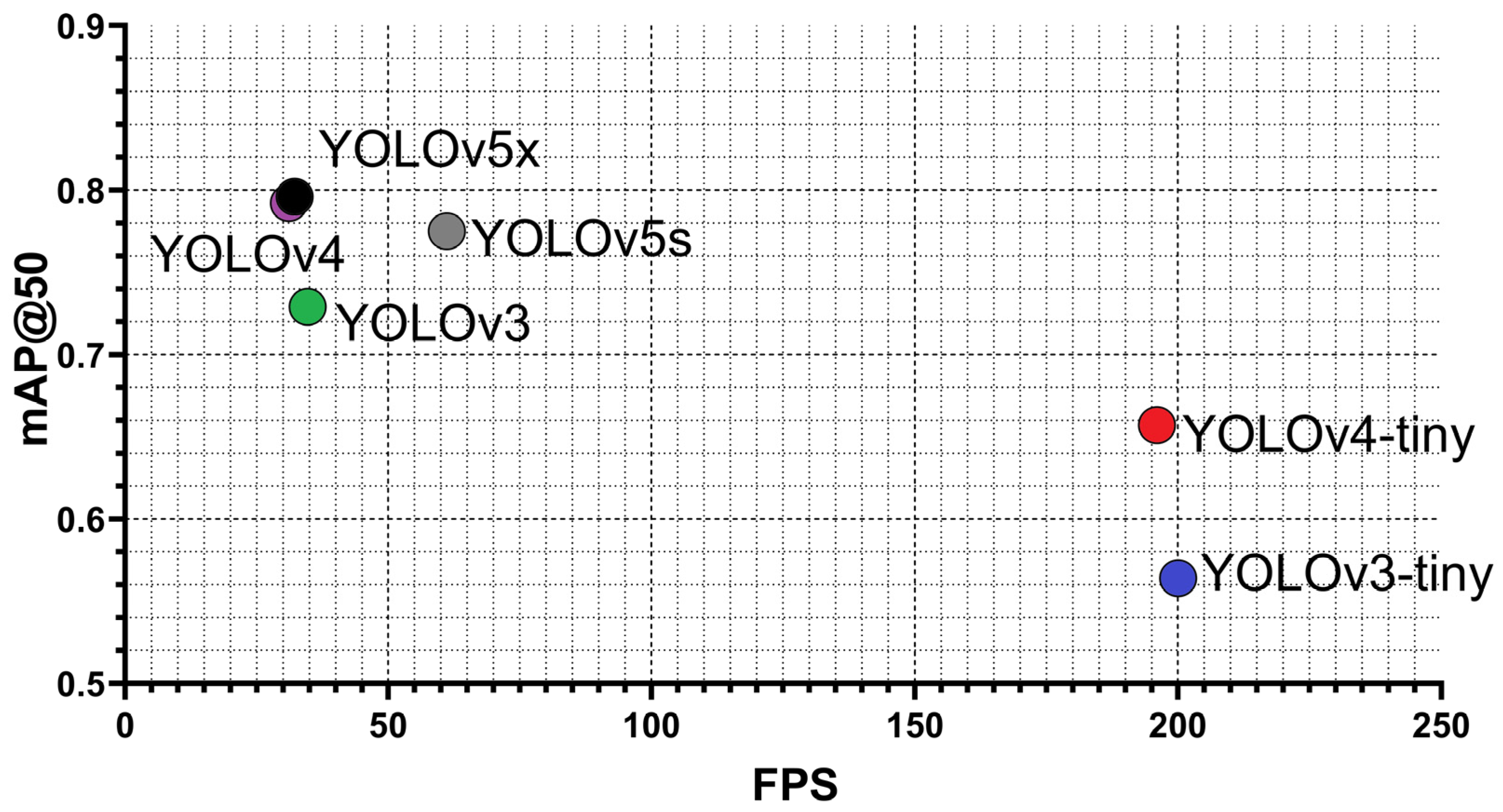
Models	Training Time (h)	Last mAP@50	Best mAP@50	Precision	Recall	F1-Score
V3-tiny	3.48	53.7%	54.4%	0.71	0.45	0.55
V3	15.2	69.2%	69.9%	0.79	0.61	0.69
V4-tiny	3.66	62.9%	63.2%	0.75	0.53	0.63
V4	16.4	71.9%	73.2%	0.76	0.69	0.72
V5s	4.66	69.5%	73.1%	0.74	0.70	0.72
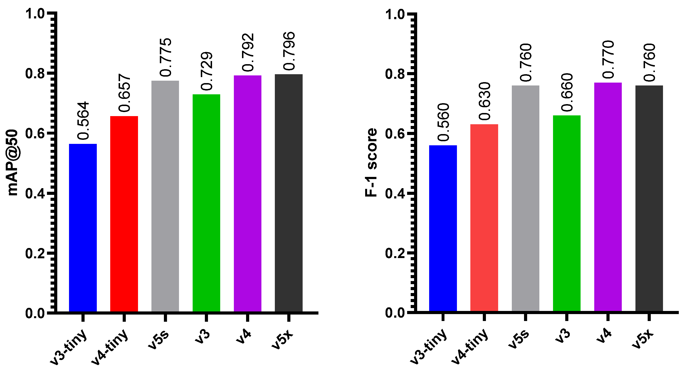
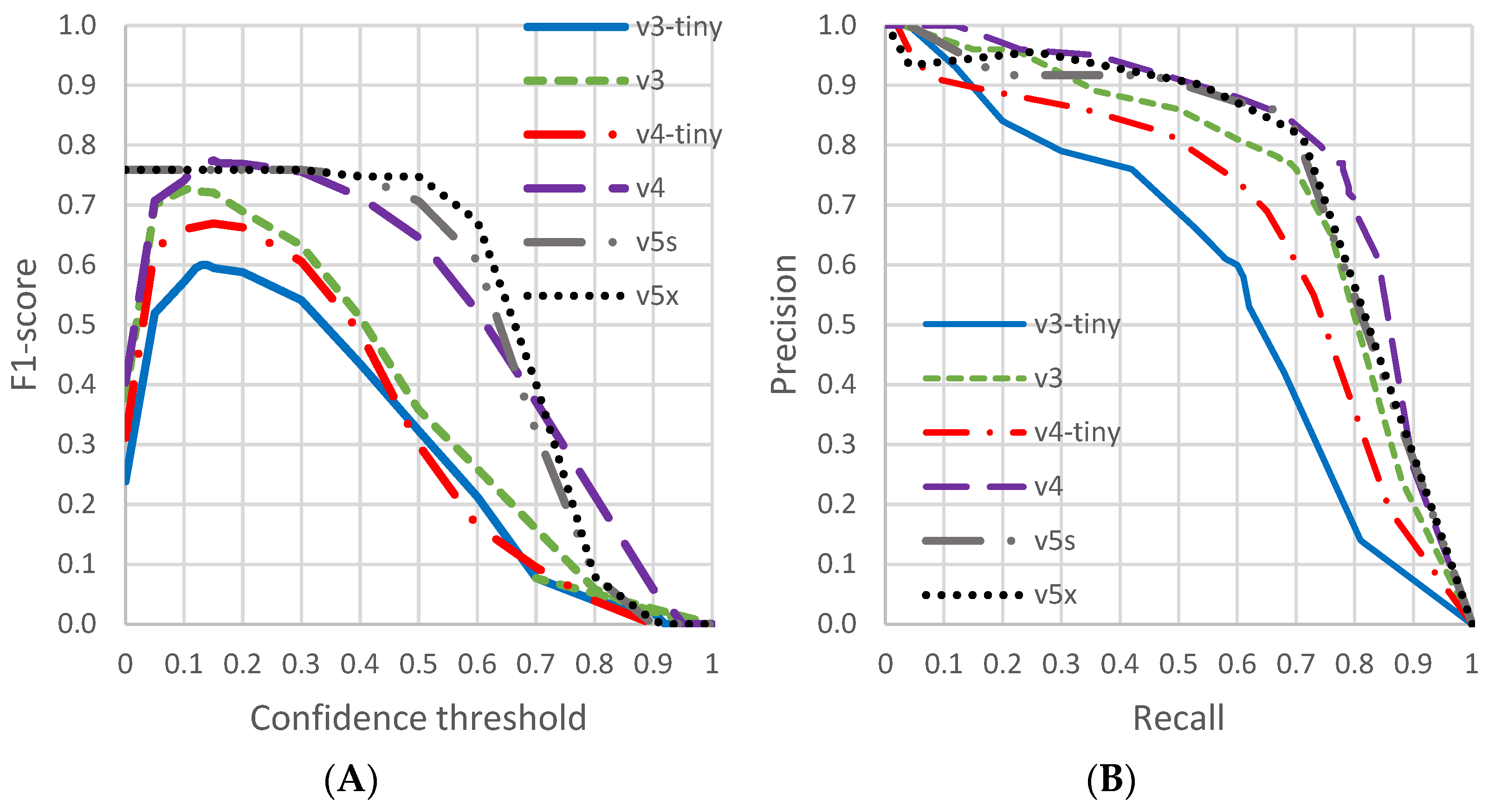
V5x	7.00	70.6%	76.1%	0.77	0.72	0.74

, with the total time that training occurred. Both YOLOv3-tiny and YOLOv4-tiny required about 3.5 h to train for 6000 epochs, while YOLOv3 and YOLOv4 full models required about 15 and 16.5 h, respectively. The training time for YOLOv5-s was 4.66 h, while for YOLOv5-x it was 7 h. The highest value of mAP@50 was reached by YOLOv5x, with 76.1% of the best mAP@50. The tiny models’ best mAP value was achieved by YOLOv5s (73.1%).

During the training, loss and mAP graphs were produced (Figure 1). In YOLOv3-tiny, YOLOv3, YOLOv4, and YOLOv4-tiny loss and mAP reached a stable value after ~1800 epochs (about 30% of the total training). Differently, PyTorch models (YOLOv5) reached a stable value after ~10 epochs, approximately 10% of the total training epochs. The use of a similar training time for all six models would have promoted overfitting of the models.

3.1. Accuracy Assessment on the Validation Dataset

The validation dataset, which was composed of 54 images with the actual number of bunches recorded, was classified using the best bunch detection models previously trained. The comparison was performed in terms of F1 score and mAP@50. Besides, detection speed was evaluated in terms of Frames Per Second (FPS) for each model to study the opportunity to use previously trained models for real-time detection. Metrics calculated on this validation dataset differed from the previously calculated since the validation images were unknown to the trained models.

Figure 2 shows the results of the F-1 score and mAP@50 comparison for objects (bunches) contained in the images dataset. YOLOv5x was characterised by the highest value of mAP@50 and the second-highest value of F1-score. Conversely, YOLOv4 showed the highest value of F1-score and the second-highest value of mAP@50. YOLOv5s model outperformed both the v3-tiny and the v4-tiny, showing metrics similar to full models. Since metrics were extracted from the total number of objects (bunches) in the dataset, it was not possible to perform variance analysis.

The results of the detection time comparison are shown in Figure 3. Detection time was assessed for each image using all the models. One-way ANOVA and Tukey’s multiple comparison tests showed statically significant differences among the models. The average detection speed was ~200, ~196, ~61, ~35, ~31, and ~32 FPS for the v3-tiny, v4-tiny, v5s, v3, v4, and v5x model, respectively.

3.2. Precision–Recall Curves and Best Confident Threshold Definition

The confidence threshold in object detection represents the probability that an estimated bounding box contains an object. In all the analyses performed up to this point, a confidence threshold of 0.25 was used, as it represents the benchmark value for YOLO models [10]. Figure 4A shows the precision–recall curves for each YOLO model. The area under the curve was estimated with the mAP@50. In Figure 4B, confidence thresholds were adjusted to achieve the best F-1 score value for each model. According to this optimisation, the best confidence thresholds were 0.14, 0.12, 0.10, 0.11, 0.15, and 0.10 for the v3-tiny, v4-tiny, v5s, v3, v4, and v5x model, respectively.

3.3. Validation to Estimate Real Numbers of Bunches

The models optimised for the confidence thresholds were finally used to detect the Real Number of Bunches (R_NoB) in validation dataset images, with the actual number of bunches recorded. The bunch occlusion problem was partially overcome by applying a correction coefficient to estimate bunches covered by other vine structures. The estimated number of bunches was then calculated with the formula proposed by Bresilla et al. [40], which is presented in Equation (2). Such a formula allows for the limitation of occlusion and low average precision effects. The percentage of Visible Bunches not covered by other vine structures (%V_NoB) was defined as the Visible Number of Bunches (V_NoB) divided by the R_NoB counted in the field. In the validation populated with images of vines spur cordon-trained, the %V_NoB was 88%.

$${Esimated}_{NOB}=D_{NOB}+[D_{NOB}\ast (1-F_1\left)\right]+\left\{\right(1-\%V_{NOB})\ast [D_{NOB}\ast (1-F_1)\left]\right\}$$

(2)

In Equation (2), D_NoB represents the number of bunches detected by the model, F₁, the F-1 score of the model calculated only for the latter dataset (with counting), and %V_NoB is the percentage of visible bunches on the real number.

Table 4. Average percentage of TP Bunches on R_NoB, F1, RMSE, and MAE for each YOLO version.

	v3-Tiny	v4-Tiny	v5s	v3	v4	v5x
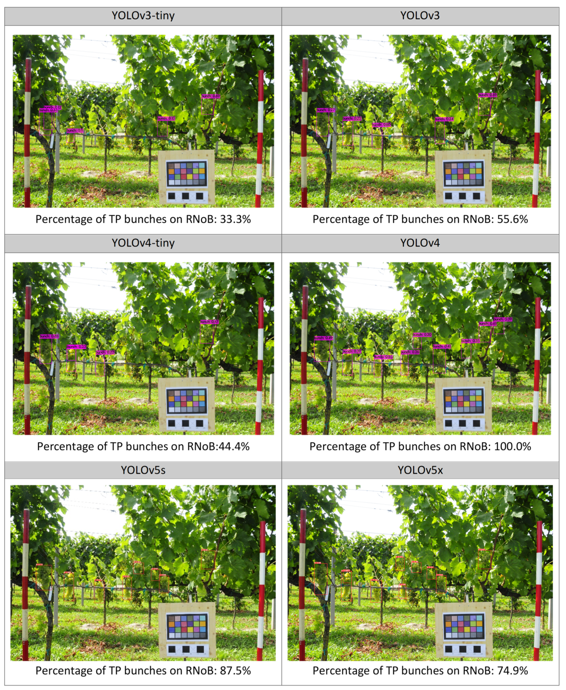
Mean percentage of TP bunches on RNoB	58.0%	70.2%	79.0%	65.3%	78.7%	82.6%
RMSE	3.589	3.236	2.955	2.631	2.931	2.804
MAE	2.739	2.600	1.944	1.919	2.254	2.059

summarises the results of validation on counted images. The mean percentage of TP bunches on R_NoB indicates the number of bunches positively identified on the total, and it was used with the F-1 score to highlight the accuracy of the models to precisely identify bunches. The mean percentage of TP bunches on R_NoB was higher in both v4 models (full and tiny) compared to v3. v4-tiny, and v3 were characterised by the same F-1 score. Estimation errors were calculated in terms of root mean square error (RMSE) and mean absolute error (MAE). An overall higher value of RMSE compared to MAE highlighted the variance of individual errors calculated on every single image. An example of bunch detection and % of True Positive (TP) on R_NoB is shown in Figure 5 and in Appendix A.

4. Discussion

Although the training time was much larger in YOLOv4 compared to other models, YOLOv5x achieved the best values of mAP@50 and F-1 score. Training time was significantly higher in full models (v5x, v4, and v3) rather than tiny models (v5s, v4-tiny, and v3-tiny) due to the higher complexity of the models (expressed in billions of FLOPs in Table 2). The comparison of version 5, 4, and 3 of YOLO within the full and tiny version showed a higher average increment of F-1 in the tiny and “s” versions rather than the full versions (+0.085 and +0.025 for the tiny and full version, respectively). This latter point suggests an exponential increment of complexity in bunch identification. The analysis of loss graphs indicates that training might be stopped before the 6000 and 100 epochs used in this study. Indeed, models reached a stable loss value at ~1800 in the case of YOLOv3, YOLOv3-tiny, YOLOv4-tiny, and YOLOv4. Similarly, YOLOv5 models reached a stable value after ~10 epochs. A reduced training time needed allows optimised training even in the case of a model trained with low-computational power (e.g., training on CPU instead of GPU).

The performance results generated during the training were obtained on the test dataset, which was a part of the same native dataset with the training dataset. To properly validate trained models, the validation dataset (composed of external unknown images) was used. On this dataset, the F-1 score and mAP@50 were higher in v5x and v4 models. The v4-tiny and the v3 full model achieved similar results in terms of F-1, while mAP@50 was higher in the v3 full model. YOLOv5s performed lower than YOLOv4 and YOLOv5x both for mAP@50 and F1-score. F-1 score and mAP@50 were higher on the validation dataset rather than the test dataset because the validation dataset was composed only of field images representing the side of the vine canopy. In contrast, the test dataset was composed even of images acquired out of the vineyard and representing only one bunch at the forefront. In terms of detection time, each model showed that the detection speed allowed the real-time bunch detection on the virtual machine, as it was higher than 30 FPS for all models (Figure 6). YOLOv4-tiny and YOLOv3-tiny showed a detection speed of ~200 FPS, while YOLOv5s reached ~61 FPS and YOLOv3, YOLOv4, and YOLOv5x showed a detection speed of~31 FPS. Such results may be found during an on-field application, taking advantage of cloud computing. Therefore, in the case of portable processing systems with lower computational power, the YOLOv4-tiny model should be preferred. The results of this study confirmed an inverse relationship between detection time and metrics performance. A comparison between YOLOv3, YOLOv4, and YOLOv5 models trained for a different task [58] showed similar results (fastest detection in YOLOv4 and best mAP in YOLOv5); however, a better robustness of YOLOv4 was highlighted. According to Yang et al. [53], YOLOv5 may show the same accuracy as YOLOv4. The study of Lema et al. [59] found the best results in terms of mAP@50 with YOLOv5, without using an unknown external validation dataset.

The optimisation of confidence thresholds on validation highlighted a peak of the F-1 score between 0.1 and 0.2 in all models. However, the v5x, v5s, and v4 model’s confidence threshold curve showed a broader peak of the F-1 score, which was stable in the range of 0.1–0.3 of confidence thresholds. The on-field validation performed comparing the models’ detected number of bunches with the real number of bunches showed higher RMSE and MAE in YOLOv3-tiny and YOLOv4-tiny. Considering the mean percentage of True Positive bunches on the real number of bunches, YOLOv4 reconfirmed a higher performance compared to the YOLOv3 models, while YOLOv5 outperformed other models in all metrics. YOLOv3 showed the worst value of mean percentage of True Positive bunches on the real number of bunches, while both RMSE and MAE were lower than all the other models. This latter situation may be a consequence of the evaluation approach, based only on the number of bunches. A lower accuracy in the YOLOv3 model during the bunch identification caused a higher number of False Positives, which were counted in the total amount of bunches (D_NoB in Equation (2)), sometimes compensating the False Negative. On the other hand, YOLOv5 and YOLOv4 models, which showed higher accuracy, were less affected by this compensation, providing a higher RMSE and MAE even if a higher number of True Positives were detected.

The models developed in this study were trained on white grape varieties, where leaf background and berries are characterised by a similar colour [60]. According to this, the models proposed may be effective in the early stages of the growing season, even in red grape varieties. Nevertheless, the best model developed in this study was YOLOv5x, which was affected by an error of ~2.8 bunches per images, with two vines per image. Considering the average real number of bunches on the validation dataset (10.5 bunches/vines) the average percentage error was 13.3%. The study of Nuske et al. [32] found an average percentage error between 3% and 11%; however, it was based on images acquired during the night with artificial illumination in order to standardise the light conditions. The False Positive–False Negative compensation in bunch counting represents a limitation of the presented object detection models and should be better investigated as well as a correction for occluded bunches [61,62].

Images acquired from a different position may be used in order to achieve better metric performance by using a capture-recapture model [63]. Such models showed to be effective in white grape bunch counting, highlighting a potential application in robotic platforms used and under development for viticulture application. In this latter case, an automated system can be used for yield assessment since the number of bunches showed to be strongly correlated with the spatial variability of yield [62]. In addition, the number of bunches may be converted in yield (fruit load, kg/vines) by using historical bunch weight data.

5. Conclusions

Object detection represents a promising application of deep learning in agriculture, as it can be applied to several issues, such as plant phenotyping, disease identification, and yield estimation. In viticulture, conventional yield estimation is usually based on manual harvesting of sample plants, which is a time-consuming task. The implementation of automatic bunch counting would decrease the time of grape yield estimation. In the current study, four versions of You Only Look Once (YOLO) object detection models were trained and evaluated for real-time bunch detection and counting in white grapes. YOLO models were trained using a heterogeneous dataset populated by images retrieved from open datasets an acquired by the authors. According to the validation results, YOLOv5 and YOLOv4 achieved a higher F-1 score and mAP@50 compared to YOLOv3 models. The validation, based on the real number of bunches, showed that YOLO models were able to detect (True Positive) between 58% and 83% of the real number of bunches of vines. The final estimation, which included a correction for occluded bunches and F-1 score, was affected by a False Positive–False Negative compensation, which decreased the error for YOLOv3 models. According to these considerations, YOLOv5x showed the best performance in terms of correctly detected bunches, while YOLOv4 achieve good results but with a lower detection speed. YOLOv5x was able to estimate the number of bunches per plants with an average error of 13.3%. Although YOLOv5x showed a detection speed that allowed real-time detection, a higher detection speed may be required for on-field application. In this study, the best combination of accuracy and speed was achieved by YOLOv4-tiny. The leaf occlusion and the False Positive–False Negative compensation should be better investigated in order to make the object detection algorithm more effective for viticulture.

References

- Arnó, J.; Casasnovas, J.A.M.; Dasi, M.R.; Rosell, J.R. Review. Precision viticulture. Research topics, challenges and opportunities in site-specific vineyard management. Span. J. Agric. Res. 2009, 7, 779. [Google Scholar] [CrossRef] [Green Version]
- Matese, A.; Di Gennaro, S.F. Technology in precision viticulture: A state of the art review. Int. J. Wine Res. 2015, 7, 69. [Google Scholar] [CrossRef] [Green Version]
- Marinello, F.; Bramley, R.G.V.; Cohen, Y.; Fountas, S.; Guo, H.; Karkee, M.; Martínez-Casasnovas, J.A.; Paraforos, D.S.; Sartori, L.; Sorensen, C.G.; et al. Agriculture and Digital Sustainability: A Digitization Footprint. In Proceedings of the Precision Agriculture ‘21, ECPA 2021, Proceedings of the 13th European Conference on Precision Agriculture, Budapest, Hungary, 18–22 July 2021; Stafford, J.V., Ed.; Wageningen Academic Publishers: Wageningen, The Netherlands, 2019; pp. 83–89. [Google Scholar] [CrossRef]
- Kayad, A.; Sozzi, M.; Gatto, S.; Whelan, B.; Sartori, L.; Marinello, F. Ten years of corn yield dynamics at field scale under digital agriculture solutions: A case study from North Italy. Comput. Electron. Agric. 2021, 185, 106126. [Google Scholar] [CrossRef]
- Seng, K.P.; Ang, L.M.; Schmidtke, L.M.; Rogiers, S.Y. Computer vision and machine learning for viticulture technology. IEEE Access 2018, 6, 67494–67510. [Google Scholar] [CrossRef]
- Liakos, K.G.; Busato, P.; Moshou, D.; Pearson, S.; Bochtis, D. Machine learning in agriculture: A review. Sensors 2018, 18, 2674. [Google Scholar] [CrossRef] [Green Version]
- Kamilaris, A.; Prenafeta-Boldú, F.X. Deep learning in agriculture: A survey. Comput. Electron. Agric. 2018, 147, 70–90. [Google Scholar] [CrossRef] [Green Version]
- Voulodimos, A.; Doulamis, N.; Doulamis, A.; Protopapadakis, E. Deep Learning for Computer Vision: A Brief Review. Comput. Intell. Neurosci. 2018, 2018, 7068349. [Google Scholar] [CrossRef]
- Zhao, Z.Q.; Zheng, P.; Xu, S.T.; Wu, X. Object Detection with Deep Learning: A Review. IEEE Trans. Neural Netw. Learn. Syst. 2019, 30, 3212–3232. [Google Scholar] [CrossRef] [Green Version]
- Redmon, J.; Divvala, S.; Girshick, R.; Farhadi, A. You only look once: Unified, real-time object detection. In Proceedings of the IEEE Conference on Computer Vision and Pattern Recognition (CVPR), Las Vegas, NV, USA, 27–30 June 2016; IEEE Computer Society: Washington, DC, USA, 2016; pp. 779–788. [Google Scholar] [CrossRef] [Green Version]
- Girshick, R.; Donahue, J.; Darrell, T.; Malik, J. Rich feature hierarchies for accurate object detection and semantic segmentation. In Proceedings of the IEEE Conference on Computer Vision and Pattern Recognition (CVPR), Columbus, OH, USA, 23–28 June 2014; IEEE Computer Society: Washington, DC, USA, 2014; pp. 580–587. [Google Scholar] [CrossRef] [Green Version]
- Ren, S.; He, K.; Girshick, R.; Sun, J. Faster R-CNN: Towards Real-Time Object Detection with Region Proposal Networks; IEEE Computer Society: Washington, DC, USA, 2017; Volume 39, pp. 1137–1149. [Google Scholar]
- He, K.; Gkioxari, G.; Dollár, P.; Girshick, R. Mask R-CNN. IEEE Trans. Pattern Anal. Mach. Intell. 2020, 42, 386–397. [Google Scholar] [CrossRef]
- Liu, W.; Anguelov, D.; Erhan, D.; Szegedy, C.; Reed, S.; Fu, C.-Y.Y.; Berg, A.C. SSD: Single Shot MultiBox Detector. In Proceedings of the Computer Vision—ECCV, Amsterdam, The Netherlands, 8–16 October 2016; Leibe, B., Matas, J., Sebe, N., Welling, M., Eds.; Springer International Publishing: Cham, Switzerland, 2016; Volume 9905, pp. 21–37. [Google Scholar]
- Koirala, A.; Walsh, K.B.; Wang, Z.; McCarthy, C. Deep learning—Method overview and review of use for fruit detection and yield estimation. Comput. Electron. Agric. 2019, 162, 219–234. [Google Scholar] [CrossRef]
- Laurent, C.; Oger, B.; Taylor, J.A.; Scholasch, T.; Metay, A.; Tisseyre, B. A review of the issues, methods and perspectives for yield estimation, prediction and forecasting in viticulture. Eur. J. Agron. 2021, 130, 126339. [Google Scholar] [CrossRef]
- Sabbatini, P.; Dami, I.; Howell, G.S. Predicting Harvest Yield in Juice and Wine Grape Vineyards. Mich. State Univ. Ext. 2012, 1–12. [Google Scholar]
- De La Fuente, M.; Linares, R.; Baeza, P.; Miranda, C.; Lissarrague, J.R. Comparison of different methods of grapevine yield prediction in the time window between fruitset and veraison. OENO One 2015, 49, 27–35. [Google Scholar] [CrossRef]
- Coombe, B.G.; McCarthy, M.G. Dynamics of grape berry growth and physiology of ripening. Aust. J. Grape Wine Res. 2000, 6, 131–135. [Google Scholar] [CrossRef]
- Taylor, J.A.; Sanchez, L.; Sams, B.; Haggerty, L.; Jakubowski, R.; Djafour, S.; Bates, T.R. Evaluation of a commercial grape yield monitor for use mid-season and at-harvest. OENO One 2016, 50, 57–63. [Google Scholar] [CrossRef] [Green Version]
- Sozzi, M.; Kayad, A.; Tomasi, D.; Lovat, L.; Marinello, F.; Sartori, L. Assessment of grapevine yield and quality using a canopy spectral index in white grape variety. In Proceedings of the Precision Agriculture ‘19, ECPA 2019, Proceedings of the 12th European Conference on Precision Agriculture, Montpellier, France, 8–11 July 2019; Stafford, J.V., Ed.; Wageningen Academic Publishers: Wageningen, The Netherlands, 2019; pp. 181–186. [Google Scholar] [CrossRef]
- Hall, A. Remote sensing applications for viticultural terroir analysis. Elements 2018, 14, 185–190. [Google Scholar] [CrossRef]
- Cogato, A.; Meggio, F.; Collins, C.; Marinello, F. Medium-Resolution Multispectral Data from Sentinel-2 to Assess the Damage and the Recovery Time of Late Frost on Vineyards. Remote Sens. 2020, 12, 1896. [Google Scholar] [CrossRef]
- Sozzi, M.; Kayad, A.; Giora, D.; Sartori, L.; Marinello, F. Cost-effectiveness and performance of optical satellites constellation for Precision Agriculture. In Proceedings of the Precision Agriculture ‘19, ECPA 2019, Proceedings of the 12th European Conference on Precision Agriculture, Montpellier, France, 8–11 July 2019; Stafford, J.V., Ed.; Wageningen Academic Publishers: Wageningen, The Netherlands, 2019; pp. 501–507. [Google Scholar] [CrossRef]
- Sozzi, M.; Kayad, A.; Gobbo, S.; Cogato, A.; Sartori, L.; Marinello, F.; Singh, V.; Huang, Y. Economic Comparison of Satellite, Plane and UAV-Acquired NDVI Images for Site-Specific Nitrogen Application: Observations from Italy. Agronomy 2021, 11, 2098. [Google Scholar] [CrossRef]
- Cogato, A.; Wu, L.; Jewan, S.Y.Y.; Meggio, F.; Marinello, F.; Sozzi, M.; Pagay, V. Evaluating the Spectral and Physiological Responses of Grapevines (Vitis vinifera L.) to Heat and Water Stresses under Different Vineyard Cooling and Irrigation Strategies. Agronomy 2021, 11, 1940. [Google Scholar] [CrossRef]
- Bramley, R.G.V.; Le Moigne, M.; Evain, S.; Ouzman, J.; Florin, L.; Fadaili, E.M.; Hinze, C.J.; Cerovic, Z.G. On-the-go sensing of grape berry anthocyanins during commercial harvest: Development and prospects. Aust. J. Grape Wine Res. 2011, 17, 316–326. [Google Scholar] [CrossRef]
- Henry, D.; Aubert, H.; Veronese, T. Proximal Radar Sensors for Precision Viticulture. IEEE Trans. Geosci. Remote Sens. 2019, 57, 4624–4635. [Google Scholar] [CrossRef]
- Gongal, A.; Amatya, S.; Karkee, M.; Zhang, Q.; Lewis, K. Sensors and systems for fruit detection and localization: A review. Comput. Electron. Agric. 2015, 116, 8–19. [Google Scholar] [CrossRef]
- Aquino, A.; Millan, B.; Diago, M.P.; Tardaguila, J. Automated early yield prediction in vineyards from on-the-go image acquisition. Comput. Electron. Agric. 2018, 144, 26–36. [Google Scholar] [CrossRef]
- Nuske, S.; Achar, S.; Bates, T.; Narasimhan, S.; Singh, S. Yield estimation in vineyards by visual grape detection. In Proceedings of the 2011 IEEE/RSJ International Conference on Intelligent Robots and Systems, San Francisco, CA, USA, 25–30 September 2011; IEEE: Manhattan, NY, USA, 2011; pp. 2352–2358. [Google Scholar]
- Nuske, S.; Wilshusen, K.; Achar, S.; Yoder, L.; Singh, S. Automated visual yield estimation in vineyards. J. Field Robot. 2014, 31, 837–860. [Google Scholar] [CrossRef]
- Di Gennaro, S.F.; Toscano, P.; Cinat, P.; Berton, A.; Matese, A. A precision viticulture UAV-based approach for early yield prediction in vineyard. In Proceedings of the Precision Agriculture ‘19, ECPA 2019, Proceedings of the 12th European Conference on Precision Agriculture, Montpellier, France, 8–11 July 2019; Stafford, J.V., Ed.; Wageningen Academic Publishers: Wageningen, The Netherlands, 2019; pp. 373–379. [Google Scholar] [CrossRef]
- Comba, L.; Biglia, A.; Aimonino, D.R.; Gay, P. Unsupervised detection of vineyards by 3D point-cloud UAV photogrammetry for precision agriculture. Comput. Electron. Agric. 2018, 155, 84–95. [Google Scholar] [CrossRef]
- Santos, T.T.; de Souza, L.L.; dos Santos, A.A.; Avila, S. Grape detection, segmentation, and tracking using deep neural networks and three-dimensional association. Comput. Electron. Agric. 2020, 170, 105247. [Google Scholar] [CrossRef] [Green Version]
- Redmon, J.; Farhadi, A. YOLOv3: An Incremental Improvement. arXiv 2018, arXiv:1804.02767. [Google Scholar]
- Zhang, Y.; Shen, Y.; Zhang, J. An improved tiny-yolov3 pedestrian detection algorithm. Optik 2019, 183, 17–23. [Google Scholar] [CrossRef]
- Hendry; Chen, R.C. Automatic License Plate Recognition via sliding-window darknet-YOLO deep learning. Image Vis. Comput. 2019, 87, 47–56. [Google Scholar] [CrossRef]
- Zhou, J.; Jing, J.; Zhang, H.; Zhen, W.; Wang, Z.; Huang, H. Real-time fabric defect detection algorithm based on s-yolov3 model. Laser Optoelectron. Prog. 2020, 57, 161001. [Google Scholar] [CrossRef]
- Bresilla, K.; Perulli, G.D.; Boini, A.; Morandi, B.; Grappadelli, L.C.; Manfrini, L. Single-Shot Convolution Neural Networks for Real-Time Fruit Detection Within the Tree. Front. Plant Sci. 2019, 10, 611. [Google Scholar] [CrossRef] [PubMed] [Green Version]
- Tian, Y.; Yang, G.; Wang, Z.; Wang, H.; Li, E.; Liang, Z. Apple detection during different growth stages in orchards using the improved YOLO-V3 model. Comput. Electron. Agric. 2019, 157, 417–426. [Google Scholar] [CrossRef]
- Li, X.; Qin, Y.; Wang, F.; Guo, F.; Yeow, J.T.W. Pitaya detection in orchards using the MobileNet-YOLO model. In Proceedings of the Chinese Control Conference, CCC, Shenyang, China, 27–30 July 2020; IEEE Computer Society: Washington, DC, USA, 2020; Volume 2020, pp. 6274–6278. [Google Scholar]
- Morbekar, A.; Parihar, A.; Jadhav, R. Crop disease detection using YOLO. In Proceedings of the 2020 International Conference for Emerging Technology, INCET 2020, Belgaum, India, 5–7 June 2020; Institute of Electrical and Electronics Engineers Inc.: Piscataway, NJ, USA, 2020. [Google Scholar]
- Ponnusamy, V.; Coumaran, A.; Shunmugam, A.S.; Rajaram, K.; Senthilvelavan, S. Smart Glass: Real-Time Leaf Disease Detection using YOLO Transfer Learning. In Proceedings of the 2020 IEEE International Conference on Communication and Signal Processing, ICCSP 2020, Chennai, India, 28–30 July 2020; Institute of Electrical and Electronics Engineers Inc.: Piscataway, NJ, USA, 2020; pp. 1150–1154. [Google Scholar]
- Zhong, Y.; Gao, J.; Lei, Q.; Zhou, Y. A Vision-Based Counting and Recognition System for Flying Insects in Intelligent Agriculture. Sensors 2018, 18, 1489. [Google Scholar] [CrossRef] [PubMed] [Green Version]
- Abdulsalam, M.; Aouf, N. Deep Weed Detector/Classifier Network for Precision Agriculture; Institute of Electrical and Electronics Engineers (IEEE): Piscataway, NJ, USA, 2020; pp. 1087–1092. [Google Scholar]
- Yin, Y.; Li, H.; Fu, W. Faster-YOLO: An accurate and faster object detection method. Digit. Signal Process. 2020, 102, 102756. [Google Scholar] [CrossRef]
- Wang, C.Y.; Liao, H.Y.M.; Wu, Y.H.; Chen, P.Y.; Hsieh, J.W.; Yeh, I.H. CSPNet: A new backbone that can enhance learning capability of CNN. In Proceedings of the IEEE Conference on Computer Vision and Pattern Recognition (CVPR), Seattle, WA, USA, 16–18 June 2020; IEEE Computer Society: Washington, DC, USA, 2020; Volume 2020, pp. 1571–1580. [Google Scholar]
- Bochkovskiy, A.; Wang, C.-Y.; Liao, H.-Y.M. YOLOv4: Optimal Speed and Accuracy of Object Detection. arXiv 2020, arXiv:2004.10934. [Google Scholar]
- Zheng, Z.; Wang, P.; Liu, W.; Li, J.; Ye, R.; Ren, D. Distance-IoU Loss: Faster and Better Learning for Bounding Box Regression. In Proceedings of the AAAI Conference on Artificial Intelligence, Phoenix, AZ, USA, 12–17 February 2016. [Google Scholar]
- Jocher, G.; Stoken, A.; Borovec, J.; Christopher, S.T.A.N.; Laughing, L.C. ultralytics/yolov5: v4.0-nn.SiLU() activations, Weights & Biases logging, PyTorch Hub integration. Zenodo 2021. [Google Scholar] [CrossRef]
- Iyer, R.; Shashikant Ringe, P.; Varadharajan Iyer, R.; Prabhulal Bhensdadiya, K. Comparison of YOLOv3, YOLOv5s and MobileNet-SSD V2 for Real-Time Mask Detection. Artic. Int. J. Res. Eng. Technol. 2021, 8, 1156–1160. [Google Scholar]
- Yang, G.; Feng, W.; Jin, J.; Lei, Q.; Li, X.; Gui, G.; Wang, W. Face Mask Recognition System with YOLOV5 Based on Image Recognition. In Proceedings of the 2020 IEEE 6th International Conference on Computer and Communications (ICCC), Chengdu, China, 11–14 December 2020; Volume 1, pp. 1398–1404. [Google Scholar] [CrossRef]
- Chetlur, S.; Woolley, C.; Vandermersch, P.; Cohen, J.; Tran, J.; Catanzaro, B.; Shelhamer, E. cuDNN: Efficient Primitives for Deep Learning. arXiv 2014, arXiv:1410.0759. [Google Scholar]
- Kuznetsova, A.; Rom, H.; Alldrin, N.; Uijlings, J.; Krasin, I.; Pont-Tuset, J.; Kamali, S.; Popov, S.; Malloci, M.; Kolesnikov, A.; et al. The Open Images Dataset V4: Unified Image Classification, Object Detection, and Visual Relationship Detection at Scale. Int. J. Comput. Vis. 2020, 128, 1956–1981. [Google Scholar] [CrossRef] [Green Version]
- Kwon, Y.; Choi, W.; Marrable, D.; Abdulatipov, R.; Loïck, J. Yolo_label 2020. Available online: https://github.com/developer0hye/Yolo_Label (accessed on 23 January 2022).
- Dice, L.R. Measures of the Amount of Ecologic Association between Species. Ecology 1945, 26, 297–302. [Google Scholar] [CrossRef]
- Li, S.; Gu, X.; Xu, X.; Xu, D.; Zhang, T.; Liu, Z.; Dong, Q. Detection of concealed cracks from ground penetrating radar images based on deep learning algorithm. Constr. Build. Mater. 2021, 273, 121949. [Google Scholar] [CrossRef]
- Lema, D.G.; Pedrayes, O.D.; Usamentiaga, R.; García, D.F.; Alonso, Á. Cost-performance evaluation of a recognition service of livestock activity using aerial images. Remote Sens. 2021, 13, 2318. [Google Scholar] [CrossRef]
- Aguiar, A.S.; Magalhães, S.A.; Dos Santos, F.N.; Castro, L.; Pinho, T.; Valente, J.; Martins, R.; Boaventura-Cunha, J. Grape Bunch Detection at Different Growth Stages Using Deep Learning Quantized Models. Agronomy 2021, 11, 1890. [Google Scholar] [CrossRef]
- Taylor, J.A.; Dresser, J.L.; Hickey, C.C.; Nuske, S.T.; Bates, T.R. Considerations on spatial crop load mapping. Aust. J. Grape Wine Res. 2019, 25, 144–155. [Google Scholar] [CrossRef]
- Sozzi, M.; Cantalamessa, S.; Cogato, A.; Kayad, A.; Marinello, F. Grape Yield Spatial Variability Assessment Using YOLOv4 Object Detection Algorithm. In Proceedings of the Precision Agriculture ‘21, ECPA 2021, Proceedings of the 13th European Conference on Precision Agriculture, Budapest, Hungary, 18–22 July 2021; Stafford, J.V., Ed.; Wageningen Academic Publishers: Wageningen, The Netherlands, 2019; pp. 193–198. [Google Scholar] [CrossRef]
- Pollock, K.H. A Capture-Recapture Design Robust to Unequal Probability of Capture. J. Wildl. Manag. 1982, 46, 752. [Google Scholar] [CrossRef]