In-Season Prediction of Corn Grain Yield through PlanetScope and Sentinel-2 Images

Abstract

Crop growth and yield monitoring are essential for food security and agricultural economic return prediction. Remote sensing is an efficient technique for measuring growing season crop canopies and providing information on the spatial variability of crop yields. In this study, ten vegetation indices (VIs) derived from time series PlanetScope and Sentinel-2 images were used to investigate the potential to estimate corn grain yield with different regression methods. A field-scale spatial crop yield prediction model was developed and used to produce yield maps depicting spatial variability in the field. Results from this study clearly showed that high-resolution PlanetScope satellite data could be used to detect the corn yield variability at field level, which could explain 15% more variability than Sentinel-2A data at the same spatial resolution of 10 m. Comparison of the model performance and variable importance measure between models illustrated satisfactory results for assessing corn productivity with VIs. The green chlorophyll vegetation index (GCVI) values consistently produced the highest correlations with corn yield, accounting for 72% of the observed spatial variation in corn yield. More reliable quantitative yield estimation could be made using a multi-linear stepwise regression (MSR) method with multiple VIs. Good agreement between observed and predicted yield was achieved with the coefficient of determination value being 0.81 at 86 days after seeding. The results would help farmers and decision-makers generate predicted yield maps, identify crop yield variability, and make further crop management practices timely.

1. Introduction

Monitoring and predicting crop phenology, growth, and yield is an important component of global food security and plays a key role in domestic and global markets, policies, and decision-making [1,2]. Yield is commonly measured using manual sampling and ground-based visits, which are extremely time and labor-consuming, and difficult to provide information on the spatial variability of crop yield [3]. Due to the lack of a large amount of input data on management practices, such as variety, sowing date, seed rate, fertilization schedule, irrigation, etc., it is difficult to use crop growth models to monitor crop growth and estimate yield at regional scales [4,5,6]. However, rapid and effective acquisition of crop yield information, accurate forecast of crop productivity, and understanding of yield variability at a regional scale are critical to farm management and decision making [7].

Compared to crop growth models, remote sensing (RS) technology provides real-time and large-area data collection capabilities at a range of spatial scales, which has already been used to produce numerous agriculture-related parameters [8,9,10]. Crop yield estimation has been emphasized as a critical component of RS applications in agricultural studies. There have been many attempts in the applications of RS to estimate the final yields for wheat (Triticum aestivum L.) [9,11,12], barley (Hordeum vulgare. L) [13,14], maize (Zea mays L.) [15,16], rice (Oryza sativa L.) [10,17,18], potato (Solanum tuberosum L.) [19], cotton (Gossypium L.) [20,21,22], and a variety of fruits [23,24,25]. All the studies indicated that RS technology was prospective and promising in regional crop yield estimation, monitoring, and mapping.

Satellite-based RS techniques can obtain satisfactory images at local and regional scales. Advanced very high resolution radiometer (AVHRR) and Moderate-resolution imaging spectroradiometer (MODIS) data with coarse spatial-resolutions have been repeatedly adapted to estimate crop yields at the global and national levels [2,26,27,28]. Remote sensing data with medium spatial-resolution provides a guarantee for dynamic monitoring of crop growth and yield estimation at county-scale with time-efficient surface observations [28,29,30]. Such as, Landsat 8 (30 m)and coarse spatial-resolution (1/3 km) PROBA-V images were used together to extract temporal characteristics of alfalfa farms and model alfalfa yield in the Moghan Plain, Iran [12]. Nevertheless, an accurate crop yield estimation with sufficient lead time at field scale is more important for farmers in crop management, resource mobilization, agri-commodity trading, and crop insurance [6,9]. More often than not, estimating crop yield at the field level has been laborious and complex due to the difficulty of obtaining actual crop yield data in the field and RS data with high spatiotemporal and spectral resolution [6,12,31,32]. Skakun’s research showed that moving to coarser resolution data of 10 m, 20 m, and 30 m reduced the explained yield variability to 86%, 72%, and 59%, respectively [33]. In recent years, Sentinel-2 satellite imagery has been successfully used to model crop grain yield at field and within-field scales due to its spectral bands (visible and near infrared (NIR), red-edge (RE), and short-wave infrared bands), spatial resolutions (10 m, 20 m and 20 m), and open accessibility [3,7,11,34,35]. Hunt et al. demonstrated accurate verification of within-field variability and relatively high accuracy of yield estimation and mapping at 10 m resolution using Sentinel-2 data (RMSE 0.66 t/ha) [7]. The increased spatial resolution of satellites provides more granular data for accurate monitoring of crop status and enables high-precision yield estimation at field and within-field scales. Recent years, PlanetScope images with spatial resolution of 3 m provide more detailed surface information in the visible and NIR bands, and have been shown to outperform in precision agriculture research [36,37]. Skakun et al. showed that 100% of the within-field corn and soybean yield variability could be explained with a 3 m image (PlanetScope satellite), which was 14% higher than Sentinel-2 (10 m) [33]. On the one hand, the performance of PlanetScope data in yield estimation needs to be verified. On the other hand, It is still a challenge to accurately predict yield well ahead of harvest at field and within-field scales with minimal field input data [6,38,39].

The photosynthesis of green plants is the essence of crop yield. The crop physiological factors, such as chlorophyll concentration, leaf area index, the ground biomass, etc., influence the crop yield potential, which is defined as the maximum attainable yield per unit land area that can be achieved without stress factors [40]. Spectral information in different RS bands, especially optical bands, is optimized for the calculation of relevant VIs, which are proved to be sensitive to crop physiological parameters and commonly used to predict crop yields [9,12,41]. Studies have shown that early season VIs have significant correlations with corn yields [8,42]. Nevertheless, VIs performed differently in crop yield estimation. While the enhanced vegetation index (EVI) was believed the best predictor for the Corn Belt [1]. Shanahan et al. suggested that the green normalized difference vegetation index (GNDVI) had greater potential to estimate final corn grain yields than the normalized difference vegetation index (NDVI) and transformed soil-adjusted vegetation index (TSAVI) [43]. The perpendicular vegetation index (PVI) provided better average prediction accuracy than NDVI, green vegetation index (GVI), and soil adjusted vegetation index (SAVI) in the corn crop yield prediction studied by Panda et al. [44]. Liaqat et al. found SAVI was better associated with wheat yields when compared to modified soil adjusted vegetation index (MSAVI), NDVI, and EVI [9]. The wide dynamic range vegetation index (WDRVI) demonstrated the highest correlation with county-level statistical corn yields [28]. The sensitivity of VIs to yield estimation remains to be verified.

Empirical methods based on statistical regression between RS derived variables and crop yield are the most commonly used approaches [11]. The availability of many indices has led to multiple VIs being chosen and combined with statistical models for more accurate crop yield estimation [9,45,46]. Recent years have witnessed an emergence of machine learning (ML) regression models to develop an empirical relationship between crop yield and crop canopy features, such as random forest regression (RFR) [7,28] because of their ability to autonomously solve large non-linear problems using datasets from multiple sources [46].

In this study, actual field-level harvester corn grain yield data, as well as time-series images from the PlanetScope and Sentinel-2 A satellites, were obtained to develop VIs-based corn yield estimation models by the comparison of unary linear regression (ULR), stepwise multiple linear regression (SMLR) and RFR ML methods. The main purposes of this research were to investigate the sensitivity of VIs derived from high spatial-resolution images to corn yield prediction, to explore the ability of PlanetScope data to estimate within-field corn yield variability in comparison to the results with Sentinel-2 data, and to understand the optimal growth period for corn yield estimation.

2. Materials and Methods

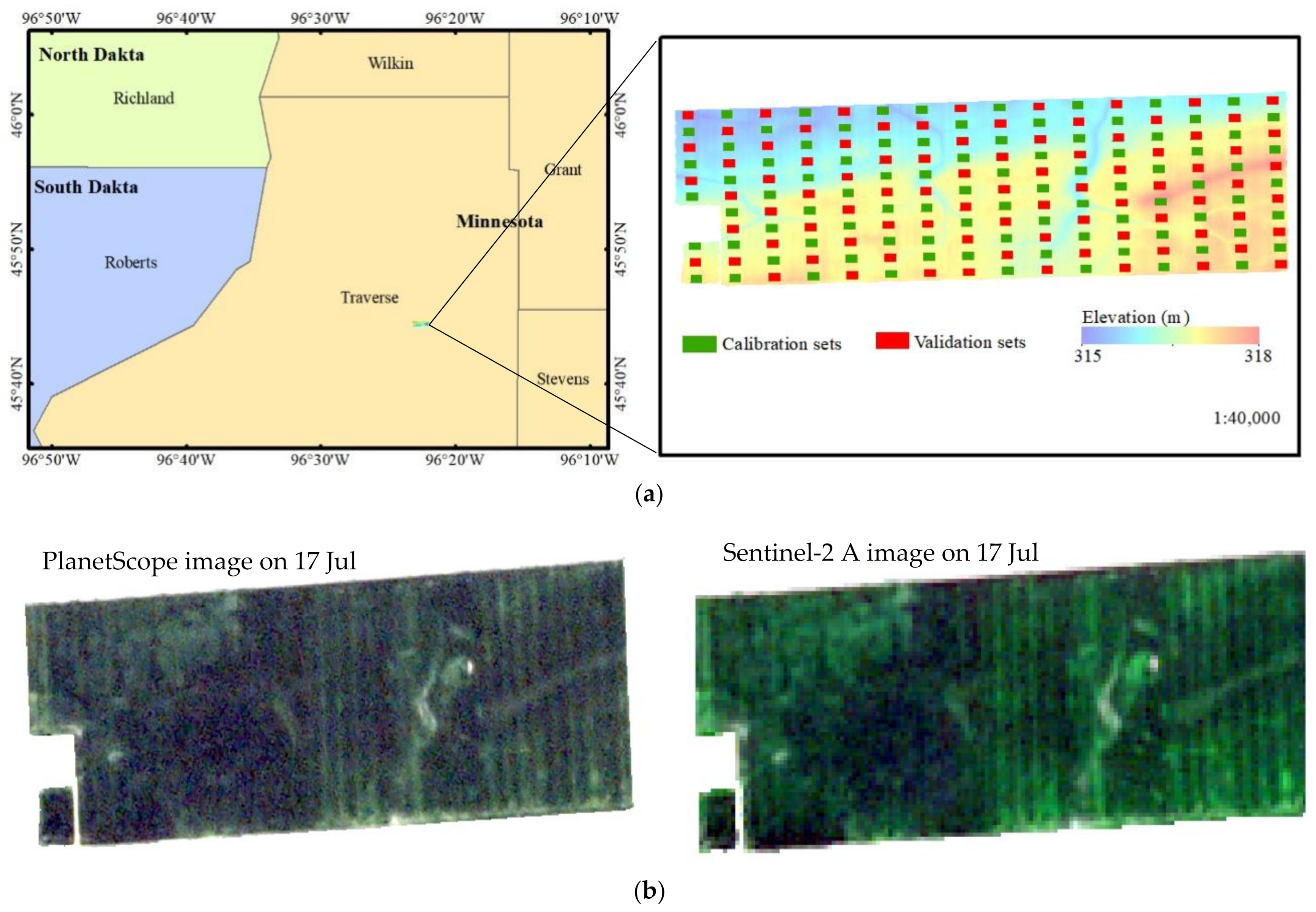
2.1. Field Site and Grain Yield Acquisition

The corn field was located in Wheaton, Minnesota (MN), USA (96.37E, 45.74N), which comprised an area of approximately 100 ha (Figure 1). The farming in this region is characterized by one harvest per year, with corn being the prevalent crop. Generally, the corn crop is typically planted in early to late May and harvested between late September to early October. The normal annual precipitation in this region ranges from 455 to 635 mm, and a mean annual temperature of 1.7 to 5.0 °C [47]. Soils in this region are primarily developed in lacustrine parent material with poor drainage, and the dominant type was silty clay loam soil. Less topographic relief was observed in this field with slope variations of less than 1%. The corn hybrid 76S92 VT2PRO widely adapted to different environments was cultivated in this study. It has an excellent vigor early in the season, strong stress tolerance, very good late season standability, and consistent yielding with fast dry down. Urea fertilizer was spread prior to planting corn on 6 May 2018. In-season topdressing was applied with 28% urea ammonium nitrate solution and a Y-DROP system after corn canopy closure on 26 June 2018. This year was a normal year without extreme weather. Agronomic management practices were conventional for row crop agriculture in this region of the USA. By the end of the crop season, the field was harvested with a GPS-referenced 8-row John Deere rotor combine harvester equipped with optical yield monitors. The combine monitor was calibrated using the same corn hybrid. The yield was determined as the grain biomass collected during harvest and recorded in megagram per hectare (Mg·ha⁻¹) on a standard moisture basis of 15.5%. Due to the cutting width of 6 m of the combine harvester used in this field, and the the furthest distance of 6 m for the yield points, all the yield points were resampled to 10 m resolution using the inverse distance weighting (IDW) spatial interpolation method.

2.2. Satellite Data Collection and Preprocessing

2.2.1. PlanetScope Image Processing

A total of eight PlanetScope surface reflectance (SR) image products (Level 3B) were collected during the corn growing season from June to middle August. All the images were orthorectified, atmospherically corrected using the 6SV2.1 radiative transfer code, scaled, and delivered as analytic 4-band products [48]. PlanetScope satellite imagery has 4 multi-spectral bands including blue (455–515 nm), green (500–590 nm), red (590–670 nm), and NIR (780–860 nm) with a 3 m resolution. All the bands were resampled to 10 m resolution to match that of Sentinel-2 data.

2.2.2. Sentinel-2A Image Processing

Six cloud-free Sentinel-2A images (Level 1C) were downloaded from the European Space Agency (ESA) website (https://scihub.copernicus.eu/dhus/#/home, accessed on 1 March 2020). Radiometric calibration and atmospheric correction were performed in the Sen2Cor processor released by ESA. The corrected data were resampled to 10 m in the SNAP processor using the nearest neighbor interpolation method. To be consistent with PlanetScope data, the blue (458–523 nm), green (543–578 nm), red (650–680 nm), and NIR (785–900 nm) bands were used to extract VIs. Details of the satellite images used in this study are shown in

Table 1. Satellite images collected during the corn growing season in 2018.

Image	Acquisition Date	Days after Seeding (DAS)	Growth Stage	Product Level
PlanetScope	3 Jun., 18 Jun., 5 Jul., 17 Jul.	29, 44, 61, 73	V6, V10, V17, VT	Level 3B
	23 Jul., 30 Jul., 8 Aug., 15 Aug.	79, 86, 95, 102	R1, R2, R3, R4
Sentinel-2A	7 Jul., 17 Jul. 22 Jul., 27 Jul., 6 Aug., 11 Aug.	63, 73 78, 83, 93, 98	V17, VT R1, R2, R3, R3	Level 1C

. All the images were projected to a cartographic projection (WGS84-UTM).

2.3. Vegetation Indices

Numerous VIs have been developed and widely applied in cropland cover changes, vegetation classification, environmental change detection, crop detection, and yield estimation. In this study, ten commonly used VIs related to vegetation growth and biomass were calculated from PlanetScope and Sentinel-2A images to evaluate variation in yield, including SR, MSR, NDVI, GNDVI, SAVI, EVI2, MCARI2, MSAVI, WDRVI, and GCVI (see

Table 2. VIs calculated using satellite imagery, where R is the reflectance of each band.

Vegetation Index	Equation	References
SR (Simple Ratio)	${\mathrm{R}}_{\mathrm{NIR}}/{\mathrm{R}}_{\mathrm{red}}$	[49]
MSR (Modified Simple Ratio)	$\left({\mathrm{R}}_{\mathrm{NIR}}/{\mathrm{R}}_{\mathrm{red}}-1\right)/\mathrm{Sqrt}\left({\mathrm{R}}_{\mathrm{NIR}}/{\mathrm{R}}_{\mathrm{red}}+1\right)$	[50]
NDVI (Normalized Differenced Vegetation Index)	$({\mathrm{R}}_{\mathrm{NIR}}-{\mathrm{R}}_{\mathrm{red}})/\left({\mathrm{R}}_{\mathrm{NIR}}+{\mathrm{R}}_{\mathrm{red}}\right)$	[51]
GNDVI (Green Normalized Differenced Vegetation Index)	$({\mathrm{R}}_{\mathrm{NIR}}-{\mathrm{R}}_{\mathrm{green}})/\left({\mathrm{R}}_{\mathrm{NIR}}+{\mathrm{R}}_{\mathrm{green}}\right)$	[52]
SAVI (Optimized Soil-Adjusted Vegetation Index)	$1.5({\mathrm{R}}_{\mathrm{NIR}}-{\mathrm{R}}_{\mathrm{red}})/\left({\mathrm{R}}_{\mathrm{NIR}}+{\mathrm{R}}_{\mathrm{red}}+0.5\right)$	[53]
EVI2 (Enhanced Vegetation Index)	$2.5({\mathrm{R}}_{\mathrm{NIR}}-{\mathrm{R}}_{\mathrm{red}})/\left({\mathrm{R}}_{\mathrm{NIR}}+2.4{\ast \mathrm{R}}_{\mathrm{red}}+1\right)$	[54]
MCARI2 (Modified chlorophyll absorption reflectivity index)	$\frac{1.5\left[2.5({\mathrm{R}}_{\mathrm{NIR}}-{\mathrm{R}}_{\mathrm{red}}\right)-1.3\left({\mathrm{R}}_{\mathrm{NIR}}-{\mathrm{R}}_{\mathrm{green}}\right)]}{\sqrt{{\left(2{\mathrm{R}}_{\mathrm{NIR}}+1\right)}^2-\left(6{\mathrm{R}}_{\mathrm{NIR}}-5\sqrt{{\mathrm{R}}_{\mathrm{red}}}\right)}-0.5}$	[55]
MSAVI (Modified soil-adjusted vegetation index)	$$\begin{gathered} 0.5\left[2{\mathrm{R}}_{\mathrm{NIR}}+1 \\ -\sqrt{{\left(2{\mathrm{R}}_{\mathrm{NIR}}+1\right)}^2-8\left({\mathrm{R}}_{\mathrm{NIR}}-{\mathrm{R}}_{\mathrm{red}}\right)}\right] \end{gathered}$$	[56]
WDRVI (Wide dynamic range vegetation index)	$\left(0.2{\mathrm{R}}_{\mathrm{NIR}}-{\mathrm{R}}_{\mathrm{red}}\right)/\left(0.2{\mathrm{R}}_{\mathrm{NIR}}+{\mathrm{R}}_{\mathrm{red}}\right)$	[57]
GCVI (Green chlorophyll vegetation index)	${\mathrm{R}}_{\mathrm{NIR}}/{\mathrm{R}}_{\mathrm{green}}-1$	[58]

for expressions).

2.4. Data Analysis

Based on the ten VIs, ULR and SMLR were adopted to establish the corn yield estimation equations in a linear relationship. In SMLR, the best yield model at each growth stage was chosen according to the Akaike Information Criterion (AIC), which was computed with the stepAIC function from the MASS library in R Studio [59].

RFR algorithms have been widely employed to relate remotely sensed data to crop physicochemical parameters [7,28]. It is one of the representatives of ensemble learning algorithms that integrate many decision trees and outputs results by voting. A group of decision trees are independently trained in regression problems, and their predictions are averaged as the final output [60]. In this study, a RFR algorithm was performed to test the utility of the generated VIs in predicting corn yield in a nonlinear regression model. The optimal random forest model was built using the 5-fold GridSearchCV method in the Scikit-learn library in Python 3.8. The algorithm uses each set of hyperparameters to train the model within the specified parameter range and selects the combination of hyperparameters with the minimum error of the verification set. The approximate range of the optimal parameters for RFR model was obtained through repeated attempts, and then the optimal solution was specified under the small range for the obtained results. The number of decision trees in the study was set to 2, 3, 4, 5, 6, 7, 8, 9, 10, 12, 15, 20, 30, 50, 100, 150 and 200, respectively. The randomly selected feature numbers of each decision tree were set to 60%, 70%, 80% and 100% of the total feature numbers, respectively. The maximum tree depth was set to 3, 5, 7, 9, 10, 15 and 20, respectively. In addition, RFR enables feature screening, in which the importance of a variable in estimating crop yield can also be evaluated, indicating the contribution of this feature to model construction.

2.5. Calibration and Validation Datasets

A total of 174 equally spaced sample points in the corn field were selected to extract yield data from the IDW-interpolated yield maps and the VI values from PlanetScope and Sentinel-2 images. It was cross divided into 87 calibration sets and 87 validation sets (Figure 1). The coefficient of determination (R²) and root mean square error (RMSE) of measured and predicted yields in the validation sets were used to evaluate model performance to validate the accuracy and robustness of the derived yield estimation models.

3. Results

3.1. Description of the Yield Data

The raw yield data outside the field mean ±3 sd were cleaned to remove inaccurate grain yield measurements. The cleaned corn yield data of 64,803 yield points were measured and resampled to 10 m resolution using the inverse distance weighting (IDW) spatial interpolation method. IDW-interpolated yield showed a minimum yield of 3.82 Mg·ha⁻¹ and a maximum yield of 15.90 Mg·ha⁻¹ in this field. The mean corn yield in this field was 12.33 Mg·ha⁻¹ and the standard deviation was 2.03 Mg·ha⁻¹.

3.2. Correlation between Yield and Environment Variables

It is generally considered that environmental factors have a certain degree of influence on the formation of yield, and are potential factors affecting spatial distribution of yield. At within field level, the spatial variation of weather is relatively uniform. Topographical features, such as altitude, slope, and aspect have certain impacts on grain yield, especially at the regional scale [11]. Most of the study area is fairly flat, with an altitude difference of less than 3 m. In total, 76.3% of the area had a slope of less than 1 degree (Figure 1). The correlation coefficients between corn yield with altitude, slope, and aspect did not pass the significance test (p > 0.01), indicating that topographical features were unsuitable to be used as influencing factors in crop yield estimation in this study. Under 150 randomly generated points in each soil textures, the ANOVA analysis revealed no significant difference in corn yield among clay loam, Loam, Sandy loam, silt loam, and silty clay loam soil types.

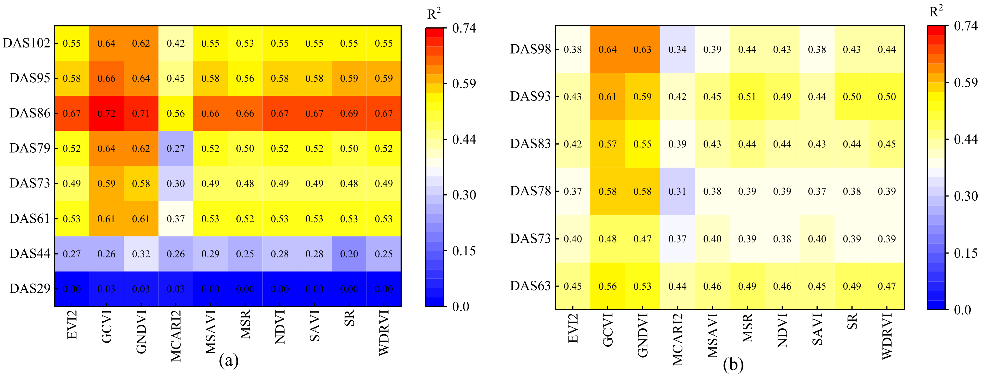
3.3. Correlation between Yield and Vegetation Index

Correlation analysis was conducted between corn yield and VIs in each growth period based on PlanetScope images and Sentinel images, respectively (Figure 2). All the VIs were significantly and positively correlated with corn yield (p < 0.01) except for the stage DAS29. As the corn growth period progressed, the correlation between PlanetScope-based VIs and yield increased first and then decreased (Figure 2a). The inflection point appeared on DAS86. The Coefficient of determination (R²) ranged from 0.56 (MCARI2) to 0.72 (GCVI) on DAS86. Figure 2b shows a similar correlation trend with Sentinel images. All the highest correlations appeared on DAS93 except for GCVI (0.64) and GNDVI (0.63) on DAS98. The R² ranged from 0.42 (MCARI2) to 0.61 (GCVI) on DAS93. The correlation analysis demonstrated that GCVI and GNDVI outperformed other VIs in corn yield prediction.

3.4. Yield Estimation and Validation

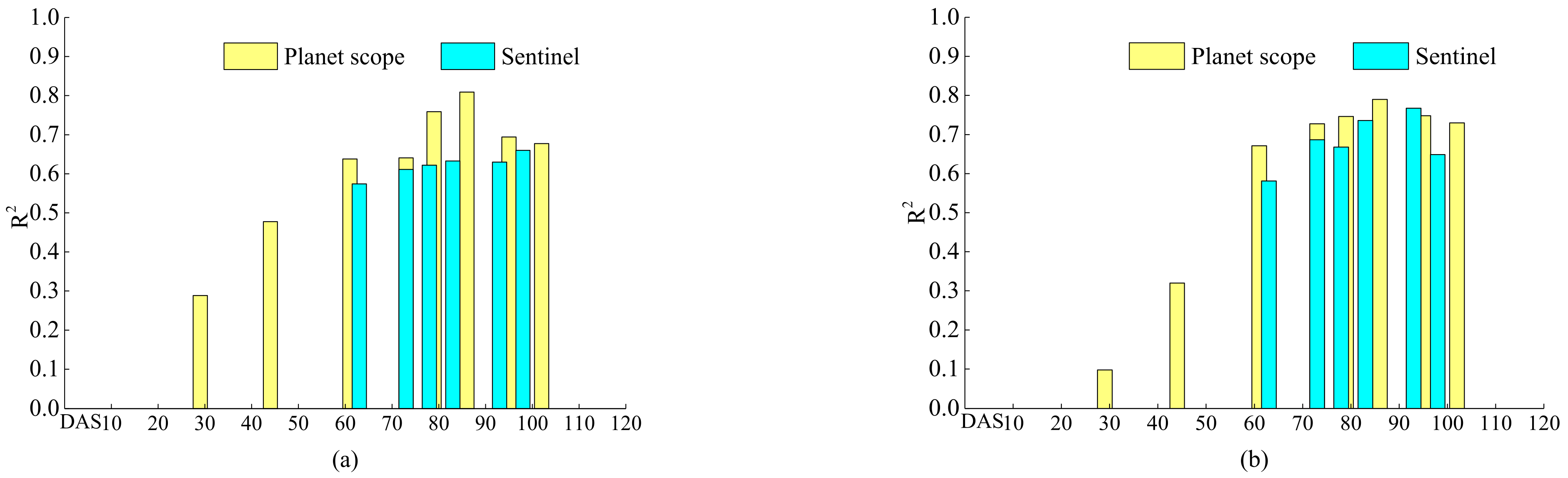
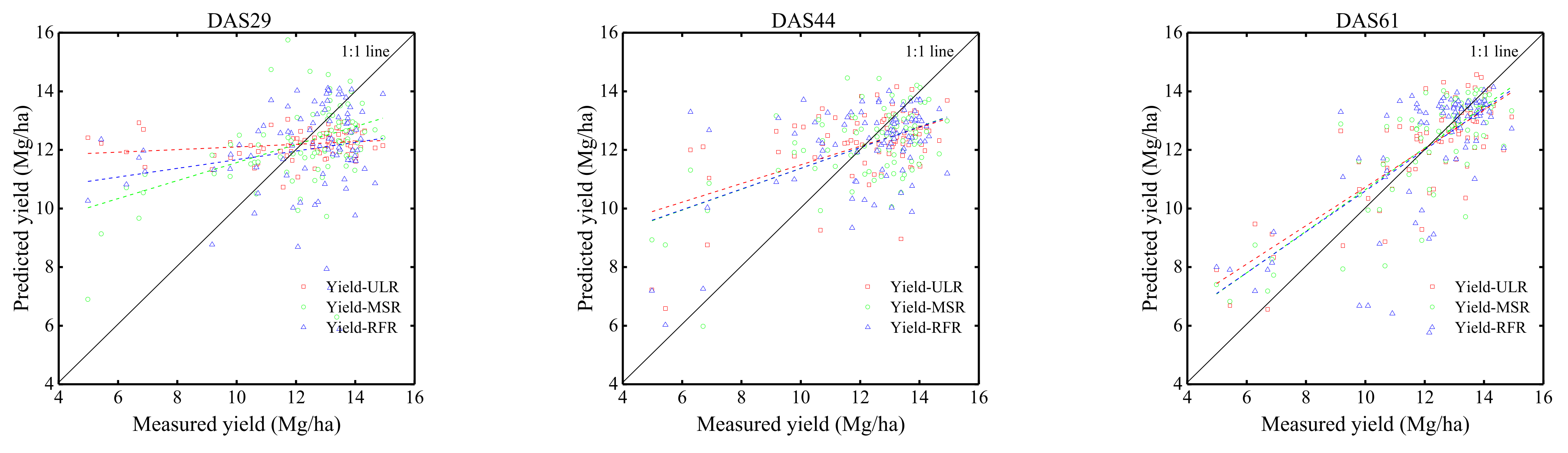
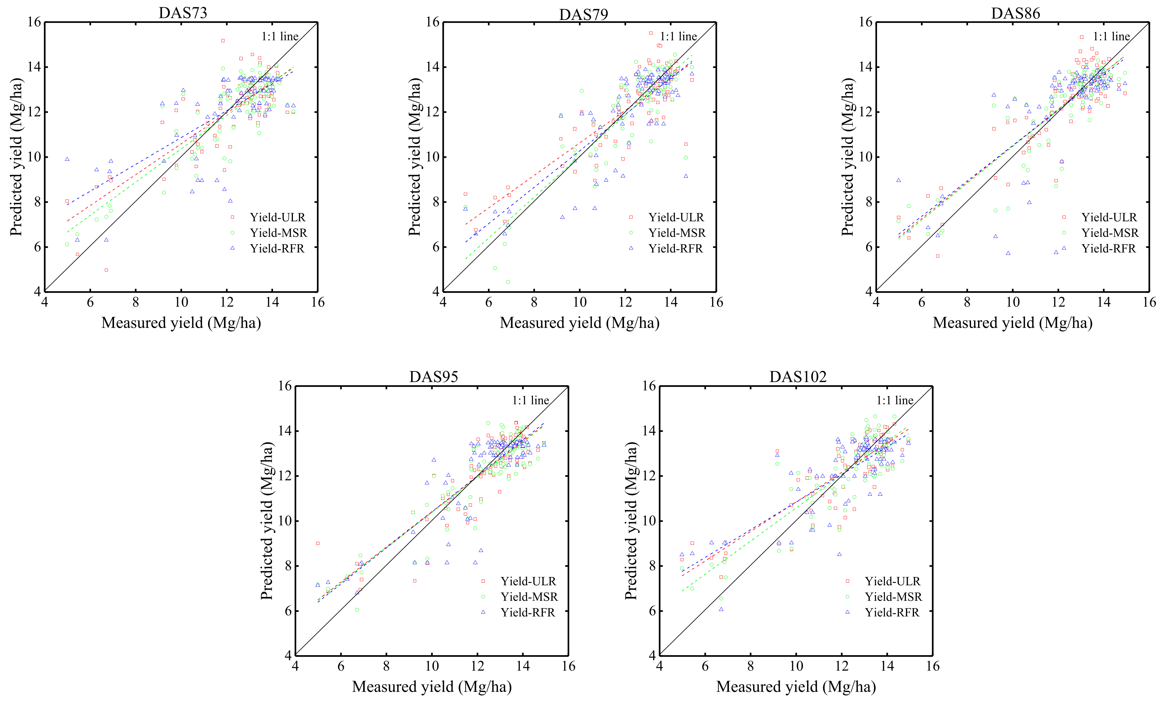
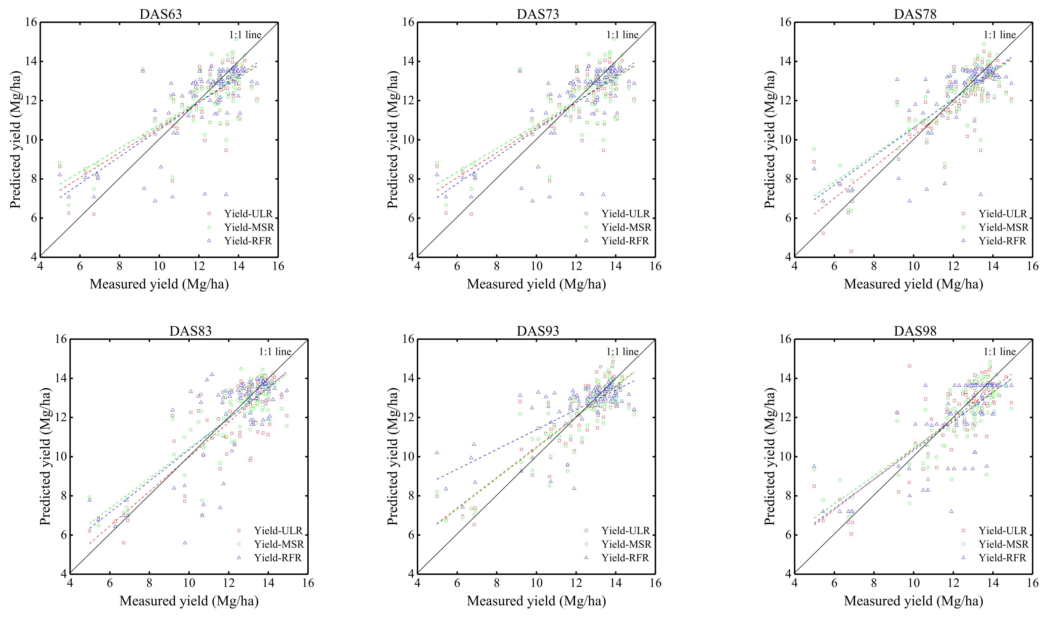
3.4.1. Yield-ULR Model

According to the correlation analysis results above, the Yield-ULR model at each growth stage was built based on the VI with the highest correlation as the independent variable. All VIs were linearly correlated with corn yield. The performance of each estimation model was summarized in

Table 3. The best Yield-ULR models constructed with PlanetScope and Sentinel-2 images.

Yield-ULR Model Based on PlanetScope Images				Yield-ULR Model Based on Sentinel-2 Images
Growth Stage	Models	R2	RMSE	Growth Stage	Models	R2	RMSE
DAS29	−11.06MCARI2 + 16.15	0.03	2.27
DAS44	34.68GNDVI − 9.40	0.32	1.91
DAS61	1.99GCVI − 4.99	0.61	1.45	DAS63	1.46GCVI + 1.10	0.56	1.53
DAS73	1.69GCVI − 5.44	0.60	1.46	DAS73	2.76GCVI − 1.28	0.48	1.65
DAS79	1.69GCVI − 493	0.64	1.38	DAS78	1.54GCVI − 1.03	0.58	1.49
DAS86	2.20GCVI − 6.78	0.72	1.22	DAS83	1.32GCVI + 0.31	0.57	1.51
DAS95	1.81GCVI − 3.85	0.65	1.37	DAS93	1.27GCVI + 1.64	0.61	1.45
DAS102	2.21GCVI − 4.71	0.64	1.39	DAS98	1.01GCVI + 3.06	0.64	1.39

. Almost all the best Yield-ULR models were obtained by the GCVI at each growth stage except for DAS29 (MCARI2) and DAS44 (GNDVI). Much lower correlations were found between the yield and VIs at the early growth stage before V10 (DAS29 and DAS44). At these stages, the plant was in the early vegetative period and its future growth could be largely uncertain due to various environmental stresses or different field management strategies, resulting in less accurate predictions of corn grain yield. Field topdressing was carried out after this growth period. The GCVI derived from PlanetScope images could explain 72% variability in corn yield on DAS86, which is also the best estimation accuracy for yield prediction across the 8 growth stages. while the best yield estimation model constructed with Sentinel images was on DAS98, which explained 63.9% of the corn yield variability. During such stages from R2 (blistering) to R3 (milking), corn is in its early reproductive period having almost maximum plant greenness and photosynthetic capacity, thus indicating the potential yield.

3.4.2. Yield-SMLR Model

The ten VIs were used to construct the Yield-SMLR models by SMLR according to the AIC and significance test. The model accuracy and other details are shown in

Table 4. The accuracy of the PlanetScope-based Yield-SMLR model in each growth period.

Growth Stage	Independent Variables	AIC	R2	RMSE
DAS29	GCVI, GNDVI, MCARI2, SAVI, SR, WDRVI	129.97	0.29	1.95
DAS44	MSAVI, NDVI, SAVI, SR, WDRVI	101.10	0.48	1.67
DAS61	EVI2, GCVI, GNDVI, MCARI2, NDVI	69.20	0.64	1.39
DAS73	EVI2, GCVI, GNDVI, MCARI2, SR, WDRVI	70.48	0.64	1.38
DAS79	EVI2, GCVI, GNDVI, NDVI, SR, WDRVI	35.79	0.76	1.13
DAS86	EVI2, GCVI, GNDVI, MCARI2, SR, WDRVI	15.51	0.81	1.01
DAS95	EVI2, GCVI, GNDVI, NDVI, SR, WDRVI	56.52	0.69	1.28
DAS102	EVI2, GCVI, GNDVI, MCARI2, SR, WDRVI	61.24	0.68	1.31

and

Table 5. The accuracy of Sentinel-based Yield-SMLR model in each growth period.

Growth Stage	Independent Variables	AIC	R2	RMSE
DAS63	MCARI2, MSR, SAVI, SR, WDRVI	83.33	0.57	1.51
DAS73	EVI2, GCVI, GNDVI, MCARI2, MSAVI, NDVI, SAVI, SR, WDRVI	83.36	0.61	1.44
DAS78	EVI2, MCARI2, NDVI, SAVI, WDRVI	73.00	0.62	1.43
DAS83	EVI2, GCVI, GNDVI, MCARI2, MSAVI, NDVI, SAVI, SR, WDRVI	78.20	0.63	1.40
DAS93	EVI2, GNDVI, MCARI2, MSR, SAVI, SR, WDRVI	75.13	0.63	1.41
DAS98	EVI2, MCARI2, MSAVI, MSR, SAVI, WDRVI	54.51	0.66	1.26

. Yield-SMLR models performed better than the Yield-ULR ones. The coefficient of determination values ranged from 0.29 (DAS29) to 0.81 (DAS86) with PlanetScope images, and 0.57 (DAS63) to 0.66 (DAS98) with Sentinel-2 images. In the early growth stage (DAS29 and DAS44) for PlanetScope iamges, the indices related to soil background removal (SAVI and MSAVI) had a greater impact on the yield model due to the lower coverage. In the reproductive growth stage, VIs sensitive to the chlorophyll concentration in a wide range of chlorophyll variations, such as GCVI, GNDVI, and WDRVI contributed more to the yield estimation. However, maybe due to the coarse resolution of Sentinel data, yield could be well interpreted by combining MCARI2 and WDARVI (responsive to leaf chlorophyll concentration) with the SAVI and SAVI (sensitive to ground reflectance). In general, the PlanetScope-based Yield-SMLR models had lower AIC value than that of the Sentinel-based ones in a similar growth period. All the coefficients of the best PlanetScope-based Yield-SMLR on DAS86 passed the significance test (p < 0.01) and could be expressed as, Yield = 7595.13 − 43,343.22 EVI2 − 53.88 GCVI + 29,035.99 GNDVI + 43,528.09 MCARI2 − 81.58 SR + 38,108.57 WDRVI.

3.4.3. Yield-RFR Model

The ten VIs were also adopted to construct corn yield estimation models based on the RFR algorithm.

Table 6. The Yield-RFR model constructed with PlanetScope and Sentinel images (Parameters represented the n-estimations, max-features, and depth in RFR).

Yield-RFR Model with PlanetScope Images				Yield-RFR Model with Sentinel Images
Growth Stage	Parameters	R2	RMSE	Growth Stage	Parameters	R2	RMSE
DAS29	10, 70%, 5	0.75	1.10
DAS44	10, 80%, 8	0.82	0.96
DAS61	7, 70%, 6	0.85	0.86	DAS63	9, 90%, 3	0.81	1.01
DAS73	3, 60%, 10	0.79	1.05	DAS73	5, 100%, 4	0.78	1.07
DAS79	5, 80%, 7	0.86	0.84	DAS78	7, 50%, 3	0.82	0.97
DAS86	9, 100%, 10	0.90	0.73	DAS83	5, 50%, 10	0.85	0.86
DAS95	3, 100%, 12	0.80	1.05	DAS93	9, 70%, 12	0.89	0.75
DAS102	3, 50%, 7	0.78	1.09	DAS98	7, 50%, 3	0.85	0.88

clearly showed that Yield-RFR models captured the variability in corn yield over the growing season well, compared with Yield-ULR and Yield-SMLR models. The R² was improved from 0.81 to 0.90 at DAS86 for PlanetScope-based Yield-RFR model and 0.63 to 0.89 at DAS93 for sentinel-based ones (Table 6).

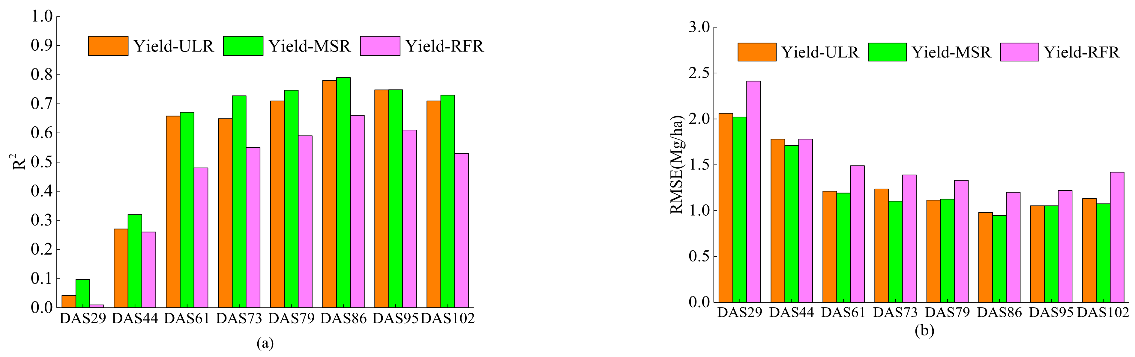
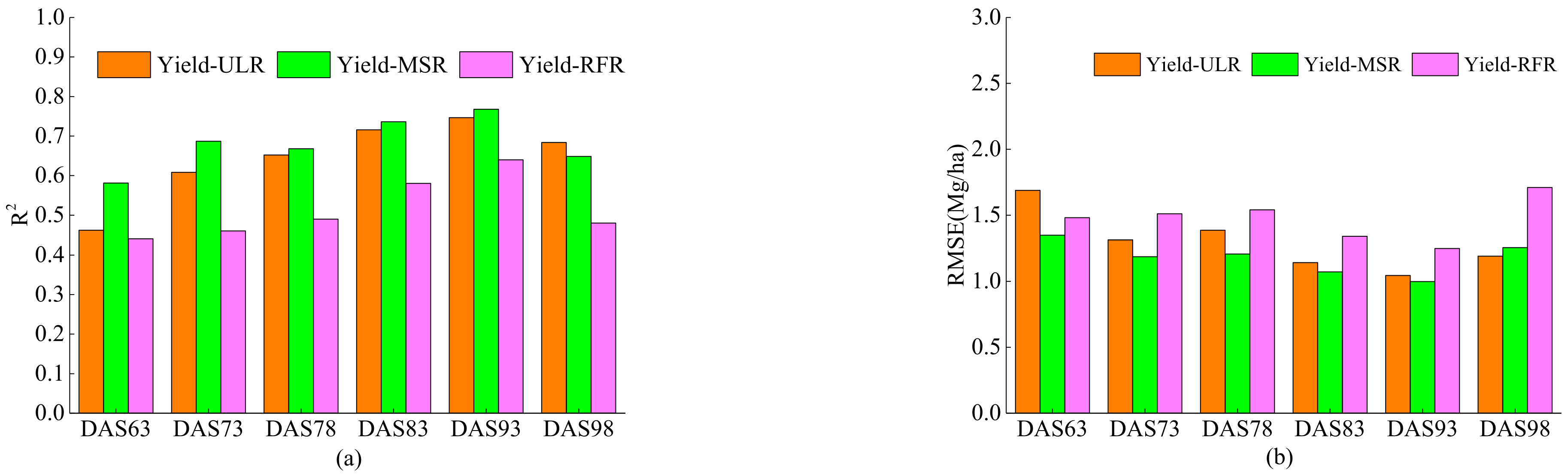
3.4.4. Model Comparison and Validation

The validation datasets were input into the optimal models above to assess the accuracy of each yield model. The performance of each model with PlanetScope images was summarized in Figure 3 based on R² and RMSE measurements. As shown in Figure 3, the performance of the RFR method was evidently lower than that of the ULR and SMLR approaches in each growth stage, which was contrary to the prediction results in Section 3.4.3 and may indicate overfitting problems in the ML modeling. Overall, among the three regression methods, the SMLR method performed the best, with the highest R² and lowest RMSE across the growing season. Significant increases in R² were observed across all yield prediction methods on DAS86, with the RMSE values of 0.98, 0.94, and 1.2 Mg·ha⁻¹ for Yield-ULR, Yield-SMLR, and Yield-RFR, respectively.

For the Sentinel-based models, similar results were presented (Figure 4). Figure 4 clearly showed that the SMLR method outperformed the ULR and RFR in corn yield prediction. The best prediction timing by the Yield-SMLR model was on DAS93, with the maximum correlation (R² = 0.77) and the minimum RMSE value of 0.99 Mg·ha⁻¹. This was followed by the DAS83, with the R² and RMSE values of 0.74 and 1.07 Mg·ha⁻¹, respectively.

Overall, results based on both satellite image sources showed that the best performing approach for corn yield estimation was SMLR. The highest R² and lowest RMSE values in validation sets were observed during the R2 to R3 stages (DAS86 for PlanetScope data and DAS93 for Sentinel data), which could explain 79% and 77% variability in corn yield. The optimal time to predict yield was later with Sentinel data than with PlanetScope data. Imagery was collected from both sensors on DAS73. The models could explain up to 73% of within-field yield variability with PlanetScope data, whereas, 68% with Sentinel-2 data. This was contributed to the different spatial resolutions. High spatial resolution imagery can more accurately reflect the crop growth status and capture the within-field variability of crop growth conditions (Figure 1b).

When comparing the corn yield prediction and validation results of both images together, it was observed that the Vis of PlanetScope images resulted in better performance in corn yield estimation than Sentinel images at similar growth stages both in the calibration and validation datasets (Figure 5). The prediction ability increased with the growth period before the vegetative growth stage, stabilized in the reproductive growth stage, and decreased slightly in the later stage after R3.

The scatter plots in Figure 6 and Figure 7 showed how well the predicted corn yields fitted the actual yields under different regression methods and growth stages. The predicted yield values were linearly correlated with the observed values (demonstrated by the dashed lines), while the correlation was less consistent in RFR. The larger deviations of the predicted corn yield from the 1:1 line indicated that all the estimation methods experienced higher levels of overestimation of corn yields at lower actual yields. The models gave the best estimation results when the corn yield was greater than 10 Mg·ha⁻¹, especially at the R2 and R3 growth stages.

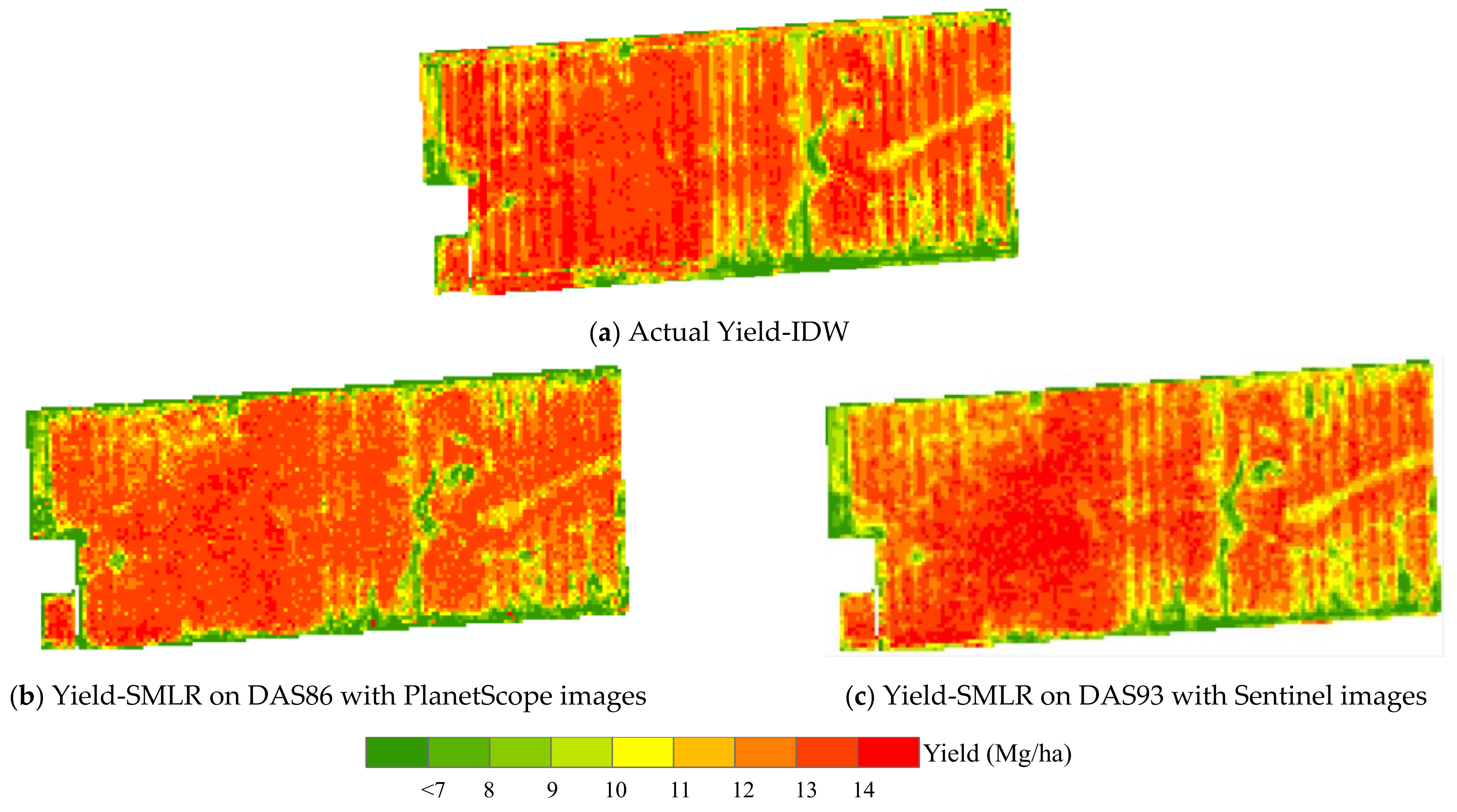
3.4.5. Corn Yield Mapping on Key Growth Stages with SMLR Method

Vegetation index matrices were substituted into the optimal Yield-SMLR models on DAS86 and DAS93 to map the corn yield. The field was symbolized by nine yield categories using an equal interval strategy based on the predicted grain yield (Figure 8). The prediction results were generally in good agreement with the actual distribution of corn yield. The loss of correlation might be due to different ground resolutions beween yield data (even after resampling) and actual satellite image ground resolution. Resampling from 3 m to 10 m of PlanetScope data caused a loss of spectral information, but it was still more informative than the 10 m sentinel data. The pattern observed confirmed that the resampled PlanetScope data outperformed Sentinel data for corn yield estimation. These results also highlighted the ability of the SMLR method to estimate corn grain yield before harvest at the field scale.

4. Discussion

4.1. Vegetation Index for Corn Yield Estimation

Spectral VIs provide composite properties of leaf chlorophyll, leaf area, optical measures of canopy greenness, and canopy structure, which lay a theoretical foundation for using VIs to estimate crop yield. RS methods for crop yield prediction currently rely on broadband VIs, such as the NDVI, EVI, SAVI, etc. [46]. Due to the different growth statuses and cultivars of crops, there were significant differences in VI selection and yield estimation accuracy [9]. Skakun et al. argued that the most important spectral bands explaining corn and soybean yield variability were green, RE, and NIR [33]. We computed 10 VIs from time-series of PlanetScope and Sentinel-2 data and analyzed the correlation between VIs and corn grain yield. It clearly showed that the GCVI captured the variability in corn yield well over the growing season except for DAS29 and DAS44, having the highest R² values in Yield-ULR models (Table 3), followed by GNDVI (Figure 2; Table 3). GCVI, GNDVI, EVI2, and WDRVI entered almost all Yield-SMLR models at each growth stage (Table 4). The variable importance measure of the RFR model illustrated the effects of each VI on the estimation of corn yield. We made statistics on the order of variable importance entering each RFR model (eight models with PlanetScope images and six from Sentinel images). Figure 9a showed the order statistics for each VI in all models. For example, GCVI appeared four times in the first importance (VIP1) of 14 models. Figure 9b showed the accumulated count for each importance. The variable importance statistics also confirmed the performance of GCVI and GNDVI, which appeared nine and six times, respectively, ranking in the top two positions in the variable importance lists for all models. Specific absorption coefficients of chlorophylls in the green spectral regions are much smaller than in the red region, which does not saturate at moderate to high chlorophyll contents. The GCVI and GNDVI were proposed by replacing the original red band with green band, which enabled more precise estimation of chlorophyll concentration in a greater dynamic range of chlorophyll variations, and were more sensitive to green crop LAI and biomass than the VIs calculated with red band, such as NDVI, SAVI, EVI2 and SR [33,52,58,61].

The results were consistent with reported studies. Based on Sentinel-2 images, Kayad et al. illustrated that GNDVI could provide the highest R² value of 0.48 for monitoring the within-field variability of corn grain yield [31]. Shanahan et al. compared NDVI, TSAVI, and GNDVI in estimating final grain yield for corn and indicated that GNDVI acquired during mid-grain filling was highly correlated with grain yield and could be used to produce relative yield maps depicting spatial variability in fields [28]. The Yield-ULR models showed a weak correlation with a single VI for evaluating grain yield, while Yield-SMLR and Yield-RFR models constructed through multiple VIs could enhance the prediction ability of corn yields. The Yield-SMLR model could explain 81% variability in corn yield on DAS86 with PlanetScope images, while Sentinel images could explain 66% variability on DAS98. In this study, since the within-field environmental variables such as topographical and meteorological conditions were relatively uniform and stable, the yield level could be indicated by crop growth status, which could be monitored by VIs sensitive to chlorophyll and biomass, especially the GCVI and GNDVI. In summary, this study demonstrated that it was feasible to monitor corn yields with VIs during a suitable growth period.

4.2. Model Selection for Corn Yield Estimation

VIs could be especially beneficial for corn yield estimation when used together. The RFR method did not achieve the expected accuracy perhaps due to the small dataset in this study [12,34]. Although RFR had a slightly higher R² and lower RMSE compared to other algorithms in the calibration models, better performance was achieved for corn yield using a SMLR method for the validation sets, which implied a better generalization capability of the SMLR than RFR and ULR. The RFR method incorporating various variables did not always show the highest estimation accuracy [28]. In Sakamoto’s study, the performance of the proposed RFR method was about the same or slightly worse, with a higher RMSE than the conventional polynomial regression model for corn grown in Iowa and Illinois [28]. This was probably because of an overfitting issue that caused accuracy deterioration against expectations [62]. In addition, at a regional scale, the cropland ecosystem was complex and many of the processes involved were nonlinear, which made the ML algorithm possible [63]. However, the analysis in this field-scale study revealed a linear correlation relationship between the VIs and corn yield, which may imply corn yield prediction within-field was not best represented in nonlinear models in this study. The SMLR method has been widely investigated to determine the best feature subsets for crop yield prediction [64] and had acceptable corn yields estimation capability in this study. This method selected more important VIs according to the AIC to build a yield estimation model. When a VI had an insignificant effect on the output, the model after removing this variable would still show high correlation and low RMSE. The superiority of the SMLR could be attributed to its ability to detect all possible combinations between input variables and gave the optimal subset of input variables.

4.3. Remote Sensing Data Selection for Yield Estimation

RS is an attractive tool for monitoring spatiotemporal patterns of vegetation growth, which enhances the process of monitoring the development of agricultural crops and estimating their yields. The relatively high yield estimation accuracy was obtained using high resolution satellite images. At present, Sentinel-2 imagery was considered the most suitable remotely sensed data for crop yield estimation at field level [11]. Al-Gaadi et al. [65] revealed that Sentinel-2 images enabled the reduction in the generalization in crop spectral reflection and delineation of sharp field boundaries so that the relationship between actual and predicted potato yield values produced an R² value that increased from 0.39 for Landsat-8 images to 0.47 for Sentinel-2 images. Hunt et al. [7] demonstrated that Sentinel-2 data was more accurate at 10 m resolution than 20 m for within-field wheat yield in the UK. When compared Landsat data with Sentinel-2 and PlanetScope, only 59% of yield variability could be explained with 30 m image data. They thought the rest was lost because of coarsening and mixture effects inside the 30 m pixel [33]. This study compared Planetcsope and Sentinel-2 satellite images for corn yield estimation, and the resampled PlanetScope data explained 15% more corn yield variability than the Sentinel-2 data at the same spatial resolution of 10 m (Table 4). Although PlanetScope images were resampled to the resolution of 10 m, they still had relatively detailed and accurate canopy information than the Sentinel data. This may imply that high spatial-resolution satellite data has the potential to provide relatively accurate estimates of yield variability at the field scale.

4.4. Timing for Corn Yield Estimation by Remotely Sensed Data

Identifying the best timing will be beneficial to farmers and crop management to accurately predict yield well ahead of harvest time with minimal remotely sensed data. The growth characteristics of corn in the vegetative growth stage may not fully reflect the accumulation of organic matter in yield organs at the late mature stage, resulting in poor prediction accuracy of corn grain yield. The tasseling stage is a critical transition period for corn from vegetative growth to reproductive growth. It is believed that the fastest matter accumulation and the most fertilizer absorption stage occur from 10 days before tasseling to 25 to 30 days after tasseling. The corn growth from the tasseling stage to silking stage directly determined the dry matter accumulation of crop yield organs.

Unganai and Kogan found that a corn yield estimation model could be constructed with VIs approximately 6 weeks prior to harvest time from the 1.1 km spatial-resolution AVHRR Data in southern Africa [45]. Results from MODIS data and county-level statistical yields revealed that the optimal time was typically in the late vegetative growing season, 13 days before the silking stage for corn in the USA [28]. The best time for wheat yield prediction with the 30 m spatial-resolution Landsat 8 was found to be the beginning of the full biomass period from the 138th to 167th day of the year [66]. Based on field measured corn yield, the precision of the Yield-SMLR model increased over time (Table 4) with sentinel-2 images in this study, reflecting that it was more accurate to predict corn yield near the harvest than in the earlier growth stages. This result was consistent with the findings by Kayad et al. [34]. Their study demonstrated that Sentinel-2 images could provide a clear description of the corn grain yield at the within-field scale during the physiological maturity stages (R4–R6), crop ages of 105 to 135 days from planting in North Italy. The results with PlanetScope images indicated that corn yield could be accurately estimated when high spatial-resolution satellite data was available during the crop growing period between the R2 (blistering) and R3 (milking) stages with prediction accuracy above 81%. It is not surprising that this stage could be used to estimate the corn yield. At the end of silking stage, the maximum plant height is achieved, and the potential kernel number is determined. After this stage, the nutrients in corn are transferred to grains in the maturity stage and the chlorophyll content in leaves decreases. Therefore, the correlation between the VI and crop yield decreases, which leads to a low yield estimation accuracy. Our results suggested that R2 (DAS86) was the most suitable phenological stage for corn yield estimation in this study area using PlanetScope images.

The digitization footprint estimation indicated that the total amount of field data accumulated by farmers increased to over 768 MB/ha in 2020 [67]. Among them, remotely sensed data from different platforms played a major contribution. In terms of digitization footprint contribution, the image data storage of 6.5 KB/ha (PlanetScope image on DAS86) would be used instead of 76.6 KB/ha (8 PlanetScope and 6 Sentinel 2A images) for corn yield estimation in this study. According to the best yield prediction model, the storage of VIs used for yield estimation at DAS86 is about 8.4 KB/ha. Yield prediction during the optimal growth period can greatly reduce the storage of remote sensing data.

4.5. Research Challenge

Although satellite RS data are very valuable due to their large-scale coverage, spatial resolution is still a concern in yield estimation at the field and within-field scales. This study demonstrated that it was possible to predict the corn grain yield at the field level with VIs based on PlanetScope images during R2 to R3 growth stage. Certainly, more studies are needed to further evaluate the SMLR and ML models using larger datasets. Years of yield data and more fields are needed to verify the estimation accuracy. In addition, averaging 6 m yield values to the 10 m resolution reduces the variance of yield that could be explained with satellite data, therefore increasing the coefficient of determination [33]. Further research is needed to explore the 6 m yield estimation ability with 3 m Planetscope data only.

5. Conclusions

Vegetation indices derived from PlanetScope and Sentinel-2 images were employed to investigate the potential of estimating corn yield with regression methods. Results from this study clearly showed that high spatial-resolution PlanetScope satellite imagery could be used to detect the corn yield variability at the field level, and it could explain 15% more variability than Sentinel-2 data at the same spatial resolution of 10 m. The green chlorophyll vegetation index (GCVI) values consistently produced the highest correlations with corn yield, accounting for 72% of the observed spatial variation in corn yield. More reliable quantitative yield estimation could be made using a SMLR method with multiple VIs. Good agreement between the observed and predicted yields was achieved with the coefficient of determination value being 0.81 at 86 days after seeding. More studies are needed to further evaluate the SMLR and ML models using larger datasets.

References

1. Medina, H.; Tian, D.; Abebe, A. On optimizing a MODIS-based framework for in-season corn yield forecast. Int. J. Appl. Earth Obs. 2021, 95, 102258. [Google Scholar] [CrossRef]
2. Tian, H.; Wang, P.; Tansey, K.; Han, D.; Zhang, J.; Zhang, S.; Li, H. A deep learning framework under attention mechanism for wheat yield estimation using remotely sensed indices in the Guanzhong Plain, PR China. Int. J. Appl. Earth Obs. 2021, 102, 102375. [Google Scholar] [CrossRef]
3. Zhao, Y.; Potgieter, A.B.; Zhang, M.; Wu, B.; Hammer, G.L. Predicting wheat yield at the field scale by combining high-resolution Sentinel-2 satellite imagery and crop modelling. Remote Sens. 2020, 12, 1024. [Google Scholar] [CrossRef] [Green Version]
4. Chahbi, A.; Zribi, M.; Lili-Chabaane, Z.; Duchemin, B.; Shabou, M.; Mougenot, B.; Boulet, G. Estimation of the dynamics and yields of cereals in a semi-arid area using remote sensing and the SAFY growth model. J. Remote Sens. 2014, 35, 1004–1028. [Google Scholar] [CrossRef] [Green Version]
5. Wu, S.; Yang, P.; Ren, J.; Chen, Z.; Li, H. Regional winter wheat yield estimation based on the WOFOST model and a novel VW-4DEnSRF assimilation algorithm. Remote Sens. Environ. 2021, 255, 112276. [Google Scholar] [CrossRef]
6. Dhakar, R.; Sehgal, V.K.; Chakraborty, D.; Sahoo, R.N.; Mukherjee, J.; Ines, A.V.M.; Shirasth, P.B.; Roy, S.B. Field scale spatial wheat yield forecasting system under limited field data availability by integrating crop simulation model with weather forecast and satellite remote sensing. Agric. Syst. 2022, 195, 103299. [Google Scholar] [CrossRef]
7. Hunt, M.L.; Blackburn, G.A.; Carrasco, L.; Redhead, J.W.; Rowland, C.S. High resolution wheat yield mapping using Sentinel-2. Remote Sens. Environ. 2019, 233, 111410. [Google Scholar] [CrossRef]
8. Johnson, D.M. An assessment of pre-and within-season remotely sensed variables for forecasting corn and soybean yields in the United States. Remote Sens. Environ. 2014, 141, 116–128. [Google Scholar] [CrossRef]
9. Liaqat, M.U.; Cheema, M.J.M.; Huang, W.; Mahmood, T.; Zaman, M.; Khan, M.M. Evaluation of MODIS and Landsat multiband vegetation indices used for wheat yield estimation in irrigated Indus Basin. Comput. Electron. Agric. 2017, 138, 39–47. [Google Scholar] [CrossRef]
10. Wang, J.; Dai, Q.; Shang, J.; Jin, X.; Sun, Q.; Zhou, G.; Dai, Q. Field-scale rice yield estimation using sentinel-1A synthetic aperture radar (SAR) data in coastal saline region of Jiangsu Province, China. Remote Sens. 2019, 11, 2274. [Google Scholar] [CrossRef]
11. Segarra, J.; González-Torralba, J.; Aranjuelo, Í.; Araus, J.L.; Kefauver, S.C. Estimating wheat grain yield using Sentinel-2 imagery and exploring topographic features and rainfall effects on wheat performance in Navarre, Spain. Remote Sens. 2020, 12, 2278. [Google Scholar] [CrossRef]
12. Azadbakht, M.; Ashourloo, D.; Aghighi, H.; Homayouni, S.; Shahrabi, H.S.; Matkan, A.; Radiom, S. Alfalfa yield estimation based on time series of Landsat 8 and PROBA-V images: An investigation of machine learning techniques and spectral-temporal features. Remote Sens. Appl. Soc. Environ. 2022, 25, 100657. [Google Scholar] [CrossRef]
13. Bendig, J.; Bolten, A.; Bennertz, S.; Broscheit, J.; Eichfuss, S.; Bareth, G. Estimating biomass of barley using crop surface models (CSMs) derived from UAV-based RGB imaging. Remote Sens. 2014, 6, 10395–10412. [Google Scholar] [CrossRef] [Green Version]
14. Johnson, M.D.; Hsieh, W.W.; Cannon, A.J.; Davidson, A.; Bédard, F. Crop yield forecasting on the Canadian Prairies by remotely sensed vegetation indices and machine learning methods. Agric. For. Meteorol. 2016, 218, 74–84. [Google Scholar] [CrossRef]
15. Zhang, M.; Zhou, J.; Sudduth, K.A.; Kitchen, N.R. Estimation of maize yield and effects of variable-rate nitrogen application using UAV-based RGB imagery. Biosyst. Eng. 2020, 189, 24–35. [Google Scholar] [CrossRef]
16. Yang, W.; Nigon, T.; Hao, Z.; Paiao, G.D.; Fernández, F.G.; Mulla, D.; Yand, C. Estimation of corn yield based on hyperspectral imagery and convolutional neural network. Comput. Electron. Agric. 2021, 184, 106092. [Google Scholar] [CrossRef]
17. Wan, L.; Cen, H.; Zhu, J.; Zhang, J.; Zhu, Y.; Sun, D.; Du, X.; Zhai, L.; Weng, H.; Li, Y.; et al. Grain yield prediction of rice using multi-temporal UAV-based RGB and multispectral images and model transfer–a case study of small farmlands in the South of China. Agric. For. Meteorol. 2020, 291, 108096. [Google Scholar] [CrossRef]
18. Franch, B.; Bautista, A.S.; Fita, D.; Rubio, C.; Tarrazó-Serrano, D.; Sánchez, A.; Skakun, S.; Vermote, E.; Becker-Reshef, I.; Uris, A. Within-Field Rice Yield Estimation Based on Sentinel-2 Satellite Data. Remote Sens. 2021, 13, 4095. [Google Scholar] [CrossRef]
19. Fortin, J.G.; Anctil, F.; Parent, L.É.; Bolinder, M.A. Site-specific early season potato yield forecast by neural network in Eastern Canada. Precis. Agric. 2011, 12, 905–923. [Google Scholar] [CrossRef]
20. Feng, A.; Zhou, J.; Vories, E.D.; Sudduth, K.A.; Zhang, M. Yield estimation in cotton using UAV-based multi-sensor imagery. Biosyst. Eng. 2020, 193, 101–114. [Google Scholar] [CrossRef]
21. Ashapure, A.; Jung, J.; Chang, A.; Oh, S.; Yeom, J.; Maeda, M.; Maeda, A.; Dube, N.; Landivar, J.; Hague, S.; et al. Developing a machine learning based cotton yield estimation framework using multi-temporal UAS data. ISPRS J. Photogramm. Remote Sens. 2020, 169, 180–194. [Google Scholar] [CrossRef]
22. Xu, W.; Chen, P.; Zhan, Y.; Chen, S.; Zhang, L.; Lan, Y. Cotton yield estimation model based on machine learning using time series UAV remote sensing data. Int. J. Appl. Earth Obs. 2021, 104, 102511. [Google Scholar] [CrossRef]
23. Gutiérrez, S.; Wendel, A.; Underwood, J. Ground based hyperspectral imaging for extensive mango yield estimation. Comput. Electron. Agric. 2019, 157, 126–135. [Google Scholar] [CrossRef]
24. Apolo-Apolo, O.E.; Martínez-Guanter, J.; Egea, G.; Raja, P.; Pérez-Ruiz, M. Deep learning techniques for estimation of the yield and size of citrus fruits using a UAV. Eur. J. Agron. 2020, 115, 126030. [Google Scholar] [CrossRef]
25. Sumesh, K.C.; Ninsawat, S.; Som-ard, J. Integration of RGB-based vegetation index, crop surface model and object-based image analysis approach for sugarcane yield estimation using unmanned aerial vehicle. Comput. Electron. Agric. 2021, 180, 105903. [Google Scholar]
26. Doraiswamy, P.C.; Hatfield, J.L.; Jackson, T.J.; Akhmedov, B.; Prueger, J.; Stern, A. Crop condition and yield simulations using Landsat and MODIS. Remote Sens. Environ. 2004, 92, 548–559. [Google Scholar] [CrossRef]
27. Guan, K.; Wu, J.; Kimball, J.S.; Anderson, M.C.; Frolking, S.; Li, B.; Hain, C.R.; Lobell, D.B. The shared and unique values of optical, fluorescence, thermal and microwave satellite data for estimating large-scale crop yields. Remote Sens. Environ. 2017, 199, 333–349. [Google Scholar] [CrossRef] [Green Version]
28. Sakamoto, T. Incorporating environmental variables into a MODIS-based crop yield estimation method for United States corn and soybeans through the use of a random forest regression algorithm. ISPRS J. Photogramm. Remote Sens. 2020, 160, 208–228. [Google Scholar] [CrossRef]
29. Siyal, A.A.; Dempewolf, J.; Becker-Reshef, I. Rice yield estimation using Landsat ETM + Data. J. Appl. Remote Sens. 2015, 9, 095986. [Google Scholar] [CrossRef]
30. Claverie, M.; Ju, J.; Masek, J.G.; Dungan, J.L.; Vermote, E.F.; Roger, J.C.; Skakun, S.V.; Justice, C. The Harmonized Landsat and Sentinel-2 surface reflectance data set. Remote Sens. Environ. 2018, 219, 145–161. [Google Scholar] [CrossRef]
31. Lambert, M.J.; Traoré, P.C.S.; Blaes, X.; Baret, P.; Defourny, P. Estimating smallholder crops production at village level from Sentinel-2 time series in Mali’s cotton belt. Remote Sens. Environ. 2018, 216, 647–657. [Google Scholar] [CrossRef]
32. Schwalbert, R.A.; Amado, T.J.C.; Nieto, L.; Varela, S.; Corassa, G.M.; Horbe, T.A.N.; Rice, C.W.; Peralta, N.R.; Ciampitti, I.A. Forecasting maize yield at field scale based on high-resolution satellite imagery. Biosyst. Eng. 2018, 171, 179–192. [Google Scholar] [CrossRef]
33. Skakun, S.; Kalecinski, N.I.; Brown, M.G.L.; Johnson, D.M.; Vermote, E.F.; Roger, J.; Franch, B. Assessing within-field corn and soybean yield variability from WorldView-3, Planet, Sentinel-2, and Landsat 8 satellite imagery. Remote Sens. 2021, 13, 872. [Google Scholar] [CrossRef]
34. Kayad, A.; Sozzi, M.; Gatto, S.; Marinello, F.; Pirotti, F. Monitoring within-field variability of corn yield using Sentinel-2 and machine learning techniques. Remote Sens. 2019, 11, 2873. [Google Scholar] [CrossRef] [Green Version]
35. Tomíček, J.; Mišurec, J.; Lukeš, P. Prototyping a Generic Algorithm for Crop Parameter Retrieval across the Season Using Radiative Transfer Model Inversion and Sentinel-2 Satellite Observations. Remote Sens. 2021, 13, 3659. [Google Scholar] [CrossRef]
36. Mudereri, B.T.; Dube, T.; Adel-Rahman, E.M.; Niassy, S.; Kimathi, E.; Landmann, T. A comparative analysis of PlanetScope and Sentinel-2 space-borne sensors in mapping Striga weed using Guided Regula rised Random Forest classification ensemble. Int. Arch. Photogramm. Remote Sens. Spat. Inf. Sci. 2019, 42, 701–708. [Google Scholar] [CrossRef] [Green Version]
37. Sadeh, Y.; Zhu, X.; Dunkerley, D.; Walker, J.P.; Zhang, Y.; Rozenstein, O.; Manivasagam, V.S.; Chenu, K. Fusion of Sentinel-2 and PlanetScope time-series data into daily 3 m surface reflectance and wheat LAI monitoring. Int. J. Appl. Earth Obs. 2021, 96, 102260. [Google Scholar] [CrossRef]
38. Pantazi, X.E.; Moshou, D.; Alexandridis, T.; Whetton, R.L.; Mouazen, A.M. Wheat yield prediction using machine learning and advanced sensing techniques. Comput. Electron. Agric. 2016, 121, 57–65. [Google Scholar] [CrossRef]
39. Gaso, D.V.; Berger, A.G.; Ciganda, V.S. Predicting wheat grain yield and spatial variability at field scale using a simple regression or a crop model in conjunction with Landsat images. Comput. Electron. Agric. 2019, 159, 75–83. [Google Scholar] [CrossRef]
40. Řezník, T.; Pavelka, T.; Herman, L.; Lukas, V.; Širucek, P.; Leitgeb, S.; Leitner, F. Prediction of yield productivity zones from Landsat 8 and Sentinel-2A/B and their evaluation using farm machinery measurements. Remote Sens. 2020, 12, 1917. [Google Scholar] [CrossRef]
41. Jaafar, H.H.; Ahmad, F.A. Crop yield prediction from remotely sensed vegetation indices and primary productivity in arid and semi-arid lands. J. Remote Sens. 2015, 36, 4570–4589. [Google Scholar] [CrossRef]
42. Battude, M.; Bitar, A.A.; Morin, D.M.; Cros, J.; Huc, M.; Sicre, C.M.; Dantec, V.L.; Demarez, V. Estimating maize biomass and yield over large areas using high spatial and temporal resolution Sentinel-2 like remote sensing data. Remote Sens. Environ. 2016, 184, 668–681. [Google Scholar] [CrossRef]
43. Shanahan, J.F.; Schepers, J.S.; Francis, D.D.; Varvel, G.E.; Wilhelm, W.W.; Tringe, J.M.; Schlemmer, M.R.; Major, D.J. Use of remote-sensing imagery to estimate corn grain yield. Agron. J. 2001, 93, 583–589. [Google Scholar] [CrossRef] [Green Version]
44. Panda, S.S.; Ames, D.P.; Panigrahi, S. Application of vegetation indices for agricultural crop yield prediction using neural network techniques. Remote Sens. 2010, 2, 673–696. [Google Scholar] [CrossRef] [Green Version]
45. Unganai, L.S.; Kogan, F.N. Drought monitoring and corn yield estimation in Southern Africa from AVHRR data. Remote Sens. Environ. 1998, 63, 219–232. [Google Scholar] [CrossRef]
46. Chlingaryan, A.; Sukkarieh, S.; Whelan, B. Machine learning approaches for crop yield prediction and nitrogen status estimation in precision agriculture: A review. Comput. Electron. Agric. 2018, 151, 61–69. [Google Scholar] [CrossRef]
47. Bierman, P.M.; Rosen, C.J.; Venterea, R.T.; Lamb, J.A. Survey of nitrogen fertilizer use on corn in Minnesota. Agric. Syst. 2012, 109, 43–52. [Google Scholar] [CrossRef]
48. Planet Team. Planet Imagery Product Specifications; Planet Labs Inc.: San Francisco, CA, USA, 2018; Available online: https://www.planet.com/products/satellite-imagery/files/Planet_Combined_Imagery_Product_Specs_December2017.pdf (accessed on 12 April 2018).
49. Jordan, C.F. Derivation of leaf-area index from quality of light on the forest floor. Ecology 1969, 50, 663–666. [Google Scholar] [CrossRef]
50. Chen, J.M. Evaluation of vegetation indices and a modified simple ratio for boreal applications. Can. J. Remote Sens. 1996, 22, 229–242. [Google Scholar] [CrossRef]
51. Rouse, J.W.; Hass, R.H.; Schell, J.A.; Deering, D.W. Monitoring vegetation systems in the great plains with ERTS. Third Earth Resour. Technol. Satell. Symp. 1973, 1, 309–317. [Google Scholar]
52. Gitelson, A.A.; Kaufman, Y.J.; Merzlyak, M.N. Use of a green channel in remote sensing of global vegetation from EOS-MODIS. Remote Sens. Environ. 1996, 58, 289–298. [Google Scholar] [CrossRef]
53. Baret, F.; Jacquemoud, S.; Hanocq, J.F. The soil line concept in remote sensing. Remote Sens. Rev. 1993, 7, 65–82. [Google Scholar] [CrossRef]
54. Jiang, Z.; Huete, A.R.; Didan, K.; Miura, T. Development of a two-band enhanced vegetation index without a blue band. Remote Sens. Environ. 2008, 112, 3833–3845. [Google Scholar] [CrossRef]
55. Haboudane, D.; Miller, J.R.; Pattey, E.; Zarco-Tejada, P.J.; Strachan, I.B. Hyperspectral vegetation indices and novel algorithms for predicting green LAI of crop canopies: Modeling and validation in the context of precision agriculture. Remote Sens. Environ. 2004, 90, 337–352. [Google Scholar] [CrossRef]
56. Qi, J.; Chehbouni, A.; Huete, A.R.; Kerr, Y.H.; Sorooshian, S. A modified soil adjusted vegetation index. Remote Sens. Environ. 1994, 48, 119–126. [Google Scholar] [CrossRef]
57. Gitelson, A.A. Wide dynamic range vegetation index for remote quantification of biophysical characteristics of vegetation. J. Plant Physiol. 2004, 161, 165–173. [Google Scholar] [CrossRef] [Green Version]
58. Gitelson, A.A.; Viña, A.; Arkebauer, T.J.; Rundquist, D.C.; Keydan, G.; Leavitt, B. Remote estimation of leaf area index and green leaf biomass in maize canopies. Geophys. Res. Lett. 2003, 30, 1248. [Google Scholar] [CrossRef] [Green Version]
59. R Core Team. R: A Language and Environment for Statistical Computing. R Foundation for Statistical Computing, Vienna, Austria. 2017. Available online: https://www.R-project.org (accessed on 12 April 2018).
60. Breiman, L. Random forests. Mach. Learn. 2001, 45, 5–32. [Google Scholar] [CrossRef] [Green Version]
61. Lobell, D.B.; Thau, D.; Seifert, C.; Engle, E.; Little, B. A scalable satellite-based crop yield mapper. Remote Sens. Environ. 2015, 164, 324–333. [Google Scholar] [CrossRef]
62. Belgiu, M.; Drăguţ, L. Random forest in remote sensing: A review of applications and future directions. ISPRS J. Photogramm. Remote Sens. 2016, 114, 24–31. [Google Scholar] [CrossRef]
63. Mkhabela, M.S.; Bullock, P.; Raj, S.; Wang, S.; Yang, Y. Crop yield forecasting on the Canadian Prairies using MODIS NDVI data. Agric. For Meteorol. 2011, 151, 385–393. [Google Scholar] [CrossRef]
64. Gopal, P.M.; Bhargavi, R. Performance evaluation of best feature subsets for crop yield prediction using machine learning algorithms. Appl. Artif. Intell. 2019, 33, 621–642. [Google Scholar]
65. Al-Gaadi, K.A.; Hassaballa, A.A.; Tola, E.K.; Kayad, A.G.; Madugundu, R.; Alblewi, B.; Assiri, F. Prediction of potato crop yield using precision agriculture techniques. PLoS ONE 2016, 11, e0162219. [Google Scholar] [CrossRef] [PubMed]
66. Nagy, A.; Szabó, A.; Adeniyi, O.D.; Tamás, J. Wheat Yield Forecasting for the Tisza River Catchment Using Landsat 8 NDVI and SAVI Time Series and Reported Crop Statistics. Agronomy 2021, 11, 652. [Google Scholar] [CrossRef]
67. Kayad, A.; Sozzi, M.; Paraforos, D.S.; Rodrigues, F.A., Jr.; Cohen, Y.; Fountas, S.; Francisco, M.; Pezzuolo, A.; Grigolato, S.; Marinello, F. How many gigabytes per hectare are available in the digital agriculture era? A digitization footprint estimation. Comput. Electron. Agric. 2022, 198, 107080. [Google Scholar] [CrossRef]
Figure 1. Location of the study area. (a) Study area and sample dataset distribution; (b) True color composite red-green-blue of PlanetScope (left) and Sentinel-2 A (right) images on 17 July 2018.
Agronomy 12 03176 g001
Figure 2. Coefficient of determination (R²) between VIs and corn yield at different growth stages based on (a) PlanetScope images and (b) Sentinel-2 images.
Agronomy 12 03176 g002
Figure 3. Model validation in each growth stage based on PlanetScope images. (a) R2 and (b) RMSE.
Agronomy 12 03176 g003
Figure 4. Model validation in each growth stage based on Sentinel images. (a) R2 and (b) RMSE.
Agronomy 12 03176 g004
Figure 5. R2 difference between PlanetScope images and Sentinel images based on SMLR method. (a) Calibration set and (b) Validation set.
Agronomy 12 03176 g005
Figure 6. Scatter plots of the measured versus predicted corn yields with different regression methods in each growth stage based on PlanetScope images. (Dashed red line, green line, blue line and black solid line are the regression line of Yield-ULR, Yield-SMLR and Yield-RFR, and1:1 line, respectively).
Agronomy 12 03176 g006aAgronomy 12 03176 g006b
Figure 7. Scatter plots of the measured versus predicted corn yields with different regression methods in each growth stage based on Sentinel images. (Dashed red line, green line, blue line and black solid line are the regression line of Yield-ULR, Yield-SMLR and Yield-RFR, and1:1 line, respectively).
Agronomy 12 03176 g007
Figure 8. Maps of simulated grain yield by the proposed regression models.
Agronomy 12 03176 g008
Figure 9. Variable importance for modelling corn yield with random forest regression. (a) The order statistics for each VI in all RFR models (eight models with PlanetScope images and six from Sentinel images). (b) The statistics of accumulated count for VIs in all RFR models.
Agronomy 12 03176 g009