LiDAR Odometry and Mapping Based on Semantic Information for Maize Field

Abstract

Agricultural environment mapping is the premise of the autonomous navigation of agricultural robots. Due to the undulating terrain and chaotic environment, it is challenging to accurately map the environmental maize field using existing LOAM (LiDAR odometry and mapping) methods. This paper proposes a LOAM method based on maize stalk semantic features for 6-DOF (degrees of freedom) pose estimation and field mapping with agricultural robots operating in a dynamic environment. The piecewise plane fitting method filters the ground points for the complex farmland terrain. To eliminate the unstable factors in the environment, we introduce the semantic information of maize plants into the feature extraction. The regional growth method segments the maize stalk instances, the instances are parameterized to a line model, and the optimization method calculates the pose transformation. Finally, the mapping method corrects the drift error of the odometry and outputs the maize field map. This paper compares our method with the GICP and LOAM methods. The trajectory relative errors of our method are 0.88%, 0.96%, and 2.12%, respectively, better than other methods. At the same time, the map drawn by our method has less ghosting and clearer plant edges. The results show that our method is more robust and accurate than other methods due to the introduction of semantic information in the environment. The mapping of corn fields can be further used in precision agriculture.

1. Introduction

With the increasing cost of agricultural labor, accelerating agricultural modernization and developing smart agriculture has become the development direction of China’s agriculture [1,2,3]. The intelligent agricultural robot is a critical component of intelligent agriculture [4,5,6]. Deploying intelligent robots is appealing for a variety of applications, including yield and health estimating [7,8], as well as weed detection [9], pest detection [10], and disease detection [11]. Among the capabilities of an intelligent robot, map building and state estimation are among the most fundamental prerequisites. The map can estimate yield and health, calculate planting density, row spacing, and plant spacing in the plot unit, and measure plant height and growth detection in the unit of a single plant.

To realize the long-term autonomous navigation of agricultural robots with more accuracy and lower cost, based on the simultaneous localization and mapping (SLAM) technology, the LiDAR (Light Detection And Ranging) sensor is used to draw the map of the environment while detecting the crop plants.

Mapping has been applied to orchards [12,13], forests [14], and agricultural scenes. Underwood et al. [15] used the hidden semi-Markov model to segment individual trees, introduced a descriptor to represent the appearance of each tree, and then associated new observations with the map of the orchard. Guo et al. [16] used the target ball to reconstruct a single fruit tree. In large-scale agricultural scene reconstruction, Su et al. [17] and Qiu et al. [18] used tools such as target ball to construct salient features for point cloud registration. Manuel et al. [19,20] obtained the positioning information of acquisition tools for point cloud registration. Dong et al. [21] and Sun et al. [22] extracted features from images for scene reconstruction.

Before the SLAM method, the most commonly used method in two-frame LiDAR scanning wasICP (Iteration closest point) [23] and NDT (Normal distribution transformation) [24]. Many variants of ICP methods have been proposed to improve efficiency and accuracy, including point-to-plane ICP [25], GICP (Generalized-ICP) [26], and point-to-line ICP [27]. However, when the number of points is more, the computational cost of the ICP method is more. In addition, the ICP method has low robustness in the dynamic environment.

Therefore, feature-based matching methods have attracted more attention as they require fewer computational resources by extracting representative features from the environment. Many feature detectors have been proposed [28,29], such as FPFH (Fast Point Feature Histogram) [30]. Serafin et al. [31] proposed a method to extract plane and line features from sparse point clouds quickly and verified the accuracy of the feature extraction method combined with the SLAM method.

Because the feature extraction method is simple and effective, more and more SLAM methods use feature extraction to build LiDAR odometry. Ji et al. [32] classified the points into plane points and edge points by calculating the smoothness and then matching the plane points and edge points with the plane and line segments of the next frame to calculate the transformation. This method obtains the highest accuracy of the LiDAR odometer in the KITTI dataset. Shan et al. [33] proposed the LeGO-LOAM method to improve the LOAM method, the points in the environment were segmented, the plane points and edge points were detected according to the smoothness, and the matching of segmented labels was added based on the LOAM matching method. Jiang et al. [34] divided the points into voxels, calculated the geometric features of the voxel, matched the features with the feature labels according to the distance, and integrated the Partition of Unity (POU)-based feature extraction method into the SLAM system. The SegMatch [35] method first segmented the point cloud, then extracted its eigenvalues and shape histograms, and used a random forest classifier to match the segmentation in the two scans. Chen et al. [36] proposed a LiDAR odometer and mapping framework used in forestry environments. Firstly, the ground and trunk examples were segmented, and the plane and cylindrical parameters were extracted as features for data association. This method has certain universality.

The above methods have achieved high accuracy in public datasets or specific application scenarios, but they are not suitable for the farmland environment. In the maize planting environment, adjacent maize usually has a similar appearance, making it difficult to distinguish similar plants. On the other hand, due to the influence of wind, maize is very easy to deform, which leads to inconsistency in the appearance of the same maize plant even in the data of two adjacent frames. Therefore, in the intensive planting environment, the above LOAM method cannot extract representative features and perform accurate feature matching when the maize changes dynamically.

Our work focuses on solving the LOAM problem of the autonomous system working in the maize field. Previous methods rely on texture features and are fragile in the farmland environment. Therefore, this paper presents a semantic-based LOAM method. The key idea is to extract robust maize stalk features using semantic information and extract maize stalk instances as parameterized landmarks to obtain a robust LOAM solution.

The method includes (1) ground filtering with a piecewise plane fitting method; (2) maize stalk detection with a regional growth method; (3) landmark model parameter extraction; (4) data association and motion estimation; and (5) LiDAR mapping. The primary contributions of this paper are as follows:

• A maize stalk detection pipeline is developed, and maize stalk instance is parameterized into a landmark model.
• A LOAM method can perform robust data association, and ego-motion estimation in maize intensive planting environments is developed.
• Our method is verified by maize field data of different growth states.

2. Materials and Methods

2.1. Hardware and Sensors

The 3D point cloud data used in this study were obtained through the mobile robot platform controlled by the joystick that navigated in the experimental field. The LiDAR scanner used in this study is an RS-LiDAR-32 (Robosense, Shenzhen, China) mounted at the height of 1.2 m. The installation angle of LiDAR can be adjusted in the range of 0°~−15°. The specifications of the LiDAR can be found in

Table 1. Key parameters of RS-LiDAR-32.

Key Parameters	Values
LiDAR class	32 laser lines
Field of view/scanning angle	360 degrees
Vertical field of view	40 degrees
Azimuth angular resolution	0.1 degrees
Vertical angular resolution	0.33 degrees
Accuracy	<3 cm distance accuracy
Operation range (distance)	0.4 m to 200 m range

. In order to compensate for the influence of rough terrain and mechanical vibration on the LiDAR, the robot platform is equipped with an Inertial Measurement Unit (IMU). GNSS receiver is mounted on a mobile robot platform to obtain ground truth. The mobile robot platform and its composition are shown in Figure 1.

2.2. Software System Overview

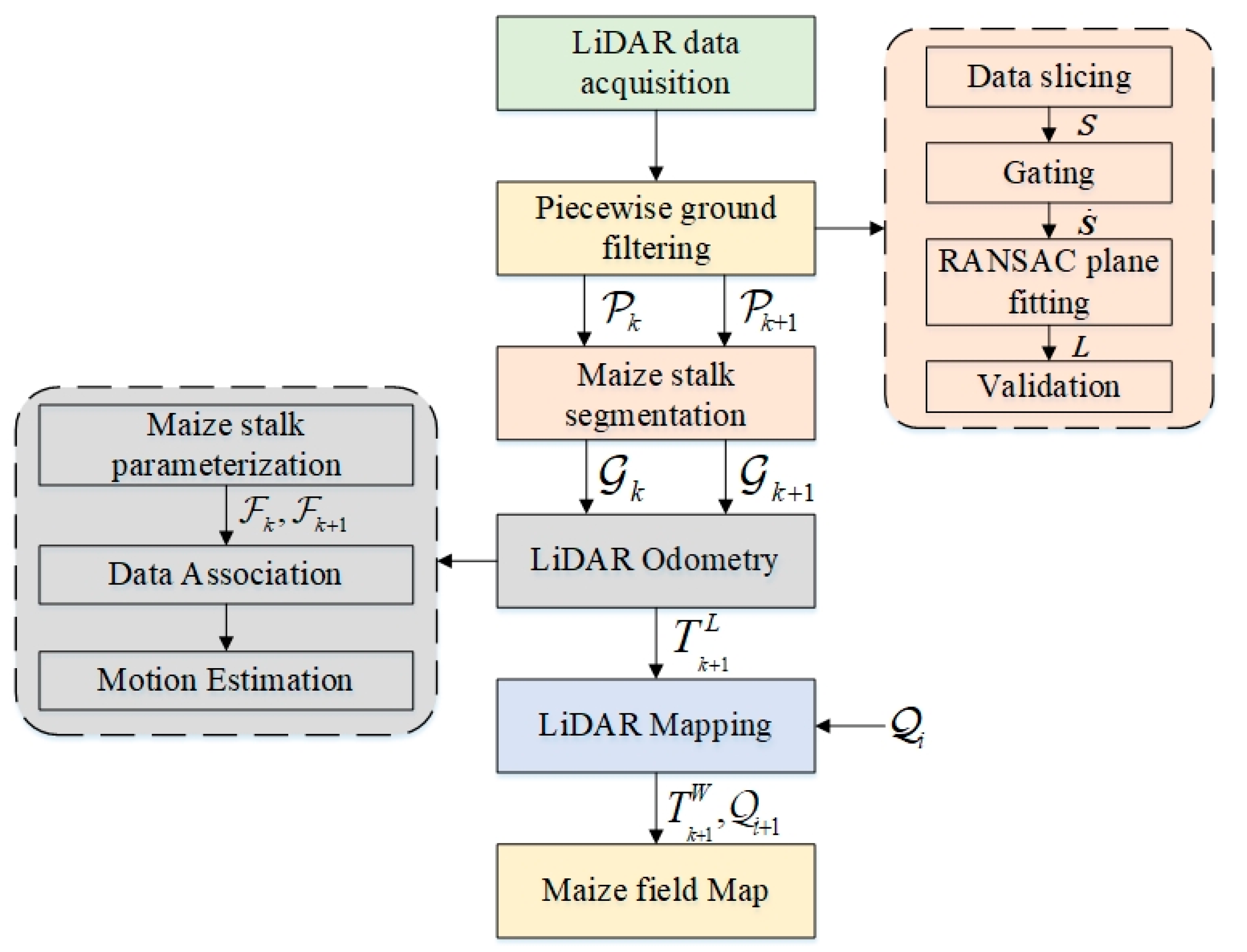
Figure 2 shows the data processing flow chart of our LiDAR odometry and mapping method. Because the LOAM method has better real-time and scalability, our method adopts a framework similar to the LOAM method.

The problem is to perform an ego-motion estimation with a point cloud perceived by LiDAR in a maize field and build a map for the agricultural environment. A sweep refers to the point cloud obtained by LiDAR completing one scan coverage.${\mathcal{P}}_k$ indicates the point cloud perceived during a sweep k. Firstly, the ground points are filtered by the piecewise ground filtering method for the current sweep ${\mathcal{P}}_{k+1}$ and the previous sweep ${\mathcal{P}}_k$, the maize stalk instances are detected by the maize stalk segmentation method. Take ${\mathcal{P}}_k$ as an example, maize stalk instances with a number of $N_k$ are put into set ${\mathcal{G}}_k\triangleq {\left\{{\mathcal{G}}_k^i\right\}}_{i=1}^{N_k}$. At the same time, feature points with a number of $N_j$ contained in a stalk instance is put into set ${\mathcal{G}}_k^i\triangleq {\left\{p_j\right\}}_{j=1}^{N_j}$. Next, for each ${\mathcal{G}}_k^i$, the landmark parameters are extracted into ${\mathcal{F}}_k\triangleq {\left\{f_k^i\right\}}_{i=1}^{N_k}$, and the number of landmark parameters is the same as the number of stalk instances. Finally, the pose transforms $T_{k+1}^L$ are estimated by data association and motion estimation, where $T_{k+1}^L$ is the LiDAR pose transform between points in LiDAR coordinate {L}.

The LiDAR mapping algorithm is executed to process the odometry output further and calculate the $T_{i+1}^W$. $T_{i+1}^W$ refers to the LiDAR pose transform in world coordinate {W}. Finally, the map ${\mathcal{Q}}_i$ is updated to ${\mathcal{Q}}_{i+1}$.

2.3. Piecewise Ground Filtering

Many methods assume that the ground is flat and everything that stands up from the ground is considered an obstacle. However, the ground is not always planar in the actual agricultural scenes encountered by autonomous robots. Nonplanar grounds, such as undulated and sloped terrains, curved uphill/downhill ground surfaces, or situations with big rolling/pitch angles of the autonomous robots remain unsolved. We modified the method of Asvadi et al. [37] to make it suitable for agricultural ground filtering. This method can automatically and accurately fit the ground without manual modification of parameters. The method includes four steps: (1) data slicing; (2) gating; (3) RANSAC plane fitting; (4) validation.

2.3.1. Data Slicing

This process divides point cloud data into different slices with the mobile robot platform position as the origin. Firstly, the Pass-Through filter removes the points outside the region of interest (ROI). The axis range of the ROI was set to 0~10 m, and the axis range was set to −5~5 m. The LiDAR scanning harness model is established, as shown in Figure 3.

Since there is a certain range of blind areas around the acquisition platform, the radius is related to the installation angle. According to the geometric relationship, the distance from the front end of the initial slice to the center of the mobile robot platform $R_0$ is:

$$R_0=h·arctan\left(\frac{\pi }{2}-{\alpha }_L-{\alpha }_b\right)$$

(1)

The angle between the front end of the initial area and the vertical line of the LiDAR installation position ${\alpha }_0=\arctan \left(R_0/\mathrm{h}\right)$. Then the distance from the front end of each slice to the mobile robot platform $R_i$ is:

$$R_i=h·tan\left({\alpha }_0+i·\eta ·\Delta \alpha -{\alpha }_L\right)$$

(2)

where h is the height of the LiDAR sensor to the ground;${\alpha }_L$ is the LiDAR mount angel;${\alpha }_b$ is the minimum vertical angle of the LiDAR laser transmitter; $\eta$ is the number of scanning harnesses for LiDAR data in each region; $\Delta \mathsf{\alpha }$ is the vertical resolution of LiDAR, (°). Considering$\mathcal{P}={\left\{p_j=\left(x_j,y_j,z_j\right)\right\}}_{j=1}^{N_p}$ of size $N_p$, each region is represented as $S={\left\{s_i:R_{i-1}<p_j<R_i\right\}}_{i=1}^N$ of size N.

2.3.2. Gating

$\mathcal{P}$ includes plant points and ground points. Because the height (z-value) and distribution are very different, plant points belong to the abnormal point in the plane fitting. Selecting ground data as much as possible can improve the accuracy of the plane fitting. The IQR (interquartile range) method automatically selects the z-value range. The IQR is:

$$IQR=Q_3-Q_1$$

(3)

where $Q_1$ is the first quartile of z-value; $Q_3$ is the third quartile of z-value. Then the upper and lower gate limits of the z-value can be calculated as follows:

$$\left\{\begin{array}{c}{Q}_{\min }=Q_1-0.5\times IQR\\ Q_{\max }=Q_3-0.5\times IQR\end{array}\right.$$

(4)

The ground filtering accuracy is the highest when the IQR coefficient is 0.5 after many tests. After obtaining the upper and lower gate limits of the z-value, the points within the gate are selected for surface plane fitting. The point within the gate in each region $s_i$ is represented as $\dot{s_i}$. The gating operation is shown in Figure 4.

2.3.3. RANSAC Plane Fitting

The RANSAC (Random Sample Consensus) method is used to fit the ground plane to the inliers points. The RANSAC method is a random parameter estimation method that estimates the best model parameters from a group of observation data iteratively containing outliers. For the ground point in the kth slice $\dot{s_i}$, the RANSAC method randomly selects three points in $\dot{s_k}$ to fit the plane model.

The distance is calculated from each point to the plane. When the distance is below a given threshold, the point is chosen as an inliers point. The score is calculated as the number of inliers points. The plane that has the largest number of inliers is chosen as the best fit for the ground point. The fitting plane model is defined as ${\alpha }_{i}x+b_{i}y+c_{i}z+d_i=0$, denoted by $L={\left\{l_i=\left(a_i,b_i,c_i,d_i\right)\right\}}_{i=1}^N$.

2.3.4. Validation

Based on the assumption that the nearest slice $s_1$ has the maximum confidence of the fitting plane, the plane parameters are verified from the nearest slice to the farthest slice. For the two planes $G_{i-1}$ and $G_i$, calculate the angle ${\delta }_{{\psi }_i}$ between the normal and the distance ${\delta }_{z_i}$ between two planes. Let the angle threshold ${\psi }_{threshold}$= 15° and the distance threshold $Z_{threshold}$ = 0.05 m. When ${\delta }_{{\psi }_i}$ and ${\delta }_{z_i}$ meet the requirements, the plane $G_i$ is assumed valid. Otherwise, the parameters of $G_{i-1}$ are passed to $G_i$.

After the above steps are performed, the ground surface points are filtered according to the parameters of each slice. The specific method calculates the distance from each point to the plane, presets the distance threshold, and filters out all points whose distance is less than the threshold and points below the plane.

The ground filtering effects of different growth stages are shown in Figure 5. The first row is the plane detected by each region and the ground points, in which different planes and points are represented by different colors, respectively, and the second row is the segmented plant points and ground points, which are represented by two colors, respectively. It can be seen intuitively that our method filters out the uneven farmland surface point cloud, and the accuracy is quantitatively analyzed in Section 3.1.

2.4. Maize Stalk Segmentation

According to the comparison of the elastic modulus of the maize stalk and maize leaf, the maize stalk is less likely to deform under the influence of wind force than the maize leaf. Therefore, the primary purpose of this section is to divide each maize stalk point in the maize field. The overall workflow of the segmentation method is shown in Figure 6.

The regional growth method is used to segment the maize stalk point cloud. First, the initial seed points are detected by slicing. According to the L, the slice with a thickness of 0.05 m is extracted at z = 0.27 m above the plane (This value can be changed according to the height of the maize plant). Then the DBSCAN (Density-Based Spatial Clustering of Applications with Noise) method is applied to cluster the point cloud data in the slice. The DBSCAN method has two important parameters. Neighborhood radius$R_{eps}$, is used to calculate the density of a point and adjacent points, and the minimum preset number of points $R_{MinPts}$, in a single point neighborhood is used to classify each point into a class of core points, boundary points, and noise points. In this paper, $R_{eps}$ and $R_{MinPts}$ are set to 0.1 and 5. In maize planting, the fixed row spacing can generally be guaranteed. Therefore, the clustering results are further verified by fitting the planting line to exclude the clustering results of non-stem points, so the seed point set, ${\mathcal{P}}_{seed}$, is obtained. An example of a seed point extraction method is shown in Figure 7.

Second, two methods are adopted for regional growth and the selection of the next seed point. The choice of the two methods depends on the balance between computational efficiency and segmentation accuracy. In the first method, the slice with a size of 0.10 m × 0.10 m × 0.05 m is extracted below the current seed point, the DBSCAN clusters the data in the slice. The mean value of the clustering center is taken as the next seed point. The regional growth algorithm stops when the seed point cannot be found or reaches the lowest limit. The first method is simple and effective can quickly segment the stalk point cloud.

The second method adopts the method of paper by Jin et al. [38]. Extract the points $D={\left\{p_d:\Vert p_d-p_s{\Vert }_2\le R_d\right\}}_{d=1}^{N_d}$ of size N_d in the spherical area with radius $R_d$= 0.05 m around the seed point $P_s$, the growth direction m can be calculated by median normalized vector method:

$$\mathrm{m}=\mathrm{median}\left\{\frac{\left(p_d-p_s\right)}{\Vert p_d-p_s{\Vert }_2},p_d\subset D\right\}$$

(5)

where $\mathrm{median}\left\{\mathcal{·}\right\}$ stands for the median normalized value of the unit vector; $\Vert ·{\Vert }_2$ stands for L2 distance. The next seed point can be calculated as follows:

$$p_s^{\text{'}}=p_s+R_d\times \mathrm{m}$$

(6)

The regional growth algorithm stops when the seed point cannot be found or reaches the lowest limit. In the second method, the growth direction is determined by the distribution of the nearest neighbor points of the seed points. The second method can obtain more accurate segmentation results but requires more computing resources. The two different growth methods are shown in Figure 8.

Finally, through the regional growth method, all stalk points in the point cloud data are segmented, and the feature points of the segmented stem instance are put into, where N_j is the number of feature points.

2.5. LiDAR Odometry

2.5.1. Maize Stalk Parameterization

For each stalk instance in $G_k^i={\left\{p_j\right\}}_{j=1}^{N_j}$, the stalk is approximated as a straight line, and the line parameters are extracted as the characteristic parameters of each stalk instance. Let $f=\left(p_m,\mathrm{v}\right)$ be the parameters of a line model, where $p_m=\left(x_m,y_m,z_m\right)$ is a point on the line and $\mathrm{v}=\left(m,n,k\right)$ is the direction vector of the line. Considering that there may be some maize leaf points in $p_j$, the line parameter f in the feature points is still solved by the RANSAC method, and the line parameter f of each instance is put into $\mathcal{F}={\left\{f^i\right\}}_{i=1}^{N_k}$, where $N_k$ is the number of stalk instances.

2.5.2. Data Association and Motion Estimation

We need to find the corresponding stalk instance in the previous sweep for a stalk feature point $p_{k+1}^j\in {\mathcal{G}}_{k+1}^i$. We sequentially calculate the distance from each feature point $p_{k+1}^i$ to the line parameter $f_k^i$. The instances ${\mathcal{G}}_{k+1}^i$ corresponding to the line parameter $f_k^i$ are closest to most of the feature points in the set and can be regarded as the same instance. We perform data association by matching $G_{k+1}^i$ to the instance ${\overline{\mathcal{G}}}_k^j$ corresponding to the closest line parameter to most of the feature points in the set. In order to reduce false matching, we set the threshold of distance. The two instances do not perform data association when the distance exceeds the threshold. It is regarded as a suspected new landmark for an instance that has never been successfully matched with other instances. If it matches other instances successfully in the subsequent sweep, it will be used as a new landmark.

We can estimate the pose transform $T_{k+1}^L$ by optimizing the nonlinear least squares problem for the associated feature points and line parameters in two sweeps. The distance from a point to a line is selected as the error function. According to Huang et al. [39], compared with the point-to-point metric, a point-to-line metric gives quadratic convergence instead of linear convergence. It is proved that the point-to-line method can obtain higher accuracy in noisy data. Therefore, the error function is:

$$f\left(T_{k+1}^L\right)=argmin\frac{1}{2}{{\displaystyle \sum }}_{i=1}^{N_k}{\displaystyle \sum }_{j=1}^{N_i}{\left(\mathrm{v}\cdot \left(\mathrm{R}\times p_j+\mathrm{t}-p_m\right)\right)}^2$$

(7)

where $T_{k+1}^L=\left[\mathrm{t},\mathrm{R}\right]$ is the LiDAR pose transform between points ${\mathcal{P}}_k$,${\mathcal{P}}_{k+1}$ in LiDAR coordinate {L}. The nonlinear least squares problem (7) is solved by L-M (Levenberg–Marquardt) optimization.

Algorithm 1 shows the pseudo-code of our LiDAR odometry. The input of the algorithm is the mapped ${\overline{\mathcal{P}}}_k$, ${\overline{\mathcal{G}}}_k$, ${\overline{\mathcal{F}}}_k$, and current sweep ${\mathcal{P}}_{k+1}$. We run the piecewise ground surface filtering in ${\mathcal{P}}_{k+1}$, and the point cloud obtained is recorded as ${\tilde{\mathcal{P}}}_{k+1}$. Find the seed point set ${\mathcal{P}}_{seed}$ in ${\tilde{\mathcal{P}}}_{k+1}$, and obtain the feature point set ${\mathcal{G}}_{k+1}$ through region growing algorithm. Extract stem feature ${\mathcal{F}}_k$ from ${\mathcal{G}}_{k+1}$. Finally, the attitude transformation $T_{k+1}^L$ is obtained by solving Equation (7). Finally, according to the pose transform $T_{k+1}^L$, ${\mathcal{G}}_{k+1}$, ${\mathcal{F}}_{k+1}$, ${\mathcal{P}}_{k+1}$ are mapped to ${\overline{\mathcal{G}}}_{k+1}$, ${\overline{\mathcal{F}}}_{k+1}$, ${\overline{\mathcal{P}}}_{k+1}$ respectively. The algorithm outputs ${\overline{\mathcal{G}}}_{k+1}$, ${\overline{\mathcal{F}}}_{k+1}$, $T_{k+1}^L$. The algorithm cycles until the acquisition is completed.

Algorithm 1 LiDAR Odometry algorithm

1: Input: ${\overline{\mathcal{P}}}_k$, ${\overline{\mathcal{G}}}_k$, ${\overline{\mathcal{F}}}_k$, and ${\mathcal{P}}_{k+1}$ 2: Output: ${\overline{\mathcal{G}}}_{k+1}$,${\overline{\mathcal{F}}}_{k+1}$, and newly pose transform $T_{k+1}^L$ 3: for each point $p_j$ in ${\mathcal{P}}_{k+1}$ do 4:  Filtering the ground surface point by piecewise ground surface filtering to 5:   obtain ${\tilde{\mathcal{P}}}_{k+1}$ 6:  Find the seed point ${\mathcal{P}}_{seed}$ by slicing, DBSCAN clustering, and planting line fitting 7:  for each point in ${\mathcal{P}}_{seed}$ do 8:    Find feature point ${\mathcal{G}}_{k+1}$ by regional growth method 9:    for each point $p_{k+1}^j$ in ${\mathcal{G}}_{k+1}^i$ do 10:     Find $f_k^i$ by extracting stem parameters 11: end for 12: for each ${\mathcal{G}}_{k+1}$ and ${\mathcal{F}}_k$ do 13:  Update $T_{k+1}^L$ by solving (7) 14: end for 15: for ${\mathcal{G}}_{k+1}$, ${\mathcal{F}}_{k+1}$, and ${\mathcal{P}}_{k+1}$ do 16:  Project ${\mathcal{G}}_{k+1}$, ${\mathcal{F}}_{k+1}$, and ${\mathcal{P}}_{k+1}$ to${\overline{\mathcal{G}}}_{k+1}$, ${\overline{\mathcal{F}}}_{k+1}$, and ${\overline{\mathcal{P}}}_{k+1}$ 17: end for 18: return${\overline{\mathcal{G}}}_{k+1}$,${\overline{\mathcal{F}}}_{k+1}$, ${\overline{\mathcal{P}}}_{k+1}$,$T_{k+1}^L$

2.6. LiDAR Mapping

LiDAR odometry has obtained the pose transformation matrix of the LiDAR, but the map construction directly through the odometry output will produce inevitable cumulative errors. Therefore, the LiDAR odometry output is further optimized using the LiDAR mapping algorithm, and the newly obtained point cloud is mapped to the global map. The mapping algorithm is executed every 4 times of LiDAR odometry.

The mapping algorithm has similar input and output to the LiDAR odometry. The difference is that the LiDAR odometry calculates the pose transformation $T_{k+1}^L$ of the sensor in the vehicle coordinate system {L}, and the map building algorithm calculates the pose transformation $T_{i+1}^W$ of the sensor in the global coordinate system {W}.

The point cloud map is represented as $Q_i$, and the local point cloud map constructed from the output of LiDAR odometry 4 times is represented as $Q_{i+1}$. According to the pose transformation $T_{k+1}^L$ and the previous global pose transformation $T_i^W$, the same feature extraction as the laser odometry is implemented and finally obtains $T_{i+1}^W$ through the L-M algorithm.

3. Results

At the Shangzhuang experimental station of China Agricultural University (Beijing), the data of maize fields with growth days of 20 days, 48 days, 60 days, and 95 days were collected using the mobile robot platform. These data were used to verify the accuracy of the ground surface filtering and LiDAR odometry methods proposed in this paper. In the process of each data acquisition, different paths were selected according to the passable conditions. In each collection, the mobile robot platform traveled at a speed of 0.5 m/s in the maize field. The ground in each maize field was not flat, and the installation angle of LiDAR was adjusted according to the maize height during collection. The details of each experiment are listed in

Table 2. The details of each point cloud data.

Experiment	The Average Height of Maize/m	Average Scan Points	Trajectory Length/m
20 days	0.40	35,634	-
48 days	0.73	32,570	34.44
60 days	0.82	32,764	14.83
95 days	2.12	27,504	53.10

.

3.1. Ground Filtering Experiment

Ten frames of point cloud data collected at 20 days, 48 days, and 60 days were selected, respectively, with 30 frames. The point cloud data were manually divided into maize and ground surface points as ground truth. The ground filtering method based on piecewise plane fitting proposed in this paper is compared with the RANSAC method, the RANSAC method using the IQR method, and the LS method using the IQR method. For the method of manually setting parameters, the parameters with the highest accuracy and recall are used. The precision, recall, and average precision of the ground surface filtering method are calculated as follows:

$$R=\frac{TP}{TP+FN}$$

(8)

$$P=\frac{TP}{TP+FP}$$

(9)

$$AP=\frac{TP+TN}{TP+FP+TN+FN}$$

(10)

where R denotes the recall; P denotes the precision; AP denotes the average precision; TP is the true positives, which are the ground points commonly found in the reference and extracted ground points; FP is the false positives, which are the extracted ground points that are not present in the reference ground points; TN is the true negatives, which are the maize points commonly found in the reference and extracted maize points; and FN is the false negatives, which are the maize points that are not present in the reference ground points.

Table 3. Comparison of evaluation indexes of different ground surface filtering methods.

Experiment	Ours			RANSAC			IQR + RANSAC			IQR + LS
	P/%	R/%	AP/%	P/%	R/%	AP/%	P/%	R/%	AP/%	P/%	R/%	AP/%
20 days	94.32	88.17	86.49	81.61	80.39	66.64	89.23	86.35	80.62	80.41	72.13	65.73
48 days	92.27	88.29	85.13	78.35	83.44	66.57	86.19	91.96	84.45	79.84	73.85	68.42
60 days	91.34	87.34	85.71	74.26	80.24	63.28	84.64	87.90	83.17	65.51	68.93	58.40

shows the P, R, and AP of the ground surface filtering method. This phenomenon may be because with the increase in maize plant height, the shielding generated by plants will reduce the number of surface point clouds, resulting in the reduction in plane parameter calculation accuracy.

According to Table 3, the ground surface filtering method based on piecewise plane fitting achieves the highest P, R, and AP in maize point clouds of different growth days, in which the P is 94.32%, 92.27%, and 91.34%, respectively, the R is 88.17%, 88.29%, and 87.34%, respectively, and the AP is 86.49%, 85.13%, and 85.71%, respectively. In addition to our method, in this paper, the best method is the RANSAC method using the IQR method. It can be found from the table that the P, R, and AP of the method of setting parameters by the IQR method are higher than those of the method of manually setting parameters.

3.2. LiDAR Odometry and Mapping Method Experiment

We benchmarked our method with the LOAM and ICP methods. A-LOAM is an open-source implementation of the LOAM algorithm [32], and GICP is an open-source implementation of the ICP algorithm [26]. Both LOAM and ICP are commonly used. The LOAM method extracts line segment and plane features. Real-time mapping can be carried out through fast feature extraction and feature matching. High accuracy has been obtained in indoor and outdoor environment experiments. The ICP method has the highest accuracy in the case of small attitude transformation due to point-by-point registration, but it can not build maps in real time due to a large amount of calculation.

The data from the maize field collected at 48 days, 60 days, and 95 days were used as the method input. Then we evaluated the accumulated point cloud by evaluating whether each maize plant has ghosting and duplication. Quantitatively, we calculated the drift of motion estimation in each experiment, and counted the number of feature point sets in each sweep participating in registration and the number of correctly registered feature point sets.

It can be seen from Figure 9 that the maps generated by LOAM have ghosting. Although the map generated by GICP has no ghosting, the edge of each plant is not clear enough. This is due to the deformation of maize affected by wind, which leads to the calculation error of pose transfer. Our method only calculates the pose transfer of stalk point clouds with minor or no deformation to obtain the best point cloud map.

It can be seen from Figure 10 that the trajectory calculated by our method and the GICP method is the closest to the ground truth, the A-LOAM method deviates greatly from the ground truth, and the relative error is relatively large when handling large rotations. According to

Table 4. Distance and relative error of trajectory.

Experiment	Distance	Distance from the Goal/m			Error
		Ours	GICP	LOAM	Ours	GICP	LOAM
48 days	34.44	0.30	0.35	1.06	0.88%	1.01%	3.08%
60 days	14.83	0.14	0.17	0.67	0.96%	1.13%	4.52%
95 days	53.10	1.13	1.82	2.93	2.12%	3.43%	5.52%

, the accuracy of each LiDAR odometry decreases with the increase in maize growth days, which may be due to two reasons. On the one hand, the higher the maize plant is, the more serious the occlusion between plants is, and the fewer effective stalk instances can be extracted, which affects the accuracy of the LOAM method. On the other hand, most of the data obtained are maize leaf data, and the leaves are more affected by the wind. In particular, when the leaves are connected with adjacent maize stalks, the accuracy of segmentation and data association decreases significantly.

Compared with LOAM and GICP, our maize stalk feature is robust in dynamically transformed maize plants. Compared with the LOAM method, which extracts features based on line and plane, our method adds the semantic information of the environment, which makes the data association process more robust. Compared with the GICP method, our method ignores dynamically changing points and selects the stalk points that are not easy to transform in the dynamic environment, to reduce the pose transformation calculation error. Therefore, our method obtained the best accuracy of the three methods.

Table 5. The number of features matched successfully per sweep for different growth days.

Experiment	Number of Successfully Matched Features	Association Success Rates
48 days	23.2	89%
60 days	25.2	94%
95 days	15.1	95%

shows that for maize with different growth days, 23.2, 25.2, and 15.1 stalk instances with successful association can be extracted per sweep. The association success rate is calculated as the percentage between the correctly associated instances and all associated instances. The association success rates of each instance were 89%, 94%, and 95%, respectively. It indicates that the maize stalk feature extraction and matching method proposed in this paper can work with high precision.

Based on the above experiences, our SLAM method based on maize stalk feature points and parameter extraction can obtain high-precision pose transform results in maize fields with different growth days. The map obtained by our method can be used for single plant segmentation and maize growth parameter detection.

4. Discussion

This paper proposed a LOAM pipeline based on maize stalk instance segmentation for the maize field. Firstly, the uneven ground points are filtered by piecewise surface filtering. Secondly, the stem instance is segmented by a regional growth method. Thirdly, the pose transform is calculated by model parameter extraction, data association, and motion estimation. Finally, the LiDAR odometry output is accurately processed by a further LiDAR mapping method. Due to the introduction of stalk semantic information into LiDAR odometry and mapping, our method can accurately and robustly locate and map in outdoor maize intensive planting environments.

Comparing the other two LiDAR state estimation methods showed that our method can perform with high precision in a maize intensive planting environment. The relative errors of our method in maize field data of different growth states are 0.88%, 0.96%, and 2.12%, respectively. Our algorithm is more accurate with the maize with fewer growth days. Our algorithm can accurately extract the stem instance when the maize is relatively short. When the maize plant is high, the point of the maize stalk is far less than that of the maize leaf, and the leaf completely blocks the stalk. However, our algorithm achieves the highest accuracy compared with other methods. This is because we introduced the semantic information of maize stalks in the LOAM method, making our method robust to feature extraction and feature matching in the muddy maize fields, thus obtaining the highest accuracy.

It is essential for robots to locate themselves in an intensive maize planting environment. The map obtained by our method has no ghosting and blur and has the highest quality compared with other methods.

Although our method can deal with the deformation of maize, it does not solve the deformation of maize plants in the process of mapping. For example, suppose a leaf of a maize plant is displaced in two sweeps, our method can obtain accurate pose transformation. In that case, the ghosting of the same leaf will be generated in the mapping process, which leads to the decline in the quality of the map drawn by our method.

Finally, fusing multi-sensor data to obtain more accurate positioning information, further optimizing the execution speed of the algorithm, and applying the deep learning method to segment the stalk instance will be the focus of our future research.